1

4. DISCRETE PROBABILITY DISTRIBUTION

4.1 Useful series

(i) 1 2

1

nr

n

r

a a a a

=

= + + +∑ �

(ii) ( )1

11

2

n

r

r n n

=

= +∑

(iii) ( )( )2

1

11 2 1

6

n

r

r n n n

=

= + +∑

(iv) ( )0

nnr n r

r

nx y x y

r

−

=

= +

∑

(v) 1

0

1

1

nnr

r

xx

x

+

=

−=

−∑

(vi) 0

1 1

1

r

r

x xx

∞

=

= <−

∑

(vii) ( )0

11

nr

r

n rx x

r

∞−

=

+ − = −

∑

(viii) 0

rx

r

xe

r

∞

=

=∑

(ix) lim 1

nx

n

xe

n→∞

+ →

(x) 2

21

1

6r r

π∞

=

=

∑

(xi) ( )0

1n

nr

r

nx x

r=

= +

∑

(xii) 1

1

1 0

1

nnr

r

aa a

a

−

=

−= >

−∑

(xiii) ( )1

1

1 0 1

1

r

r

a aa

∞−

=

= < <−

∑

2

4.2 Uniform Distribution

Toss a die. The probability distribution of X , the number on the die, is given

below and illustrated by the vertical line graph.

x 1 2 3 4 5 6

( )P X x= 1/6 1/6 1/6 1/6 1/6 1/6

( )1

6P X x= = for 1,2,3,4,5,6x =

Definition: A random variable X has the a discrete uniform distribution if

and only if the probability distribution is given by

( ) ( )1

1,2,...,

0 otherwise

x kp x P X x k

=

= = =

Conditions for uniform model

� The discrete random variable X is defined over the set of ndistinct values

1 2, , , nx x x�

� Each value is equally likely to occur

1 2 3 4 5 6

0.10

0.12

0.14

0.16

0.18

0.20

0.22

x

P(X

=x)

3

Notation

(i) ( )~X Unif n

(ii) ( )1

2

nE X

+=

(iii) ( )2

1

2

nVar X

−=

(iv) Cdf: ( )

0

1

1

X

k a

k aF x a k b

n

k b

<

− + = ≤ ≤

>

where x denotes the greatest integer part of x .

Proof

We need to prove that the sum of ( )p x over its range equals 1.

So,

1 1

1 1 11 1

n n

x x

nn n n= =

= = × =∑ ∑

Proof (ii)

( ) ( )1

n

x

E X x P X x=

= =∑

1

1

n

x

xn =

= ∑

( )1

1 2 3 nn

= + + + +�

( )1 1

12 2

n nn

n

+ ⇒ + =

Proof (iii)

( ) ( )2 2Var X E X µ= −

( ) ( )2 2

1

n

x

E X x P X x=

= =∑

4

4.3 Bernoulli Distribution

Suppose you perform an experiment with two possible outcomes; either success

or failure. Success happens with probability p , while failure with probability 1 p−

A random variable that takes value 1 in case of success and 0 in case of failure is

called a Bernoulli random variable.

Definition: A random variable X has a Bernoulli distribution with parameter

p , if its probability mass function is:

( ) 1

1 0X

p xp x

p x

==

− =

or ( ) ( )1

1 0,1xx

Xp x p p x−

= − =

Notation

(i) ( )~X B p

(ii) ( )E X p=

(iii) ( ) ( )1Var X p p= −

(iv) Cdf: ( )

0 1

1 0 1

1 1

X

x

F x p x

x

<

= − ≤ < ≥

Proof

We need to prove that the sum of ( )p x over its range equals 1.

So: ( ) ( )1

0

1 1x

p x p p=

= − + =∑

5

Proof (ii)

( ) ( ) x

E X x P X x= =∑

( ) ( )1 1 0 0X Xp p= ⋅ + ⋅

( ) ( )1 0 1p p p⇒ + − =

Proof (iii)

( ) ( )2 2

x

E X x P X x= =∑

( ) ( )2 21 1 0 0X Xp p= ⋅ + ⋅

( ) ( )1 0 1p p p⇒ + − =

( )2 2E X p=

So: ( ) ( ) ( )2 2Var X E X E X= −

( )21p p p p⇒ − = −

6

4.4 Binomial Distribution

A binomial experiment is one that has the following properties:

a) the experiment consists of n identical trials which is fixed

b) the outcome of each trial is deemed either a success or a failure

c) the trials are independent

d) the probability, p of a successful outcome is the same for each trial. (The

probability of a failure, is 1q p= − )

� We are interested in x , the number of successes observed during the n trials

If the above four conditions are satisfied, then the random variable, X is said to

follow a binomial distribution.

Notation

(i) The distribution has two parameters ' 'n and ' 'p .

( )~ ,X Bin n p where n - number of trials and p - probability of success

(ii) ( ) n x n xxP X x C p q

−= = for 0,1,2,.....,x n=

(iii) ( )E X np=

(iv) ( )Var X npq=

Proof

We need to prove that the sum of ( )p x over its range equals 1.

( ) ( )0 0

1n n

n xx

x x

np x p p

x

−

= =

= −

∑ ∑

( ){ }1n

p p= + −

1 1n⇒ =

7

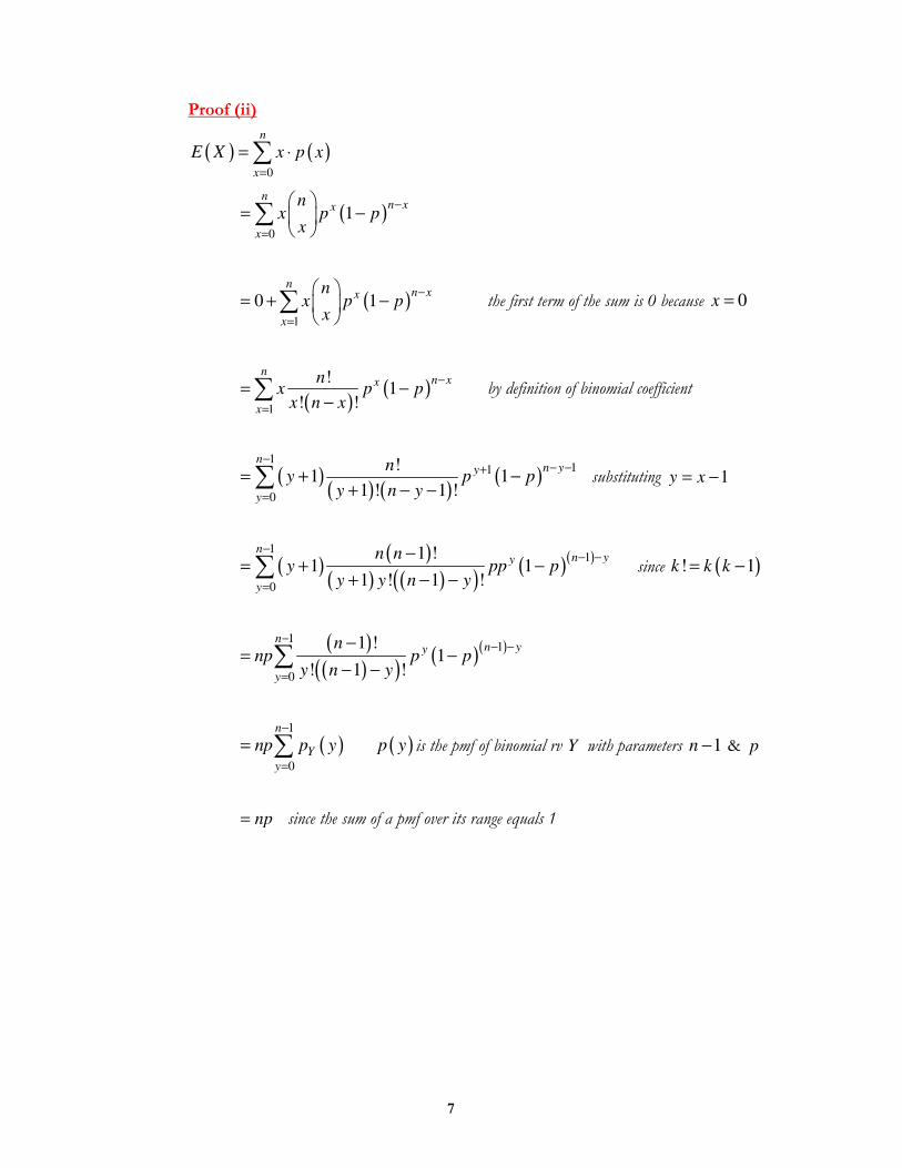
Proof (ii)

( ) ( )0

n

x

E X x p x=

= ⋅∑

( )0

1n

n xx

x

nx p p

x

−

=

= −

∑

( )1

0 1n

n xx

x

nx p p

x

−

=

= + −

∑ the first term of the sum is 0 because 0x =

( )( )

1

!1

! !

nn xx

x

nx p p

x n x

−

=

= −−

∑ by definition of binomial coefficient

( )( ) ( )

( )1

11

0

!1 1

1 ! 1 !

nn yy

y

ny p p

y n y

−− −+

=

= + −+ − −

∑ substituting 1y x= −

( )( )

( ) ( )( )( )( )

11

0

1 !1 1

1 ! 1 !

nn yy

y

n ny pp p

y y n y

−− −

=

−= + −

+ − −∑ since ( )! 1k k k= −

( )( )( )

( )( )1

1

0

1 !1

! 1 !

nn yy

y

nnp p p

y n y

−− −

=

−= −

− −∑

( )1

0

n

Y

y

np p y−

=

= ∑ ( )p y is the pmf of binomial rv Y with parameters 1n − & p

np= since the sum of a pmf over its range equals 1

8

Example 1 (Sample with replacement)

A certain kind of lizard lays 8 eggs, each of which will hatch independently with

probability 0.7. What is the probability that 3 eggs will hatch?

Solution

y 0 1 2 3 4 5 6 7 8

( )P Y y=

( )F y

4.4.1 Relation of Binomial to Bernoulli Distribution

(i) If ( )~ ,X Bin n p , with 1n = , then X has a Bernoulli distribution with

parameter p

( ) ( )1n xxn

p x p px

− = −

when 0 :x = ( ) ( ) ( )1 001

0 1 10

p p p p−

= − = −

when 1:x = ( ) ( )1 111

1 11

p p p p−

= − =

(ii) A binomial random variable can be viewed as the sum of n independent

Bernoulli random variables, one for each of the n independent

experiments that are performed.

9

4.5 Hyper-geometric Distribution

In chapter 1 we used sampling with and without replacement to illustrate the multiplication rules

for independent and dependent events. Analogous to that the binomial distribution, that applies

to sampling without replacement, in which case the trials are not independent.

Let us consider a set of N elements of which k are looked upon as successes and

the other N k− as failures. As in connection with the binomial distribution, we

are interested in the probability of getting x successes in n trials, but now we are

choosing, without replacement, n of the N elements contained in the set.

There are k

x

ways choosing xof the k successes and

N k

n x

−

− ways of choosing n x− of the N k− failures

Hence, k N k

x n x

−

− ways of choosing x successes and n x− failures;

There are N

n

ways of choosing n of the N elements in the set. We shall

assume that they are all equally likely.

Definition: A random variable X has a hypergeometric distribution if its

probability distribution is given by

( ) ( ) 0,1,2,....,

0 otherwise

k N k

x n xx n

Np x P X x

n

−

− == = =

Note: x k≤ and n x N k− ≤ −

10

Notation

(i). Let X have a hypergeometric distribution, that is, ( )~ ; , ,X HG x n N k

(ii). Let p k N= and 1q p= − ;

(a) ( )k

E X np nN

= =

(b) ( )1

N nVar X npq

N

− =

−

(iii). For N large: ( ) ( )1n xxn

P X x p px

− = −

� that is, if the element size N

is sufficiently large, the distribution of X may be approximated by the binomial

distribution.

Remark

� Note that the variance of X is somewhat smaller than the corresponding one

for the binomial case. The “correction term” ( ) ( )1 1N n N− − ≅ , for large N

� The approximation of the hypergeometric distribution to the binomial

distribution is very good if 0.1n N ≤ .

Example 1

Among the 120 applicants for a job, only 80 are actually qualified. If five of the

applicants are randomly selected for an interview, find the probability that only

two of the five will be qualified for the job by using

(a) Hypergeometric distribution

(b) Binomial approximation to hypergeometric

(c) Find the mean and variance

11

Solution

12

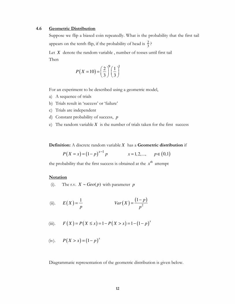
4.6 Geometric Distribution

Suppose we flip a biased coin repeatedly. What is the probability that the first tail

appears on the tenth flip, if the probability of head is 23?

Let X denote the random variable , number of tosses until first tail

Then

( )9 1

2 110

3 3P X

= =

For an experiment to be described using a geometric model,

a) A sequence of trials

b) Trials result in ‘success’ or ‘failure’

c) Trials are independent

d) Constant probability of success, p

e) The random variable X is the number of trials taken for the first success

Definition: A discrete random variable X has a Geometric distribution if

( ) ( )1

1x

P X x p p−

= = − 1,2,...,x = ( )0,1p ∈

the probability that the first success is obtained at the thx attempt

Notation

(i). The r.v. ~ ( )X Geo p with parameter p

(ii). ( )1

E Xp

= ( )( )

2

1 pVar X

p

−=

(iii). ( ) ( ) ( ) ( )1 1 1x

F X P X x P X x p= ≤ = − > = − −

(iv). ( ) ( )1x

P X x p> = −

Diagrammatic representation of the geometric distribution is given below.

13

Proof (iii)

( ) ( )XF x P X x= ≤

( ) 1

1

1x

i

i

p p−

=

= −∑

( ) 1

1

1x

i

i

p p−

=

= −∑

( )( )

1 1

1 1

xp

pp

− − = − −

(geometric series)

( )1 1x

p= − −

5 10 15 20

0.0

00.1

0

X~Geo(0.2):pmf

x

pro

b

5 10 15 20

0.0

00.1

5

X~Geo(0.5):pmf

x

pro

b

14

Proof (ii)

( )~X Geo p

( ) ( )1i

E X i P X i∞

=

= ⋅ =∑

( ) 1

1

1i

i

i p p∞

−

=

= ⋅ −∑

( ) 1

1

1i

i

p i p∞

−

=

= ⋅ −∑

( )

2

1

1 1

pp

= × − −

2

1p

pp⇒ =

( ) ( )2 2

1i

E X i P X i∞

=

= ⋅ =∑

( ) 12

1

1i

i

i p p∞

−

=

= ⋅ −∑

( ) 12

1

1i

i

p i p∞

−

=

= ⋅ −∑

( )

( )3

1 1

1 1

pp

p

+ −= ×

− −

3 2

2 2p pp

p p

− −⇒ =

( ) ( ) ( )2 2Var X E X E X= −

2 2 2

2 1 1p p

p p p

− −⇒ − =

15

Example 1

On a particular production line, the probability that an item is faulty is 0.08. In a

quality control test, items are selected at random from the production line. It is

assumed that quality of an item is independent of that of the other items.

(i). Find the probability that the first faulty item:

(a) does not occur in the first six selected,

(b) occurs in fewer than five selections.

(ii). If there is to be at least 90% chance of choosing a faulty item on or before

the thn attempt; What is the smallest numbern?

Solution

16

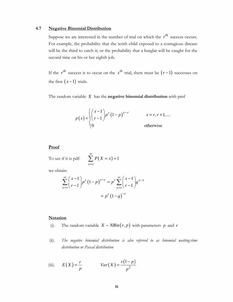
4.7 Negative Binomial Distribution

Suppose we are interested in the number of trial on which the thr success occurs.

For example, the probability that the tenth child exposed to a contagious disease

will be the third to catch it; or the probability that a burglar will be caught for the

second time on his or her eighth job.

If the thr success is to occur on the thx trial, there must be ( )1r − successes on

the first ( )1x − trials.

The random variable X has the negative binomial distribution with pmf

( )( )

11 , 1,....

1

0 otherwise

x rrxp p x r r

p x r

− − − = +

= −

Proof

To see if it is pdf: ( ) 1

x r

P X x∞

=

= =∑

we obtain:

( )1 1

11 1

x rr r x r

x r x r

x xp p p q

r r

∞ ∞− −

= =

− − − =

− − ∑ ∑

( )1rr

p q−

= −

Notation

(i). The random variable ( )~ ,X NBin r p with parameters p and r

(ii). The negative binomial distribution is also referred to as binomial waiting-time

distribution or Pascal distribution

(iii). ( )r

E Xp

= ( )( )

2

1r pVar X

p

−=

17

Example

If the probability is 0.35 that a child exposed to a certain contagious disease will

catch it, what is the probability that the tenth child exposed to the disease will be

the third to catch it?

Solution

4.7.1 Distributions relationship to the Negative Binomial

(i). Binominal

Let ( )~ ,X Bin n p , i.e. X = number of successes in n Bernoulli trials

with ( )P success p= .

Let ( )~ ,Y NBin r p , i.e. Y =number of Bernoulli trials required to obtain

r successes with ( )P success p= .

Then the following relationships hold:

(a) ( ) ( )P Y n P X r≤ = ≥

If there are r or more successes in the first n trials, then it

required n or fewer trials to obtain the first r successes.

(b) ( ) ( )P Y n P X r> = <

If there are fewer than r successes on the first n trials, then it

takes more than n trials to obtain r successes.

18

For example, suppose we wish to evaluate the probability that more than

10 repetitions are necessary to obtain the third success when 0.2p =

( ) ( ) ( ) ( )2

10

0

1010 3 0.2 0.8 0.678

r r

r

P Y P Xr

−

=

> = < = =

∑

The contrast between the both distributions, which involves repeated

Bernoulli trials: the binomial distribution arises when we deal with fixed

number say n , of such trials and are concerned with the number of

successes which occur. The negative binomial, is encountered when we

pre-assign the number of successes to be obtained and then record the

number of Bernoulli trials required.

(ii). Geometric

This a negative binomial distribution with parameter 1r = ; that is,

The pmf is ( ) ( )1

11

x rrxP X x p p

r

−− = = −

−

when 1:r = ( ) ( ) ( )1 1111 1

0

x xxp x p p p p

− −− = − = −

19

4.8 Poisson Distribution

Consider these random variables

� The number of emergency calls received by an ambulance control in an hour

� The number of vehicles approaching a motorway toll bridge in a five-minute

interval

� The number of flaws in a metre length material

� The number of bacteria in a litre of tainted water

Assuming each occur randomly, these are examples that can be modelled by the

Poisson distribution.

Conditions for Poisson model

(i). Events occur singly and at random in a given interval of time or space

(ii). λ , the mean number of occurrences per unit time is known and is finite.

The random variable X is the number of occurrences in the given interval.

If the above conditions are satisfied, X is said to follow a Poisson distribution,

with probability mass function

( ) ( ) 0,1,2,.....

!

0 otherwise

xe

xp x P X x x

λλ − =

= = =

Notation

(i). The random variable ( )~X Po λ with parameter λ , 0λ >

(ii). ( )E X λ= ( )Var X λ=

20

Proof

To check that ( )p x is a probability distribution

( )0 0

!

x

x x

P X x ex

λλ∞ ∞−

= =

= =

∑ ∑

0

!

x

x

ex

λ λ∞−

=

=

∑

1e eλ λ−⇒ =

Recall the Taylor series expansion of the exponential function

2 3

0

11! 2! 3! !

k

k

ek

λ λ λ λ λ∞

=

= + + + + = ∑…

Proof (ii)

( ) ( )0x

E X x P X x∞

=

= ⋅ =∑

0

!

x

x

ex

x

λλ−∞

=

= ⋅∑

( )1

01 !

x

x

e

x

λλ−∞

=

= +−

∑

1

0!

k

k

e

k

λλ+−∞

=

= ∑ letting 1k x= −

1

0!

k

k

e

k

λλ+−∞

=

= ∑

0

1

!

k

k

e

k

λλλ λ

−∞

=

=

⇒ =∑�����

21

( ) ( )2 2

0x

E X x P X x∞

=

= ⋅ =∑

2

0!

x

x

ex

x

λλ −∞

=

= ⋅∑

( )1

01 !

x

x

ex

x

λλ −∞

=

= + ⋅−

∑

( )1

0

1!

k

k

ek

k

λλ + −∞

=

= + ⋅∑ letting 1k x= −

2

0 0

1

! !

k k

k k

e ek

k k

λ λ

λ

λ λλ λ λ

− −∞ ∞

= =

= =

⇒ + = +

∑ ∑����� �����

( ) ( ) ( )2 2 2 2Var X E X E X λ λ λ λ= − = + − =

22

Example 3

On average, a school photocopier breaks down eight times during the school

week (Mon to Fri). Assuming that, the number of breakdowns can be modelled by

a Poisson distribution; find the probability that it breaks down

(i). Five times in a given week

(ii). Once on Monday

(iii). Eight times in a fortnight

Solutions

23

4.8.1 The Poisson distribution as an Approximation to Binomial

Let ( )~ ,X Bin n p ; and put ( )E X npλ = = and let n increase and p decrease

so that, λ remains constant.

Thus

( ) ( )1n xxn

P X x p px

− = = −

0,1,2,...,x n=

Letting p nλ= :

( ) 1

x n xnP X x

x n n

λ λ−

= = −

( )

!1

! !

x n xn

x n x n n

λ λ−

= −

−

( )

( )

( )

1!

! ! 1

nx

x x

nn

x n n x n

λλ

λ

−= ⋅ ⋅

− −

( ) ( ) ( )

( )

1 2 11

! 1

nx

x

n n nn n x

x n n n n n

λλ

λ

− − −− += ⋅ ⋅ ⋅ ⋅

−�

1 1 1 1! 1

x e

x

λλ −

⇒ × × × × × ×� as n → ∞

!

x

ex

λλ −=

When n is large ( 50n > ) and p is small, say, 0.1p < ; then the binomial

distribution ( )~ ,X Bin n p can be approximated using a Poisson distribution

with mean npλ = , i.e. ( )~X Po np

24

Example 1

Apples are packed into boxes each containing 250. On average, 0.6% of the apples

are found to be bad. Find, correct to two significant figures, the probability that

there will be more than two bad apples in a box.

Solution

25

4.8.2 Recursive formula to Poisson

In general

( )( )

1

11 !

re

P X rr

λλ− +

= + =+

( )1 !

re

r r

λλ λ−

= ×+

( )

( )1

P X rr

λ= × =

+

Suppose a typist makes errors at random and on average makes two errors per

page. Find the probability more than three errors on any given page.

Let the rv X denote the number errors made on a page, then ( )~ 2X Po

( ) ( )3 1 3 0.1429P X P X> = − ≤ =

( )P X x= ( )1P X r= +

( )0

2 20 0.1353

0!P X e

−= = = ( )0

2 20 0.1353

0!P X e

−= = =

( )2 12

1 0.27071!

eP X

−

= = = ( ) ( )2

1 0.1353 0.27071

P X = = =

( )2 22

2 0.27072!

eP X

−

= = = ( ) ( )2

2 0.2706 0.27062

P X = = =

( )2 32

3 0.18043!

eP X

−

= = = ( ) ( )2

3 0.2706 0.18043

P X = = =

This gives a considerable saving time, particularly when using a calculator.