chapitre 1 - icalde
TRANSCRIPT
NATIONAL HIGHER SCHOOL OF ENGINEERING YAOUNDE
Course support
DIGITAL IMAGE PROCESSING
Narcisse TALLA, PhD [email protected]
September 2015

Digital Image Processing National Higher School of Engineering 2015
By: Narcisse TALLA, [email protected]
i
TABLE DES MATIERES
TABLE DES MATIERES ..................................................................................................................................... I
CHAPTER1. FUNDAMENTALS ON DIGITAL IMAGE ............................................................................... 1
1.1 OBJECTIVES AND LEARNING OUTCOMES ........................................................................................................ 1 1.2 DEFINITION .................................................................................................................................................... 1 1.3 DIGITAL IMAGE ACQUISITION PRINCIPLE ........................................................................................................ 2
1.3.1 Principle ................................................................................................................................................. 2 1.3.2 Sensors functioning ................................................................................................................................ 3
1.4 DIGITAL IMAGE REPRESENTATION .................................................................................................................. 4 1.5 HEADER FILES ................................................................................................................................................ 5 1.6 MONO BAND AND MULTI BAND IMAGES ......................................................................................................... 6 1.7 EXERCISES ..................................................................................................................................................... 8
CHAPTER 2. READING AND DISPLAYING AN IMAGE .......................................................................... 10
2.1 OBJECTIVE ................................................................................................................................................... 10 2.2 READING AND DISPLAYING 8-BITS FORMAT IMAGES .................................................................................... 11
2.2.1 Pixel by pixel method ........................................................................................................................... 11 2.2.2 Line per Line method ........................................................................................................................... 12 2.2.3 Global method ...................................................................................................................................... 13
2.3 READING AND DISPLAYING A ZONE OF INTEREST IN AN 8-BITS FORMAT IMAGES .......................................... 13 2.3.1 Reading and displaying a ZOI using the Pixel by pixel method ........................................................... 14 2.3.2 Reading and displaying a ZOI using the Line by Line method............................................................. 15 2.3.3 Reading and displaying a ZOI using the global method ...................................................................... 15
2.4 READING AND DISPLAYING 16-BITS FORMAT IMAGES .................................................................................. 16 2.4.1 Conversion of images from 16-bits to 8-bits format. ............................................................................ 16
2.4.1.1 Conversion of 16-bits images in amplitude ..................................................................................................... 16 2.4.1.2 Reading and displaying a zone of interest in a 16-bits images in amplitudes .................................................. 17 2.4.1.3 Conversion of 16-bits images in intensities (PRI images) ............................................................................... 18
2.5 EXERCISES ................................................................................................................................................... 19
CHAPITRE 3. IMAGE CONVOLUTION WITH A LINEAR MASK .......................................................... 21
3.1 INTRODUCTION ............................................................................................................................................ 21 3.2 DIGITAL IMAGE CONVOLUTION PRINCIPLE ................................................................................................... 21 3.3 CASE OF IMAGE BORDER PIXELS ................................................................................................................... 24
3.3.1. Principle .............................................................................................................................................. 24 3.3.2 Zero’s method ...................................................................................................................................... 25 3.3.3 Symmetric method ................................................................................................................................ 25 3.3.4 Circular symmetric method .................................................................................................................. 25
3.4 EXERCISES ................................................................................................................................................... 26
CHAPTER 4 THE FILTERING OF IMAGES ................................................................................................ 27
4.1 INTRODUCTION ............................................................................................................................................ 27 4.2 LINEAR FILTERING ....................................................................................................................................... 27
4.2.1 Filters defined in 2-directions ....................................................................................................... 28 4.2.2 Filters defined in 4-directions ....................................................................................................... 28 4.2.3 Application .................................................................................................................................... 29
4.3 FILTERING OF THE GLISTENING ON SAR IMAGES ......................................................................................... 30 4.3.1 Preliminary .......................................................................................................................................... 30 4.3.2 local statistics ....................................................................................................................................... 31

Digital Image Processing National Higher School of Engineering 2015
By: Narcisse TALLA, [email protected]
ii
4.3.3 Glistening Standard Deviation estimation ........................................................................................... 31 4.3.4 LEE Filter of local statistics................................................................................................................. 32 4.3.5 Alternated Lee filter ............................................................................................................................. 34 4.3.6 Maximum of Probability a Posteriori (MAP) filter .............................................................................. 35 4.3.7 Gamma filter ........................................................................................................................................ 37 4.3.8 Frost filter ............................................................................................................................................ 38
4.4 APPLICATION ............................................................................................................................................... 40 4.5. EXERCISE ............................................................................................................................................... 42
CHAPTER 5. THE MATHEMATICAL MORPHOLOGY APPLIED TO IMAGES ................................. 43
5.1 INTRODUCTION ............................................................................................................................................ 43 5.2 IMAGE BINARISATION ................................................................................................................................... 43
5.2.1 Algorithm of image binarisation .......................................................................................................... 44 5.2.2 Example ................................................................................................................................................ 44
5.3 THE EROSION OF A BINARY IMAGE ............................................................................................................... 44 5.4 THE DILATION OF A BINARY IMAGE .............................................................................................................. 46 5.5 THE OPENING OF A BINARY IMAGE ............................................................................................................... 47 5.6 THE CLOSURE OF A BINARY IMAGE ............................................................................................................... 48 5.7 THE TOP HAT FORM ...................................................................................................................................... 49 5.8 IMAGE SKELETISATION ................................................................................................................................. 49
CHAPTER 6. TEXTURE ANALYSIS .............................................................................................................. 54
6.1 INTRODUCTION ............................................................................................................................................ 54 6.2 FIRST ORDER STATISTICAL METHODS ........................................................................................................... 54
6.2.1. Definition ............................................................................................................................................ 54 6.2.2 Examples of first order statistical parameters ..................................................................................... 54 6.2.3. Illustration ........................................................................................................................................... 55
6.3 SECOND ORDER STATISTICAL METHODS ....................................................................................................... 56 6.3.1 Definition ............................................................................................................................................. 56 6.3.2 Co-occurrence matrix .......................................................................................................................... 57 6.3.3 Image texture ........................................................................................................................................ 60
CHAPTER 7. IMAGE CLASSIFICATION ..................................................................................................... 68
7.1 INTRODUCTION ............................................................................................................................................ 68 7.2 CLASSIFICATION PROCESS ............................................................................................................................ 69
7.2.1 Classification protocol ......................................................................................................................... 69 7.2.2 Classification system ............................................................................................................................ 69 7.2.3 Training sites selection and statistics extraction .................................................................................. 70 7.2.4 Reduction of parameters ...................................................................................................................... 71
7.3 SUPERVISED IMAGE CLASSIFICATION ALGORITHMS ...................................................................................... 72 7.3.1 Parallelepiped method for image classification ................................................................................... 72 7.3.2 Minimum distance method for image classification ............................................................................. 73 7.3.3 K nearest neighbours method for image classification ........................................................................ 74 7.3.4 Maximum likelihood method for digital image classification .............................................................. 74
7.4 NON-SUPERVISED CLASSIFICATION ALGORITHMS ........................................................................................ 75 7.4.1 Histogram modes method for image classification .............................................................................. 76 7.4.2 ISODATA method for non-supervised image classification ................................................................. 78
7.5 NEURONAL NETWORKS METHOD FOR IMAGE CLASSIFICATION ..................................................................... 79 7.6 DETERMINATION OF CLASSIFICATION ACCURACY ........................................................................................ 79
7.6.1 Training and verification data ............................................................................................................. 79 7.6.2 Size of samples ..................................................................................................................................... 80 7.6.3 Sampling methods ................................................................................................................................ 80 7.6.4 Global precision and KAPPA coefficient ............................................................................................. 80

Digital Image Processing National Higher School of Engineering 2015
By: Narcisse TALLA, [email protected]
iii
CHAPTER 8. REMOTE SENSING IMAGE ANALYSIS .............................................................................. 82
8.1 INTRODUCTION ............................................................................................................................................ 82 8.2 TEXTURE TRANSFORMATIONS ...................................................................................................................... 82
8.2.1 Introduction .......................................................................................................................................... 82 8.2.2 Modeling by random process ............................................................................................................... 84
8.2.2.1. 2-D linear predicting model ........................................................................................................................... 84 8.2.2.2. Markov model ................................................................................................................................................ 84
8.2.3. Methods based on spatial characteristics ........................................................................................... 86 8.2.3.1. Generalised histograms of greyscales ............................................................................................................. 86 8.2.3.2. First order histogram-based method ............................................................................................................... 86 8.2.3.3. Second order histogram (co-occurrence matrix) method ................................................................................ 87
8.2.4. Algorithm for image texture calculation ............................................................................................. 91 8.2.5 Example of image texture calculation .................................................................................................. 92
8.2.5.1: Image window extraction ............................................................................................................................... 93 8.2.5.2: Calculation of the co-occurrence matrix ........................................................................................................ 93 8.2.5.3: Calculation of the texture parameter for extracted image window ................................................................. 93 8.2.5.4: Calculation of the image texture .................................................................................................................... 93 8.2.5.5. Normalisation of the image texture ................................................................................................................ 94 8.2.6 Third order statistical parameters ....................................................................................................................... 94
8.3 VEGETATION INDICES................................................................................................................................... 96

Digital Image Processing National Higher School of Engineering 2015
By: Narcisse TALLA, [email protected] 1
CHAPTER1. FUNDAMENTALS ON DIGITAL IMAGE
1.1 Objectives and learning outcomes
The goal of this chapter is to present the context and basic notions on digital image
processing, and remote sensing images in particular. By the end of the chapter, every
student must be able to:
1. Define and characterise a digital image;
2. Define and characterise a pixel;
3. Define and characterise image sensors;
4. Present the digital image acquisition principle;
5. Compare an 8-bits with a 16-bits format image;
6. Compare a monoband with a multiband image;
1.2 Definition
In general, an image is an information carrier. It has the elements of a scene that was
captured by either a camera or a satellite. Remote sensing images are generally derived
from onboard satellite sensors, and sometimes aerial photographs. An image can have
different definitions depending on the context. In signal processing, an image is defined
as a two-dimensional signal. Mathematically, an image is a real application IMG defined
as follows:
IRXIRIRNMIMG )(: (1.1)
In case of digital images, the subset (MxN) consists of pairs of integers (x,y), with
x NC 0 1 2, , . . . . . , and y NL 0 1 2, , . . . . . , where NL and NC represent respectively the
number of lines and columns of the image. So, a digital image is finally a matrix made of
NL lines and NC columns. Each cell of this matrix is an object point called pixel, acronym
of “picture element”, and the coordinates of the cell are the coordinates of the object point
in the observed region.

Digital Image Processing National Higher School of Engineering 2015
By: Narcisse TALLA, [email protected] 2
1.3 Digital image acquisition principle
1.3.1 Principle
Three components are involved in the digital image acquisition principle:
The object for which the image is taken;
A source that generates radiations;
A sensor that observes the object.
The following figure illustrates the digital image acquisition principle.
Figure 1.1. Digital Image acquisition principle
(1): The source, that can be the Sun, in case of an optical remote sensing image, illuminates
the object with electromagnetic radiations;
(2): The object, that can be a region of the Earth, reflects totally or in part the received
radiation towards the sensor;
(3): The Sensor, that can be on-board of a satellite, quantifies the received radiation from
the object and sends the value to the Space agency for registration.
During the process of quantification, if the maximum value a radiation can take is 255, we
talk of 8-bits image and each pixel of the image is coded on one byte. In case a radiation
value can reach 65535, we talk of 16-bits image and each pixel of the image can be coded
on 2 bytes.
The space Agency is equipped with a magnetic band which registers sequentially and
progressively data sent by the sensor in the form of bytes. This registration is done pixel
after pixel and line after line.

Digital Image Processing National Higher School of Engineering 2015
By: Narcisse TALLA, [email protected] 3
1.3.2 Sensors functioning
A sensor is an equipment that possesses an analogical to numerical and/or a numerical to
analogical converter of signals. Each sensor is sensitised to a certain range of signal
frequencies characterised by a minimum value fmin called low frequency and a maximum
value fmax called high frequency of the sensor. Only the radiations with frequencies
between fmin and fmax are detectable by this sensor. The frequency difference ∆f=fmax-fmin
is called spectral resolution of the sensor. The smaller this difference is, the higher the
spectral resolution is.
The sensor is made of a certain number of synchronised detectors with the same spectral
resolution. Each detector observes a specific point on the object. This point of a certain
surface is called pixel and its superficies is called spatial resolution. At a time (clock –
top), one line of the image is taken by these detectors and registered. So, an image of NL
lines is taken in NL clock-tops. If the sensor has NC detectors, then the image has NC
columns. In fact, each detector observes one column of the image. This is why a digital
image is finally a matrix.
The following table presents some sensors with their characteristics.
Table 1.1 Examples of sensors with some characteristics.
Sensor Lunching
date
Altitude Spatial
Resolution
Dimension of
the Scene LANDSAT 5 (USA) March 1985 705 km 30 x 30 m2 185 x 172 km2 SPOT (France)
February 1986 822 km 20 x 20 m2 (10 x 10 m in
Panchromatic mode)
60 x 60 km2
RADARSAT (Canada)
November 1995 793 km 10, 25, 50 et 100 m
50 à 500 km2
ERS (Europ)
July 1991 785 km 25 x 25 m2 (12.5 x 12.5 in
PRI mode)
100 x 100 km2
JERS (Japan) February 1992 568 km 18 x 24 m2 75 x 75 km2 ESAR (USA) 1995 8 km 6 x 6 m2
The following table presents some sensors observing the Cameroon Country.
Table 1.2 Examples of sensors observing Cameroon
Sensor Frequency or
wavelength
Sensor Type Passing
Frequency
Disponibility
in Cameroon LANDSAT 5 (USA)
0.76 – 0.90 µm (IR) 1.55 – 1.75 µm (IRM) 10.4 – 12.5 µm (IRT) 2.08 – 2.35 µm (IRM)
Thematic Mapper (TM) (scanning radiometer)
16 days Partially (North Region)
SPOT (France)
0.50 – 0.59 µm (B) 0.61 – 0.68 µm (V)
HRV (High Resolution Visible)
3 to 26 days Partially (North Region)
Digital Image Processing National Higher School of Engineering 2015
By: Narcisse TALLA, [email protected] 4
0.79 – 0.89 µm (IR) 0.51 – 0.73 µm (Panchromatic)
(scanning radiometer)
RADARSAT (Canada)
5.3 Ghz (Bande C) 5.66 cm
Polarisation HH
RSO (active sensor)
16 days (3 days in Canada)
Total
ERS (Europ)
5.3 Ghz (Bande C) 5.66 cm
Polarisation VV
RSO (active sensor)
35 days Total
JERS (Japon)
0.52 – 0.60 µm (B) 0.63 – 0.69 µm (V) 0.76 – 0.86 µm (R) 0.76 – 0.86 µm (IR)
1.60 – 1.71 µm (IRM) 2.01 – 2.12 µm (IRM) 2.13 – 2.15 µm (IRM) 2.27 – 2.40 µm (IRM)
5.3 Ghz (Bande C) 5.66 cm
Polarisation VV
SOP (Passive Sensor)
SAR (Active Sensor)
44 days Partially
Localised (Kribi Region)
ESAR (USA) 5.3 Ghz (Band C) 5.66 cm
Polarisation VV
SAR (Active Sensor)
Localised (Douala Region)
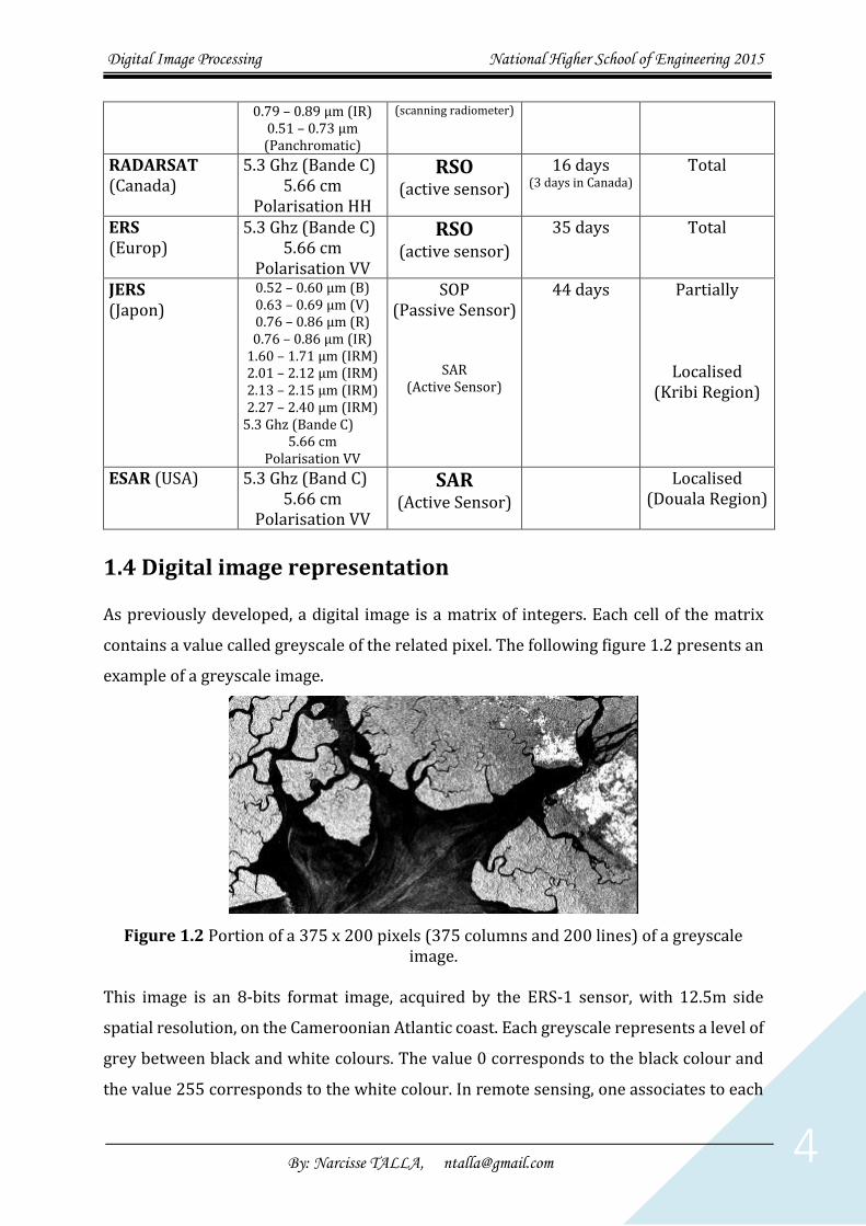
1.4 Digital image representation
As previously developed, a digital image is a matrix of integers. Each cell of the matrix
contains a value called greyscale of the related pixel. The following figure 1.2 presents an
example of a greyscale image.
Figure 1.2 Portion of a 375 x 200 pixels (375 columns and 200 lines) of a greyscale image.
This image is an 8-bits format image, acquired by the ERS-1 sensor, with 12.5m side
spatial resolution, on the Cameroonian Atlantic coast. Each greyscale represents a level of
grey between black and white colours. The value 0 corresponds to the black colour and
the value 255 corresponds to the white colour. In remote sensing, one associates to each
Digital Image Processing National Higher School of Engineering 2015
By: Narcisse TALLA, [email protected] 5
greyscale or range of greyscales a particular colour. This process is done by running an
algorithm similar to the following.
Algorithm 1.1 Image conversion from grayscales to colours
Input: Img: digital image;
T[1,..n]: Array of n thresholds of greyscales;
C[1,..n]: Array of n colours;
Output: Ima: coloured image (matrix of colours);
BEGIN
FOR each pixel (x,y) of the image Img, DO
IF ]1[),(Im0 Tyxg THEN Assign the colour C[1] to the cell Ima(x,y);
ELSEIF ]2[),(Im]1[ TyxgT THEN Assign the colour C[2] to the cell Ima(x,y);
---
ELSEIF 255][),(Im]1[ nTyxgnT THEN Assign the colour C[n] to the cell
Ima(x,y);
END;
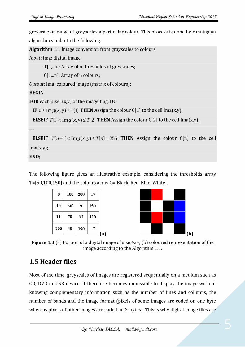
The following figure gives an illustrative example, considering the thresholds array
T=[50,100,150] and the colours array C=[Black, Red, Blue, White].
(a) (b)
Figure 1.3 (a) Portion of a digital image of size 4x4; (b) coloured representation of the image according to the Algorithm 1.1.
1.5 Header files
Most of the time, greyscales of images are registered sequentially on a medium such as
CD, DVD or USB device. It therefore becomes impossible to display the image without
knowing complementary information such as the number of lines and columns, the
number of bands and the image format (pixels of some images are coded on one byte
whereas pixels of other images are coded on 2-bytes). This is why digital image files are

Digital Image Processing National Higher School of Engineering 2015
By: Narcisse TALLA, [email protected] 6
always coupled with an additional file called header file. This file contains
complementary information required to display, analyse and interpret the image. Among
others, following are data contained in a header file: Orbital number, date of acquisition,
number of bands, image format (8-bits or 16-bits image), the number of columns and
lines, the geographical coordinates of the scene, the polarisation, the spectral and spatial
resolution, the name of the sensor, the altitude, etc. For a compressed image such as BMP,
JPG, GIF, PNG, TIF, GeoTiff etc., The header file and the image data are merged into a single
file in which a certain number of bytes generally at the beginning of the file are reserved
essential information of the header file.
1.6 Mono band and multi band images
On-board of some spatial engines (Satellite, Planes) are embarked many sensors, each
sensor possessing its proper spectral resolution, but all of them synchronised to take the
picture of the same object at the same moment. At the end of the acquisition process, for
a system of N sensors, the resulting image is made of N bands or channels. A band or
channel is the image of an object acquired by a sensor in a multi sensors system. In other
words, it is the image of an object acquired under a certain wavelength. A mono-band or
mono-channel image is then an image acquired by a system made of a single sensor. ERS-
1 or ERS-2 is an example of such a system. A multi-band or multi-channel image is an
image acquired by a system made of several sensors sensitised to different frequencies.
This is the case for example of Landsat5 and SPOT. The following illustrates a 3-bands
image acquired by the SPOT system.
Figure 1.4 A portion of size 180x180 pixels of a multi-band acquired by SPOT

Digital Image Processing National Higher School of Engineering 2015
By: Narcisse TALLA, [email protected] 7
This image of 20m size spatial resolution is part of Yaounde headquarters.
In fact, within a certain range of wavelength, two different objects can give the same
spectral answer. For example, a lake and a road can give the same spectral value if they
are observed under a certain wavelength. By changing the wavelength of sensor
sensibility, they can be discriminated. This is why a multi-band image gives more
information about the observed image than the mono-band image. But this fact has
nothing to do with the accuracy of the image which is improved as the spatial resolution
is higher.
Mathematically, a multi-band image can be defined as follows:
)),(),....,,(),,((),(
)(:
21 yxIyxIyxIyx
ININNMIMG
n
n
IR
(1.2)
In this equation, Ik(x,y) is the answer of the pixel at location (x,y) of the object to the kth
sensor of the system. Each pixel of the object has exactly n values.
At a time (clock-top), each sensor take the first line of the observed object and sends for
registration. i.e. if the image is made of NC columns then the first NC pixels of the magnetic
band constitute the first line of the first band; the NC following pixels constitute the first
line of the second band and progressively till the first line of the last band and the process
continues with the second line of the first band and similarly till the last line of the last
band.
In case of an 8-bits image, each byte of the magnetic band or medium represents one pixel.
But in case of a 16-bits image, each pixel is represented on the medium by a couple of
bytes.
Example: Let consider the following magnetic band representing a 4-band 16-bits image,
made of NC=4 columns and NL=2 lines.
Figure 1.5. A magnetic band
NB: The second line follows the first.
Solution:
Since it is a 16-bits image, each pixel is code on the magnetic band by a couple of bytes. So
the magnetic band which contains 64 bytes is made of 32 pixels.
Each band having 4 columns and two lines, each line is made of 4 pixels, i.e. 8 bytes. So the
first 8 bytes constitute the first line of the first band (Band A), the following 8 bytes

Digital Image Processing National Higher School of Engineering 2015
By: Narcisse TALLA, [email protected] 8
constitute the first line of the second band and progressively, we obtain the following
extracted bands:
Band A 1 0 1 56 2 0 1 1 1 1 2 2 3 2 2 1
Band B 1 200 2 100 2 200 0 200 0 3 1 1 2 1 2 2
Band C 0 100 0 99 2 10 1 1 0 2 0 1 0 1 2 0
Band D 2 2 3 2 2 1 0 3 1 1 0 3 1 1 0 3
Figure 1.6. Extracted bands
1.7 Exercises
What is a digital image?
What is the principle of image acquisition?
What is the spectral resolution of an image?
What is the spatial resolution of an image?
What is the difference between a spatial resolution and a spectral resolution?
How are image data stored on a medium?
What is the header file? What is its usefulness?
What is a mono-band image?
What is a multi-band image?
What is the usefulness of a multiband image?
Let consider the following image presented on figure 1.7.
Draw the equivalent image on a magnetic band;
Convert this image into a coloured image made of 5 colours, with thresholds: 50,
100, 150, 200 and 255.
Figure 1.7 A digital image of size 7x7 pixels.

Digital Image Processing National Higher School of Engineering 2015
By: Narcisse TALLA, [email protected] 9
Let consider the magnetic band of figure 1.6 of the previous example.
Extract the various bands, considering that instead of 4 columns and 2 lines, it is
now 2 columns and 4 lines;
Extract the various bands, considering that instead of 4 columns and 2 lines, it is
now 1 column and 8 lines;
Extract the various bands, considering that instead of 4 columns and 2 lines, it is
now 8 columns and 1 line;
Extract the various bands, considering that, instead of 4 bands, it is now 2 bands
and instead of 4 columns and 2 lines, it is now 4 columns and 4 lines.

Digital Image Processing National Higher School of Engineering 2015
By: Narcisse TALLA, [email protected] 10
CHAPTER 2. READING AND DISPLAYING AN IMAGE
2.1 Objective
This chapter aims to present various techniques of reading digital images from a medium
(Hard disk, CD, DVD…) and displaying on a region of a screen. The displaying can only be
possible when essential header file information such as the format of the image, and the
number of bands, lines and columns are known. In this chapter, we suppose that the
number of columns and lines of the image are known. By the end of this chapter, every
student should be able to:
Present the principle of reading and displaying an 8-bits format image pixel by
pixel;
Write an algorithm that reads, from a medium, an 8-bits format image and displays
on a given region of the computer screen pixel by pixel;
Present the principle of reading and displaying an 8-bits format image line by line;
Write an algorithm that reads, from a medium, an 8-bits format image and displays
on a given region of a computer screen line by line;
Present the principle of reading and displaying an 8-bits format image globally;
Write an algorithm that reads, from a medium, an 8-bits format image and displays
on a given region of a computer screen globally;
Present the principle of reading and displaying a zone of interest on an 8-bits
format image;
Write an algorithm that reads a region of interest from a medium and displays on
a given area of the computer screen;
Present the principle of converting a digital image from a 16-bits format (in
intensities or in amplitude) into an 8-bits format image;
Write an algorithm that converts a digital image from a 16-bits format (in
intensities or in amplitude) into an 8-bits format image;
Program all the previous algorithms in any programming language (Java,
C++Builder, Php, Matlab).

Digital Image Processing National Higher School of Engineering 2015
By: Narcisse TALLA, [email protected] 11
2.2 Reading and displaying 8-bits format images
The following figure illustrates the data storage mode, applied on the digital image of
figure 1.7.
Figure 2.1 Sequential representation of bytes of a digital image on a magnetic band.
Greyscales are stored on the magnetic band or data support (medium) sequentially,
starting from the first pixel of the first line till the last pixel of the last line. Once the
principle mastered, it is now easy to design an algorithm that reads an image from the
magnetic band and displays on a computer screen. In the following sections, we present
three methods of reading and displaying digital images. These methods are:
Pixel by pixel method;
Line by line method and
Global method.
In the following algorithms, the magnetic band is assimilated to a file of bytes.
2.2.1 Pixel by pixel method
This method consists in opening the file of bytes (image file), reading bytes successively
and displaying them as they are red. This method, in comparison with others is slow. This
is why it is no more implemented nowadays in most digital image processing softwares.
The strength of this method is that it requires les material (memory space). But the
material problem is no more up to date. The related algorithm is the following.

Digital Image Processing National Higher School of Engineering 2015
By: Narcisse TALLA, [email protected] 12
Algorithm 2.1 ReadDisplay_8bits_Pixel_By_Pixel Input: NL: Number of lines of the image; NC: Number of columns of the image; FileName: Name of the image file (File of bytes); Local variables: x , y: integer ;//Location of a pixel Pix: Byte; // to store temporarily each byte of the image BEGIN Open the image file named FileName; FOR y varying from 0 to NL-1 DO
FOR x varying from 0 to NC-1 DO BEGIN -Read one byte in the image file and store in Pix; -Display the colour corresponding to the value of Pix at the location (x,y) of the
screen; END Close the image file; END.
2.2.2 Line per Line method
This method consists in reading at once a line of the image and displaying the
corresponding colours. This process is repeated till the image is entirely read. For this
purpose, a variable of type Array of bytes is declared to store one line of the image each
time. The related algorithm is the following.
Algorithm 2.2 ReadDisplay_8bits_Line_per_Line Input: NL: Number of lines of the image; NC: Number of columns of the image; FileName: Name of the image file (File of bytes); Local variables: x , y: integer ;//Location of a pixel LB: Array of NC Bytes; // to store temporarily each line of bytes of the image BEGIN Open the image file named FileName; FOR y varying from 0 to NL-1 DO
BEGIN -Read one line of bytes in the image file and store in LB;
FOR x varying from 0 to NC-1 DO -Display the colour corresponding to the value of LB[x] at the location (x,y) of the
screen; END Close the image file; END.

Digital Image Processing National Higher School of Engineering 2015
By: Narcisse TALLA, [email protected] 13
The difference with the pixel by pixel method is that, instead of a single pixel, an entire
line of the image is read each time the image file is accessed. Experimentally, it has been
noticed that this method is at least twice faster than the pixel by pixel one.
2.2.3 Global method
This method consists in reading at once the entire image and displaying the image at the
relevant location. For this purpose, a variable of type Image is declared to store
temporarily the image during the process. This method is faster than the previous ones.
This is why it is used in most digital image processing softwares. The related algorithm is
the following.
Algorithm 2.3 ReadDisplay_8bits_Global Input: NL: Number of lines of the image; NC: Number of columns of the image; FileName: Name of the image file (File of bytes); Local variables: x , y: integer ;//Location of a pixel Bitmap: Array [0 .. NL-1, 0 .. NC-1] of Bytes; // to store temporarily the entire image BEGIN
Open the image file named FileName; FOR y varying from 0 to NL-1 DO FOR x varying from 0 to NC-1 DO Read one byte in the image file and store in Bitmap[y,x]; FOR y varying from 0 to NL-1 DO FOR x varying from 0 to NC-1 DO
Display the colour corresponding to the value of Bitmap[y,x] at the location (y,x) of the screen;
Close the image file; END.
2.3 Reading and displaying a zone of interest in an 8-bits format images
Sometimes, we are interested in reading and displaying just a portion of an image. This
portion is called Zone of Interest (ZOI). It is characterised by a starting point and an ending
point as shown in the following figure. In this case, the coordinates of the ending point of
the ZOI should be identified during the reading process of the image file.

Digital Image Processing National Higher School of Engineering 2015
By: Narcisse TALLA, [email protected] 14
Figure 2.2. Illustration of a zone of interest (ZOI) on a digital image.
In particular, one should notice that the file reader should be positioned on the byte
corresponding to the starting point of the ZOI. This starting point is the byte N°
(Y0*NC)+X0+1, (X0, Y0) being the coordinates of the starting point of the ZOI. The ZOI is an
image of X1-X0+1 columns and Y1-Y0+1 lines, (X1, Y1) being the coordinates of the ending
point of the ZOI. The reading and displaying of a ZOI can be done using one of the previous
methods.
2.3.1 Reading and displaying a ZOI using the Pixel by pixel method
Following is the algorithm of reading and displaying a ZOI using the pixel by pixel method:
Algorithm 2.4 ReadDisplay_ZOI_8bits_Pixel_By_Pixel Input: NL: Number of lines of the image; NC: Number of columns of the image; FileName: Name of the image file (File of bytes);
(X0, Y0), (X1, Y1): respectively the coordinates of the starting and ending points of the ZOI; Local variables: x , y: integer ;//Location of a pixel Pix: Byte; // to store temporarily each byte of the image BEGIN
Open the image file named FileName; FOR y varying from Y0 to Y1 DO BEGIN Place the file reader on the byte N° (y*NC)+Xo+1 in the image file; FOR x varying from 0 to X1-X0 DO
BEGIN Read one byte in the image file and store in Pix; -Display the colour corresponding to the value of Pix at the location (y-Y0, x)
of the screen; END
Close the image file; END.
Digital Image Processing National Higher School of Engineering 2015
By: Narcisse TALLA, [email protected] 15
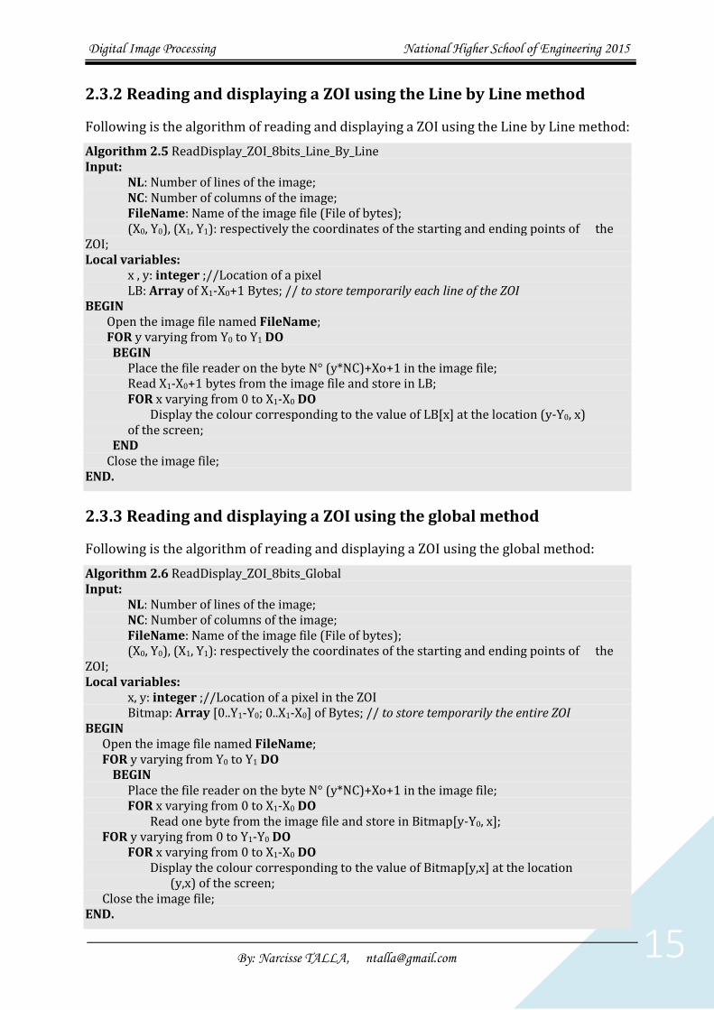
2.3.2 Reading and displaying a ZOI using the Line by Line method
Following is the algorithm of reading and displaying a ZOI using the Line by Line method:
Algorithm 2.5 ReadDisplay_ZOI_8bits_Line_By_Line Input: NL: Number of lines of the image; NC: Number of columns of the image; FileName: Name of the image file (File of bytes);
(X0, Y0), (X1, Y1): respectively the coordinates of the starting and ending points of the ZOI; Local variables: x , y: integer ;//Location of a pixel LB: Array of X1-X0+1 Bytes; // to store temporarily each line of the ZOI BEGIN
Open the image file named FileName; FOR y varying from Y0 to Y1 DO BEGIN
Place the file reader on the byte N° (y*NC)+Xo+1 in the image file; Read X1-X0+1 bytes from the image file and store in LB; FOR x varying from 0 to X1-X0 DO
Display the colour corresponding to the value of LB[x] at the location (y-Y0, x) of the screen;
END Close the image file;
END.
2.3.3 Reading and displaying a ZOI using the global method
Following is the algorithm of reading and displaying a ZOI using the global method:
Algorithm 2.6 ReadDisplay_ZOI_8bits_Global Input: NL: Number of lines of the image; NC: Number of columns of the image; FileName: Name of the image file (File of bytes);
(X0, Y0), (X1, Y1): respectively the coordinates of the starting and ending points of the ZOI; Local variables: x, y: integer ;//Location of a pixel in the ZOI Bitmap: Array [0..Y1-Y0; 0..X1-X0] of Bytes; // to store temporarily the entire ZOI BEGIN
Open the image file named FileName; FOR y varying from Y0 to Y1 DO BEGIN
Place the file reader on the byte N° (y*NC)+Xo+1 in the image file; FOR x varying from 0 to X1-X0 DO
Read one byte from the image file and store in Bitmap[y-Y0, x]; FOR y varying from 0 to Y1-Y0 DO
FOR x varying from 0 to X1-X0 DO Display the colour corresponding to the value of Bitmap[y,x] at the location
(y,x) of the screen; Close the image file;
END.

Digital Image Processing National Higher School of Engineering 2015
By: Narcisse TALLA, [email protected] 16
2.4 Reading and displaying 16-bits format images
In fact, a human eye cannot distinguish more than 256 colours (greyscales) between the
black and white colours. Since 16-bits images have more than 256 grayscales (65536
grayscales), it is therefore necessary to convert into an 8-bits image for displaying
purpose. After conversion, one of the three previous methods can be used to display the
image.
2.4.1 Conversion of images from 16-bits to 8-bits format.
Pixels of a 16-bits image have grayscales coded in the form of a complex number a+ib,
where a and b are integers varying from 0 to 255 each. Generally, one distinguishes two
categories of 16-bits images:
16-bits images in amplitudes;
16-bits images in intensities.
For images in intensities, the value of the grayscale Pix of a pixel is the intensity of the
complex number related to the pixel (Pix=a2+b2). This number can be greater than 255.
This is why it cannot be coded on a single byte but on two.
For images in amplitudes, the grayscale Pix of a pixel is the squawroot of the intensity of
the related complex number. It is also possible to obtain a 16-bits in amplitude from the
averages of complex number amplitudes. Grayscales of such images are already coded on
8-bits. In the following sections, we present the methods of converting each type of 16-
bits image into an 8-bits image.
2.4.1.1 Conversion of 16-bits images in amplitude
To convert a 16-bits image in amplitudes into an 8-bits image, some statistics are
required. Considering the image Img as a matrix of NL lines and NC columns, the Average
(AVG), the average of squares (AvgSq) and the Standard Deviation (SD) of data contained
in the matrix are given by the following equation.
{
𝐴𝑉𝐺 =
1
𝑁𝐿×𝑁𝐶∑ ∑ 𝐼𝑚𝑔[𝑦, 𝑥]𝑥=𝑁𝐶−1
𝑥=0𝑦=𝑁𝐿−1𝑦=0
𝐴𝑣𝑔𝑆𝑞 =1
𝑁𝐿×𝑁𝐶∑ ∑ (𝐼𝑚𝑔[𝑦, 𝑥])2𝑥=𝑁𝐶−1
𝑥=0𝑦=𝑁𝐿−1𝑦=0
𝑆𝐷 = √𝐴𝑣𝑔𝑆𝑞 − (𝐴𝑉𝐺)2
(Eq. 2.1)
The following algorithm converts an image from 16-bits in amplitudes to 8-bits.

Digital Image Processing National Higher School of Engineering 2015
By: Narcisse TALLA, [email protected] 17
Algorithm 2.7 Conversion16_8bits_amp Input: NL, NC: integers; //Respectively the number of lines and columns of the image; FileName: String; //Name of the 16-bits image file (file of bytes) Local Variables: x,y: integers ; // Coordinates of a pixel in the image LB: Array[1,--,2NC] of bytes; // Line of bytes IMA: Array[0,--,NL-1;0,--,NC-1] of reals; // to store temporarily the matrix image Output IM8: Array[0,--,NL-1; 0,--,NC-1] of bytes; // Converted image BEGIN
Open the image file named FileName; FOR y varying from 0 to NL-1 DO
BEGIN Read 2NC bytes in the image file and store in LB; FOR x varying from 0 to NC-1 DO
IMA[y,x] LB[2*x]*256+LB[2*x+1]; END
Calculate the statistics (AVG, AvgSq and SD) on data of the matrix IMA; FOR y varying from 0 to NL-1, DO
FOR x varying from 0 to NC-1, DO IM8[y,x] minimum{ENT((255*IMA[y,x])/(AVG + 3*SD)), 255};
Close the image file FileName; END
ENT represents the entire part.
Once converted from 16-bits to 8-bits, one can use any of the three basic methods to read
and display the converted image. Sometimes, we are not interested in the entire image,
but just in a portion of a 16-bits image. How do we process in this case?
2.4.1.2 Reading and displaying a zone of interest in a 16-bits images in amplitudes
Reading and displaying a zone of interest of a 16-bits image is similar to the case of an 8-
bits image. Following is the related algorithm.

Digital Image Processing National Higher School of Engineering 2015
By: Narcisse TALLA, [email protected] 18
Algorithm 2.8 Read_Display_ZOI_16bits_Amplitudes Input: NL, NC: integers; //Respectively the number of lines and columns of the image; FileName: String; //Name of the 16-bits image file (file of bytes) (X0,Y0), (X1,Y1): resp. the coordinates of the starting and ending pixels of the ZOI; Local Variables: x,y: integers ; // Coordinates of a pixel in the image a,b: integers; IMA: Array[0,--,X1-X0;0,--,X1-X0] of reals; // to store temporarily the matrix image Outputs: x ,y: de type entier ; IM8 : Array[0,--,Y1-Y0;0,--,X1-X0] of bytes; BEGIN
Open the image file named FileName; FOR y varying from Y0 to Y1, DO BEGIN Place the file reader on the byte N° 2*(y*NC+X0); FOR x varying from 0 to X1-X0, DO BEGIN Read 2 bytes from the image file and store respectively in a and b; IMA[y-Y0,x]a*256+b; END END Calculate the statistics (AVG, AvgSq and SD) on data of the matrix IMA; FOR y varying from 0 to Y1-Y0, DO
FOR x varying from 0 to X1-X0 DO IM8[y,x] minimum{ENT((255*IMA[y,x])/(AVG + 3*SD)), 255};
Close the image file FileName; IM8 contains the converted image that can be displayed using any of the three methods
developed above.
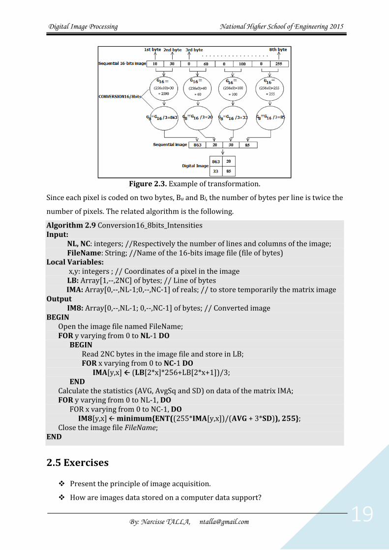
2.4.1.3 Conversion of 16-bits images in intensities (PRI images)
To convert an image from 16-bits in intensities to 8-bits, one should remember that the
value on 8 bits of each grayscale is a function of two consecutive bytes (upper and lower
bytes) in the image file. Before calculating the various statistics on the image, one should
first do the following transformation.
𝐺8 = [(256 ∗ 𝐵𝑢) + 𝐵𝑙]/3 (Eq. 2.2)
Where G8 is the grayscale of the pixel on 8-bits; Bu and Bl are respectively the upper-byte
of the lower-byte of the pixel. The following figure illustrates this transformation.
Digital Image Processing National Higher School of Engineering 2015
By: Narcisse TALLA, [email protected] 19
Figure 2.3. Example of transformation.
Since each pixel is coded on two bytes, Bu and Bl, the number of bytes per line is twice the
number of pixels. The related algorithm is the following.
Algorithm 2.9 Conversion16_8bits_Intensities Input: NL, NC: integers; //Respectively the number of lines and columns of the image; FileName: String; //Name of the 16-bits image file (file of bytes) Local Variables: x,y: integers ; // Coordinates of a pixel in the image LB: Array[1,--,2NC] of bytes; // Line of bytes IMA: Array[0,--,NL-1;0,--,NC-1] of reals; // to store temporarily the matrix image Output IM8: Array[0,--,NL-1; 0,--,NC-1] of bytes; // Converted image BEGIN
Open the image file named FileName; FOR y varying from 0 to NL-1 DO
BEGIN Read 2NC bytes in the image file and store in LB; FOR x varying from 0 to NC-1 DO
IMA[y,x] (LB[2*x]*256+LB[2*x+1])/3; END
Calculate the statistics (AVG, AvgSq and SD) on data of the matrix IMA; FOR y varying from 0 to NL-1, DO
FOR x varying from 0 to NC-1, DO IM8[y,x] minimum{ENT((255*IMA[y,x])/(AVG + 3*SD)), 255};
Close the image file FileName; END
2.5 Exercises
Present the principle of image acquisition.
How are images data stored on a computer data support?

Digital Image Processing National Higher School of Engineering 2015
By: Narcisse TALLA, [email protected] 20
Describe the various methods of reading and displaying digital images.
The figure 2.4 below represents a 16-bits image
o What are the number of lines and columns of this image, knowing that the
image has more than one line?
o Convert this image into an 8-bits image, considering that it is a 16-bits in
amplitude.
o Convert this image into an 8-bits image, considering that it is a 16-bits in
intensities.
o Identify on the 16-bits image the bytes of the ZOI starting from (1,1) and
ending on (3,3).
Write a program that reads, from a magnetic band (file of bytes) and displays on a
screen, an 8-bits image, using any programming language of your choice.
Write a program that converts a 16-bits image in amplitude into an 8-bits image,
using any programing language of your choice;
Write a program that converts a 16-bits image in intensities into an 8-bits image,
using any programing language of your choice;
Write a program that reads a zone of Interest (ZOI) from a 16-bits image and
displays on a computer screen.
0 27 3 1 0 0 1 191 2 3 0 1 0 32 1 0
1 2 3 0 1 125 4 0 0 44 2 136 2 3 1 165
Figure 2.4. a 16-bits image.
Digital Image Processing National Higher School of Engineering 2015
By: Narcisse TALLA, [email protected] 21
CHAPITRE 3. IMAGE CONVOLUTION WITH A LINEAR
MASK
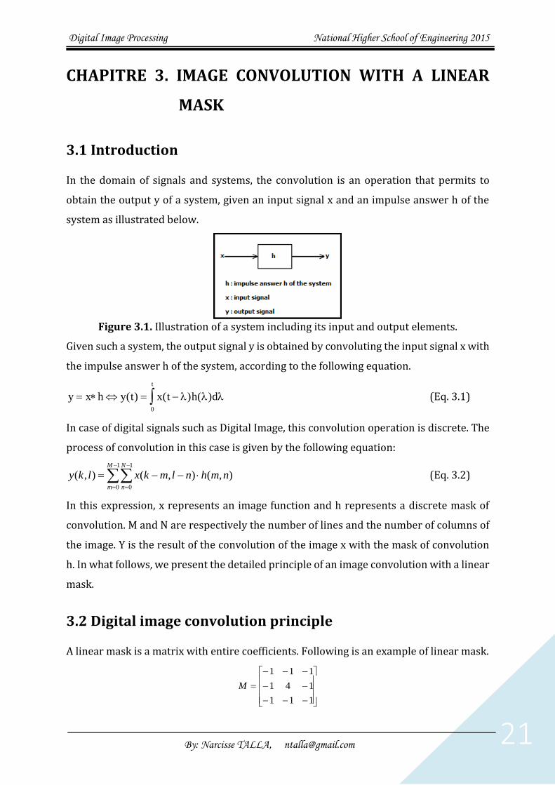
3.1 Introduction
In the domain of signals and systems, the convolution is an operation that permits to
obtain the output y of a system, given an input signal x and an impulse answer h of the
system as illustrated below.
Figure 3.1. Illustration of a system including its input and output elements.
Given such a system, the output signal y is obtained by convoluting the input signal x with
the impulse answer h of the system, according to the following equation.
y x h y t x t h d
t
( ) ( ) ( ) 0
(Eq. 3.1)
In case of digital signals such as Digital Image, this convolution operation is discrete. The
process of convolution in this case is given by the following equation:
1
0
1
0
),(),(),(M
m
N
n
nmhnlmkxlky (Eq. 3.2)
In this expression, x represents an image function and h represents a discrete mask of
convolution. M and N are respectively the number of lines and the number of columns of
the image. Y is the result of the convolution of the image x with the mask of convolution
h. In what follows, we present the detailed principle of an image convolution with a linear
mask.
3.2 Digital image convolution principle
A linear mask is a matrix with entire coefficients. Following is an example of linear mask.
111
141
111
M

Digital Image Processing National Higher School of Engineering 2015
By: Narcisse TALLA, [email protected] 22
The main steps of the linear convolution are the following:
1) Center the mask on each pixel of the image;
2) Calculate the linear combination of the coefficients of the mask with the grayscales of
the surrounding pixels of the central pixel of the image window (point on which the
mask is centred);
3) Replace the grayscale of the central point by the result of the previous combination.
4) Normalise the obtained result (convert the grayscales of the convoluted image in the
range of variation of grayscales of the original image).
For example, let consider the following image I and the previous mask M.
I
4 0 100 240
2 7 4 100
6 3 1 50
190 0 255 75 40
. . .
. . .
. . .
.
.
.
.
.
.
.
.
.
.
Let consider the point of coordinates (1,1) as our central point. Its grayscale is 7. This
point corresponds to the centre of the mask, the value 4. We can extract an image window
W from the digital image I and centred on the pixel (1,1).
136
472
10004
W
The surrounding points of the central point of the image window correspond to the values
-1 in the mask. The result of convolution is obtained by multiplying the two matrices
(image window and mask) term per term and the result replaces the central value of the
image window.
C = (-1 x 4)+(-1 x 0)+(-1 x 100)+(-1 x 2)+(4 x 7)+(-1 x 4)+(-1 x 6)+(-1 x 3)+(-1 x 1)
=-92.
At the end of the process, the results is normalised, using the following equation.
maxG
CGENTG old
new . (Eq. 3.3)
newG is the grayscale of the current pixel after normalisation. oldG is the maximum
grayscale in the original image. maxG is the maximum grayscale in the convoluted image
before normalisation and C is the value of the current convoluted pixel before
normalisation and ENT is the entire part operator.

Digital Image Processing National Higher School of Engineering 2015
By: Narcisse TALLA, [email protected] 23
For example, let suppose that the maximum grayscale of the convoluted image before
normalisation is 200 and that the maximum grayscale in the original image is 255. Then
the normalised convoluted pixel (1,1) of the previous image I is given by:
7315,72255
92200)1,1(
ENTENTG (Eq. 3.4)
The normalisation is necessary to visualise accurately the convoluted image and to better
appreciate the action of convolution on the image. The normalisation aims at bringing the
grayscales of the convoluted image in the range of variation of grayscales of the original
image so that one can better appreciate the changes operated by the convolution.
Following is an algorithm that convolutes an image with a linear mask.
Algorithm 3.1 Linear_Convolution Input: NL, NC: integers; //Respectively the number of lines and columns of the image; My, Mx: integers; //Respectively the number of lines and columns of the mask; IMG: Array[0--NL-1; 0--NC-1] of bytes; // Original image M: Array[0--My-1;0--Mx-1] of reals; // the linear mask; Local Variables: x,y: integers ; // Coordinates of a pixel in the image Output: IMA: Array[0,--,NL-1; 0,--,NC-1] of bytes; // Convoluted image BEGIN
FOR y varying from 0 to NL-1 DO FOR x varying from 0 to NC-1 DO
Convolution_Pixel(x, y, IMG, M, Mx, My, C); IMA[y,x] C ;
END //Normalisation Gmax Maximum value (grayscale) in IMA; Gold Maximum grayscale in IMG; FOR y varying from 0 to NL-1 DO
FOR x varying from 0 to NC-1 DO IMA[y,x] (IMA[y,x]* Gold)/Gold;
END
Convolution_Pixel is a sub-program that convolutes a single pixel (x,y) in an image IMG,
with a linear mask M of size Mx columns and My lines. The result is stored in the variable
C. Below is the specification of this sub-algorithm.
Algorithm 3.2 Convolution_Pixel Input: X0, Y0: integers; //coordinates of the pixel to convolute Mx, My: integers; //resp. number of columns and number of lines of the mask; IMG: Array[0--NL-1; 0--NC-1] of bytes; // Original image M: Array[0--My-1;0--Mx-1] of reals; // The linear mask
Digital Image Processing National Higher School of Engineering 2015
By: Narcisse TALLA, [email protected] 24
Local Variables: x,y: integers; // Coordinates of a pixel in the image I,J; Integers; Output C: integer; // Convoluted pixel BEGIN
C 0; FOR y varying from Y0-Wy/2 to Y0+Wy/2 DO
FOR y varying from X0-Wx/2 to X0+Wx/2 DO BEGIN
I x – Xo + (L/2); J y – Yo + (H/2); C C + (IMG[y,x] * M[J, I]);
END END
3.3 Case of image border pixels
3.3.1. Principle
The principle of image convolution cannot be applied on every point of the image, notably
the image border points. To make it possible, we have to add some virtual columns and
lines to the image so that, all the border points become internal points of the filled image.
The number of lines and columns depends on the size of the mask of convolution.
Considering a mask of size Mx columns and My lines, we can consider the point
(My/2,Mx/2) as the centre of the mask. In this case, we have to add ENT(Mx/2) empty
columns before the first column and ENT(Mx-1-(Mx/2)) empty columns after the last
column of the image. ENT being the entire part function. Similarly, we must add
ENT(My/2) empty lines before the first line and ENT(Mx-1-(My/2)) empty lines after the
last line of the image.
For example, with a mask of size 3 columns and 4 lines, the centre of the mask is the pixel
at coordinates (2,1). In this case, one must add 1 column before the first column, 1 column
after the last column, 2 lines before the first line and 1 line after the last line of the image.
Now that we know the number of empty columns and lines to add, the problem is how fill
them. For this purpose, there are various techniques of filling these empty points. But in
this chapter, we will present only three of them, notably the Zeros method, the symmetric
method and the circular symmetric method.
Digital Image Processing National Higher School of Engineering 2015
By: Narcisse TALLA, [email protected] 25
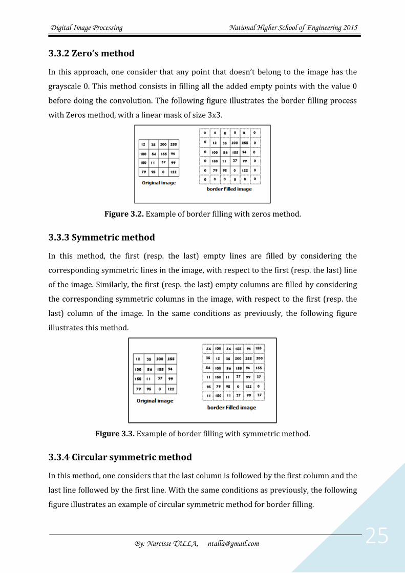
3.3.2 Zero’s method
In this approach, one consider that any point that doesn’t belong to the image has the
grayscale 0. This method consists in filling all the added empty points with the value 0
before doing the convolution. The following figure illustrates the border filling process
with Zeros method, with a linear mask of size 3x3.
Figure 3.2. Example of border filling with zeros method.
3.3.3 Symmetric method
In this method, the first (resp. the last) empty lines are filled by considering the
corresponding symmetric lines in the image, with respect to the first (resp. the last) line
of the image. Similarly, the first (resp. the last) empty columns are filled by considering
the corresponding symmetric columns in the image, with respect to the first (resp. the
last) column of the image. In the same conditions as previously, the following figure
illustrates this method.
Figure 3.3. Example of border filling with symmetric method.
3.3.4 Circular symmetric method
In this method, one considers that the last column is followed by the first column and the
last line followed by the first line. With the same conditions as previously, the following
figure illustrates an example of circular symmetric method for border filling.

Digital Image Processing National Higher School of Engineering 2015
By: Narcisse TALLA, [email protected] 26
Figure 3.4. Example of border filling with circular symmetric method.
3.4 Exercises
Describe the principle of image convolution.
What is the usefulness of border filling in image convolution?
Present the principle of the various methods of border filling.
Write a program in any programming language of your choice that convolutes a
digital image with a linear mask, using successively the three methods of border
filling.
Realise manually the convolution of the digital image defined in the following
figure, using the given mask and successively the three methods of border filling.
Figure 3.5. Digital image and the mask of convolution

Digital Image Processing National Higher School of Engineering 2015
By: Narcisse TALLA, [email protected] 27
CHAPTER 4 THE FILTERING OF IMAGES
4.1 Introduction
Satellite images often contain noise. This noise is due either to the surrounding nature, or
to the nature of the sensors embarked on the satellites. Such images often have a blurred
aspect. It is then necessary to filter them before any usage. Filters are classified in two
classes: linear filters and non-linear filters. SAR Images often contain a particular type of
noise called glistening. Only non-linear filters are suitable for the filtering of such images.
4.2 Linear filtering
Linear filtering consists in applying linear masks of convolution to the image. A linear
mask of classic filtering is for example the average mask M defined by: 𝑀 = [1 1 11 1 11 1 1
].
Filtering an image with the average filter consists in convoluting the image with the
average mask. The following image presents an example of SAR image filtered with the
average filter.
Figure 4.1. Example of linear filtering (average filter) realised on an ERS1 image of Kribi.
Linear masks are defined in two or four directions.
Digital Image Processing National Higher School of Engineering 2015
By: Narcisse TALLA, [email protected] 28
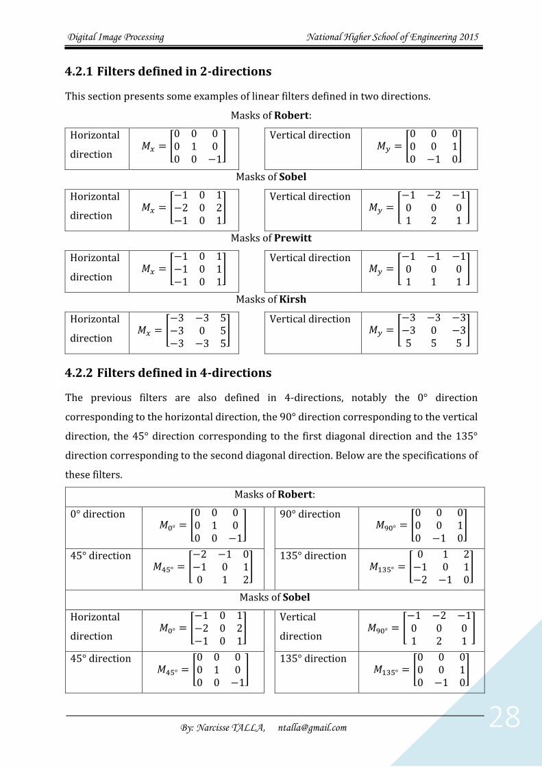
4.2.1 Filters defined in 2-directions
This section presents some examples of linear filters defined in two directions.
Masks of Robert:
Horizontal
direction 𝑀𝑥 = [
0 0 00 1 00 0 −1
] Vertical direction
𝑀𝑦 = [0 0 00 0 10 −1 0
]
Masks of Sobel
Horizontal
direction 𝑀𝑥 = [
−1 0 1−2 0 2−1 0 1
] Vertical direction
𝑀𝑦 = [−1 −2 −10 0 01 2 1
]
Masks of Prewitt
Horizontal
direction 𝑀𝑥 = [
−1 0 1−1 0 1−1 0 1
] Vertical direction
𝑀𝑦 = [−1 −1 −10 0 01 1 1
]
Masks of Kirsh
Horizontal
direction 𝑀𝑥 = [
−3 −3 5−3 0 5−3 −3 5
] Vertical direction
𝑀𝑦 = [−3 −3 −3−3 0 −35 5 5
]
4.2.2 Filters defined in 4-directions
The previous filters are also defined in 4-directions, notably the 0° direction
corresponding to the horizontal direction, the 90° direction corresponding to the vertical
direction, the 45° direction corresponding to the first diagonal direction and the 135°
direction corresponding to the second diagonal direction. Below are the specifications of
these filters.
Masks of Robert:
0° direction 𝑀0° = [
0 0 00 1 00 0 −1
] 90° direction
𝑀90° = [0 0 00 0 10 −1 0
]
45° direction 𝑀45° = [
−2 −1 0−1 0 10 1 2
] 135° direction
𝑀135° = [0 1 2−1 0 1−2 −1 0
]
Masks of Sobel
Horizontal
direction 𝑀0° = [
−1 0 1−2 0 2−1 0 1
] Vertical
direction 𝑀90° = [
−1 −2 −10 0 01 2 1
]
45° direction 𝑀45° = [
0 0 00 1 00 0 −1
] 135° direction
𝑀135° = [0 0 00 0 10 −1 0
]

Digital Image Processing National Higher School of Engineering 2015
By: Narcisse TALLA, [email protected] 29
Masks of Prewitt
Horizontal
direction 𝑀0° = [
−1 1 1−1 −2 1−1 1 1
] Vertical
direction 𝑀90° = [
−1 −1 −11 −2 11 1 1
]
45° direction 𝑀45° = [
−1 −1 1−1 −2 11 1 1
] 135° direction
𝑀135° = [1 1 1−1 −2 1−1 −1 1
]
Masks of Kirsh
Horizontal
direction 𝑀0° = [
−3 −3 5−3 0 5−3 −3 5
] Vertical
direction 𝑀90° = [
−3 −3 −3−3 0 −35 5 5
]
45° direction 𝑀45° = [
−3 −3 −3−3 1 5−3 5 5
] 135° direction
𝑀135° = [−3 5 5−3 0 5−3 −3 −3
]
4.2.3 Application
Let consider for example the image below acquired by ERS-1 on the Cameroonian Atlantic
coast.
Figure 4.2 Experimental image (ERS1 Cameroonian Atlantic coast image).
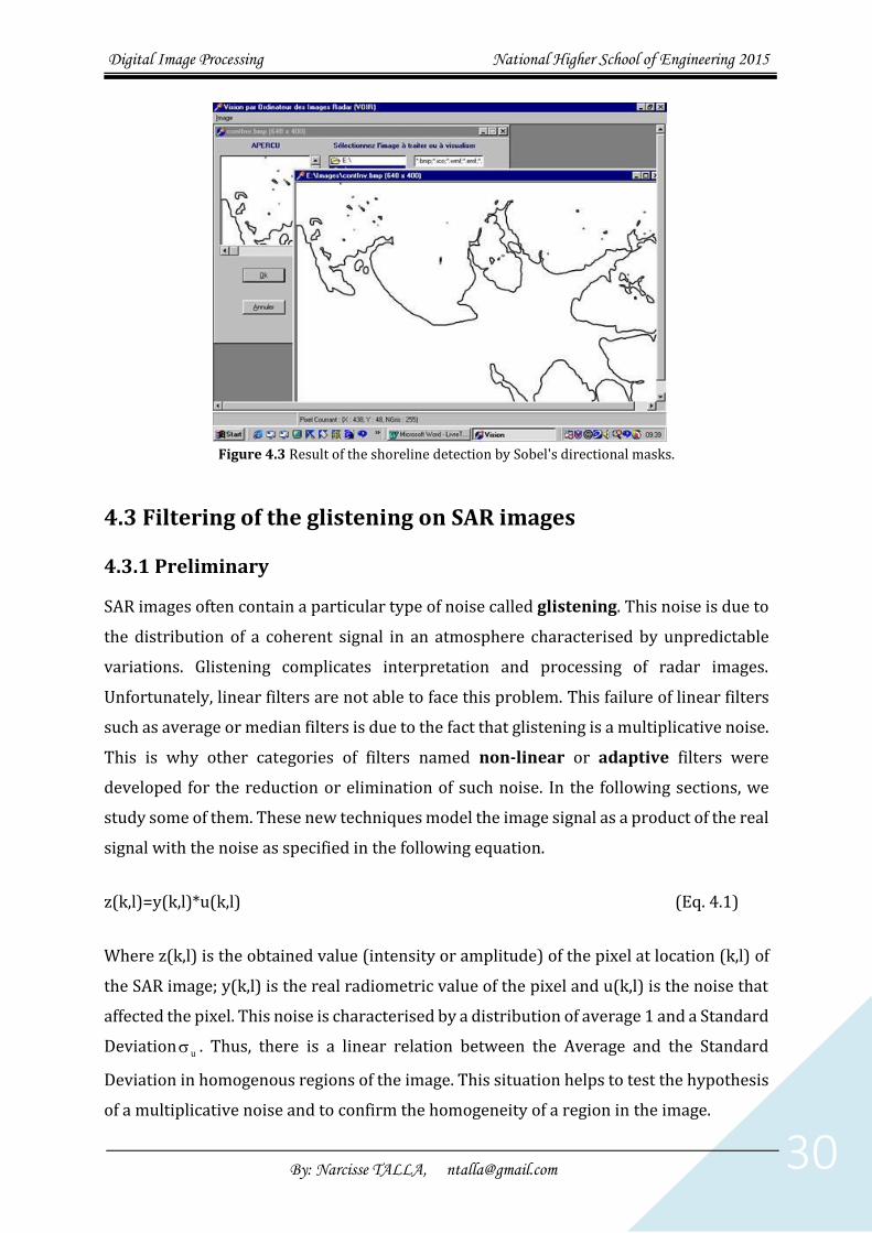
The image below presents the result of shoreline detection by filtering of the experimental
image with the Sobel’s directional filter. This result is obtained by convoluting the image
with each of the 4-directional masks of Sobel, notably 0°, 45°, 90° and 135° directions.
Each pixel of the experimental image is then convoluted 4 times. Finally, the value of the
filtered pixel is the maximum value of the 4 convolutions of the pixel. This value is
considered as the amplitude of the gradient of the considered pixel.
Digital Image Processing National Higher School of Engineering 2015
By: Narcisse TALLA, [email protected] 30
Figure 4.3 Result of the shoreline detection by Sobel's directional masks.
4.3 Filtering of the glistening on SAR images
4.3.1 Preliminary
SAR images often contain a particular type of noise called glistening. This noise is due to
the distribution of a coherent signal in an atmosphere characterised by unpredictable
variations. Glistening complicates interpretation and processing of radar images.
Unfortunately, linear filters are not able to face this problem. This failure of linear filters
such as average or median filters is due to the fact that glistening is a multiplicative noise.
This is why other categories of filters named non-linear or adaptive filters were
developed for the reduction or elimination of such noise. In the following sections, we
study some of them. These new techniques model the image signal as a product of the real
signal with the noise as specified in the following equation.
z(k,l)=y(k,l)*u(k,l) (Eq. 4.1)
Where z(k,l) is the obtained value (intensity or amplitude) of the pixel at location (k,l) of
the SAR image; y(k,l) is the real radiometric value of the pixel and u(k,l) is the noise that
affected the pixel. This noise is characterised by a distribution of average 1 and a Standard
Deviationu. Thus, there is a linear relation between the Average and the Standard
Deviation in homogenous regions of the image. This situation helps to test the hypothesis
of a multiplicative noise and to confirm the homogeneity of a region in the image.

Digital Image Processing National Higher School of Engineering 2015
By: Narcisse TALLA, [email protected] 31
4.3.2 local statistics
Since it is not possible to obtain an accurate model of the original signal, the image itself
can be used to estimate some required statistics, notably the Average and the Variance a
priori of the signal, based on the local Average and the local variance in an image window
of size n x n. From the multiplicative model of the noise, the following estimates of the
Average and the Variance a priori are obtained.
12
2222
u
uzy
s
szssandz
u
zy (Eq. 4.2)
We suppose that we have a linear filter expressed in the form where is the estimation of
the minimum of the squawroot of the signal y, a and b being chosen such as to minimize
the error in the least squares sense. It has been demonstrated that the best estimate of y
is given by the following equation.
zys
sbwithzzbzy
z
y ,)(~
2
2
(Eq. 4.3)
The unique input parameter of the filter is which depends on the SAR multi-view
treatment. It is necessary that should be always positive. Otherwise, it must be set to zero.
This problem can be escaped if a lower limit of regions homogeneity is conveniently
chosen. In the Lee original method, a linear model is introduced, with the optimal value of
b expressed in the following equation.
(Eq. 4.4)
By substitution, the following value of b is obtained:
(Eq. 4.5)
Knowing that , this linearisation doesn’t affect the filtering of glistening in the case of a 4-
views image in amplitude. But in the case of a 1-view SAR image, the exact expression
must be used. The estimation of the standard deviation of the noise is a function of the
number of views and a quality factor of the SAR image. Below is the algorithm that
estimates the Standard Deviation of the glistening.
4.3.3 Glistening Standard Deviation estimation
The estimation of the Standard Deviation of the noise is based on the Gamma function
given by the following algorithm.

Digital Image Processing National Higher School of Engineering 2015
By: Narcisse TALLA, [email protected] 32
Algorithm 4.1 Gamma_Function_Estimation: real;
-Input: N, integer representing the number of views of the image;
-Local variables: a, t: reals, k: integer;
BEGIN
a 1.7724538509; t 1; FOR k varying from 1 to N DO
t t*(2k–1); Return (a*t)/2N; END
With the Gamma function estimated, it is now possible to estimate the Standard Deviation
of the noise. The related algorithm is the following.
Algorithm 4.2. Noise_Standard_Deviation_Estimation: Real;
-Input: N: integer representing the number of views of the image;
Q: integer representing the factor or type of the image (Q=0 for 16-bits images in intensities; Q=1 for 8-bits images in amplitude of type squawroot of intensities; Q=2 for 8-bits n amplitudes of type average of amplitudes);
BEGIN
IF(Q = 0) THEN Noise_Standard_Deviation N1 ;
ELSEIF(Q = 1) THEN Noise_Standard_Deviation N273.0 ;
ELSEIF(Q = 2) THEN Noise_Standard_Deviation
1
!12
NGamma
NN
END
Following is the algorithm of Lee for the filtering of glistening on SAR images.
4.3.4 LEE Filter of local statistics
The following algorithm describes the process of filtering a SAR image affected by
glistening noise, using Lee filter.
Algorithm 4.3 Lee_Glistening_Filter
Input:
IMG: Original image;
NL, NC: integer representing respectively the number of lines and the number of
columns of the image IMG;
n: integer representing the size of the image window to consider;

Digital Image Processing National Higher School of Engineering 2015
By: Narcisse TALLA, [email protected] 33
Output:
IMA: Filtered image;
Local variables:
Imaf: Array[1..NL ; 1..NC] of reals;
i, j: integers;
a, b: reals;
BEGIN
1. Initialise the intermediary image table Imaf with the original image IMG;
2. FOR j varying from 0 to NL-1 DO
FOR i varying from 0 to NC-1 DO
BEGIN
a) Extract, from Imaf, an image window W centred on the pixel (i,j) ;
b) Calculate the local average
1
0
1
0
²],[n
a
n
b
nbaWz of W;
c) Calculate the local variance
1
0
1
0
2²],[1²1
n
a
n
b
fz zbaimanS of W;
d) Estimate the Standard Deviation of the noise in the image window:
{
𝑆𝑢 <− 𝑁𝑜𝑖𝑠𝑒_𝑆𝑡𝑎𝑛𝑑𝑎𝑟𝑑_𝐷𝑒𝑣𝑖𝑎𝑡𝑖𝑜𝑛(𝑁,𝑄) 𝑁: 𝑁𝑢𝑚𝑏𝑒𝑟 𝑜𝑓 𝑣𝑖𝑒𝑤𝑠 𝑜𝑓 𝑡ℎ𝑒 𝑖𝑚𝑎𝑔𝑒 𝑄: 𝐼𝑚𝑎𝑔𝑒 𝐹𝑎𝑐𝑡𝑜𝑟 𝑟𝑒𝑝𝑟𝑒𝑠𝑒𝑛𝑡𝑖𝑛𝑔 𝑡ℎ𝑒 𝑡𝑦𝑝𝑒 𝑜𝑓 𝑡ℎ𝑒 𝑖𝑚𝑎𝑔𝑒
e) Estimate the Average end the Variance a priori of the same image window:
y z
S S S Sy z u u
2 2 2 2
1
f) Verify the sign of the variance a priori:
0022 yy SThenSIf
g) Calculate the coefficient b:
bS
z S S
y
u y
2
2 2 2
h) Change the grayscale Imaf[i,j] by the following assignment:
],[Im jia f zjiabz f ],[Im ;
END
Digital Image Processing National Higher School of Engineering 2015
By: Narcisse TALLA, [email protected] 34
3. Transform the real values of Imaf into integers and assign to the image table IMA:
FOR j varying from 0 to NL-1 DO
FOR i varying from 0 to NC-1 DO
],[ jiIMA ],[Im jiaENT f ; ENT is the entire part function.
END
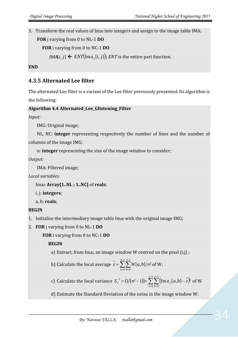
4.3.5 Alternated Lee filter
The alternated Lee filter is a variant of the Lee filter previously presented. Its algorithm is
the following:
Algorithm 4.4 Alternated_Lee_Glistening_Filter
Input:
IMG: Original image;
NL, NC: integer representing respectively the number of lines and the number of
columns of the image IMG;
n: integer representing the size of the image window to consider;
Output:
IMA: Filtered image;
Local variables:
Imaf: Array[1..NL ; 1..NC] of reals;
i, j: integers;
a, b: reals;
BEGIN
1. Initialise the intermediary image table Imaf with the original image IMG;
2. FOR j varying from 0 to NL-1 DO
FOR i varying from 0 to NC-1 DO
BEGIN
a) Extract, from Imaf, an image window W centred on the pixel (i,j) ;
b) Calculate the local average
1
0
1
0
²],[n
a
n
b
nbaWz of W;
c) Calculate the local variance
1
0
1
0
2²],[Im1²1
n
a
n
b
fz zbaanS of W
d) Estimate the Standard Deviation of the noise in the image window W:

Digital Image Processing National Higher School of Engineering 2015
By: Narcisse TALLA, [email protected] 35
{
𝑆𝑢 <− 𝑁𝑜𝑖𝑠𝑒_𝑆𝑡𝑎𝑛𝑑𝑎𝑟𝑑_𝐷𝑒𝑣𝑖𝑎𝑡𝑖𝑜𝑛(𝑁,𝑄) 𝑁: 𝑁𝑢𝑚𝑏𝑒𝑟 𝑜𝑓 𝑣𝑖𝑒𝑤𝑠 𝑜𝑓 𝑡ℎ𝑒 𝑖𝑚𝑎𝑔𝑒 𝑄: 𝐼𝑚𝑎𝑔𝑒 𝐹𝑎𝑐𝑡𝑜𝑟 𝑟𝑒𝑝𝑟𝑒𝑠𝑒𝑛𝑡𝑖𝑛𝑔 𝑡ℎ𝑒 𝑡𝑦𝑝𝑒 𝑜𝑓 𝑡ℎ𝑒 𝑖𝑚𝑎𝑔𝑒
e) Estimate the Standard Deviation a priori of the same image window:
1
)0(2
y
zy
SElse
zSSThenzIf
f) Compare the Standard deviation a priori with the Standard Deviation of the
noise and deduce the grayscale of the filtered pixel:
If (Sy < Su) Then
ima i j ENT z[ , ] ( )
ELSE
BEGIN
bENTijIMA
abb
SSzSSijab
SSa
uuuyf
uy
],[
],[Im4222
42
END
END
4.3.6 Maximum of Probability a Posteriori (MAP) filter
This adaptive filter is based on the maximisation of the probability a posteriori (MAP),
p(y/z) of the signal y(k,l), knowing z(k,l): . Given an N-look image in intensities, P(y/z)
follows thesquare:
In contrary to the Lee filter that doesn’t require any model for the signal, the MAP filter
supposes that the signal follows a Gaussian distribution: and being respectively the
Average and the Variance estim!€ated through local statistics in an image window. The
related algorithm is the following:

Digital Image Processing National Higher School of Engineering 2015
By: Narcisse TALLA, [email protected] 36
Algorithm 4.5 MAP_Glistening_Filter
Input:
IMG: Original image;
NL, NC: integer representing respectively the number of lines and the number of
columns of the image IMG;
n: integer representing the size of the image window to consider;
Output:
IMA: Filtered image;
Local variables:
Imaf: Array[1..NL ; 1..NC] of reals;
i, j: integers;
a, b: reals;
BEGIN
1. Initialise the intermediary image table Imaf with the original image IMG;
2. FOR j varying from 0 to NL-1 DO
FOR i varying from 0 to NC-1 DO
BEGIN
a) Extract, from Imaf, an image window W centred on the pixel (i,j) ;
b) Calculate the local average
1
0
1
0
²],[n
a
n
b
nbaWz of W;
c) Calculate the local variance
1
0
1
0
2²],[1²1
n
a
n
b
z zbaWnS of W;
d) Estimate the Standard Deviation of the noise in the image window W:
{
𝑆𝑢 <− 𝑁𝑜𝑖𝑠𝑒_𝑆𝑡𝑎𝑛𝑑𝑎𝑟𝑑_𝐷𝑒𝑣𝑖𝑎𝑡𝑖𝑜𝑛(𝑁,𝑄) 𝑁: 𝑁𝑢𝑚𝑏𝑒𝑟 𝑜𝑓 𝑣𝑖𝑒𝑤𝑠 𝑜𝑓 𝑡ℎ𝑒 𝑖𝑚𝑎𝑔𝑒 𝑄: 𝐼𝑚𝑎𝑔𝑒 𝐹𝑎𝑐𝑡𝑜𝑟 𝑟𝑒𝑝𝑟𝑒𝑠𝑒𝑛𝑡𝑖𝑛𝑔 𝑡ℎ𝑒 𝑡𝑦𝑝𝑒 𝑜𝑓 𝑡ℎ𝑒 𝑖𝑚𝑎𝑔𝑒
e) Estimate the Standard Deviation a priori of the same image window:
0
)0(2
y
zy
SElse
zSSThenzIf
f) Compare the Standard deviation a priori with the Standard Deviation of the
noise and deduce the grayscale of the filtered pixel:

Digital Image Processing National Higher School of Engineering 2015
By: Narcisse TALLA, [email protected] 37
If (Sy < Su) Then
ima i j ENT z[ , ] ( )
ELSE
BEGIN
abENTijIMA
SSzSSijab
SSa
yuuyf
uy
/],[
1],[Im
1
2222
22
END
END
4.3.7 Gamma filter
This filter is similar to the previous one, but takes into consideration the number of views
of the image to filter. Its algorithm is the following.
Algorithm 4.6 Gamma_Glistening_Filter
Input:
IMG: Original image;
NL, NC: integer representing respectively the number of lines and the number of
columns of the image IMG;
n: integer representing the size of the image window to consider;
Nviews: Number of the views of the image to filter;
Output:
IMA: Filtered image;
Local variables:
Imaf: Array[1..NL ; 1..NC] of reals;
i, j: integers;
a, b, t1, t2, t: reals;
BEGIN
1. Initialise the intermediary image table Imaf with the original image IMG;
2. FOR j varying from 0 to NL-1 DO
FOR i varying from 0 to NC-1 DO
BEGIN
a) Extract, from Imaf, an image window W centred on the pixel (i,j) ;

Digital Image Processing National Higher School of Engineering 2015
By: Narcisse TALLA, [email protected] 38
b) Calculate the local average
1
0
1
0
²],[n
a
n
b
nbaWz of W;
c) Calculate the local variance
1
0
1
0
2²],[1²1
n
a
n
b
z zbaWnS of W;
d) Estimate the Standard Deviation of the noise in the image window W:
{
𝑆𝑢 <− 𝑁𝑜𝑖𝑠𝑒_𝑆𝑡𝑎𝑛𝑑𝑎𝑟𝑑_𝐷𝑒𝑣𝑖𝑎𝑡𝑖𝑜𝑛(𝑁,𝑄) 𝑁: 𝑁𝑢𝑚𝑏𝑒𝑟 𝑜𝑓 𝑣𝑖𝑒𝑤𝑠 𝑜𝑓 𝑡ℎ𝑒 𝑖𝑚𝑎𝑔𝑒 𝑄: 𝐼𝑚𝑎𝑔𝑒 𝐹𝑎𝑐𝑡𝑜𝑟 𝑟𝑒𝑝𝑟𝑒𝑠𝑒𝑛𝑡𝑖𝑛𝑔 𝑡ℎ𝑒 𝑡𝑦𝑝𝑒 𝑜𝑓 𝑡ℎ𝑒 𝑖𝑚𝑎𝑔𝑒
e) Estimate the Standard Deviation a priori of the same image window:
0
)0(2
y
zy
SElse
zSSThenzIf
f) Compare the Standard deviation a priori with the Standard Deviation of the
noise and deduce the grayscale of the filtered pixel:
If (Sy² - Su²) 0 Then
BEGIN
2/],[
],[4
1
1
21
2
12
1
222
tENTjiIMA
ttt
zjiIMANtt
Nzt
SSS
fviews
views
uyu
END
END
4.3.8 Frost filter
This adaptive filter supposes that the useful information has an exponential auto-
correlation function. i.e. the image is stationary in a significant neighbourhood of the
filtered pixel. In this case, the best estimate of the signal is:
1
0
1
0
1 ),(~ 00
n
k
n
l
llkkalkzaky e where represents the coordinates of the central pixel of
the image window of size n x n, is the grayscale of the pixel located at (k,l), k1 is a
normalisation constant chosen to set the sum of filter weights to one. The constant a is

Digital Image Processing National Higher School of Engineering 2015
By: Narcisse TALLA, [email protected] 39
given by: , where is the normalisation constant, chosen to insure that . The Forst algorithm
specification is the following:
Algorithm 4.7 Frost_Glistening_Filter
Input:
IMG: Original image;
NL, NC: integer representing respectively the number of lines and the number of
columns of the image IMG;
n: integer representing the size of the image window to consider;
Nviews: Number of the views of the image to filter;
Output:
IMA: Filtered image;
Local variables:
IMAf: Array[1..NL ; 1..NC] of reals;
i, j: integers;
a, b, t1, t2, t: reals;
BEGIN
1. Initialise the intermediary image table Imaf with the original image IMG;
2. FOR j varying from 0 to NL-1 DO
FOR i varying from 0 to NC-1 DO
BEGIN
g) Extract, from IMAf, an image window W centred on the pixel (i,j) ;
h) Calculate the local average
1
0
1
0
²],[n
a
n
b
nbaWz of W;
i) Calculate the local variance
1
0
1
0
2²],[1²1
n
a
n
b
z zbaWnS of W;
j) Estimate the Standard Deviation of the noise in the image window W:
{
𝑆𝑢 <− 𝑁𝑜𝑖𝑠𝑒_𝑆𝑡𝑎𝑛𝑑𝑎𝑟𝑑_𝐷𝑒𝑣𝑖𝑎𝑡𝑖𝑜𝑛(𝑁,𝑄) 𝑁: 𝑁𝑢𝑚𝑏𝑒𝑟 𝑜𝑓 𝑣𝑖𝑒𝑤𝑠 𝑜𝑓 𝑡ℎ𝑒 𝑖𝑚𝑎𝑔𝑒 𝑄: 𝐼𝑚𝑎𝑔𝑒 𝐹𝑎𝑐𝑡𝑜𝑟 𝑟𝑒𝑝𝑟𝑒𝑠𝑒𝑛𝑡𝑖𝑛𝑔 𝑡ℎ𝑒 𝑡𝑦𝑝𝑒 𝑜𝑓 𝑡ℎ𝑒 𝑖𝑚𝑎𝑔𝑒
k) Calculate the following coefficient k: k n Su 42 ;
l) Calculate the following constant a: a k S zz 2 2
;
m) Execute the following assignment:

Digital Image Processing National Higher School of Engineering 2015
By: Narcisse TALLA, [email protected] 40
1
0
1
0
;],[],[n
m
n
l
X
f jlimaXwithlmWjiIMA e
END
3. Determine the maximum value IMAmax in IMAf;
4. FOR j varying from 0 to NL-1 DO
FOR i varying from 0 to NC-1 DO
IMAIMAf
ENTijIMA
max
255],[
END
4.4 Application
Let consider the following image of 3 lines and 3 columns (NL=3 and NC=3). Let filter this
image with the Lee filter, using an image window of size 3x3 and the symmetry principle
of border filling.
Figure 4.4 an example of digital image to filter.
The first pixel of this image is the pixel of coordinates (0,0), with grayscale 205. The image
window centred on this pixel, considering the symmetry border filling principle is the
following:
W205
174 215 174
242 205 242
174 215 174
1- The local average of this image window is calculated as follows:
z ( ) / ( ) .174 215 174 242 205 242 174 215 174 3 3 201 66
2- The local variance of W205 is calculated as follows:

Digital Image Processing National Higher School of Engineering 2015
By: Narcisse TALLA, [email protected] 41
S z
2174 201 66 215 201 66 174 201 66
242 201 66 205 201 66 242 201 66
174 201 66 215 201 66 174 201 66 9 1
6682 8 835 25
(( . )² ( . )² ( . )²
( . )² ( . )² ( . )²
( . )² ( . )² ( . )²) / ( )
/ .
3- Supposing that the image factor is Q=1 and that the number of views is 1, the Standard
Deviation of noise is calculated as follows: Su 0 273 1 0 5225. / .
4- The average and the variance a priori are given by:
y z
S S S Sy z u u
201 66
1 835 25 0 5225 0 5225 1 655 92 2 2 2
.
( . . ²) / ( . ² ) .
5- We notice that the variance a priori Sy
2 is positive, so nothing to change.
6- Let calculate the coefficient b:
bS
z S S
y
u y
2
2 2 2
655 9
201 66 0 5225 655 90 05578
.
. ² . ² ..
7- The value of IMAf[0,0] is then given by:
84.201)66.201205(05578.066.201],[],[ zijIMAbzijIMA ff
8- The entire part of 201.84 is 201. So the filtered value IMA[0,0] of IMG[0,0] is 201.
Similarly to what precedes, image windows centred on other pixels of the image are
presented in the following figure:
Figure 4.5 Different image windows centred on pixels of the original image of Figure 4.4.

Digital Image Processing National Higher School of Engineering 2015
By: Narcisse TALLA, [email protected] 42
Following the same process as previously for these image windows, the results of
intermediary calculus are presented in the table below.
Table 4.1. Intermediary results obtained during the Lee filtering process.
Window W242 W185 W174 W162 W144 W185 W215 W121
z 192.66 187.66 181.44 183.55 172.44 165.88 184.55 170.55
Sz
2 777.5 997 1357.77 1326.53 932.3 202.10 1937 983
Su 0.5225 0.5225 0.5225 0.5225 0.5225 0.5225 0.5225 0.5225
Sy
2 610.54 782.97 1066.4 1041.83 732 158.54 1521.4 771.97
b 0.05682 0.0753 0.1060 0.1017 0.0827 0.02067 0.1406 0.0886
],[ jiIMAf 195.46 187.46 180.65 181.35 170.08 166.27 188.83 166.15
],[ jiIMA 195 187 180 181 170 166 188 166
The following figure presents the final result of the filtering with the Lee filter.
Figure 4.6 Result of the Lee filtering of the digital image of figure 4.4.
No method of glistening filtering is absolutely better than another. Nevertheless, a given
method can be better than another for a particular application.
4.5. Exercise
What is the difference between a linear filter and a non-linear filter? Is one of the
two better than another one?
Consider the original image of figure 4.4 and the circular symmetry method.
o Filter this image with Sobel, Kirsh, Robert and Prewitt filters;
o Filter this image with Gama, MAP and Alternated Lee filter, considering
n=3, N=2 and Q=2.
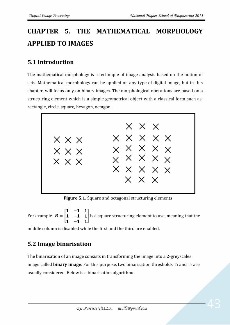
Digital Image Processing National Higher School of Engineering 2015
By: Narcisse TALLA, [email protected] 43
CHAPTER 5. THE MATHEMATICAL MORPHOLOGY
APPLIED TO IMAGES
5.1 Introduction
The mathematical morphology is a technique of image analysis based on the notion of
sets. Mathematical morphology can be applied on any type of digital image, but in this
chapter, will focus only on binary images. The morphological operations are based on a
structuring element which is a simple geometrical object with a classical form such as:
rectangle, circle, square, hexagon, octagon...
Figure 5.1. Square and octagonal structuring elements
For example 𝑩 = [𝟏 −𝟏 𝟏𝟏 −𝟏 𝟏𝟏 −𝟏 𝟏
] is a square structuring element to use, meaning that the
middle column is disabled while the first and the third are enabled.
5.2 Image binarisation
The binarisation of an image consists in transforming the image into a 2-greyscales
image called binary image. For this purpose, two binarisation thresholds T1 and T2 are
usually considered. Below is a binarisation algorithme

Digital Image Processing National Higher School of Engineering 2015
By: Narcisse TALLA, [email protected] 44
5.2.1 Algorithm of image binarisation
Algorithm 5.1 Binarisation
Input: IMG: greyscales image;
NC, NL: Number of Columns and Number of lines respectively;
T1, T2: classification threshold.
Output: IMA: binarised image of NL lines and NC columns;
Local variable: i,j: integers;
BEGIN
FOR j varying from 0 to NL-1 DO
FOR i varying from 0 to NC-1 DO
IF (IMG[i, j]≥T1) and (IMG[i, j]≤T2) THEN IMA[i, j]←1;
ELSE IMA[i, j]← 0;
END
5.2.2 Example
Figure 5.2 shows an example of binarisation realised on a portion of ERS1 image
acquired around the city of Douala in Cameroon.
Figure 5.2. Binarisation of a 183x159 size portion of an ERS-1 image of the region of Douala with T1=0 and T2=100 for thresholds.
5.3 The erosion of a binary image
An image Erosion consists in reducing entities present in the image. For this purpose, a
sort of image convolution is done by the mean of a structuring element. The structuring
element is a sort of mask that enables some cells and disable others. The centre of the
structuring element is each time placed on the current pixels and through enabled cells,
greyscales of pixels are red for the erosion process of the current pixel identified by the
centre of the mask. An image erosion can be repeated several times on the same image. In

Digital Image Processing National Higher School of Engineering 2015
By: Narcisse TALLA, [email protected] 45
this case, we talk of erosion of size n, or of order n, denoted by EBn(X). The following algorithm
specifies the related steps.
Algorithm 5.2 Image_Erosion
Input: IMG: binary image to erode;
𝑩 = [𝟏 −𝟏 𝟏𝟏 −𝟏 𝟏𝟏 −𝟏 𝟏
] is the structuring element to use;
Output: IMA: eroded image;
Local variable: i,j: integers;
IMAb1, IMAb2: Array [0..NL-1;0..NC-1] of Booleans;
BEGIN
FOR j varying from 0 to NL-1, DO
FOR i varying from 0 to NC-1, DO
BEGIN
IMAb2[i,j]FALSE ;
IF (IMG[i,j]>0) THEN IMAb1[i,j]TRUE;
ELSE IMAb1[i,j]FALSE ;
END;
Fill the borders of IMAb1 and IMAb2, using any of the three principles;
FOR j varying from 0 to NL-1, DO
FOR i varying from 0 to NC-1, DO
BEGIN
Extract an image window W from the boolean image IMAb1 centred on (j,i);
IF (W[0, 0]) and (W[1,0]) and (W[2,0]) and (W[0,2]) and (W[1,2]) and (W[2,2]) THEN
IMAb2[j,i] IMAb1[j,i];
ELSE IMAb2[j,i] FALSE;
END;
FOR j varying from 0 to NL-1, DO
FOR i varying from 0 to NC-1, DO
BEGIN
IF (IMAb2[j,i]) THEN
IMA[j,i] 255;
ELSE IMA[j,i] 0;
END;
END

Digital Image Processing National Higher School of Engineering 2015
By: Narcisse TALLA, [email protected] 46
The following figure presents an example of a digital Image erosion.
Figure 5.3. Erosion of a 183x159 size portion of SAR ERS1 image acquired on the region of Douala in
Cameroon
5.4 The dilation of a binary image
In contrary to the erosion, Image dilation has the effect of increasing the size of entities.
The process is similar to the one of image erosion. A dilation can also be repeated several
times on the same image. In this case, we talk of dilation of size n, or of order n, denoted
by DBn(X). Following is the algorithm of digital image dilation.
Algorithm 5.3 Image_Dilation
Input: IMG: binary image to erode;
𝑩 = [𝟏 −𝟏 𝟏𝟏 −𝟏 𝟏𝟏 −𝟏 𝟏
] is the structuring element to use;
Output: IMA: eroded image;
Local variable: i,j: integers;
IMAb1, IMAb2: Array [0..NL-1;0..NC-1] of Booleans;
BEGIN
FOR j varying from 0 to NL-1, DO
FOR i varying from 0 to NC-1, DO
BEGIN
IMAb2[i,j]FALSE ;
IF (IMG[i,j]>0) THEN IMAb1[i,j]TRUE;
ELSE IMAb1[i,j]FALSE ;
END;
Fill the borders of IMAb1 and IMAb2, using any of the three principles;
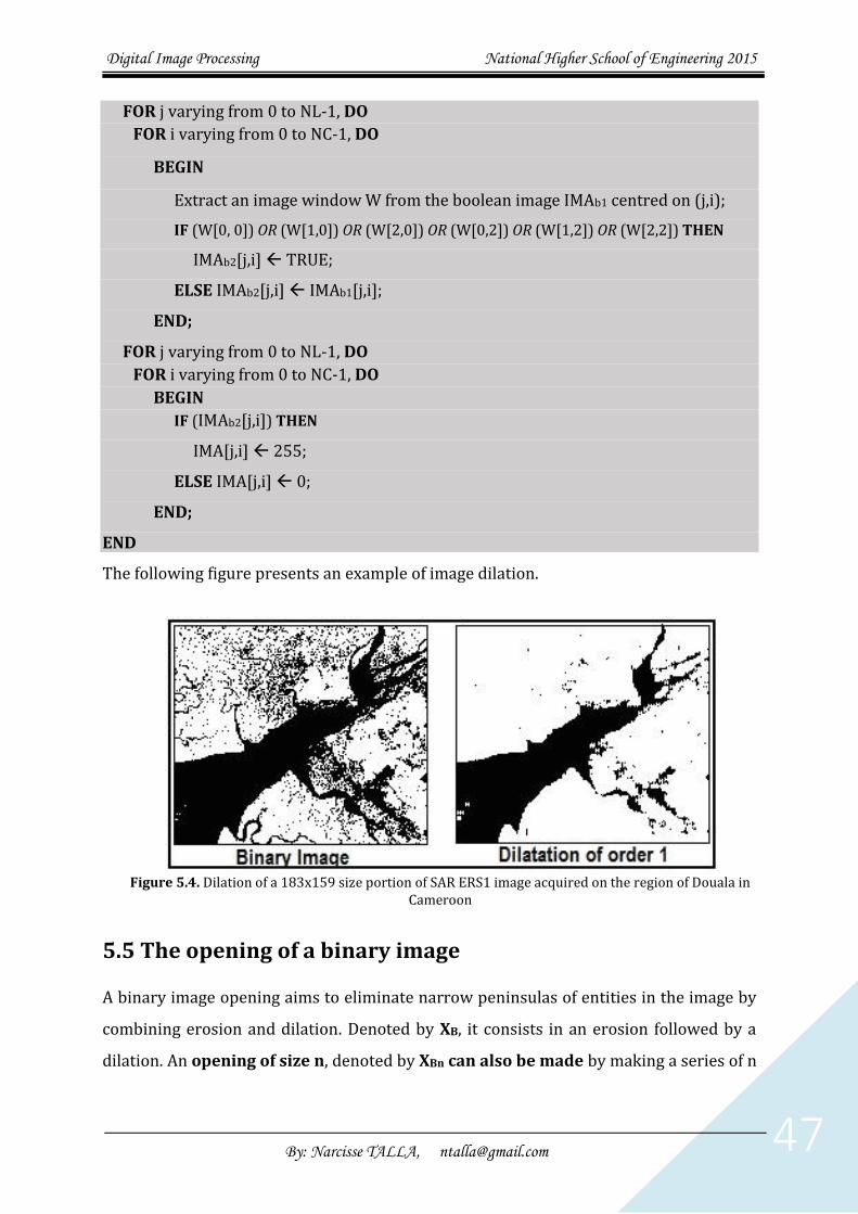
Digital Image Processing National Higher School of Engineering 2015
By: Narcisse TALLA, [email protected] 47
FOR j varying from 0 to NL-1, DO
FOR i varying from 0 to NC-1, DO
BEGIN
Extract an image window W from the boolean image IMAb1 centred on (j,i);
IF (W[0, 0]) OR (W[1,0]) OR (W[2,0]) OR (W[0,2]) OR (W[1,2]) OR (W[2,2]) THEN
IMAb2[j,i] TRUE;
ELSE IMAb2[j,i] IMAb1[j,i];
END;
FOR j varying from 0 to NL-1, DO
FOR i varying from 0 to NC-1, DO
BEGIN
IF (IMAb2[j,i]) THEN
IMA[j,i] 255;
ELSE IMA[j,i] 0;
END;
END
The following figure presents an example of image dilation.
Figure 5.4. Dilation of a 183x159 size portion of SAR ERS1 image acquired on the region of Douala in
Cameroon
5.5 The opening of a binary image
A binary image opening aims to eliminate narrow peninsulas of entities in the image by
combining erosion and dilation. Denoted by XB, it consists in an erosion followed by a
dilation. An opening of size n, denoted by XBn can also be made by making a series of n

Digital Image Processing National Higher School of Engineering 2015
By: Narcisse TALLA, [email protected] 48
erosions followed by a series of n dilations. The following image illustrates an opening of
an ERS-1 SAR image acquired on the region of Douala in Cameroon.
Figure 5.5. Opening of a 183x159 size portion of SAR ERS1 image acquired on the
region of Douala in Cameroon
5.6 The closure of a binary image
In contrary to the opening of a binary image, the closure of a binary image is an operation
that closes the bays and the small holes combining binary image erosion and dilation. The
binary image closure is the reverse of the opening. It consists in first applying a dilation
followed by an erosion. Obviously, a closure of size n (or of order n) denoted by XBn can be
realised by applying a series of n dilations followed by a series of n erosions. The following
figure presents an illustration of a binary image closure.
Figure 5.6. Closure of a portion of a SAR ERS-1 image of 183x159 size acquired on the
region of Douala in Cameroon
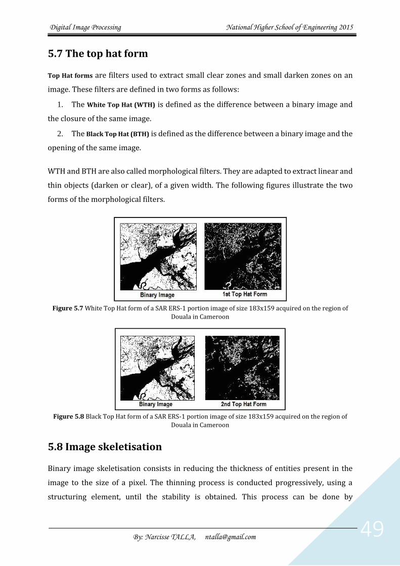
Digital Image Processing National Higher School of Engineering 2015
By: Narcisse TALLA, [email protected] 49
5.7 The top hat form
Top Hat forms are filters used to extract small clear zones and small darken zones on an
image. These filters are defined in two forms as follows:
1. The White Top Hat (WTH) is defined as the difference between a binary image and
the closure of the same image.
2. The Black Top Hat (BTH) is defined as the difference between a binary image and the
opening of the same image.
WTH and BTH are also called morphological filters. They are adapted to extract linear and
thin objects (darken or clear), of a given width. The following figures illustrate the two
forms of the morphological filters.
Figure 5.7 White Top Hat form of a SAR ERS-1 portion image of size 183x159 acquired on the region of
Douala in Cameroon
Figure 5.8 Black Top Hat form of a SAR ERS-1 portion image of size 183x159 acquired on the region of
Douala in Cameroon
5.8 Image skeletisation
Binary image skeletisation consists in reducing the thickness of entities present in the
image to the size of a pixel. The thinning process is conducted progressively, using a
structuring element, until the stability is obtained. This process can be done by

Digital Image Processing National Higher School of Engineering 2015
By: Narcisse TALLA, [email protected] 50
convoluting successively the image with the following 8 masks. Each mask Bj+1 is obtained
by the rotation of Bj of 45°.
B B B B1
0 0 0
0 1 0
1 1 1
2
0 0 0
1 1 0
1 1 0
3
1 0 0
1 1 0
1 0 0
4
1 1 0
1 1 0
0 0 0
B B B B5
1 1 1
0 1 0
0 0 0
6
0 1 1
0 1 1
0 0 0
7
0 0 1
0 1 1
0 0 1
8
0 0 0
0 1 1
0 1 1
The skeletisation algorithm is the following.
Algorithm 5.2 Image_Skeletisation
Input: IMG: Binary image to skeletise
NL, NC: respectively the number of lines and the number of columns of IMG;
Output: IMA: Skeleton image;
Local variables: i, j: integers
IMAb1, IMAb2: Array[0..NL-1; 0..NC-1] of Booleans;
BEGIN
FOR j varying from 0 to NL-1, DO
FOR i varying from 0 to NC-1, DO
BEGIN
IMAb2[i,j]FALSE;
IF (IMG[i,j]>0) THEN IMAb1[i,j]TRUE;
ELSE IMAb1[i,j]FALSE;
END;
Fill the borders of IMAb1 and IMAb2, using any of the three principles;
Iter 1;
Stable False;
WHILE (Stable=False) DO
BEGIN
StableTrue;
IterIter+1;
//Convolution with the East Mask
FOR j varying from 0 to NL-1, DO
FOR i varying from 0 to NC-1, DO

Digital Image Processing National Higher School of Engineering 2015
By: Narcisse TALLA, [email protected] 51
END
FalseStable
FalseijIMA
BEGIN
ELSE
ijIMAijIMA
THENijIMAANDijIMAANDijIMAAND
ijIMANOTORijIMAORijIMAORijIMAIF
b
bb
bbb
bbbb
;
;],[
],[],[
))]1,1[]1,[]1,1[
],[(]1,1[]1,[]1,1[
2
12
111
1111
//Convolution with the South-East Mask
FOR j varying from 0 to NL-1, DO
FOR i varying from 0 to NC-1, DO
END
FalseStable
FalseijIMA
BEGIN
ELSE
ijIMAijIMA
THENijIMAANDijIMAANDijIMAAND
ijIMANOTORijIMAORijIMAORijIMAIF
b
bb
bbb
bbbb
;
;],[
],[],[
))]1,1[],1[]1,[
],[(],1[]1,1[]1,[
1
21
222
2222
//Convolution with the South Mask
FOR j varying from 0 to NL-1, DO
FOR i varying from 0 to NC-1, DO
END
FalseStable
FalseijIMA
BEGIN
ELSE
ijIMAijIMA
THENijIMAANDijIMAANDijIMAAND
ijIMANOTORijIMAORijIMAORijIMAIF
b
bb
bbb
bbbb
;
;],[
],[],[
))]1,1[],1[]1,1[
],[(]1,1[],1[]1,1[
2
12
111
1111
//Convolution with the South-West Mask
FOR j varying from 0 to NL-1, DO
FOR i varying from 0 to NC-1, DO

Digital Image Processing National Higher School of Engineering 2015
By: Narcisse TALLA, [email protected] 52
END
FalseStable
FalseijIMA
BEGIN
ELSE
ijIMAijIMA
THENijIMAANDijIMAANDijIMAAND
ijIMANOTORijIMAORijIMAORijIMAIF
b
bb
bbb
bbbb
;
;],[
],[],[
))],1[]1,1[]1,[
],[(]1,[]1,[]1,1[
1
21
222
2222
//Convolution with the West Mask
FOR j varying from 0 to NL-1, DO
FOR i varying from 0 to NC-1, DO
END
FalseStable
FalseijIMA
BEGIN
ELSE
ijIMAijIMA
THENijIMAANDijIMAANDijIMAAND
ijIMANOTORijIMAORijIMAORijIMAIF
b
bb
bbb
bbbb
;
;],[
],[],[
))]1,1[]1,[]1,1[
],[(]1,1[]1,[]1,1[
2
12
111
1111
//Convolution with the North-West Mask
FOR j varying from 0 to NL-1, DO
FOR i varying from 0 to NC-1, DO
END
FalseStable
FalseijIMA
BEGIN
ELSE
ijIMAijIMA
THENijIMAANDijIMAANDijIMAAND
ijIMANOTORijIMAORijIMAORijIMAIF
b
bb
bbb
bbbb
;
;],[
],[],[
))]1,[]1,1[],1[
],[(],1[]1,1[]1,[
1
21
222
2222
//Convolution with the North Mask
FOR j varying from 0 to NL-1, DO
FOR i varying from 0 to NC-1, DO

Digital Image Processing National Higher School of Engineering 2015
By: Narcisse TALLA, [email protected] 53
END
FalseStable
FalseijIMA
BEGIN
ELSE
ijIMAijIMA
THENijIMAANDijIMAANDijIMAAND
ijIMANOTORijIMAORijIMAORijIMAIF
b
bb
bbb
bbbb
;
;],[
],[],[
))]1,1[],1[]1,1[
],[(]1,1[],1[]1,1[
2
12
111
1111
//Convolution with the North-East Mask
FOR j varying from 0 to NL-1, DO
FOR i varying from 0 to NC-1, DO
END
FalseStable
FalseijIMA
BEGIN
ELSE
ijIMAijIMA
THENijIMAANDijIMAANDijIMAAND
ijIMANOTORijIMAORijIMAORijIMAIF
b
bb
bbb
bbbb
;
;],[
],[],[
))]1,[]1,1[],1[
],[(],1[]1,1[]1,[
1
21
222
2222
END
FOR j varying from 0 to NL-1, DO
FOR i varying from 0 to NC-1, DO
IF (IMAb1[j,i]) THEN IMA[j,i]255;
ELSE IMA[j,i]0;
END
The following figure gives an example of skeletisation applied on the binary image of figure 5.2.
Figure 5.9 Skeletisation of a portion of a SAR image acquired by ERS-1 on the
Cameroonian Littoral region.

Digital Image Processing National Higher School of Engineering 2015
By: Narcisse TALLA, [email protected] 54
CHAPTER 6. TEXTURE ANALYSIS
6.1 Introduction
Distinct objects can have similar or identical spectral properties. This situation generally
generates confusions between thematic classes if the classification process is based only
on the spectral information contained in the image. This is why classification methods
based on spatial information have been developed, notably through texture analysis.
Texture analysis is a method that takes into account the spatial distribution of greyscales
in a given pixel neighbourhood in the image. Statistical methods are defined with respect
to various orders.
6.2 First order statistical methods
6.2.1. Definition
First order statistical methods are based on first order histograms. Such a histogram
specifies the frequency of appearance of a given greyscale in a given neighbourhood of the
image called image window. An image window is a rectangular or square portion of the
image. From the histogram, one can extract various statistical parameters. The following
section illustrates some of them.
6.2.2 Examples of first order statistical parameters
Let consider an image window W of size Wx colums and Wy lines. The probability P(i) of
occurrence of the greyscale i in W is given by WW yx
iNiP
*)(
)( , where N(i) is the
number of greyscales i in W. Let denote by MaxGs the maximum greyscale in W. The
following equations define some statistical parameters of order 1.
Average or Mean:
MaxGs
i
M iPiS0
)( (Eq. 6.1)
This parameter represents the location of the histogram on the scale of pixel greyscales.
Entropy:
MaxGs
i
iPLogiPEnt0
2 )()( (Eq. 6.2)
This parameter measures the image complexity. In other words, it measures the degree
of disorder in the image.

Digital Image Processing National Higher School of Engineering 2015
By: Narcisse TALLA, [email protected] 55
Standard Deviation:
MaxGs
i
D MS Si
0
2 (Eq. 6.3)
This parameter measures the organisation of greyscales around the Average.
Skewness:
MaxGs
i
iPM
D
Skw SiS 0
3
3)(
1 (Eq. 6.4)
This parameter measures the histogram dissimilarity. i.e. if it is well equilibrated around
the Average or if it is left or right oriented with respect to the mean.
Kurtosis:
MaxGs
i
iPM
D
Kurt SiS 0
4
4)(
1 (Eq. 6.5)
This parameter gives an indication on the histogram aspect. i.e. if it is flatten or not.
6.2.3. Illustration
Let calculate for example the parameter Mean for the following simple digital image IMG
specified on the left of the following figure. Let calculate the values of P(i) for all the
greyscales of the image, using a 3x3 size image window and the symmetry principle of
border filling.
Figure 6.1. Original image and border filled image with the principle of symmetry.
From the first pixel IMG00 (greyscale 205), the following image window is extracted.
W205
174 215 174
242 205 242
174 215 174
We have: Wx=Wy=3;
P(174) = N(174)/(3*3) = 4/9; P(215) = N(215)/M = 2/9;
P(242) = N(242)/(3*3) = 2/9; P(205) = N(205)/M = 1/9;
The value of the parameter Mean related to the greyscale 205 is given by:
SM(205) = ENT[(174x4/9)+(215x2/9)+(242x2/9)+(205x1/9)] = ENT[201.66] = 201
Where ENT is the entire part function.

Digital Image Processing National Higher School of Engineering 2015
By: Narcisse TALLA, [email protected] 56
The process is repeated with the same principle to other pixels of the original image IMG
and, considering that Wij is an image window of size 3*3 centred on the pixel (i,j) of IMG,
we obtain the following results:
SM(W01) = 192; SM(W02) = 187; SM(W10) = 181; SM(W11) = 183;
SM(W12) = 172 ; SM(W20); = 165 SM(W21) = 184; SM(W22) = 170.
The following figure presents the image texture of the parameter Mean obtained.
Figure 6.2. Example of image texture: The parameter Mean
6.3 Second order statistical methods
6.3.1 Definition
These methods are based on the second order histograms called co-occurrence matrices.
The co-occurrence matrix expresses the probability of appearance of each couple of
greyscales (i,j) in the image window, with respect to a given direction and inter-pixels
distance. Below are some commonly used order-2 texture parameters.
Energy or second angular moment:
MaxGs
i
MaxGs
j
djiPE0 0
2),,,( (Eq. 6.6)
The energy parameter measures the homogeneity of the image. Its value is low when the
values of the co-occurrence matrix are nearer. In contrary, if some values of the co-
occurrence matrix are very bigger than others, the value of the energy becomes high.
Entropy:
MaxGs
i
MaxGs
j
djiPdjiPEnt0 0
2 )),,,((log),,,( (Eq. 6.7)
The entropy is great when the values of the co-occurrence matrix are almost equal each
to another. Otherwise, its value is low.
Contrast or inertia:
MaxGs
i
MaxGs
j
djiPCont ji0 0
2
),,,( (Eq. 6.8)
The inertia parameter measures the contrast (or the local variation of greyscales) in the
image. Its value is great when the values of the co-occurrence matrix are concentrated far
from the diagonal. If in contrary the values of the co-occurrence matrix are concentrated
around the diagonal then the contrast is weak.

Digital Image Processing National Higher School of Engineering 2015
By: Narcisse TALLA, [email protected] 57
Correlation: yx
MaxGs
i
MaxGs
j
yx djiPjiCorr /),,,())((0 0
(Eq. 6.9)
The correlation has a great value when the values of the co-occurrence matrix are
uniformly distributed. Otherwise, its value is low.
Cluster prominence:
MaxGs
i
MaxGs
j
djiPyxCpr ji0 0
4
),,,()( (Eq. 6.10)
Where:
P i j d( , , , ) is the probability of appearance of the couple of greyscales (i,j) in the
direction Ɵ, with an inter-pixels distance d.
x
and x
represent respectively the mean and the standard deviation with
respect to the lines of the co-occurrence matrix.
y
and y
represent respectively the mean and the standard deviation with
respect to the columns of the co-occurrence matrix.
6.3.2 Co-occurrence matrix
The co-occurrence matrix is defined with respect to a given direction. In what follows,
algorithms of the co-occurrence matrix for the four principal directions, notably 0°, 45°,
90° and 135° are presented.

Digital Image Processing National Higher School of Engineering 2015
By: Narcisse TALLA, [email protected] 58
Algorithm 6.1. CooccurrenceMatrix_0°_Direction Input: W: Image window of size Wx columns and Wy lines; MaxGs: Maximum greyscale in the image; d: inter-pixel distance; Output: CM: Co-occurrence matrix of size (MaxGs+1)*(MaxGs+1); Local Variables: i, j, x, y: Integers; Begin For j varying from 0 to MaxGs do For i varying de 0 to MaxGs do CM[j,i] 0 ; //Initialisation For y varying from 0 to Wy-1 do For x varying from 0 to Wx-1-d do Begin I W[y,x] J W[y,x+d] CM [I,J] CM [I,J] + 1; CM [I,J] CM [J,I] + 1; End For j varying from 0 to MaxGs do For i varying from 0 to MaxGs do MC [i,j] MC [j,i]/(Wy*(Wx-d)); End
Algorithm 6.2. CooccurrenceMatrix_45°_Direction Input: W: Image window of size Wx columns and Wy lines; MaxGs: Maximum greyscale in the image; d: inter-pixel distance; Output: CM: Co-occurrence matrix of size (MaxGs+1)*(MaxGs+1); Local Variables: i, j, x, y: Integers; Begin For j varying from 0 to MaxGs do For i varying de 0 to MaxGs do CM[j,i] 0 ; //Initialisation For y varying from 0 to Wy-1-d do For x varying from 0 to Wx-1-d do Begin I W[y,x] J W[y+d,x+d] CM [I,J] CM [I,J] + 1; CM [I,J] CM [J,I] + 1; End For j varying from 0 to MaxGs do For i varying from 0 to MaxGs do MC [i,j] MC [j,i]/((Wy-d)*(Wy-d)); End

Digital Image Processing National Higher School of Engineering 2015
By: Narcisse TALLA, [email protected] 59
Algorithm 6.3. CooccurrenceMatrix_90°_Direction Input: W: Image window of size Wx columns and Wy lines; MaxGs: Maximum greyscale in the image; d: inter-pixel distance; Output: CM: Co-occurrence matrix of size (MaxGs+1)*(MaxGs+1); Local Variables: i, j, x, y: Integers; Begin For j varying from 0 to MaxGs do For i varying de 0 to MaxGs do CM[j,i] 0 ; //Initialisation For y varying from d to Wy-1 do For x varying from 0 to Wx-1 do Begin I W[y,x] J W[y-d,x] CM [I,J] CM [I,J] + 1; CM [I,J] CM [J,I] + 1; End For j varying from 0 to MaxGs do For i varying de 0 to MaxGs do MC [i,j] MC [j,i]/(Wx*(Wy-d)); End
Algorithm 6.4. CooccurrenceMatrix_135°_Direction Input: W: Image window of size Wx columns and Wy lines; MaxGs: Maximum greyscale in the image; d: inter-pixel distance; Output: CM: Co-occurrence matrix of size (MaxGs+1)*(MaxGs+1); Local Variables: i, j, x, y: Integers; Begin For j varying from 0 to MaxGs do For i varying de 0 to MaxGs do CM[j,i] 0 ; //Initialisation For y varying from d to Wy-1 do For x varying from d to Wx-1 do Begin I W[y,x] J W[y-d,x-d] CM [I,J] CM [I,J] + 1; CM [I,J] CM [J,I] + 1; End For j varying from 0 to MaxGs do For i varying from 0 to MaxGs do MC [i,j] MC [j,i]/((Wy-d)*(Wx-d)); End

Digital Image Processing National Higher School of Engineering 2015
By: Narcisse TALLA, [email protected] 60
6.3.3 Image texture
In this section, we apply directly the principle on an example. Let consider for example
the parameter Energy. The following algorithm specifies the technique of Energy image
texture construction.
Algorithm 6.5 Energy_Image_Texture
Input: IMG: Original image of size NL lines and NC columns;
MaxGs: maximum greyscale in IMG;
Ɵ, d: respectively the direction and the inter-pixel distance;
Output: ENR_IMG: Energy texture image with the same size as IMG;
Local Variables: x,y,i,j: integers;
IMA: Array[0..NL-1; 0..NC-1] of reals;
E, E_Max: reals;
BEGIN
FOR y varying from 0 to NL-1 DO
FOR x varying from 0 to NC-1 DO
Begin
1- Extract an image window of size Wx columns and Wy lines centred on the
pixel (y,x) of IMG;
2- Calculate the co-occurrence matrix CM related to W, in the direction Ɵ and
the inter-pixel distance d;
3- E 0; E_Max 0;
4- FOR j varying from 0 to MaxGs DO
FOR i varying from 0 to MaxGs DO
E E+(CM[j,i]*CM[j,i]);
5- IMA[y,x] E;
6- IF (E > E_max) THEN E_max E;
End
FOR y varying from 0 to NL-1 DO
FOR x varying from 0 to NC-1 DO
ENR_IMG[y,x] ENT((255* IMA[y,x])/E_max);
END
ENT is the entire part function.
It is also possible to consider all the directions at once, either by taking the average value
of the co-occurrence matrices in various directions, or by taking the maximum value of
the co-occurrence matrix.

Digital Image Processing National Higher School of Engineering 2015
By: Narcisse TALLA, [email protected] 61
6.3 Grayscale ranges lengths method
The method of grayscale ranges lengths considers an auto-adaptive and mono-
dimensional neighbourhood. A point belongs to a neighbourhood of the current point if
its greyscale is less different. The size of the neighbourhood is then variable and
constitutes a major characteristic parameter in this approach. The grayscale ranges length
method consists in counting, in the image, the number of ranges of greyscales of a given
length, in a given direction. A matrix R( ) of grayscale ranges lengths is associated to a
direction of angle . From this matrix, the following parameters can be extracted.
Short Run Low Greyscale Emphasis
M
i
N
j ji
jir
nrSRLGE
1 122
);,(1 (Eq. 6.11)
Short Run High Greyscale Emphasis
M
i
N
j j
jiri
nrSRHGE
1 12
2 );,(1 (Eq. 6.12)
Long Run Low Greyscale Emphasis
M
i
N
j i
jirj
nrLRLGE
1 12
2 );,(1 (Eq. 6.13)
Long Run High Greyscale Emphasis
M
i
N
j
jirjinr
LRHGE1 1
22 );,(1
(Eq. 6.14)
Distribution of greyscales 2
1 1
;,1
M
i
N
j
jirnr
DGS (Eq. 6.15)
Distribution of lengths of ranges 2
1 1
;,1
N
j
M
i
jirnr
DLR (Eq. 6.16)
Greyscales Percentage
M
i
N
j
jirNB
GSP1 1
;,1
(Eq. 6.17)
Low greyscale range
M
i
N
j i
jir
nrLSGSR
1 12
;,1 (Eq. 6.18)
High greyscale range
M
i
N
j
jirinr
HGR1 1
2 ;,1
(Eq. 6.19)
The constant
M
i
N
j
jirnr1 1
);,( is the total number of ranges in the image window, with
respect to the orientation Ɵ, centred on the current pixel. M and N are respectively the
number of greyscales and ranges in the image window. r[] is the matrix of wavelength
ranges in a given direction. Its specification with respect to the four principal directions
is the following.
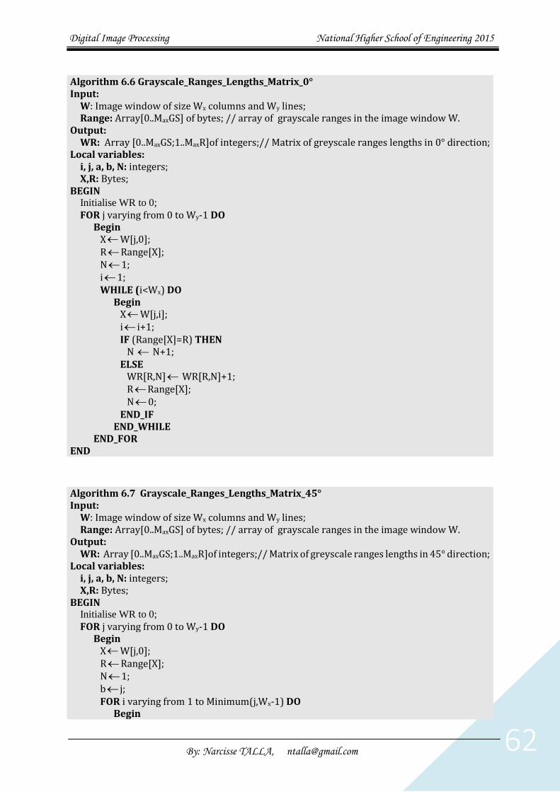
Digital Image Processing National Higher School of Engineering 2015
By: Narcisse TALLA, [email protected] 62
Algorithm 6.6 Grayscale_Ranges_Lengths_Matrix_0° Input:
W: Image window of size Wx columns and Wy lines; Range: Array[0..MaxGS] of bytes; // array of grayscale ranges in the image window W.
Output: WR: Array [0..MaxGS;1..MaxR]of integers;// Matrix of greyscale ranges lengths in 0° direction;
Local variables: i, j, a, b, N: integers; X,R: Bytes;
BEGIN Initialise WR to 0;
FOR j varying from 0 to Wy-1 DO Begin
XW[j,0]; RRange[X]; N1; i1; WHILE (i<Wx) DO
Begin XW[j,i]; i i+1; IF (Range[X]=R) THEN
N N+1; ELSE
WR[R,N] WR[R,N]+1; RRange[X]; N0;
END_IF END_WHILE
END_FOR END
Algorithm 6.7 Grayscale_Ranges_Lengths_Matrix_45° Input:
W: Image window of size Wx columns and Wy lines; Range: Array[0..MaxGS] of bytes; // array of grayscale ranges in the image window W.
Output: WR: Array [0..MaxGS;1..MaxR]of integers;// Matrix of greyscale ranges lengths in 45° direction;
Local variables: i, j, a, b, N: integers; X,R: Bytes;
BEGIN Initialise WR to 0;
FOR j varying from 0 to Wy-1 DO Begin
XW[j,0]; RRange[X]; N1; b j; FOR i varying from 1 to Minimum(j,Wx-1) DO
Begin

Digital Image Processing National Higher School of Engineering 2015
By: Narcisse TALLA, [email protected] 63
XW[b-1,i]; bb-1; IF (Range[X]=R) THEN
N N+1; ELSE
Begin WR[R,N] WR[R,N]+1; RRange[X]; N0;
END_IF END_FOR
END_FOR FOR i varying from 1 to Wx-1 DO
Begin XW[Wy-1,i]; RRange[X]; N1; bWy-1; FOR a varying from 0 to Minimum(Wy-1,i) DO
Begin XW[b-1,a]; bb-1; IF (Range[X]=R) THEN
N N+1; ELSE
Begin WR[R,N] WR[R,N]+1; RRange[X]; N0;
END_IF END_FOR
END_FOR END

Digital Image Processing National Higher School of Engineering 2015
By: Narcisse TALLA, [email protected] 64
Algorithm 6.8 Grayscale_Ranges_Lengths_Matrix_90° Input:
W: Image window of size Wx columns and Wy lines; Range: Array[0..MaxGS] of bytes; // array of grayscale ranges in the image window W.
Output: WR: Array [0..MaxGS;1..MaxR]of integers;// Matrix of greyscale ranges lengths in 90° direction;
Local variables: i, j, a, b, N: integers; X,R: Bytes;
BEGIN Initialise WR to 0;
FOR i varying from 0 to Wx-1 DO Begin
XW[0,i]; RRange[X]; N1; j1; WHILE (j<Wy) DO
Begin XW[j,i]; j j+1; IF (Range[X]=R) THEN
N N+1; ELSE
WR[R,N] WR[R,N]+1; RRange[X]; N0;
END_IF END_WHILE
END_FOR END
Algorithm 6.9 Grayscale_Ranges_Lengths_Matrix_135° Input:
W: Image window of size Wx columns and Wy lines; Range: Array[0..MaxGS] of bytes; // array of grayscale ranges in the image window W.
Output: WR: Array [0..MaxGS;1..MaxR]of integers;// Matrix of greyscale ranges lengths in 135°
direction; Local variables:
i, j,a,b, N: integers; X,R: Bytes;
BEGIN Initialise WR to 0;
FOR j varying from 0 to Wy-1 DO Begin
XW[j,Wx-1]; RRange[X]; N1; b j; FOR i varying from 1 to Minimum(j,Wx-1) DO
Begin

Digital Image Processing National Higher School of Engineering 2015
By: Narcisse TALLA, [email protected] 65
Where:
MaxGS is the maximum greyscale in the image window W;
MaxR is the maximum length of a range in the image window. It is defined as
follows:
o MaxR=NL if direction=90°;
o MaxR=NC if direction=0°;
o MaxR=Minimum(NL;NC) otherwise.
Sometime, it is important to resample the image for the execution time optimisation
purpose. Image resampling consists in reducing uniformly the values of the greyscales
present in the image. Following is the related algorithm.
XW[b-1, Wx-1-i]; bb-1; IF (Range[X]=R) THEN
N N+1; ELSE
Begin WR[R,N] WR[R,N]+1; RRange[X]; N0;
END_IF END_FOR
END_FOR FOR i varying from Wx-2 down to 0 DO
Begin XW[Wy-1,i]; RRange[X]; N1; bWy-1; FOR a varying from 1 to Minimum(Wy-1,i) DO
Begin XW[b-1, i-a]; bb-1; IF (Range[X]=R) THEN
N N+1; ELSE
Begin WR[R,N] WR[R,N]+1; RRange[X]; N0;
END_IF END_FOR
END_FOR END
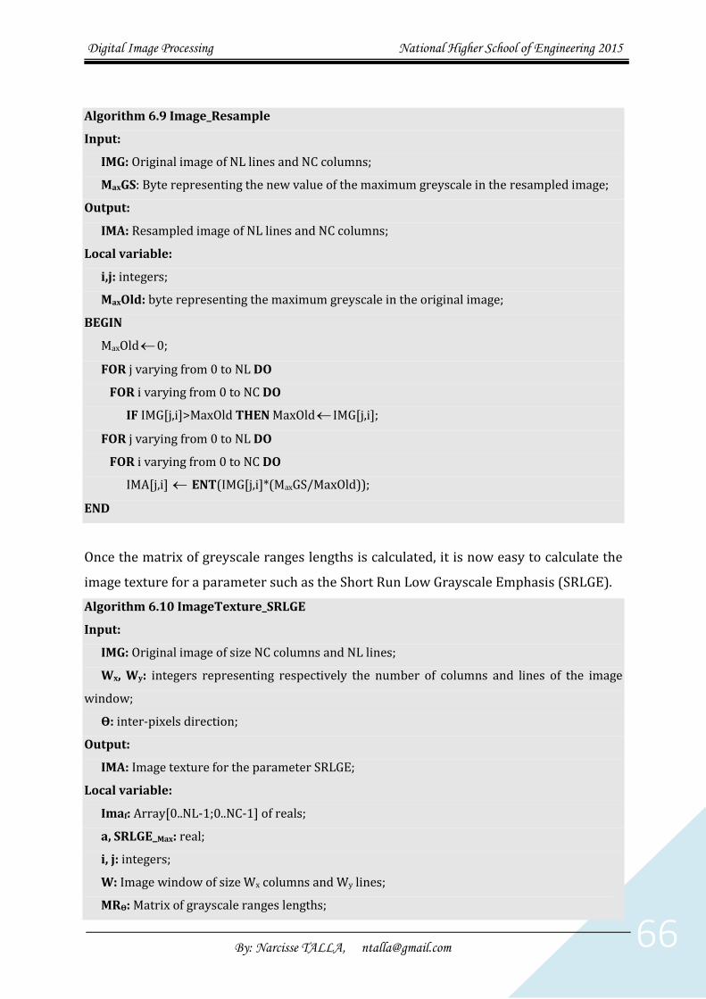
Digital Image Processing National Higher School of Engineering 2015
By: Narcisse TALLA, [email protected] 66
Algorithm 6.9 Image_Resample
Input:
IMG: Original image of NL lines and NC columns;
MaxGS: Byte representing the new value of the maximum greyscale in the resampled image;
Output:
IMA: Resampled image of NL lines and NC columns;
Local variable:
i,j: integers;
MaxOld: byte representing the maximum greyscale in the original image;
BEGIN
MaxOld0;
FOR j varying from 0 to NL DO
FOR i varying from 0 to NC DO
IF IMG[j,i]>MaxOld THEN MaxOldIMG[j,i];
FOR j varying from 0 to NL DO
FOR i varying from 0 to NC DO
IMA[j,i] ENT(IMG[j,i]*(MaxGS/MaxOld));
END
Once the matrix of greyscale ranges lengths is calculated, it is now easy to calculate the
image texture for a parameter such as the Short Run Low Grayscale Emphasis (SRLGE).
Algorithm 6.10 ImageTexture_SRLGE
Input:
IMG: Original image of size NC columns and NL lines;
Wx, Wy: integers representing respectively the number of columns and lines of the image
window;
Ɵ: inter-pixels direction;
Output:
IMA: Image texture for the parameter SRLGE;
Local variable:
Imaf: Array[0..NL-1;0..NC-1] of reals;
a, SRLGE_Max: real;
i, j: integers;
W: Image window of size Wx columns and Wy lines;
MRƟ: Matrix of grayscale ranges lengths;

Digital Image Processing National Higher School of Engineering 2015
By: Narcisse TALLA, [email protected] 67
NR: integer representing number of ranges of grayscales in the image window W;
BEGIN
SRLGE_Max0;
FOR y varying from 0 to NL-1 DO
FOR x varying from 0 to NC-1 DO
Begin
Extract and image window W centred on the pixel (y,x) of the image IMG;
Calculate the matrix MRƟ of wavelength ranges of greyscales related to W in the direction Ɵ;
a0;
FOR i varying from 0 to MaxGS, DO
FOR j varying from 1 to NR DO
aa+(MRƟ(i, j)/[(i+1)² (j+1)²]);
aa/NR;
Imaf[y,x]a;
IF(a > SRLGE_Max) THEN SRLGE_Max a;
End
FOR y varying from 0 to NL-1 DO
FOR x varying from 0 to NC-1 DO
Begin
Imaf[y,x]ENT((255* imaf[x,y])/SRLGE_Max);
END
Where ENT is the entire part function.

Digital Image Processing National Higher School of Engineering 2015
By: Narcisse TALLA, [email protected] 68
CHAPTER 7. IMAGE CLASSIFICATION
7.1 Introduction
Remote sensing data can be analysed for the extraction of useful thematic information.
The multispectral classification is one of the most used for information retrieval. This
technique supposes that images of a given geographical region are distributed in different
electromagnetic spectrum. A multispectral classification can be done by the means of
various algorithms among which:
Supervised statistical or neuronal classification methods;
Unsupervised statistical or neuronal classification methods;
Fuzzy classification methods
Expert systems or knowledge-based classification methods.
Hybrid methods based on the previous methods.
The supervised classification method supposes that the analyst has some knowledge of
the field from which the image was acquired. This knowledge obtained through field
mission or validated maps of the area of study helps to identify training sites on the image.
These training sites are used to train the classifier before the automation of the process.
Each training site characterises an information or thematic class such as, Lake, Forest,
Road, Crops, etc.
In contrary to the supervised methods, the unsupervised (non-supervised) method
supposes that the analyst doesn’t have any knowledge of the area. i.e no field mission has
been conducted on the area of study and there is no available map of the region of study.
The analyst just specifies the number of spectral classes and the classifier, based on
spectral information, tries its best to classify the image. These spectral classes are
interpreted by the analyst to produce information classes.
The fuzzy classification method considers the heterogeneous and inaccurate nature of
geographical data. It can be either based on supervised or non-supervised algorithms.
Most of classification algorithms use Boolean theory of sets to produce homogeneous
information classes, completely ignoring the inaccuracy nature of geographical data.
Instead of assigning each pixel of the image to a unique class among M others, the fuzzy
classification calculates M real numbers indicating the degree of nearness of the pixel to

Digital Image Processing National Higher School of Engineering 2015
By: Narcisse TALLA, [email protected] 69
each class of interest. This information is afterwards used by the analyst to extract more
accurate information on the area of study such as the heterogeneous pixels composition.
Sometimes, it is necessary to include auxiliary and non-spectral data in a fuzzy supervised
or unsupervised classification to extract expected information. Among such methods, one
can distinguish hierarchical, expert systems and knowledge-based classifications.
7.2 Classification process
7.2.1 Classification protocol
A good classification (supervised or non-supervised) of remote sensing data is tributary
to the mastering of the following steps:
1) Identification and selection of a region of interest (ROI) on which hypothesis
should be tested. The classes of interest to be tested in the hypothesis determine the
nature of the classification method to use.
2) Selection of the appropriate remote sensing images, considering environmental
and data acquisition system constraints. Based on these constraints, radiometric and/or
geometric corrections are done on images finally acquired.
3) Choice of the appropriate classification algorithm and collection of initial training
data.
4) Identification of statistical parameters that better discriminate the training data.
5) Training of the classifier with the parameters selected in the previous step, in case
of a supervised classification.
6) Collection of additive training data for the evaluation of the classifier
performances. If the performances are acceptable, the classifier is adopted for the global
image classification.
7) Evaluation of the classification error. If the result is satisfactory then the
classification maps are validated.
7.2.2 Classification system
There is a great difference between an information class present on the field and a spectral
class contained in an image. Information classes are categories of interest for data users,
such as geological, forest and crops units that give information to the manager,
administrators and scientists in charge of remote sensing data.

Digital Image Processing National Higher School of Engineering 2015
By: Narcisse TALLA, [email protected] 70
Spectral classes are groups of pixels that have similar spectral characteristics directly
observable on the image. An image becomes a good source of information when there is a
link between spectral classes observable on the image and information classes present on
the field. Thus, remote sensing classification consists in establishing a correspondence
between spectral and information classes. When this correspondence is accurate, the
resulting classification maps are reliable. Otherwise, the image is not a good source of
information.
In the same information class, spectral characteristics can vary, due to the natural
environment. For example, in a Forest information class, spectral characteristics can
change with the type and age of trees. So the same information class can contain many
spectral classes. Similarly, two or more different information classes can have the same
spectral information. For example, under a certain wavelength, the spectral information
of the Lake is similar to the spectral information of a targeted road.
7.2.3 Training sites selection and statistics extraction
Training sites in remote sensing must be representative of land cover, after the
classification system is adopted. The quality of training data depends on the homogeneity
of the environment. If the land characteristics varies along the region of study then the
spectral properties of the training data collected should not be homogeneous, generating
the problem of spectral signatures extension. In this case, following are some factors that
help to solve the problem:
Differences on soil types;
Water turbidity;
Types of crops;
Unusual soil humidity conditions, eventually caused by non-uniform
precipitations;
diffuser plates of atmospheric gases;
Once extension factors of spectral signatures are considered, training sites are selected
and characterised for each information class. In case of n spectral bands (multiband
image), each pixel of the training site is represented by an array Xc of measures defined
by the following equation.

Digital Image Processing National Higher School of Engineering 2015
By: Narcisse TALLA, [email protected] 71
GV
GV
X
m
ij
m
ij
m
c
1
1
(Eq. 6.1)
Where GVm
ij1
is the grayscale of the mth pixel at location (i,j) in band k. Combining all the N
pixels of the training site of an information class, the characteristic vector Mc of the
information class is the following.
Mc
c
cn
1
(Eq. 6.2)
Where ck is the average value of the characteristic vectors of the N training pixels
selected in the class Ck. These characteristic vectors can also be analysed to provide the
following characteristic covariance matrix:
V
Cov Cov
Cov Cov
c
cll cnl
cnl cnn
(Eq. 6.3)
Where Covckl is the covariance of class C between bands k and l.
7.2.4 Reduction of parameters
The representation of input data of a static or neuronal classification system is very
important. It can significantly affect the performances of the system. There are two
approaches of parameters reduction: parameters extraction and parameters selection.
Parameters extraction is an operation that consists in finding a set of vectors representing
the observation by reducing the dimensionality. Despite the fact that the reduction of the
dimensionality is useful, the inducted error must not scarify the discrimination power of
the classifier. Methods of parameters extraction can be supervised or non-supervised,
linear or non-linear. Among these methods, one can distinguish the principal components
analysis. For all these methods, a characteristic matrix is defined. From this matrix,
eigenvalues and corresponding eigenvectors are calculated and decreasingly ordered.
The dimension of the input data corresponds to the number of eigenvectors selected.

Digital Image Processing National Higher School of Engineering 2015
By: Narcisse TALLA, [email protected] 72
Transformed data are determined by Y XT , where is the transformation matrix
made of eigenvectors of the characteristic matrices, X is the input data vector in the
original characteristic space and Y is the output data vector in the new characteristic
space.
7.3 Supervised image classification algorithms
A supervised image classification algorithm consists in three steps:
1) Training step: For each information class identified in the image, a certain
number of pixels are selected and characterised with the perspective of training
the classifier.
2) Information Classes allocation step: Each pixel of the pixel is assigned to
information class with which the likelihood is maximum.
3) Verification step: The quality of classification s evaluated.
Following are some commonly used supervised classification algorithms:
Parallelepiped decision rule;
Minimal distance decision rule;
k nearest neighbours decision rule;
Maximum likelihood decision rule.
To these methods, one must add classification methods based on artificial neuronal
networks.
7.3.1 Parallelepiped method for image classification
This Boolean logic method-based method is widely used. Training data in n spectral bands
are used in the classification process. For each information class C, the characteristic
vector Vc is calculated.
cn
c
cV
1
Where ck represents the average greyscale of selected
pixels in the information class C in bad k. Let ck be the standard deviation of training
data of the information class C in band k. Considering ck as the classification threshold
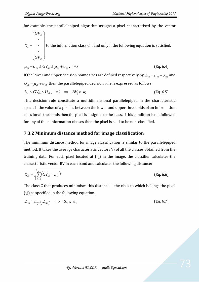
Digital Image Processing National Higher School of Engineering 2015
By: Narcisse TALLA, [email protected] 73
for example, the parallelepiped algorithm assigns a pixel characterised by the vector
ijn
ij
c
GV
GV
X
1
to the information class C if and only if the following equation is satisfied.
kGV ckckijkckck , (Eq. 6.4)
If the lower and upper decision boundaries are defined respectively by ckckckL and
ckckckU then the parallelepiped decision rule is expressed as follows:
cijckijkck wBVkUGVL , (Eq. 6.5)
This decision rule constitute a multidimensional parallelepiped in the characteristic
space. If the value of a pixel is between the lower and upper thresholds of an information
class for all the bands then the pixel is assigned to the class. If this condition is not followed
for any of the n information classes then the pixel is said to be non-classified.
7.3.2 Minimum distance method for image classification
The minimum distance method for image classification is similar to the parallelepiped
method. It takes the average characteristic vectors Vc of all the classes obtained from the
training data. For each pixel located at (i,j) in the image, the classifier calculates the
characteristic vector BV in each band and calculates the following distance:
n
k
ckijkcij GVD1
2 (Eq. 6.6)
The class C that produces minimises this distance is the class to which belongs the pixel
(i,j) as specified in the following equation.
D D X wcijk
kij ij c min (Eq. 6.7)

Digital Image Processing National Higher School of Engineering 2015
By: Narcisse TALLA, [email protected] 74
Figure 7.1. Example of a minimum distance image classification applied on a SPOT image acquired on the Yaounde town.
7.3.3 K nearest neighbours method for image classification
As the previous method, the K nearest neighbours method is based on the characteristic
vectors aXna1
of the training pixels, N being the number of training pixels in the
information class X. The classifier calculates the Euclidian distance between the
characteristic vector ijkGVnk1
of each unknown pixel (i,j) and each characteristic vector
Xi of the training pixel i, n being the number of bands. The process end by determining
appearance frequency fck of pixels of each class C between the K nearest pixels of the
considered pixel. The following equation formalises the process.
kijckc
ck wGVff max (Eq. 6.8)
It is obviously required that K should be defined. Practically, The value of K is given by
NcK , where c is an appropriate constant (typically, c=1) and N is the total number of
training pixels. When K=1, this decision rule corresponds to the method of minimum
distance.
7.3.4 Maximum likelihood method for digital image classification
The maximum likelihood decision rule assigns each pixel of characteristic vector X to the
information class C for which the components are more capable of producing the
characteristic vector X. The maximum likelihood method for image classification uses the
statistics calculated on each class, including the Mean c and the covariance matrix Vc for
each class C. This decision rule assigns the vector X to the class C if and only if the following
equations are satisfied.

Digital Image Processing National Higher School of Engineering 2015
By: Narcisse TALLA, [email protected] 75
p X p X X wcj
j c max (Eq. 6.9)
p XV
X V Xc n
c
c
T
c c
1
2
1
22 1 2
1
exp (Eq. 10)
Where Vc represents the Determinant of the covariance matrix Vc .
To assign a characteristic vector X of an unknown pixel to an information class, the
classifier calculates the value of p Xc for each class. The pixel belongs to the class that
maximises this value. The following figure presents an example of a multispectral image
classification using the maximum likelihood method.
Figure 7.2. Example of Yaoundé town SPOT image classification using the maximum likelihood method.
7.4 Non-supervised classification algorithms
In contrary to supervised classification, the non-supervised classification requires only a
minimal quantity of initial inputs. Numerical operations are done to determine natural
groupings of spectral properties of pixels in the space of multispectral characteristics.
The classifier calculates the segments’ statistics (Mean and covariance matrix) to use for
the classification. Once data are classified, the analyst tries to assign these natural or
spectral classes to information classes. This task is not ease at all because some segments
doesn’t have any signification on the field, for example a mixture of different information
classes. It is therefore absolutely necessary to better understand the spectral
characteristics on the field, to be able to consider certain segments as representing
information classes. Various methods of image segmentation have been developed for

Digital Image Processing National Higher School of Engineering 2015
By: Narcisse TALLA, [email protected] 76
multiple applications starting from Pattern Recognition to remote sensing. Segmentation
algorithms used for non-supervised classification of remote sensing images don’t
generally have the same efficiency. This is why various approaches were progressively
developed.
7.4.1 Histogram modes method for image classification
A mono-dimensional histogram of an image is a graphical representation of greyscales’
frequencies. It is a two-dimensional graph with grayscales on abscises and frequencies on
ordinates. A histogram mode is a local maximum, while a histogram valley is a local
minimum of the histogram. A histogram mode indicates a grouping of pixels and helps to
detect spectral classes. The greyscale corresponding to a maximum in the histogram is a
centre of the spectral class. Following is an algorithm of image classification based on a
mono-dimensional histogram.
Algorithm 7.1 Image_Classification_By_Histogram
Input: IMG: unclassified digital image of size NC columns and NL lines;
Output: IMA: classified digital image with the same size as IMG;
Local variable:
K,i,j,n=0: integer;
H: Array[0,..,GSMax] of integers;// GSMax is the maximum greyscale in the image;
C: Array[0,..,N] of bytes; // Array of centres of spectral classes;
BEGIN
Determine the maximum greyscale GSMax and the number N of classes of the image IMG;
FOR i varying from 0 to GSMax DO
H[i]0; //Initialisation of the Histogram;
FOR j varying from 0 to NL DO
FOR i varying from 0 to NC DO
H(IMG[j,i]) IMG[j,i]+1; //Construction of the histogram;
FOR i varying from 1 to GSMax-1 DO
IF(H[i-1]<H[i]>H[i+1]) THEN
C[n]I;
nn+1;
END_IF
FOR j varying from 0 to NL DO

Digital Image Processing National Higher School of Engineering 2015
By: Narcisse TALLA, [email protected] 77
FOR i varying from 0 to NC DO
BEGIN
x IMG[j,i];
aC[0];
FOR k varying from 1 to N DO
IF (C[k]-x)<(a-x) THEN
aC[k];
END_FOR
IMA[j,i]a;
END_FOR
END
The following figure illustrates the algorithm. The original image is acquire on the
Cameroonian Atlantic coast.
Figure 7.3 Classification of an ESAR image using the histogram mode method.
A multi-band classification can also be done by the means of a bi-dimensional histogram.
Such histogram counts the number of occurrences of each pair of greyscales of equivalent
pixels in the two bands. Once the bi-dimensional histogram is calculated, the classification
algorithm is similar to the previous one.

Digital Image Processing National Higher School of Engineering 2015
By: Narcisse TALLA, [email protected] 78
7.4.2 ISODATA method for non-supervised image classification
The ISODATA (Iterative Self-Organizing Data Analysis Technique) method represents a
set of heuristic procedures incorporated in an interactive classification algorithm. This
method is auto-organiser because it requires less input from the analyst. A sophisticated
ISODATA algorithm requires normally the following criteria.
1) Cmax: the maximum number of segments to be identified by the algorithm;
2) T: The maximum percentage of pixels for which the class doesn’t absolutely change
between two successive iterations. The ISODATA algorithm stops when this number
is reached.
3) M: The maximum number of time that the ISODATA algorithm classifies pixels and
recalculates the average vectors of segments. The ISODATA algorithm stops when this
number is reached.
4) The minimum number of members (%) in a segment. If a segment contains less
members than this minimum, it is deleted and its members are assigned to another
segment.
5) The minimum standard Deviation. When the Standard Deviation of a segment is
greater than this minimum and the number of members in the segment twice greater
than the specified minimum in a class, the segment is split into two segments.
6) The minimum distance between the segments. Segments with pondered distance less
than this value are merged.
The following figure presents an example of a multispectral SPOT image classification
using the ISODATA method. The image is acquired on Yaoundé town.
Figure 7.4. Example of Yaoundé town SPOT image classification using the ISODATA method.

Digital Image Processing National Higher School of Engineering 2015
By: Narcisse TALLA, [email protected] 79
7.5 Neuronal networks method for image classification
Neuronal networks are applied in various domains. In image classification, this method is
relatively fast, although it requires most of the time a long time for training. Following are
some reasons that motivate the use of such a method in remote sensing data processing.
1) It is more accurate than other methods;
2) It has the capacity of processing great data sets faster statistical methods for
example;
3) It enables the possibility of integrating a priori knowledge and real physical
constraints in the analysis process.
4) It enables the incorporation of different types of data (including data from
different sensors) in the analysis process, facilitating the synergy study.
Among neuronal networks methods, the commonly used for remote sensing image
classification is the perceptron multilayers, trained with the retro-propagation algorithm.
7.6 Determination of classification accuracy
The calculation of the classification accuracy consists in comparing the classified image
with collected field data. This comparison is usually based on a so-called confusion matrix
that indicates the agreements and disagreements between data sets. Measures such as
Kappa and well classified percentage derived from the confusion matrix help to express
the classification accuracy.
7.6.1 Training and verification data
The classification accuracy is essential for supervised image classification in remote
sensing. Typically, the classification accuracy is estimated comparing, for each verification
data collected from the field, the information class automatically assigned by the classifier
and the effective class on the field. Quantitative indices expressing the accuracy can be
calculated from the confusion matrix. The expression of the classification accuracy is
tributary to the type of verification data. For a good classification accuracy expression,
verification data as training data must be representative of training classes. Consequently,
verification data must be collected in verification sites different from training sites from
which training data were collected, but belonging to the same information class.
Furthermore, data samples must be large to enable a rigorous evaluation of the

Digital Image Processing National Higher School of Engineering 2015
By: Narcisse TALLA, [email protected] 80
classification accuracy. It is also good to collect the verification data at the same moment
that training data are collected, this to guarantee that the information class is exactly the
same for both training and verification. If possible, these data must be collected within the
same period of time as the image acquisition date, because the natural environment
changes with time.
7.6.2 Size of samples
The effective number of verification pixels for the estimation of the classification accuracy
is difficult to determine. Some analysts use equations based on the proportion of well-
classified training data and the admitted classification error. For example, the size N of
data used to estimate the accuracy of an image classification can be determine from the
following equation:
N
Z p p
E
2
2
100 (Eq. 11)
Where Z is the normal distance apart, with the confidence threshold of 95%. p is the
awaited accuracy percentage and E is the admitted error for the estimation of p. The
choice of E is normally arbitrary, but most of the time, the value E=4% is adopted.
7.6.3 Sampling methods
Most of robust measures of statistic evaluation of error suppose that reference data are
randomly collected. The simple sampling produces suitable estimations of statistical
parameters as the sample’s size is big. However, random-sampling can under-sample
small classes as the sample’s size s significantly big. More and more, analysts prefer
random sampling by stratum in which a minimum number of samples are selected in each
stratum (category of land cover). The best equilibrium between the statistical validity and
the practical application consists in combining the random-sampling with the sampling
by stratum. Such a system can use a random sampling to collect the validation data at the
beginning of the project and use the stratum sampling at the end of the classification
process.
7.6.4 Global precision and KAPPA coefficient
The global precision is obtained by splitting the total number of well-classified pixels
(sum of the diagonal elements of the confusion matrix) by the total number of verification

Digital Image Processing National Higher School of Engineering 2015
By: Narcisse TALLA, [email protected] 81
pixels. The precision of a particular category is obtained by dividing the total number of
well-classified pixels in the category by the total number of pixels of the category. This
statistic indicates on the one hand the probability for a pixel of the class to be well
classified and the probability of error on the other hand. It is called producer precision
because the producer of the classifier is only interested in the success with which a given
region in the image can be classified. The commission error is the ratio between the total
number of well-classified pixels in the category and the total number of pixels effectively
classified in the category. This measure called user precision or reliability is the
probability for a pixel classified in a given class represents effectively the assigned class
on the field.
KAPA analysis is a discrete and multivariable technique, used to evaluate the classification
evaluation. It produces a KHAT (an estimation of KAPPA) which is a measure of agreement
or precision. The statistical KHAT parameter is defined by the following equation.
K
N x x x
N x x
iii
r
i ii
r
i ii
r
^
1 1
2
1
(Eq. 7.22)
Where r is the number of lines of the confusion matrix. Xii is the number of observations
at the point of coordinates (i,i). xi and x i are respectively the marginal totals of line i
and column I N is the total number of observations.
The global and the KAPA precisions are not usually equal for a given classification. This
difference is due to the fact that the global precision uses only diagonal elements of the
confusion matrix, ignoring by then omitting and commission errors indicated by the
diagonal elements. Nevertheless, KHAT parameter integrates elements out of the diagonal
in terms of products of marginal sums of lines and columns. Thus, depending on the
number of errors contained in the matrix, it is possible for these two measures to have
different values.

Digital Image Processing National Higher School of Engineering 2015
By: Narcisse TALLA, [email protected] 82
CHAPTER 8. REMOTE SENSING IMAGE ANALYSIS
8.1 Introduction
While analysing remote sensing images, photo-interpreters consider the synergy
between the context, the contours, the texture and the greyscale variations. But most of
classification algorithms are exclusively based on the spectral information (grayscales).
This is why it is still a challenge to integrate other characteristics such as texture in
classification processes. In this chapter, we develop the notion of texture, fractal analysis,
granulometric analysis of an image texture and texture spectrum. We search appropriate
combinations of parameters for a given problem in order to optimise the processing time
and to reduce the probability of bad classification.
8.2 Texture transformations
8.2.1 Introduction
The texture concept traduces the local homogeneous of an object surface. It is a very
useful concept and widely used in various image processing domains. Despite the
popularity of this concept, there is no universal definition associated. The texture can be
defined as a structure with certain spatial properties, homogeneous and invariant by
translation. This definition stipulates that the texture gives the same impression to the
observer, independently to the spatial position of the window through which the texture
is observed. Obviously, the window’s size must be specified. Another definition consisders
that the texture concept is linked to three principle concepts:
1) A certain local order that is repeated in a big size region;
2) This order is defined by a structured arrangement of elementary components;
3) These elementary components represent uniform entities, characterised similar
dimensions in the hole considered region.
Globally, there are two categories of texture: Structured texture (macro-texture) and
random texture (micro-texture). A structured texture is made of a regular repetition of
primitives (objects) on a surface. Random structures present a non-organised aspect.
From the colour of a pixel, it is not possible to predict the colour of the following colour.
In a random texture, in contrary to structured texture, it is not possible to extract a

Digital Image Processing National Higher School of Engineering 2015
By: Narcisse TALLA, [email protected] 83
repeated primitive, but a vector of homogeneous statistic parameters. Since in remote
sensing, image textures widely used are random textures, methods based on statistical
analysis are probably suitable for image analysis. Following are some famous methods of
image analysis based on statistical analysis:
Random process models,
Methods for analysis of frequency characteristics,
Methods for analysis of structural features,
Methods for analysis of spatial characteristics.
Methods based on random process models consider the spatial dependence of greyscales
in an image neighbourhood. The model adequacy and the accuracy of parameters can be
verified through a synthesis of analysed texture compared with the original texture.
Methods based on the analysis of spatial characteristics are the commonly used in remote
sensing images. These methods can be classified in four groups:
Generalized histograms of greyscales;
Measuring the activity of the texture signal;
Mathematical morphology;
Fractal analysis.
Generalized histograms measure statistics on greyscales distribution in an image
neighbourhood. The size and the orientation of regular structured texture primitives can
be obtained through an autocorrelation function or by an order two or three co-
occurrence histogram method.
The activity of a texture signal can be estimated by different approaches. Local extrema
and contour density can be measured. The curvilinear length of the signal on a given path
can also be calculated.
Mathematical morphology has amply demonstrated its effectiveness on organic and
metallurgical images. Structuring elements of various sizes and forms help to highlight
particular elements on textures. These methods are suitable for structured textures
notably.
In the fractal approach, the greyscale amplitude can be assimilated to the altitude of a
geometric surface. The fractal dimension of this surface is used to characterise the texture.
This method is very effective in the analysis of random texture of type micro-texture or
macro-texture, such as Ultrasound lung.

Digital Image Processing National Higher School of Engineering 2015
By: Narcisse TALLA, [email protected] 84
Frequency characteristics measure the spatial frequency components of the texture.
Fourier Transform is usually used, based on power spectrum, to calculate these
components. Other sophisticated transforms such as the wavelet transform of the Gabor
filter have been develop to outperform some limit of Fourier Transform.
8.2.2 Modeling by random process
8.2.2.1. 2-D linear predicting model
This technique supposes that the greyscale of the considered pixel is a linear combination
of greyscales of neighbouring pixels. It is now possible to characterise the image texture
10;10;, NCiNLjijIMGf (Eq. 8.1)
Where NC and NL are respectively the number of columns and lines of the image IMG.
From the previous equation, the image texture can be written in the following form:
f i j f i j i j, , ,
(Eq. 8.2)
Where f i j
, is the prediction defined as follows:
f i j k l f i k j lk l R
, , ,,
(Eq. 8.3)
Where k l, is the prediction coefficient; R is the prediction domain and i j, is the
error between the prediction and the observation.
8.2.2.2. Markov model
This technique supposes that the greyscale of the considered pixel depends on a reduced
neighbourhood of the pixel. The Markov process is totally defined by:
An initial state
A set of probabilities between states (transition matrix of the process)
Each state of the process corresponds to a particular distribution of greyscales in the
neighbourhood. Markov random fields can be used for texture analysis and synthesis. It
can also be used for textured images segmentation. Texture analysis with Markov model
consists in estimating the parameters of the model which characterise the texture.
It is demonstrated that texture modelling parameters are spatial frequencies. These
parameters are generally estimated in four principal directions: 0°, 45°, 90° and 135°. A
Markov field is a dependence model that exists between image greyscales. The principal
property of Markov field stipulates that the value of greyscale doesn’t depend on

Digital Image Processing National Higher School of Engineering 2015
By: Narcisse TALLA, [email protected] 85
greyscales of all the image, but only depends on greyscales of some of them that belong to
the neighbourhood of the considered pixel. It is admitted that a pixel doesn’t belong to its
neighbourhood. Furthermore, if a pixel P1 belongs to the neighbourhood of a pixel P2,
then P2 belongs to the neighbourhood of P1. The following pixel presents an example of
4-neighbourhood of a pixel (i,j), made of the 4 nearest neighbouring pixels.
Figure 8.2 Example of a 4-neighbourhood of a pixel (i,j).
Since the value of a pixel depends only on the nearest neighbouring pixels, it is useful to
study this dependence in order to understand how the parameters of the Markov model
behave with respect to the relationship that exists between neighbouring pixels. For this
purpose, we introduce the notion of Clique. A clique is a set of one, two, three or more
pixels associated to a previously defined 4-neighbourhood, 8-neighbourhood or other
neighbourhood, organised such that each pixel belongs to the neighbourhood of others.
The following figure presents an example of a 4-neighbourhood with the associated
cliques. One can distinguish one clique made of one pixel (singleton) and 4 cliques made
of two pixels (doubleton).
Figure 8.3 A 4-neighbourhood and associated cliques.
To each clique is associated a function called « potential function » which is a linear
function of the parameter corresponding to the clique. The value of the potential function
depends on the relationship between the greyscales of the pixels in the clique. Estimated
values of the clique hep to determine the spatial frequencies of the greyscales in the given
direction. In most models, spatial frequencies increase as values of parameters decrease.
Markov models are widely used in noisy or textured images segmentation.

Digital Image Processing National Higher School of Engineering 2015
By: Narcisse TALLA, [email protected] 86
8.2.3. Methods based on spatial characteristics
8.2.3.1. Generalised histograms of greyscales
The textural information associated to a pixel is contained in the spatial relations between
the pixel and its neighbours. This information can be statistically characterised by an N-
dimensional histogram in which each entry p f i f i f in1 2, ,........., represents an
estimate of the probability of f i f i f in1 2, ,........., ; N being the number of neighbours
involved and f ik the greyscale of the pixel ik. From these multi-dimensional histograms,
various statistics of different orders can be calculated to characterise the image texture.
8.2.3.2. First order histogram-based method
First order histogram is widely known under the name “Image histogram”. It describes
the distribution of greyscales in the image. Each entry i of the histogram defines the
frequency p(i) of the greyscale i in the image. Such a histogram is not interested in the
spatial relationship that may exists between a pixel and its neighbour, but only on the
value of the pixel’s greyscale. A first order histogram can be used for a segmentation by
thresholding on greyscales in case the mage contains uniform zones. Various statistics of
first order such as the Variance or the Mean can be calculated from a first order histogram
of greyscales. Following are some commonly used statistics.
Mean of greyscales ():
max
0
1
GS
i
iPiW (Eq. 8.4)
The Mean represents the positioning of the histogram on the scale of greyscales.
Entropy: iPiPWGS
i
lnmax
0
2
(Eq. 8.5)
The entropy parameter measures the degree of disorder in a texture.
Energy:
max
0
2
3
GS
i
iPW (Eq. 8.6)
The Energy parameter increases with the homogeneity of the texture.
Variance of greyscales ( )2 :
max
0
2
4
GS
i
iPiW (Eq. 8.7)
The variance is a measure of the variability of greyscales around the Mean.
Symmetry coefficient:
max
0
3
35
1 GS
i
iPiW
(Eq. 8.8)

Digital Image Processing National Higher School of Engineering 2015
By: Narcisse TALLA, [email protected] 87
The symmetry coefficient measures the symmetry of the distribution of greyscales around
the Mean.
Flatten coefficient:
max
0
4
46
1 GS
i
iPiW
(Eq. 8.9)
The Flatten coefficient gives an indication on the aspect (flatten or not) of the histogram.
Variation coefficient: %1007
W (Eq. 8.10)
The variation coefficient measures the local heterogeneity of the image.
8.2.3.3. Second order histogram (co-occurrence matrix) method
Let c x y , be a vector in the image plan, where x and y are integers representing
the displacement respectively on x and y-coordinates. From a point (x1,y1), with a
displacement yx , , the ending point is (x2,y2)=(x1+x , y1+y ). This displacement can
be defined as a couple (d, ), where d is the inter-pixel distance and is the inter-pixel
orientation. Commonly, the value of is choosen between 0°, 45°, 90° and 135°. This
displacement defines the coordinates of the first pixel i and the following pixel j involved
in the expression of a parameter. A second order textural parameter is a function of the
second order histogram called co-occurrence matrix. The co-occurrence matrix is a bi-
dimensional usually calculated on mage windows extracted from the image. An entry (i, j)
of the co-occurrence matrix expresses the number of times that a pixel with greyscale i is
followed by a pixel with greyscale j, considering the displacement yx , in the image
window. This number, divided by the total number of couples in the image window with
respect to the displacement, gives the probability of occurrence the couple of greyscales
(i, j) with respect to the considered displacement. If the maximum greyscale n the image
is GS_Max, then the co-occurrence matrix should be a bi-dimensional array of size GS_Max+1.
Let consider for example the following image window of size 5x5 and let calculate the
related co-occurrence matrix.

Digital Image Processing National Higher School of Engineering 2015
By: Narcisse TALLA, [email protected] 88
Figure 8.4. image window for which the co-occurrence matrix is calculated.
Since the maximum greyscale in the image window is 3, the co-occurrence matrix should
be of size 4x4. Following are the co-occurrence matrices for various displacements.
Figure 8.5 Co-occurrence Matrices calculated from the image window of figure 8.4.
Following are some textural parameters defined to characterise textural information from
the co-occurrence matrices.
Second Angular Moment (Energy):
max max
0 0
2,
GS
i
GS
j
jipSAM (Eq. 8.11)
The Second Angular Moment (SAM) measures the homogeneity of the image. Its value is
weak when the values of p(i,j) are nearer. In contrary, if some values of p(i,j) are big while
others are small then its value should be high. This situation happens when the values of
the co-occurrence matrix are concentrated around the diagonal.

Digital Image Processing National Higher School of Engineering 2015
By: Narcisse TALLA, [email protected] 89
Contrast (Inertia): jipjiCSTGS
i
GS
j
,max max
0 0
2
(Eq. 8.12)
The contrast is a measure of the local variation of image greyscales. In contrary to the
Energy parameter, the value of the contrast is great when the values of the co-occurrence
matrix are concentrated out of the diagonal. So, the contrast increases (resp. decreases)
as the second angular moment decreases (resp. increases).
Correlation:
max max
0 0
,GS
i
GS
j yx
yxjip
jiCOR
(Eq. 8.13)
Where x, y ,
x, and y are respectively the Mean and Standard Deviation with respect
to the x and y-coordinates.
Marginal distributions with respect to x and y-coordinates, associated to the co-
occurrence matrix, are defined as follows:
max
0
0
,
,max
GS
i
y
GS
j
x
jipjp
jipip
(Eq. 8.14)
This parameter is the correlation coefficient of pixels of the image window with a linear
model, the regression line being the diagonal of the co-occurrence matrix. The value of
this parameter is high if and only if the values of the co-occurrence matrix are uniformly
distributed.
Sum of variance squares:
max max
0 0
2,
GS
i
GS
j
x jipiVAR (Eq. 8.15)
Inverse Differential Moment:
max max
0 02
,1
1GS
i
GS
j
jipji
IDM (Eq. 8.16)
Sum of Averages:
max2
2
GS
i
yx ipiSAVG (Eq. 8.17)
Sum of Variances:
max2
2
2GS
i
yx ipENTiSVAR (Eq. 8.18)
Entropy: jipjipENTGS
i
GS
j
,log,max max
0 0
(Eq. 8.19)
Sum of Entropies:
max2
2
logGS
i
yxyx ipipSENT (Eq. 8.20)

Digital Image Processing National Higher School of Engineering 2015
By: Narcisse TALLA, [email protected] 90
The entropy measures the complexity of the image. Its value is high if and only if the values
of the co-occurrence matrix are almost equal. Otherwise, it has a low value.
Variance of Difference: yxpofianceVDIF var (Eq. 8.21)
Entropy of Diference:
max2
2
logGS
i
yxyx ipipEDIF (Eq. 8.22)
Measure of correlation information:
o HYHX
HXYHXYMCI
,max
11
(Eq. 8.23)
o 21
2 22exp1 HXYHXYMCI (Eq. 8.24)
Where:
HX and HY are entropies of Px and Py respectively.
max max
0 0
,log,GS
i
GS
j
jipjipHXY , (Eq. 8.25)
max max
0 0
log,1GS
i
GS
j
yx jpipjipHXY , (Eq. 8.26)
max max
0 0
log2GS
i
GS
j
yxyx jpipjpipHXY . (Eq. 8.27)
Maximal coefficient of correlation:
MaxCOR=[Second greatest value of Q]1/2 (Eq. 8.28)
Where:
Q i jp i k p j k
p i p kx yk
,, ,
, max.,,.........3,2,1,0 GSk (Eq. 8.29)
max max
0 0
;,GS
i
GS
j
yx kjijipkp , max2.,,.........3,2 GSk (Eq. 8.30)
max max
0 0
;,GS
i
GS
j
yx kjijipkp , max.,,.........3,2,1,0 GSk (Eq. 8.31)
Diagonal Moment:
max max
0 0
21
,2
1GS
i
GS
j
jipjiDM (Eq. 8.32)
Mean (Average):
max max
0 0
,GS
i
GS
j
jipiAVG (Eq. 8.33)
Cluster Shade:
max max
0 0
3,2
GS
i
GS
j
jipAVGjiCS (Eq. 8.34)

Digital Image Processing National Higher School of Engineering 2015
By: Narcisse TALLA, [email protected] 91
Cluster Proeminence:
max max
0 0
4,2
GS
i
GS
j
jipAVGjiCP (Eq. 8.35)
Inverse Difference:
max max
0 0 1
,GS
i
GS
j ji
jipINVD (Eq. 8.36)
Dissimilarity (Absolute Value):
max max
0 0
,GS
i
GS
j
jipjiDISS (Eq. 8.37)
Covariance:
max max
0 0
,GS
i
GS
j
yx jipjiCOV (Eq. 8.38)
Maximal Probability: jipPMaxGSji
,maxmax,0
(Eq. 8.39)
Third Angular Moment:
max max
0 0
3,
GS
i
GS
j
jipTAM (Eq. 8.40)
Where GSmax is the maximum greyscale in the image and p the probability of occurrence
of each couple of greyscales with respect to the adopted displacement. This probability is
defined by: ),(1
),( jiCMN
jip , where N is the total number of possible couples, with
respect to the displacement, in the image. Let define the values of N with respect to the
principal inter-pixel orientations and a generic inter-pixel distance d.
Ɵ=0° Ɵ=45° Ɵ=90° Ɵ=135°
N(d, Ɵ) (Wx-d)*Wy (Wx-d)*(Wy-d) Wx*(Wy-d) (Wx-d)*(Wy-d)
Most of these parameters has similar properties with the first ones. But some of them give
further information. This is why it is necessary to select suitable parameters before
starting the process of the image. Obviously, no parameter is strictly better than another
one. But for a given application and a given image, a parameter can be more adapted than
another one.
8.2.4. Algorithm for image texture calculation
An image texture is the result of an application of a textural parameter by the mean of
image convolution. For this purpose, the displacement (inter-pixel distance d and
orientation Ɵ must be defined), so as the size of the image window to use. Following is the
related algorithm.

Digital Image Processing National Higher School of Engineering 2015
By: Narcisse TALLA, [email protected] 92
Algorithm 8.1. Image texture calculation
Input: IMG: Original image of NC columns and NL lines;
Wx, Wy: Integers representing the number of columns and lines respectively;
d,Ɵ: displacement (inter-pixel distance and orientation);
Para(W,d,Ɵ): Expression of the texture parameter for an image window W;
Border filling method (zero, symmetry or circular symmetry method)
Output: IMA: Image texture;
Local Variables: i, j: Integers;
GSmax: integer representing the maximum greyscale in the image;
P: Co-occurrence matrix=Array[0..GSmax;0..GSmax] of integers;
BEGIN
FOR j varying from 0 to NL, DO
FOR i varying from 0 to NC, DO
BEGIN
Extract an image window W centred on (j,i), using the adopted border filling method
for border points;
Calculate the co-occurrence matrix P for the image window W, with respect to the
inter-pixel distance d and orientation Ɵ;
Calculate the texture parameter Param(W,d,Ɵ) for the image window W;
Assign Param(W,d,Ɵ) to IMA(j,i)
END;
Normalise IMA;
END
8.2.5 Example of image texture calculation
Let consider the following experimental image IMG with the displacement (d,Ɵ)=(1,45°), and image window of size 3x3 and the Zero method for border filling.
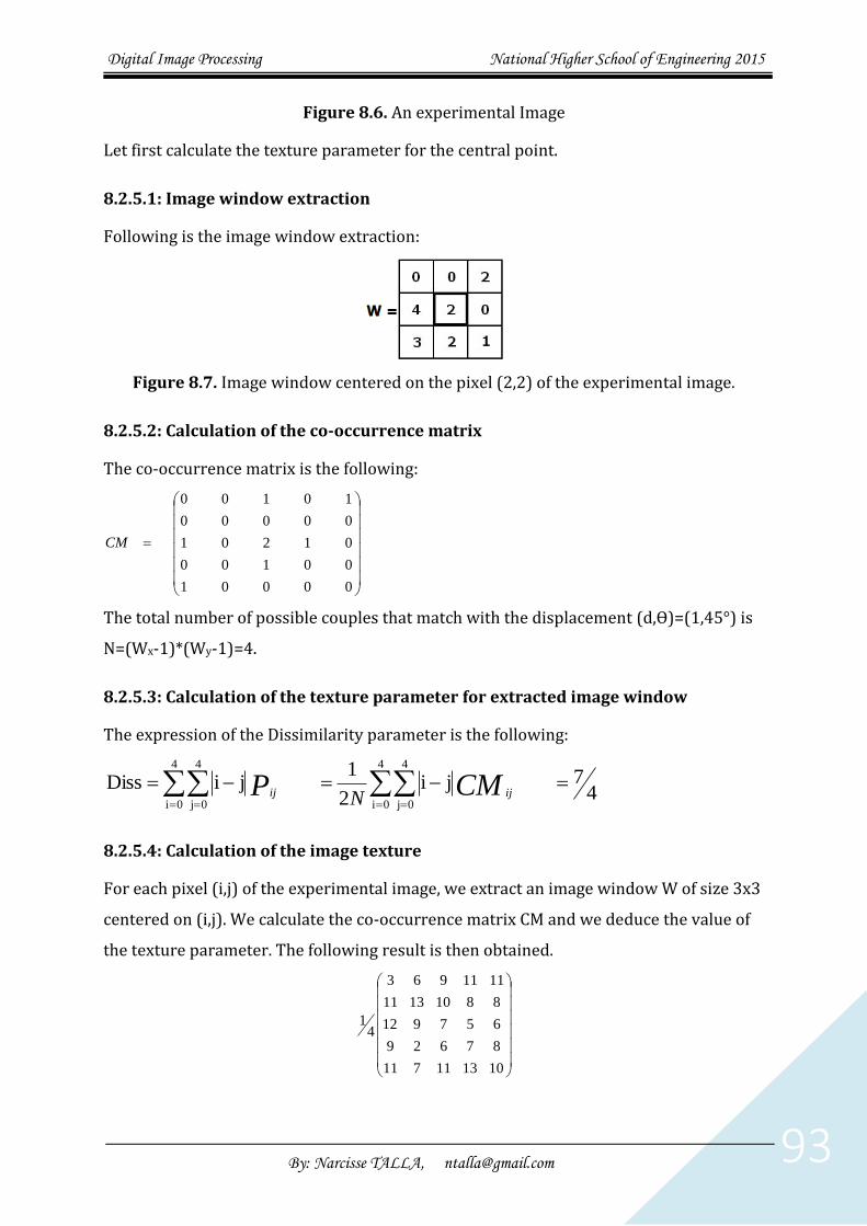
Digital Image Processing National Higher School of Engineering 2015
By: Narcisse TALLA, [email protected] 93
Figure 8.6. An experimental Image
Let first calculate the texture parameter for the central point.
8.2.5.1: Image window extraction
Following is the image window extraction:
Figure 8.7. Image window centered on the pixel (2,2) of the experimental image.
8.2.5.2: Calculation of the co-occurrence matrix
The co-occurrence matrix is the following:
00001
00100
01201
00000
10100
CM
The total number of possible couples that match with the displacement (d,Ɵ)=(1,45°) is
N=(Wx-1)*(Wy-1)=4.
8.2.5.3: Calculation of the texture parameter for extracted image window
The expression of the Dissimilarity parameter is the following:
47ji
2
1jiDiss
4
0i
4
0j
4
0i
4
0j
CMP ijij N
8.2.5.4: Calculation of the image texture
For each pixel (i,j) of the experimental image, we extract an image window W of size 3x3
centered on (i,j). We calculate the co-occurrence matrix CM and we deduce the value of
the texture parameter. The following result is then obtained.
101311711
87629
657912
88101311
1111963
41
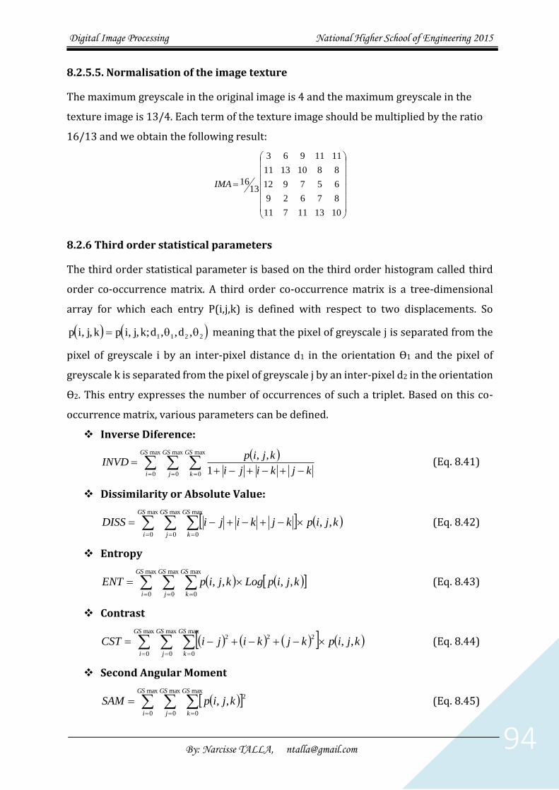
Digital Image Processing National Higher School of Engineering 2015
By: Narcisse TALLA, [email protected] 94
8.2.5.5. Normalisation of the image texture
The maximum greyscale in the original image is 4 and the maximum greyscale in the
texture image is 13/4. Each term of the texture image should be multiplied by the ratio
16/13 and we obtain the following result:
101311711
87629
657912
88101311
1111963
1316IMA
8.2.6 Third order statistical parameters
The third order statistical parameter is based on the third order histogram called third
order co-occurrence matrix. A third order co-occurrence matrix is a tree-dimensional
array for which each entry P(i,j,k) is defined with respect to two displacements. So
p i j k p i j k d d, , , , ; , , , 1 1 2 2 meaning that the pixel of greyscale j is separated from the
pixel of greyscale i by an inter-pixel distance d1 in the orientation Ɵ1 and the pixel of
greyscale k is separated from the pixel of greyscale j by an inter-pixel d2 in the orientation
Ɵ2. This entry expresses the number of occurrences of such a triplet. Based on this co-
occurrence matrix, various parameters can be defined.
Inverse Diference:
max
0
max
0
max
0 1
,,GS
i
GS
j
GS
k kjkiji
kjipINVD (Eq. 8.41)
Dissimilarity or Absolute Value:
max
0
max
0
max
0
,,GS
i
GS
j
GS
k
kjipkjkijiDISS (Eq. 8.42)
Entropy
kjipLogkjipENTGS
i
GS
j
GS
k
,,,,max
0
max
0
max
0
(Eq. 8.43)
Contrast
max
0
max
0
max
0
222,,
GS
i
GS
j
GS
k
kjipkjkijiCST (Eq. 8.44)
Second Angular Moment
max
0
max
0
max
0
2,,
GS
i
GS
j
GS
k
kjipSAM (Eq. 8.45)

Digital Image Processing National Higher School of Engineering 2015
By: Narcisse TALLA, [email protected] 95
Inverse Differential Moment
max
0
max
0
max
0222
1
,,GS
i
GS
j
GS
k kjkiji
kjipIDM (Eq. 8.46)
Correlation
kjip
kjiCOR
GS
i
GS
j
GS
k
kji,,
max
0
max
0
max
02
(Eq. 8.47)
Covariance
kjipkjiCOVGS
i
GS
j
GS
k
kji ,,max
0
max
0
max
0
(Eq. 8.48)
Variance
kjipiVARGS
i
GS
j
GS
k
i ,,max
0
max
0
max
0
(Eq. 8.49)
Maximal Probability
kjipMaxPGSkji
,,maxmax,,0
(Eq. 8.50)
Third Angular Moment
max
0
max
0
max
0
3,,
GS
i
GS
j
GS
k
kjipTAM (Eq. 8.51)
Importance of small numbers
max
0
max
0
max
0222
,,GS
i
GS
j
GS
k kji
kjipISN (Eq. 8.52)
Importance of great numbers
max
0
max
0
max
0
222 ,,GS
i
GS
j
GS
k
kjipkjiIGN (Eq. 8.53)
Importance of deepness
max
1
max
1
max
1
max
1
max
1
2max
1
,,
,,
GS
i
GS
j
GS
k
GS
i
GS
j
GS
k
kjip
kjip
ID (Eq. 8.54)
The value of 2 is given by:
kjipkji kj
GS
i
GS
j
GS
k
i ,,max
0
max
0
max
0
2
(Eq. 8.55)
Researchers don’t often use this method in remote sensing because of time and memory
space consuming.

Digital Image Processing National Higher School of Engineering 2015
By: Narcisse TALLA, [email protected] 96
8.3 Vegetation indices
Derived from remote sensing data, vegetation indices constitute a basic and precious
information for environment management. Accurate and opportune data collection on
world crops are constant preoccupation of human being. Collecting such data by in situ
techniques is onerous and time consuming when it is not simply impossible.
One approach consists in measuring the vegetation quantity and condition by
multispectral data analysis. Many studies in this area, using multispectral data, have been
developed, notably: Landsat MSS (Multispectral Scanner), Landsat TM (Thematic
Mapper), SPOT-HRV (High Visible Resolution) or NOAA-AVHRR (Advanced Very High
Resolution Radiometer). The aim often consists in transforming various bands into a
single image in which the value of a pixel predicts and measures environment
characteristics, such as the biomass, the productivity (photo mass) the Leaf Area Index
(LAI), the quantity of photosynthetic active radio (PAR) consumed or the percentage of
vegetation cover.