Chapter 0 Introduction:

0.1 Introduction to linear algebra:

Mathematics is the background of every engineering fields. Together with physics,

mathematics has helped engineering develop. Without it, engineering cannot have

evolved so fast we can see today.

Also mathematics is useful in so many areas because it is abstract: the same good

idea can unlock the problems of control engineers, civil engineers, physicists, social

scientists, and mathematicians only because the idea has been abstracted from a

particular setting. One technique solves many problems only because someone has

established a theory of how to deal with these kinds of problems.

We use definitions to try to capture important ideas, and we use theorems to

summarize useful general facts about the kind of problems we are studying. Proofs

not only show us that a statement is true; they can help us understand the

statement, give us practice using important ideas, and make it easier to learn a

given subject.

Without mathematics, engineering cannot become so fascinating as it is now.

numerical analysis (Which will be our subject), calculus, statistics, differential

equations and Linear algebra are taught as they are important to understand many

engineering subjects such as fluid mechanics, heat transfer, electric circuits,

Computer engineering and mechanics of materials to name a few.

it is accurate to say that a discrete math course and calculus indeed provides

sufficient mathematical background for a computer scientist and engineering

working in the “core” areas of the field, such as databases, compilers, operating

systems, architecture, and networks. Other mathematical issues no doubt arise

even in these areas, but peripherally and unsystematically; the computer scientist

can learn the math needed as it arises.

However, Numerical analysis can be defined as the development and

implementation of techniques to find numerical solution to mathematic,

Engineering and science problems. It also involves mathematics in developing

techniques for the approximate solution for the implementation of these

techniques in an optimal fashion for the particular computer programs. With the

accessibility of computers, it is now possible to get rapid and accurate solution to

many complex problems that create difficulties for, the mathematician, engineer

and scientist.

When engineering system are modeled, the mathematical description is developed

in term of sets of algebraic equation. Sometime these equations are linear and

sometime nonlinear. In first part we discuss systems of linear equation and how to

solve them using direct methods.

However, The solution of a system of linear algebraic equation probably one of the

most important topic in engineering computations.

In second part we will study one of the most fundamental problems of numerical

analysis, namely the numerical solution of nonlinear equations. Where most

equations are arising in practice are nonlinear and are of a form that allows the

roots to be determined exactly. Consequently, numerical methods are used to

solve nonlinear equations when the equations prove intractable to ordinary

mathematical techniques. These numerical methods are all iterative. At part three

we will describe numerical methods for the approximation of functions other than

elementary functions. Where the main purpose of these techniques is to replace a

complicated function by one that simpler and more manageable. Finally, in part

four we will deal with techniques for approximating numerically the two

fundamental operations of calculus, differentiation and integrations. Both of these

problems may be approached in the same way. Although both numerical

differentiation and numerical integration formulas will be discussed.

What does the term linear equation mean?

An equation is where two mathematical expressions are defined as being equal. A

linear equation is one where all the variables such as

x, y, z

have index (power) of 1 or 0 only,

for example

x + 2y + z = 5

is a linear equation. The following are also linear equations:

x = 3;

x + 2y = 5;

3x + y + z + w = −8

The following are not linear equations:

1. 𝑥2 − 1 = 0

2. 𝑥 + 𝑦4 + √𝑧 = 9

3. sin(x) − y + z = 3

Why not?

In equation (1) the index (power) of the variable x is 2, so this is actually a quadratic

equation.

In equation (2) the index of y is 4 and z is 1/2.

In equation (3) the variable x is an argument of the trigonometric function sine.

Note that if an equation contains an argument of trigonometric, exponential,

logarithmic or hyperbolic functions then the equation is not linear.

A set of linear equations is called a linear system.

In this course on linear algebra we examine the following questions regarding

linear systems:

● Are there any solutions?

● Does the system have no solution, a unique solution or an infinite number of

solutions?

● How can we find all the solutions, if they exist?

● Is there some sort of structure to the solutions?

Linear algebra is a systematic exploration of linear equations and is related to ‘a

new kind of arithmetic’ called the arithmetic of matrices which we will discuss later

in the chapter.

However, linear algebra isn’t exclusively about solving linear systems. The tools of

matrices and vectors have a whole wealth of applications in the fields of functional

analysis and quantum mechanics, where inner product spaces are important. Other

applications include optimization and approximation where the critical questions

are:

1. Given a set of points, what’s the best linear model for them?

2. Given a function, what’s the best polynomial approximation to it?

To solve these problems, we need to use the concepts of eigenvalues and

eigenvectors and orthonormal bases which are discussed in later chapters. In all of

mathematics, the concept of linearization is critical because linear problems are

very well understood and we can say a lot about them. For this reason, we try to

convert many areas of mathematics to linear problems so that we can solve them.

Linear algebra is essentially the study of vectors, matrices, and linear mappings.

Many of the concepts introduced in linear algebra are natural and easy, but some

may seem unnatural and "technical" to beginners. Do not avoid these apparently

more difficult ideas; use examples and theorems to see how these ideas are an

essential part of the story of linear algebra.

0.2 Introduction to matrix:

Engineering Mathematics is applied in our daily life. Applied Mathematics is future

classified as vector algebra, differential calculus, integration, discrete Mathematics,

Matrices etc. Matrices are one of the most powerful tools in mathematics. The

evolution of the concept of matrices is the result of an attempt to obtain compact

and simple methods of solving the system of linear equations.

Matrices have a long history of application in solving linear equations. The first

example of the use of matrix methods to solve simultaneous equations, including

the concept of determinants. In this semester we will study overview of application

of matrices in engineering and science.

A Matrices is a two dimensional arrangement of numbers in row and column

enclosed by a pair of square brackets or can say matrices are nothing but the

rectangular arrangement of numbers, expression, symbols which are arranged in

column and rows. Matrices find many applications in scientific field and apply to

practical real life problem.

The scientist understand that the originality of matrix came from the study of

system of simultaneous linear equation.

0.3 Applications of Matrices:

Matrices have many applications in diverse fields of science, commerce and social

science. Matrices are used.

1- Use of Matrices in Computer Graphics

Matrix transforms are very useful within the world of computer graphics,

Software and hardware graphics processor uses matrices for performing

operations such as scaling translation, reflection and rotation.

In video gaming industry matrices are major mathematical tool to construct and

manipulate a realistic animation of a polygonal figure. Computer graphics software

uses matrices to process linear transformations to translate images. For this

purpose, square matrices are very easily representing linear transformation of

objects.

Matrices can play a vital role in the projection of three dimensional images into

two dimensional screens, creating the realistic decreeing motion. In Graphics,

digital image is treated as a matrix to be start with. The rows and columns of matrix

correspond to rows and columns of pixels and the numerical entries correspond

to the pixels’ color values.

Now day’s matrices are used in the ranking of web pages in the Google search. It

can also be used in generalization of analytical motion like experimental &

derivatives to their high dimensional.

2- Use of matrices in cryptography:

The most important usages of matrices in computer side application are

encryption of message codes with the help of encryptions only, internal function

are working and even could work with transmission of sensitive & private data.

Cryptography is the technique to encrypting data so that only the relevant person

can get the data and relate information. In earlier days, video signals were not

used to encrypt. Anyone with satellite dish was able to watch videos which results

in the loss for satellite owners, so they started encrypting the video signals so that

only those who have videos cipher can unencryptedthe signals.

This encrypting is done by using an invertible key is not invertible then the

encrypted signals cannot be unencrypted and they cannot get back to original

form. This process is done using matrices.

A digital audio or video signal is firstly taken as a sequence of numbers

representing the variation over time of air pressure of an acoustic audio signal.

The filtering techniques are used which depends on matrix multiplication.

3- Use of Matrices in Wireless Communication

Matrix Cramer’s Rule and determinants are simple and important tools for solving

many problems in business and economics related to maximize profit and

minimize loss. Matrices are used to find variance and co- variance.

4- Use in data analysis:

Matrices are very useful for organization, like for scientists who have to record

data form their experiments if it includes numbers.

In engineering reports are recorded using matrices

5- Matrices for Financial Records:

Matrices allow to represent array of many numbers as a single object and is

denoted by a single symbol then calculations are performed on these symbols

in very compact form. The matrix method of obtaining opening and closing

balances for any accounting period is very efficient, accurate and less time

consuming.

6- Matrices for Engineering:

Matrices applications involve the use of Eigen values and Eigen vectors in the

process of transforming a given matrix into a diagonal matrix. Linear algebra is

useful tool for solving large number of variables in such a short time. It is

interesting to note that many of the calculus theorems used in engineering classes

are proved quickly and easily through linear algebra.

Transformation matrices are commonly used in computer graphics and image

processing.

7- Matrices are used in robotics & automation:

in terms of base elements for the robot movements. The movements of the robots

are programmed with the calculation of matrices ‘row &column “Controlling of

matrices are done by calculation of matrices.

8- Also matrices are also used in geology for seismic survey and it is also used for

plotting graphs.

Matrices used in Statistics plays a vital role in scientific studies.

Chapter 1: Introduction to system of linear equation:

Connecting theory and application is a challenging but important problem. This is

important for all students. We need to motivate our engineering students so they

can be successful in their educational and occupational lives. Linear systems of

equations naturally occur in many places in engineering, such as structural analysis,

dynamics and electric circuits. Computers have made it possible to quickly and

accurately solve larger and larger systems of equations. Not only has this allowed

engineers to handle more and more complex problems where linear systems

naturally occur, but has also prompted engineers to use linear systems to solve

problems where they do not naturally occur such as thermodynamics, strain

analysis, fluids and chemical processes. It has become standard practice in many

areas to analyze a problem by transforming it into a linear systems of equations

and then solving those equations by computer.

In this way, computers have made linear systems of equations the most frequently

used tool in modern engineering.

1.1 System of linear equations

Recall that the general equation of a line in 𝑅2 is of the form

𝑎𝑥 + 𝑏𝑦 = 𝑐

and that the general equation of a plane in 𝑅3 is of the form

𝑎𝑥 + 𝑏𝑦 + 𝑐𝑧 = 𝑑

Equations of this form are called linear equations.

Definition : A linear equation in the n variables 𝑥1, 𝑥2 , … . , 𝑥𝑛 is an equation that

can be written in the form

𝑎1𝑥1 + 𝑎2𝑥2 + ⋯ + 𝑎𝑛𝑥𝑛 = 𝑏

where the coefficients 𝑎1, 𝑎2 , … , 𝑎𝑛 and the constant term b are constants.

For example, the following system has four equations and three variables:

3𝑥1 − 2𝑥2 − 5𝑥3 = 4

2𝑥1 + 4𝑥2 − 𝑥3 =2

6𝑥1 − 4𝑥2 − 10𝑥3 = 8

−4𝑥1 + 8𝑥2 + 9𝑥3 = −6

We often need to find the solutions to a given system. The ordered triple, or 3-

tuple, (𝑥1, 𝑥2, 𝑥3) = (4, −1, 2) is a solution to the preceding system because each

equation in the system is satisfied for these values of 𝑥1, 𝑥2, and 𝑥3. Notice that

(−3

2 ,

3

4 , −2) is another solution for that same system. These two particular

solutions are part of the complete set of all solutions for that system. We now

formally define linear systems and their solutions.

The system of m linear equation in n variables𝑥1, 𝑥2, 𝑥3,… …, 𝑥𝑛 is of the form

𝑎11𝑥1+𝑎12𝑥2 + ⋯ ⋯ + 𝑎1𝑛𝑥𝑛 = 𝑏1

𝑎11𝑥1+𝑎12𝑥2 + ⋯ ⋯ + 𝑎1𝑛𝑥𝑛 = 𝑏1

⋮ ⋮ + ⋯ ⋯ + ⋮ = ⋮

𝑎𝑚1𝑥1+𝑎𝑚2𝑥2 + ⋯ ⋯ + 𝑎𝑚𝑛𝑥𝑛 = 𝑏𝑚

1.2 Solving linear systems using Gaussian eliminations:

In this section, we introduce a method for solving such systems known as Gaussian

Elimination.

Example:

𝑥 + 2𝑦 + 𝑧 = 1

3𝑥 + 𝑦 + 4𝑧 = 0

2𝑥 + 2𝑦 + 3𝑧 = 2

is a linear system in the variables x, y, and z.

Finding all solutions to this system is not hard. We begin by subtracting three times

the first equation from the second, producing.

𝑥 + 2𝑦 + 𝑧 = 1

− 5𝑦 + 𝑧 = 0

2𝑥 + 2𝑦 + 3 𝑧 = 2

Any x, y, and z that satisfy the original system also satisfy the system above. Thus

both systems have the same solution set. We say that these systems are equivalent.

Definition: Two systems of linear equations in the same variables are equivalent if

they have the same solution set.

To continue the solution process, we next subtract twice the first equation from

the third, producing.

𝑥 + 2𝑦 + 𝑧 = 1

− 5𝑦 + 𝑧 = −3

− 2𝑦 + 𝑧 = 0

Note that we have eliminated all occurrences of x from the second and third

equations. This system is equivalent with our second system for similar reasons

that the second system was equivalent with the first. It follows that this system has

the same solution set as the original system.

Next, we eliminate y from the third equation by subtracting twice the second from

five times the third, again producing an equivalent system:

𝑥 + 2𝑦 + 𝑧 = 1

− 5𝑦 + 𝑧 = −3

3 𝑧 = 6

Thus, z = 2. Then, from the second equation, y = 1, and finally, from the first

equation, x = −3. Thus, our only solution is [−3, 1, 2].

The fact that there was only one solution can be understood geometrically.

Remark. The method we used to compute the solution from system (1.11) is

referred to as back substitution. In general, in back substitution, we solve the last

equation for one variable and then substitute the result into the preceding

equations, obtaining a system with one fewer variable and one fewer equation, to

which the same process may be repeated. In this way, we obtain all solutions to the

system.

The process we used to reduce system (1) to system (2) is called Gaussian

elimination. The general idea is to use the first equation to eliminate all occurrences

of the first variable from the equations below it.

One then attempts to use the second equation to eliminate the next variable from

all equations below it, and so on. In the end, the last variable is determined first

and then the others are determined by substitution as in the example.

We will describe Gaussian elimination in detail in the next chapter, after we

introduce the notion of Matrix.

The system solved in Example 3 is a particularly simple one. However, the solution

procedure introduces all the steps that are needed in the process of elimination.

They are worth reviewing. Types of Steps in Elimination

(1) Multiply one equation by a non-zero constant.

(2) Interchange two equations.

(3) Add a multiple of one equation to another equation.

Our approach to solving a system of linear equations is to transform the given

system into an equivalent one that is easier to solve. The triangular pattern of the

second example above (in which the second equation has one less variable than

the first) is what we will aim for.

Ex: Finding the solutions to this given system

𝑥 + 2𝑦 + 4𝑧 = 7

3𝑥 + 7𝑦 + 2𝑧 = −11

2𝑥 + 3𝑦 + 3𝑧 = 1

1.3 Types of solutions

We now go back to evaluating a simple system of two linear simultaneous

equations and discuss the case where we have no, or an infinite number of

solutions. As one of the fundamental questions of linear algebra is how many

solutions do we have of a given linear system.

The graphs represent the three possible solutions to a linear system with two

unknowns.

Example: Solve the following systems of linear equations:

1- 𝑥 + 𝑦 = 6 2- 𝑥 + 𝑦 = 2 3- 𝑥 + 𝑦 = 6

−𝑥 + 𝑦 = 2 𝑥 + 𝑦 = 6 2𝑥 + 2𝑦 = 12

Solution :

1- Adding the two equations together gives 2y = 8, so y = 4, from which we find

that x= 2. A quick check confirms that [2, 4] is indeed a solution of both

equations. That this is the only solution can be seen by observing that this

solution corresponds to the (unique) point of intersection.

2- Two numbers x and y cannot simultaneously have a sum of 2 and 6. Hence,

this system has no solutions. As Figure (2) shows, the lines for the equations

are parallel in this case

3- The second equation in this system is just twice the first, so the solutions are

the solutions of the first equation alone-namely, the points on the line x + y

= 6. These can be represented parametrically as [2 + t, t] . Thus, this system

has infinitely many solutions [Figure (3)].

Note: A system of linear equations is called consistent if it has at least one

solution. A system with no solutions is called inconsistent. Even though they are

small, the three systems in above Example illustrate the only three possibilities

for the number of solutions of a system of linear equations with real coefficients.

Ex: Solve the following systems of linear equations and explain the types using

presentation graph :

1- 2𝑥 + 2𝑦 = 4 2- 2𝑥 − 𝑦 = −3 3- 3𝑥 + 𝑦 = 1

2𝑥 − 𝑦 = 8 4𝑥 − 2𝑦 = −6 3𝑥 + 𝑦 = 5

Note: Systems of equations are a very useful tool for modeling real-life situations

and answering questions about them. If you can translate the application into two

linear equations with two variables or more, then you have a system of equations

that you can solve to find the solution. You can use any method to solve the system

of equations.

Example : Suppose you want to know the win/loss record of your favorer football

team. You know they played 24 games during the season, and you also know that

they won 15 more games than they lost. We are looking for the number of wins

and the number of losses, so we have two unknowns.

Note: Systems of equations are used to solve applications when there is more than

one unknown and there is enough information to set up equations in those

unknowns. In general, if there are n unknowns, we need enough information to set

up n equations in those unknowns.

Solution: The first thing we want to do is represent our unknowns using variables. Let's let

x = number of wins and

y= number of losses.

We are given that the team played 24 games total. We know that the number of wins plus the number of losses has to equal the total number of games played. Therefore,

x + y = 24.

We have our first equation.

Since there are two unknowns, we know we want one more equation. We are told that the team won 15 more games than they lost. This tells us that the number of losses plus 15 would give the number of wins.

Putting that in equation form, we have that

y + 15 = x.

We have our second equation, so we have our system of equations.

x + y = 24.

-x + y = -15.

Note: One application of system of equations are known as value problems. Value problems are ones where each variable has a value attached to it.

Ex: the marketing team for an event venue wants to know how to focus their advertising based on who is attending specific events—children, or adults? They know the cost of a ticket to a basketball game is $20.00 for children and $30.00 for adults.

Additionally, on a certain day, attendance at the game is 4,000 and the total gate revenue is $80,000. How can the marketing team use this information to find out whether to spend more money on advertising directed toward children or adults?

Ex: A total of $8,300 was invested in two accounts. Part was invested in a computer at a 4% annual interest rate and part was invested in a money market fund at a 5% annual interest rate. If the total simple interest for one year was $260, then how much was invested in each account.

Ex: A farmer has three types of milk, one that is 24% butterfat, 15% butterfat and another which is 18% butterfat. How much of each should he use to end up with 44 gallons of 25% butterfat.

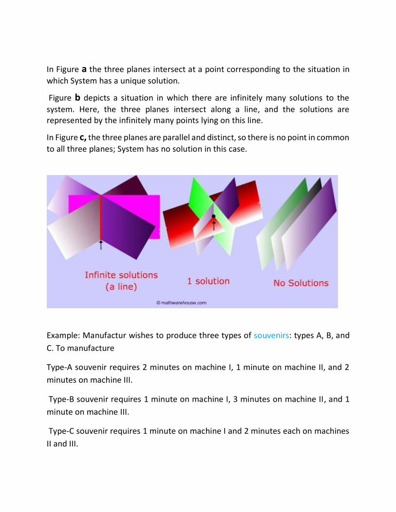
In Figure a the three planes intersect at a point corresponding to the situation in

which System has a unique solution.

Figure b depicts a situation in which there are infinitely many solutions to the

system. Here, the three planes intersect along a line, and the solutions are represented by the infinitely many points lying on this line.

In Figure c, the three planes are parallel and distinct, so there is no point in common

to all three planes; System has no solution in this case.

Example: Manufactur wishes to produce three types of souvenirs: types A, B, and

C. To manufacture

Type-A souvenir requires 2 minutes on machine I, 1 minute on machine II, and 2

minutes on machine III.

Type-B souvenir requires 1 minute on machine I, 3 minutes on machine II, and 1

minute on machine III.

Type-C souvenir requires 1 minute on machine I and 2 minutes each on machines

II and III.

There are 3 hours available on machine I, 5 hours available on machine II, and 4

hours available on machine III for processing the order. How many souvenirs of

each type should make in order to use all of the available time? Formulate and

solve the problem.

Solution: The given information may be tabulated as follows.

Type A Type B Type C Time Available (min)

Machine I 2 1 1 180

Machine II 1 3 2 300

Machine III 2 1 2 240

We have to determine the number of each of three types of souvenirs to be made.

So, let x, y, and z denote the respective numbers of type-A, type-B, and type-C

souvenirs to be made.

The total amount of time that machine I is used is given by 2x + y+ z minutes and

must equal 180 minutes. This leads to the equation

2𝑥 + 𝑦 + 𝑧 = 180 Time spent on machine I

Similar considerations on the use of machines II and III lead to the following

equations:

𝑥 + 3𝑦 + 2𝑧 = 300 Time spent on machine II

2𝑥 + 𝑦 + 2𝑧 = 240 Time spent on machine III

Then the solution to the problem is found by solving the following system of linear

equations: illustrates each of these possibilities.

2𝑥 + 𝑦 + 𝑧 = 180

𝑥 + 3𝑦 + 2 𝑧 = 300

2𝑥 + 𝑦 + 2𝑧 = 240

Chapter 2: Introduction to Matrices and Matrix algebra

2.1 Introduction:

Information in science, business, engineering and mathematics is often organized

into rows and columns to form rectangular arrays called “matrices” (plural of

“matrix”). Matrices often appear as tables of numerical data that arise from

physical observations, but they occur in various mathematical contexts as well. For

example, we will see in the coming chapters that all of the information required to

solve a system of linear equations such as

5𝑥 + 𝑦 = 3

2𝑥 − 𝑦 = 4

is embodied in the matrix

(5 1 ⋮ 32 −1 ⋮ 4

)

and that the solution of the system can be obtained by performing appropriate

operations on this matrix. This is particularly important in developing computer

programs for solving systems of equations because computers are well suited for

manipulating arrays of numerical information.

However, matrices are not simply a notational tool for solving systems of

equations; they can be viewed as mathematical objects in their own right, and

there is a rich and important theory associated with them that has a multitude of

practical applications. It is the study of matrices and related topics that forms the

mathematical field that we call “linear algebra and Analysis.” In this chapter we will

begin our study of matrices.

Image and its Matrix:

There is a relation between matrices and digital images. A digital image in a

computer is presented by pixels matrix. On the other hand, there is a need

(especially with high dimensions matrices) to present matrix with an image.

The images you see on internet pages and the photos you take with your mobile

phone are examples of digital images. It is possible to represent this kind of image

using matrices. For example, the small image of Felix the Cat

can be represented by a

35×35 matrix

whose elements are the numbers 0 and 1. These numbers specify the color of each

pixel1: the number 0 indicates black, and the number 1 indicates white. Digital

images using only two colors are called binary images.

Grayscale images can also be represented by matrices. Each element of the matrix

determines the intensity of the corresponding pixel.

Note: A pixel is the smallest graphical element of a matricial image, which can take

only one color at a time

For convenience, most of the current digital files use integer numbers between 0

(to indicate black, the color of minimal intensity) and 255 (to indicate white,

maximum intensity), giving a total of

256 = 28

different levels of gray.

For example, the image is presented with the matrix

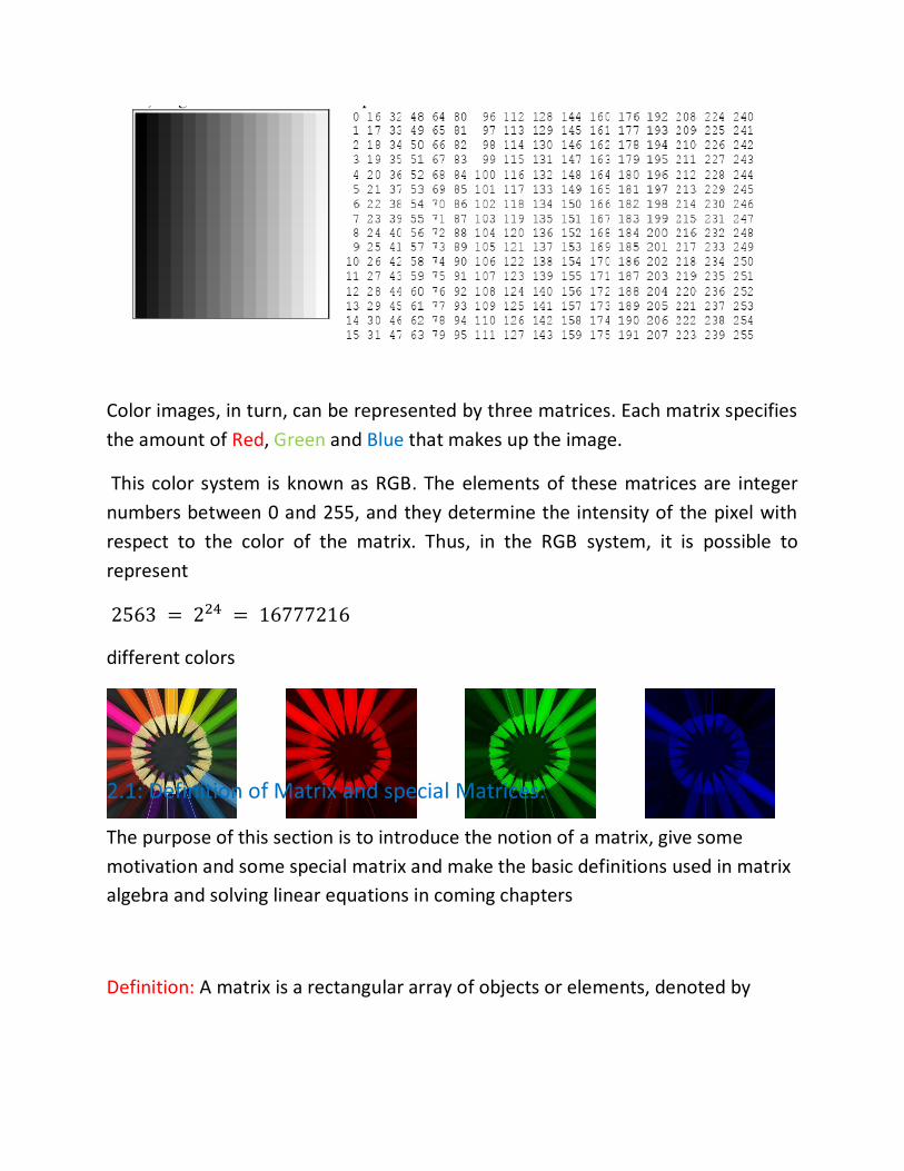
Color images, in turn, can be represented by three matrices. Each matrix specifies

the amount of Red, Green and Blue that makes up the image.

This color system is known as RGB. The elements of these matrices are integer

numbers between 0 and 255, and they determine the intensity of the pixel with

respect to the color of the matrix. Thus, in the RGB system, it is possible to

represent

2563 = 224 = 16777216

different colors

2.1: Definition of Matrix and special Matrices:

The purpose of this section is to introduce the notion of a matrix, give some

motivation and some special matrix and make the basic definitions used in matrix

algebra and solving linear equations in coming chapters

Definition: A matrix is a rectangular array of objects or elements, denoted by

A ∶= [

𝑎11 𝑎12 … 𝑎1𝑛

𝑎21 𝑎22 … 𝑎2𝑛

⋮ ⋮ ⋱ ⋮𝑎𝑚1 𝑎𝑚2 𝑎𝑚𝑛

]

The displayed matrix has (m) rows and (n) columns and is called an m by n matrix

or matrix of order (m × n).

1. The size of the matrix is denoted by (m × n).

2. Each entry in the matrix is called the entry or elements of the matrix and is

denoted by (aij ), where (i) is the row number and (j) is the column number

of the element.

Example :

A = [2 1 3 41 3 0 24 3 5 6

]

There are (3) rows and (4) columns, so the size of A is (3×4) and (a23 = 0) ,

(a32 = 3).

1- Square matrix: is a matrix where number of row = number of column.

2- Symmetric matrix: is a square matrix where (aij = aji) for all(i ≠ j).

Example :

B = [o 32 5

] is (2×2) square matrix but not symmetric.

Example :

C = [1 4 64 1 06 0 3

] is (3×3) square and symmetric matrix by

(a12 = a21 = 4),(a13 = a31 = 6) and (a23 = a32 = 0).

3- Diagonal( main) of the matrix: are given by the elements (aij) for i = j

that is all a11 , a22 , a33 ⋯.

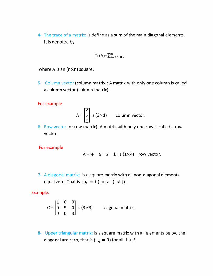
4- The trace of a matrix: is define as a sum of the main diagonal elements.

It is denoted by

Tr(A)=∑ aiini=1 ,

where A is an (n×n) square.

5- Column vector (column matrix): A matrix with only one column is called

a column vector (column matrix).

For example

A = [270

] is (3×1) column vector.

6- Row vector (or row matrix): A matrix with only one row is called a row

vector.

For example

A =[4 6 2 1] is (1×4) row vector.

7- A diagonal matrix: is a square matrix with all non-diagonal elements

equal zero. That is (aij = 0) for all (i ≠ j).

Example:

C = [1 0 00 5 00 0 3

] is (3×3) diagonal matrix.

8- Upper triangular matrix: is a square matrix with all elements below the

diagonal are zero, that is (aij = 0) for all i > 𝑗.

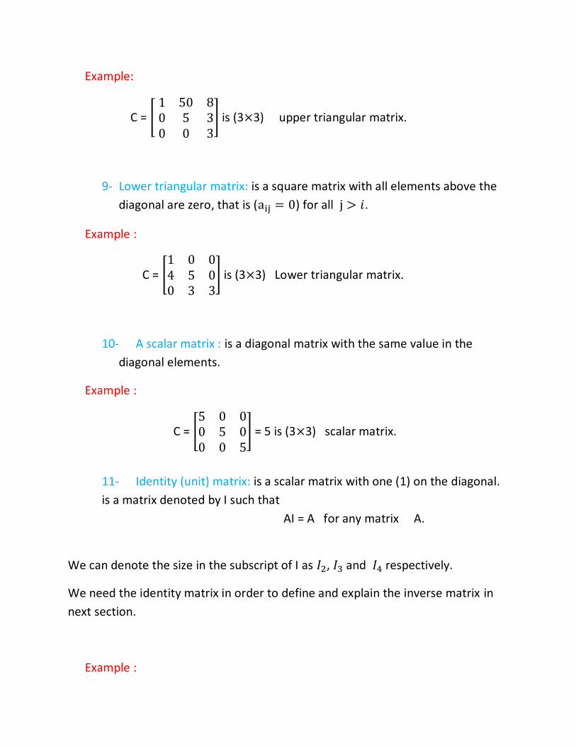
Example:

C = [ 1 50 80 5 30 0 3

] is (3×3) upper triangular matrix.

9- Lower triangular matrix: is a square matrix with all elements above the

diagonal are zero, that is (aij = 0) for all j > 𝑖.

Example :

C = [1 0 04 5 00 3 3

] is (3×3) Lower triangular matrix.

10- A scalar matrix : is a diagonal matrix with the same value in the

diagonal elements.

Example :

C = [5 0 00 5 00 0 5

] = 5 is (3×3) scalar matrix.

11- Identity (unit) matrix: is a scalar matrix with one (1) on the diagonal.

is a matrix denoted by I such that

AI = A for any matrix A.

We can denote the size in the subscript of I as 𝐼2, 𝐼3 and 𝐼4 respectively.

We need the identity matrix in order to define and explain the inverse matrix in

next section.

Example :

C = [1 0 00 1 00 0 1

] = I is (3×3) Identity matrix.

12- Zero (null) matrix: Is the matrix all of whose elements are zero. There

is a zero matrix for every size.

For example

C = [0 0 00 0 00 0 0

] = 0 is (3×3) zero matrix and [0 0 00 0 0

] is (2×3) zero

matrix.

2.2 matrix operation

1. Equality of two matrices: Two matrices A and B are equal if the size of A

and B is the same . That is ( 𝑎𝑖𝑗 = 𝑏𝑖𝑗) for all i and j.

For example

If [𝑥 43 𝑦

] = [2 43 1

] then 𝑥 = 2 and 𝑦 = 1 .

2. Addition of matrices: The operation of addition of two matrices is only

defined when both matrices have the same size (dimensions). If A and B are

both (m × n), then the sum

C =A+B

is also (m × n) and is defined to have each element the sum of the

corresponding elements of A and B, thus

𝑐𝑖𝑗 = 𝑎𝑖𝑗 + 𝑏𝑖𝑗 .

The subtraction of two matrices is similarly defined; if A and B have the

same dimensions, then the difference

C =A-B

By the same way of addition, implies that the elements of C are

𝑐𝑖𝑗 = 𝑎𝑖𝑗 − 𝑏𝑖𝑗.

For example:

[−2 42 0

] + [2 43 1

] = [−2 + 2 4 + 42 + 3 0 + 1

] = [0 85 1

]

[2 43 1

] + [3 7 24 5 1

] is not define

Basic Properties of Matrices addition

Matrix addition is commutative: A + B = B + A

Matrix addition is associative: A + (B + C) = (A + B) + C

3. Multiplication of a matrix by a number (scalar multiplication): There is also

a natural way of defining the product of a matrix with a number. Using the

matrix A= [2 43 1

] , we note that

A+A=[2 43 1

] + [2 43 1

] = [4 86 2

] =2 A.

What we see is that 2A (which is the shorthand notation for A+A) is obtained

by multiplying every element of A by 2, where a scalar is a number which is

used to multiply the entries of a matrix

In general if A is an (m × n) matrix with typical element (𝑎𝑖𝑗) then the product

of a number k with A written (kA) is the product B = kA is defined to be the

matrix of the same dimensions as A whose elements are simply all scaled by

the constant k

𝑏𝑖𝑗 = 𝑘 × 𝑎𝑖𝑗 .

For example:

3 [−2 42 0

] = [3 × −2 3 × 43 × 2 3 × 0

] = [−6 126 0

].

The distributive law holds: k(A + B) = k A + k B where k real number.

4. Matrix Multiplication: Two matrices may be multiplied together only if

they meet conditions on their dimensions that allow them to conform as

following.

Let A have dimensions (m × n) and B be (n × p), that is A has the same number

as columns as the number of rows in B, then the product

C =AB,

is defined to be an (m × p) matrix with elements

𝑐𝑖𝑗 = ∑ 𝑎𝑖𝑘𝑏𝑘𝑗𝑛𝑘=1 .

The element in position (𝑖𝑗) is the sum of the products of elements in the i-th

row of the first matrix (A) and the corresponding elements in the j-th column

of the second matrix (B).

Notice that the product AB is not defined unless the above condition is

satisfied, that is the number of columns of the first matrix must equal the

number of rows in the second.

For example:

[−2 42 0

] [3 15 0

] = [(−2 × 3) + (4 × 5) (−2 × 1) + (4 × 0)

(2 × 3) + (0 × 5) (2 × 1) + (0 × 0)] = [

14 −26 2

].

[−2 42 0

] [4 47 20 1

] is not define.

Matrix multiplication is associative, that is A (BC)=(AB) C.

Matrix multiplication Distributive over addition A(B + C) = AB + AC

(B + C) A = BA + CA

But is not commutative in general AB ≠ BA.

Consider the

Example:

A=[1 21 2

] and B=[0 12 0

]

It is interesting to note that unlike the scalar case, the fact that AB = 0 does not

imply that either A = 0 or that B = 0.

Exercise :

Let A=[6 32 5

] and B=[2 43 1

], then find the followings

1- 3A+2B 2- -4A+B2.

2- Show that by example (𝐴 − 𝐵)2 = 0 does not imply A=B

Example : A computer monitor with (640) row pixels and (480) column can

viewed as a matrix. In order to create an image, each pixel is filled with an

appropriate colure.

The following example demonstrates the practical application of matrix

multiplication.

A local computer office shop sells three types of Laptop : Dell, Lenovo and HP. Dell

costs $260 each, Lenovo $300 each and HP $280 each. The sales of each Laptop

are as shown in Table

Sun Mon Tues Wed Thur

Dell 2 3 1 2 4

Lenovo 3 3 3 2 4

HP 2 3 4 2 4

Of course, you can solve this problem without matrices, but using matrix notation

provides a systematic way of evaluating the sales for each day.

Writing out the matrices and carrying out the matrix multiplication row by column

gives:

( 260 300 280) (2 3 1 2 43 3 3 2 42 3 4 2 4

) = (1980 2520 2280 1680 3360)

Hence the takings for Sunday are:

(2 × 260) + (3 × 300) + (2 × 280) = $1980.

Similarly for the other days, we have Monday $2520 Tuesday $2280, Wednesday

$1680 and Thursday $3360. The matrix on the right hand side gives the takings for

each weekday.

A software package such as MATLAB can be used for computing matrices. In fact,

MATLAB is short for ‘Matrix Laboratory’. It is a very useful tool which can be used

to eliminate the drudgery from lengthy calculations.

There are many mathematical software packages such as MAPLE and

MATHEMATICA, but MATLAB is particularly useful for linear algebra.

2.3 Unary Matrix operations

2.3.1 The Transpose of a Matrix

The transpose of an (m×n) matrix A, denoted 𝐴𝑇, is the (n×m) matrix define by

interchanging the rows and columns of A.

In general, the entry 𝑎𝑖𝑗 (ith row by jth column) of matrix A is transposed to 𝑎𝑗𝑖

(jth row by ith column) in 𝐴𝑇.

For example, if

A=[6 32 5

] then 𝐴𝑇=[6 23 5

]

Properties of Transposed Matrices

1- (𝐴 + 𝐵)𝑇 = 𝐴𝑇 + 𝐵𝑇.

2- (𝐴𝐵)𝑇 = 𝐵𝑇𝐴𝑇.

3- ((𝐴)𝑇)𝑇 = 𝐴.

Note: There are two important quantities associated with a square matrix. One is

the trace and the other is the determinant.

2.3.2 The Determinant of a Matrix:

The determinant of a matrix is a special number that can be calculated from or

defining only for square matrix, denoted by

det(A) or |𝐴|.

We will avoid the formal definition of the determinant (that implies notions

of permutations) for now and we will concentrate instead on its

calculation.

Finding the determinant depends on the dimension of the matrix, The

determinant of a matrix of size (n × n) is defined recursively in terms of

lower order determinants

((n − 1) × (n − 1)).

i. The determinant of (1×1) matrix or scalar matrix is the only number

in matrix. For example, det ([2])=2.

ii. The determinant of (2×2) matrix is defined by the relation

A=[a11 a12

a21 a22], then det (A)= a11a22 − a12a21.

For example

𝐴 = [−2 42 0

], then det (A)=-2×0-4×2=-8.

iii. The determinant of (3×3) matrix is defined by the relation.

A = [

a11 a12 a13

a21 a22 a23

a31 a32 a33

], then

det (A)= a11(a22 a33 − a23 a32) − a12(a21 a33 − a23 a31) + a11(a21 a32 −

a22a31).

For example

𝐴 = [3 2 10 1 25 4 2

],then det (A)=3(1×2--4×2)−2(0×2−2×5)+1(0×4−1×5)=18+20-5=33

We can simplify the way for finding determinant of (3×3) matrix as follows.

a) Rewrite the 1-st and 2-nd columns of A on the right (as “Columns 4 and 5”).

b) Add the products along the three main diagonals that extend from upper

left to lower right.

c) Subtract the products along the three secondary diagonals that extend

from lower left to upper right.

That is if A= [

a11 a12 a13

a21 a22 a23

a31 a32 a33

], to find det (A) we rewrite A as

[

a11 a12 a13 ⋮ a11 a12 a21 a22 a23 ⋮ a21 a22

a31 a32 a33 ⋮ a31 a32

]. Then

det (A)= (a11a22a33 )+ (a12a23a31 )+ (a13a21a32 )− (a13a22a31 )− (a11a23a32 )

− (a12a21a33 ).

Note: The determinant helps us find the inverse of a matrix, tells us things about

the matrix that are useful in systems of linear equations.

To finding the determinant in general of (n×n) matrix we need define the

following concepts first.

a/ Minor: The Minor of the element (𝑎𝑖𝑗), is denote by 𝑀𝑖𝑗 , is define to be the

determinant of the low dimension matrix (sunmatrix) formed by eliminate the i-th

row and j-th column in the original matrix.

For example

Let 𝐴 = [3 2 10 1 25 4 2

], then find 𝑀22 and 𝑀12

Solution: after eliminate the 2-nd row and 2-nd column in A we obtain

𝑀22=det([3 15 2

])=|3 15 2

|=(3×2)−(1×5)=1.

𝑀12=det([0 25 2

])=|0 25 2

|=(0×2)−(2×5)=−10.

b/ Cofactor: The cofactor of the element (𝑎𝑖𝑗), is denote by 𝐶𝑖𝑗, is defined by the

relation.

𝐶𝑖𝑗 = (−1)𝑖+𝑗𝑀𝑖𝑗.

Note: You will notice that the cofactor and the minor always have the same

numerical value, with the possible exception of their sign came from element

position.

For example :

In example above find 𝐶33 and 𝐶12

Solution: 𝐶33 = (−1)3+3𝑀33=|3 20 1

|=(3×1)−(2×0)=3.

𝐶12 = (−1)1+2𝑀33=−(−10)=10.

Now we are ready to give general formula for finding determinant of (n×n) matrix

using cofactor.

Let A be an (n×n) matrix, then determinant of A ( by choosing i-row) given by the

relation

det (A)=∑ 𝑎𝑖𝑗𝐶𝑖𝑗𝑛𝑗=1 .

( by choosing j-column) given by the relation.

det (A)=∑ 𝑎𝑖𝑗𝐶𝑖𝑗𝑛𝑖=1 .

For example

Let 𝐴 = [3 2 10 1 25 4 2

], then find det (A) using cofactor

Solution: let us choose the second row, an expansion along the first row, the

determinant would be.

Det(A)=𝑎21𝐶21+𝑎22𝐶22+𝑎23𝐶23=0(−1)2+1 |2 14 2

|+1(−1)2+2 |3 15 2

|+2

(−1)2+3 |3 25 4

|=(3×2−5×1) −2(3×4−5×2)=1−2(2)= −3.

Note: While the choice of row or column may differ, the result of the determinant

will be the same, no matter what the choice we have made.

2.3.3 Inverse of a matrix

We should now be familiar with matrix operations such as addition, subtraction

and multiplication. What about division of matrices? You cannot divide matrices.

The nearest operation to division of matrices is the inverse matrix which we discuss

in this section. We can use the inverse matrix to find solutions of linear systems.

Matrix division is not defined for all matrix, multiplication by an inverse may be

thought of as an analogous operation to the process of multiplication of a scalar

quantity by its reciprocal.

For a square n × n matrix A, the inverse, denoted by 𝐀−1, as that matrix (if it

exists) to give the identity matrix I, satisfies the following.

𝐀−1𝐀 = 𝐀 𝐀−1 = 𝐈𝑛.

Example:

(2 11 1

) (1 −1

−1 2) = (

1 00 1

)

and so these two matrices are inverses of one another:

Note:

𝐴−1 ≠1

𝐴

A matrix that is invertible is called non-singular matrix.

A matrix that is not invertible is called singular matrix.

If the inverse matrix is existing, then it is unique.

To computing the inverse of any square matrix we need define the following

concept.

Adjoint of matrix: The adjoint matrix of a square matrix A, denote by adj(A ), is

defined as the transpose of the matrix of cofactors of the elements of A, that is

Let A= [

𝑎11 𝑎12 … 𝑎1𝑛

𝑎21 𝑎22 … 𝑎2𝑛

⋮ ⋮ ⋱ ⋮𝑎𝑛1 𝑎𝑛2 … 𝑎𝑛𝑛

], then adjoint of A given by relation

Adj(A)=[

𝐶11 𝐶12 … 𝐶1𝑛

𝐶21 𝐶22 … 𝐶2𝑛

⋮ ⋮ ⋱ ⋮𝐶𝑛1 𝐶𝑛2 … 𝐶𝑛𝑛

]

𝑇

=[

𝐶11 𝐶21 … 𝐶𝑛1

𝐶12 𝐶22 … 𝐶𝑛2

⋮ ⋮ ⋱ ⋮𝐶1𝑛 𝐶2𝑛 … 𝐶𝑛𝑛

]

For example

Let 𝐴 = [−2 42 0

], then find adj(A).

Solution: adj(A)= [𝐶11 𝐶12

𝐶21 𝐶22 ]

𝑇

= [ 0 −2−4 −2

]𝑇

=[0 −4

−2 −2].

Then the inverse of a square matrix A is found from the determinant

and the adjoint of A, by the relation.

𝐴−1 =𝑎𝑑𝑗(𝐴)

det (𝐴)=

1

det(𝐴)𝑎𝑑𝑗(𝐴).

Notice that the condition for the inverse to be exist, that is for A to be

non-singular, is that det (A) ≠0.

Example: Not every square matrix has an inverse. For instance

1- 𝐴 = (3 26 4

) has no inverse because det(A)=0

2- 𝐵 = (3 3 12 2 0

) has no inverse because it is not square matrix.

Theorem: If A is an invertible matrix, then its inverse is unique.

For example

Let 𝐴 = [−2 42 0

], then find 𝐴−1 if it is exist

Solution: First w need find det(A) =0x-2−4x2=−8≠0 so it is exist.

𝐴−1 =1

det(𝐴)𝑎𝑑𝑗(𝐴)=

1

−8[

0 −4−2 −2

]= [0

−4

−8−2

−8

−2

−8

]=[0

1

21

4

1

4

]

We can cheek 𝐴𝐴−1 = [−2 42 0

] [0

1

21

4

1

4

]=[1 00 1

]=𝐼2.

Exercise:

If 𝐴 = [2 −3

−4 1] and B=[

3 2 10 4 51 0 6

] , then find 𝐴−1 and 𝐵−1 if exists.

Properties of Transposed Matrices

Let A and B be invertible matrices, then AB is invertible and

(𝐴𝐵)−1 = 𝐵−1𝐴−1

(𝐴−1)−1 = 𝐴

(𝐴𝑇)−1 = (𝐴−1)𝑇

Suppose we have a general linear system of m equations with n unknowns

labelled

Chapter 3: System of linear equations and Matrices

3.1 The Matrix Representation of a System of Linear Equations:

The study and solution of systems of simultaneous linear equations is the main

motivation behind the development of the theory of linear algebra and of matrix

operations.

The system of m linear equation in n variables𝑥1, 𝑥2, 𝑥3,… …, 𝑥𝑛 is of the form

𝑎11𝑥1+𝑎12𝑥2 + ⋯ ⋯ + 𝑎1𝑛𝑥𝑛 = 𝑏1

𝑎11𝑥1+𝑎12𝑥2 + ⋯ ⋯ + 𝑎1𝑛𝑥𝑛 = 𝑏1

⋮ ⋮ + ⋯ ⋯ + ⋮ = ⋮

𝑎𝑚1𝑥1+𝑎𝑚2𝑥2 + ⋯ ⋯ + 𝑎𝑚𝑛𝑥𝑛 = 𝑏𝑚

Can be written as matrix equation by 𝐴𝑋 = 𝑏 or in full

[

𝑎11 𝑎12 … 𝑎1𝑛

𝑎21 𝑎22 … 𝑎2𝑛

⋮ ⋮ ⋱ ⋮𝑎𝑚1 𝑎𝑚2 𝑎𝑚𝑛

] [

𝑥1

𝑥2⋮⋮

𝑥𝑛

] = [

𝑏1

𝑏2⋮⋮

𝑏𝑚

]

We called A the matrix of coefficient, b the column vector of constant

and X the column vector of unknown variables. Also

[

𝑎11 𝑎12 … 𝑎1𝑛 ⋮ 𝑏1

𝑎21 𝑎22 … 𝑎2𝑛 ⋮ 𝑏2

⋮ ⋮ ⋱ ⋮ ⋮ ⋮𝑎𝑚1 𝑎𝑚2 𝑎𝑚𝑛 ⋮ 𝑏𝑚

]

Is called augmented matrix.

3.2 Direct method for solving linear systems:

1- Inverse method: The importance of the inverse matrix can be

seen from the solution of a set of algebraic linear equations such

as

𝐴𝑋 = 𝑏

If the inverse 𝐴−1 exists then pre-multiplying both sides gives,

𝐴−1𝐴𝑋 = 𝐴−1𝑏

𝐼𝑋 = 𝐴−1𝑏.

Since pre-multiplying a column vector of length n by the n-th order

identity matrix I does not affect its value, this process gives an explicit

solution to the set of equations.

𝑋 = 𝐴−1𝑏.

Example: Solve the given linear system using inverse method.

𝑥1 + 2𝑥2 = 4

3𝑥1 − 5𝑥2 = 1

Solution : first we need to write the system as matrix equation, so

A=[1 23 −5

], X=[𝑥1

𝑥2] and b= [

41

] .

Then we have

𝐴𝑋 = 𝑏

Hence we need find 𝐴−1 =1

det(𝐴)𝑎𝑑𝑗(𝐴)=

1

−5−6[

−5 −2−3 1

]=[

−5

−11

−2

−11−3

−11

1

11

]

Then X is given by X=𝐴−1𝑏=[

−5

−11

−2

−11−3

−11

1

11

] [41

]

X=[𝑥1

𝑥2] = [

2

1].

Therefore x1 =2 and 𝑥2 =1 is the solution of the linear equations.

Exercise Solve the following linear systems using inverse method.

a/ 5𝑥1 + 𝑥2 = 13 b/ 3𝑥1 + 2𝑥2 = −2

3𝑥1 + 2𝑥2 = 5 𝑥1 + 4𝑥2 = 6

2- Cramer’s Method: Cramer’s method is a convenient method for

manually solving low-order non-homogeneous sets of linear

equations. If the equations are written in matrix form

𝐴𝑋 = 𝑏.

Then the i-th element of the vector X may be found directly from

a ratio of determinants as

𝑥𝑖 =det (𝐴𝑖)

det (𝐴) ,

where 𝐴𝑖 is the matrix formed by replacing the i-th column of A

with the column vector b.

Example: Solve the given linear system using Cramer method.

3𝑥1 + 4𝑥2 = 4

2𝑥1 + 3𝑥2 = 5

Solution : first we need to write the system as matrix equation, so

A=[3 42 3

], X=[𝑥1

𝑥2] and b= [

45

] .

Then we have 𝑥1 =det (𝐴1)

det (𝐴)=

det ([4 45 3

])

det ([3 42 3

])=

12−20

9−8= −8

𝑥2 =det (𝐴2)

det (𝐴)=

det ([3 42 5

])

det ([3 42 3

])=

15−8

9−8= 7.

3.3 Elementary row operations (ERO) and their corresponding matrices

Recall from Algebra, that equivalent equations have the same solution set For example : To solve 2𝑥 + 3 = 5

2𝑥 = 5 − 3 = 2

𝑥 =2

2 =1

To solve the first equation, we write a sequence of equivalent equations until we

arrive at an equation whose solution set is obvious.

The steps of subtract 3 to both sides of the first equation and of dividing both

sides of the second equation by 2 are like “legal chess moves” that allowed us to

maintain equivalence (i.e., to preserve the solution set).

Similarly, equivalent systems have the same solution set.

Then the Elementary Row Operations (ERO) represent the legal moves that allow

us to write a sequence of row-equivalent matrices (corresponding to equivalent

systems) until we obtain one whose corresponding solution set is easy to find.

There are three types of ERO:

1) Row Reordering: We can reorder the rows of an augmented matrix in any

order.

Note: Do not reorder columns in the coefficient matrix, that will change the

order of the corresponding variables.

Example : Consider the system:

3𝑥1 + 4𝑥2 = 4

2𝑥1 + 3𝑥2 = 5

If we switch (i.e., interchange) the two equations, then the solution set is not disturbed:

2𝑥1 + 3𝑥2 = 5

3𝑥1 + 4𝑥2 = 4

This suggests that, when we solve a system using augmented matrices (We can switch any two rows) as

𝑅1

𝑅2 [

3 4 ⋮2 3 ⋮

45

]

Here, we switch rows 𝑅1 and 𝑅2 , which we denote by: 𝑅1 ⇔ 𝑅2

new 𝑅1

new 𝑅2 [

2 3 ⋮3 4 ⋮

54

]

2) Row Rescaling: We can multiply (or divide) “through” a row by any nonzero

constant.

Example : Consider the system:

2𝑥1 + 4𝑥2 = 4

2𝑥1 + 3𝑥2 = 5

If we divide “through” both sides of the first equation by 2, then we obtain an equivalent equation and, overall, an equivalent system:

𝑥1 + 2𝑥2 = 2

2𝑥1 + 3𝑥2 = 5

This suggests that, when we solve a system using augmented matrices (We can multiply (or divide) “through” a row by any nonzero constant.) as

𝑅1

𝑅2 [

2 4 ⋮2 3 ⋮

45

]

Here, we multiply through 𝑅1 by 2, which we denote by: 1

2𝑅1

new 𝑅1

𝑅2 [

1 2 ⋮2 3 ⋮

25

]

2) Row Replacement: We can add a multiple of one row to another row.

Example : Consider the system:

2𝑥1 + 4𝑥2 = 4

2𝑥1 + 3𝑥2 = 5

If we multiply the first equation by 2 and add with second equation, then we

obtain an equivalent equation and, overall, an equivalent system:

2𝑥1 + 4𝑥2 = 4

6𝑥1 + 11𝑥2 = 13

This suggests that, when we solve a system using augmented matrices we have

𝑅1

𝑅2 [

2 4 ⋮2 3 ⋮

45

]

Here, we multiply through 𝑅1 by 2 and add with 𝑅2which we denote by: 2𝑅1 + 𝑅2

𝑅1

new 𝑅2 [

2 4 ⋮6 11 ⋮

4

13]

3- GAUSSIAN ELIMINATION (WITH BACK-SUBSTITUTION)method:

This is another method for solving systems of linear equations. Basic idea of

Gaussian elimination apply certain operations to the matrix that do not change

the solution, in order to bring the matrix into a from where we can immediately

“see” the solution.

Steps : for solving any square system of equation using Gaussian

elimination method

1. Write the augmented matrix of the system.

2. Use (ERO) to write a sequence of row-equivalent matrices until you get

the upper- triangular matrix.

3. Then use backward substitution to get the solution of the given system.

Example : Solve the linear system using Gaussian elimination:

𝑥1 − 2𝑥2 = 4

4𝑥1 − 𝑥2 = 5

Solution : First we wish to eliminate only 𝑎21, the augmented matrix is

given by

𝑅1

𝑅2 [

1 −2 ⋮4 −1 ⋮

45

]

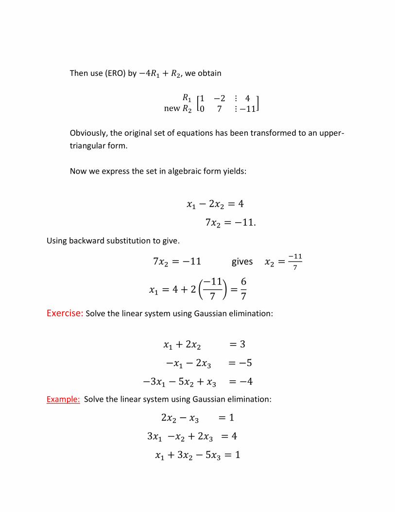
Then use (ERO) by −4𝑅1 + 𝑅2, we obtain

𝑅1

new 𝑅2 [

1 −2 ⋮0 7 ⋮

4

−11]

Obviously, the original set of equations has been transformed to an upper-

triangular form.

Now we express the set in algebraic form yields:

𝑥1 − 2𝑥2 = 4

7𝑥2 = −11.

Using backward substitution to give.

7𝑥2 = −11 gives 𝑥2 =−11

7

𝑥1 = 4 + 2 (−11

7) =

6

7

Exercise: Solve the linear system using Gaussian elimination:

𝑥1 + 2𝑥2 = 3

−𝑥1 − 2𝑥3 = −5

−3𝑥1 − 5𝑥2 + 𝑥3 = −4

Example: Solve the linear system using Gaussian elimination:

2𝑥2 − 𝑥3 = 1

3𝑥1 −𝑥2 + 2𝑥3 = 4

𝑥1 + 3𝑥2 − 5𝑥3 = 1

Solution: The augmented matrix form of the system given by

[0 2 −1 ⋮ 13 −1 2 ⋮ 41 3 −5 ⋮ 1

]

Note: To solve this system, the Gaussian elimination method will fail immediately because the element in the first row on the leading diagonal, (the pivot) is zero. Thus, it is impossible to divide that row by the pivot value. Clearly this difficulty can be overcome by rearranging the order of the row.

For example, we making the first row the third, we obtain

[1 3 −5 ⋮ 13 −1 2 ⋮ 40 2 −1 ⋮ 1

]

Now we can use the usual elimination process. The first elimination step is to

eliminate the element 𝑎21from the second row by adding a −3 multiple of row one (−3𝑅1 + 𝑅2), which give

[1 3 −5 ⋮ 10 −10 17 ⋮ 10 2 −1 ⋮ 1

]

We finish with first elimination step. Since the element 𝑎31 is already zero .

The second elimination step is to eliminate the element 𝑎32from the third row by

adding a 2

10 multiple of row two (

2

10𝑅2 + 𝑅3), which give

[

1 3 −5 ⋮ 10 −10 17 ⋮ 1

0 012

5 ⋮

6

5

]

Obviously, the original set of equations has been transformed to an upper-

triangular form.

Now we express the set in algebraic form yields:

𝑥1 + 3𝑥2 − 5𝑥3 = 1

−10𝑥2 + 17𝑥3 = 1

12

5𝑥3 =

6

5

Using backward substitution to give.

12

5𝑥3 =

6

5 gives 𝑥3=

1

2

−10𝑥2 + 17(1

2)= 1 gives 𝑥2=

3

4

𝑥1 + 3 (3

4) − 5 (

1

2 ) = 1 gives 𝑥1=

5

4

Example: Solve the linear system using Gaussian elimination:

2𝑥1 + 2𝑥2 − 4𝑥3 = 0

2𝑥1 +2𝑥2−𝑥3 = 1

3𝑥1 + 2𝑥2 − 3𝑥3 = 3

Solution : The augmented matrix form of the system given by

[2 2 −4 ⋮ 02 2 −1 ⋮ 13 2 −3 ⋮ 3

]

The first elimination step is to eliminate the element 𝑎21from the second row by

adding a −1 multiple of row one (−𝑅1 + 𝑅2) and the element 𝑎31from the

thired row by adding a −3

2 multiple of row one (−

3

2 𝑅1 + 𝑅3), which give

[2 2 −4 ⋮ 00 0 3 ⋮ 10 −1 3 ⋮ 3

]

We finish with first elimination step.

To start second elimination step is to eliminate the element 𝑎22from the second row which is zero ( is called second pivot element), the Gaussian elimination method cannot continue in its present form .

Therefore, we interchange row two and row three to obtain

[2 2 −4 ⋮ 00 −1 3 ⋮ 30 0 3 ⋮ 1

]

We finish with the second elimination step. Since the element 𝑎32 is already zero .

Then obviously, the original set of equations has been transformed to an upper-

triangular form. Now we express the set in algebraic form yields:

2𝑥1 + 2𝑥2 − 4𝑥3 = 0

−𝑥2 + 3𝑥3 = 3

3𝑥3 = 1

Using backward substitution to give.

3𝑥3 = 1 gives 𝑥3=1

3

−𝑥2 + 3(1

3)= 3 gives 𝑥2=−2

2𝑥1 + 2(−2) − 4 (1

3 ) = 0 gives 𝑥1=

8

3

Pivoting strategies : In the previous part we discussed Gaussian elimination and Gaussian elimination was applied to a problem with no pivotal elements zero.

However, the method did not work

if the first coefficient of the first equation or

if a diagonal coefficient become zero in the process of the solution because they are used as denominator in the forward elimination.

Then pivoting is used to change sequential order of the equation for two purposes

1- To prevent diagonal coefficients form becoming zero. 2- To make each diagonal coefficient larger in value (magnitude) than any

other coefficient below it. That is to decrease the round-off errors.

1- Partial Pivoting(or row Pivoting) the basic approach is to use the largest ( in absolute value ) element on or below the diagonal in the column of current interest as the pivotal element for elimination in the rest of that column.

One immediate effort of this will be to force all the multiples used to be not grater than (1) in absolute.

Example : Solve the linear system using Gaussian elimination with partial pivoting:

2𝑥1 + 2𝑥2 − 2𝑥3 = 8

−4𝑥1 −2𝑥2+2𝑥3 = −14

−2𝑥1 + 3𝑥2 + 9𝑥3 = 9

Solution : For the first elimination step, since −4 is the largest absolute coefficient

of first variable 𝑥1. Then we need to interchange, the first row and the second

row, give us

−4𝑥1 −2𝑥2+2𝑥3 = −14

2𝑥1 + 2𝑥2 − 2𝑥3 = 8

−2𝑥1 + 3𝑥2 + 9𝑥3 = 9

The first elimination step is to eliminate the element 𝑎21from the second row by

adding a 2

4 multiple of row one (

2

4𝑅1 + 𝑅2) and the element 𝑎31from the thired

row by adding a −2

4 multiple of row one (−

2

4 𝑅1 + 𝑅3), which give

−4𝑥1 −2𝑥2+2𝑥3 = −14

𝑥2 − 2𝑥3 = 1

4𝑥2 + 8𝑥3 = 16

We finish with first elimination step. For second elimination step (4) is the largest absolute coefficient of the second variablex2. Then we need to interchange, the second row and the third row, give us

−4𝑥1 −2𝑥2+2𝑥3 = −14

4𝑥2 + 8𝑥3 = 16

𝑥2 − 𝑥3 = 1

Eliminate the second variable 𝑥2 (element 𝑎32) from the third row by adding a −1

4

multiple of row two ( −1

4𝑅2 + 𝑅3) , which give

−4𝑥1 −2𝑥2+2𝑥3 = −14

4𝑥2 + 8𝑥3 = 16

−3𝑥3 = −3

Then obviously, the original set of equations has been transformed to an upper-

triangular form. Using backward substitution give.

3𝑥3 = −3 Gives 𝑥3=1, 𝑥2=2 and 𝑥1=3.

2- Total Pivoting : In the case total pivoting ( or complete pivoting ), we search

for the largest number( in absolute value ) in the entire array instead of just

in the first column and this number is the pivot, This means that we shall

probably need to interchange the column as well as rows.

Example : Solve the linear system using Gaussian elimination with total pivoting:

2𝑥1 + 2𝑥2 − 2𝑥3 = 8

−4𝑥1 −2𝑥2+2𝑥3 = −14

−2𝑥1 + 3𝑥2 + 9𝑥3 = 9

Solution : For the first elimination step, since 9 is the largest absolute coefficient of

first variable 𝑥3 in the given system. Then we need to interchange, the first row

and the third row as well as the first column and the third column, give us

9𝑥3 +3𝑥2−2𝑥1 = 9

2𝑥3 − 2𝑥2 − 4𝑥1 = −14

−2𝑥3 + 2𝑥2 + 2𝑥1 = 8

The first elimination step is to eliminate the third variable 𝑥3 from the second row

by adding a −2

9 multiple of row one ( −

2

9 𝑅1 + 𝑅2) and the third row by adding a

2

9 multiple of row one (

2

9 𝑅1 + 𝑅3), which give

9𝑥3 +3𝑥2−2𝑥1 = 9

−8

3𝑥2 −

32

9𝑥1 = −16

8

3𝑥2 +

14

9𝑥1 = 10

We finish with first elimination step. For second elimination step (−32

9) is the

largest absolute coefficient of the second variable x1. Then we need to interchange, the second row and the third row as well as the second column and the third column, give us

9𝑥3 −2𝑥1 + 3𝑥2 = 9

−32

9𝑥1 −

8

3𝑥2 = −16

14

9𝑥1 +

8

3𝑥2 = 10

Eliminate the first variable 𝑥1 from the third row by adding −7

16 multiple of row

two ( −7

16𝑅2 + 𝑅3) , which give

9𝑥3 −2𝑥1 + 3𝑥2 = 9

−32

9𝑥1 −

8

3𝑥2 = −16

3

2𝑥2 = 10

Then obviously, the original set of equations has been transformed to an upper-

triangular form. Using backward substitution give

3

2𝑥2 = 10 Gives 𝑥2=2, 𝑥1=3 and 𝑥3=1.

Ex:

1- Solve the linear system using Gaussian elimination with partial pivoting.

𝑥1 − 𝑥2 + 3𝑥3 = 13

4𝑥1 − 2𝑥2 + 𝑥3 = 15

− 3𝑥1 − 𝑥2 + 4𝑥3 = 8

𝑥1 = 2 , 𝑥2 = −2, 𝑥3=3.

2- Solve the linear system using Gaussian elimination with total pivoting.

𝑥1 + 𝑥2 − 𝑥3 = −3

2𝑥1 − 3𝑥2 + 4𝑥3 = 23

− 3𝑥1 + 𝑥2 − 𝑥3 = −15

𝑥1 = 2 , 𝑥2 = −1, 𝑥3=4.

Write your solution process as augmented matrix.

4- GAUSSIAN – Jordan method: This method is a modification of the

Gaussian elimination method. The Gauss-Jordan method, however, is

inefficient for practical calculation, but is often useful for theoretical

purposes. The basis of this method is to convert the given matrix into

diagonal form. The forward elimination of the Gauss-Jordan method is

identical to that of the Gaussian elimination method.

However, Gauss-Jordan method uses backward elimination rather than

backward substitution. In the Gauss-Jordan method the forward elimination

and backward elimination not need to separate.

This is possible because a pivot element can be used to eliminate the

coefficient not only in below but also above at same time. If this approach is

taken, the form of this coefficient matrix becomes diagonal.

Example: Solve the linear system using GAUSSIAN – Jordan method:

𝑥1 + 2𝑥2 = 3

−𝑥1 −2𝑥3 = −5

−3𝑥1 − 5𝑥2 + 𝑥3 = −4

Solution : The augmented matrix form of the system given by

[1 2 0 ⋮ 3

−1 0 −2 ⋮ −5−3 −5 1 ⋮ −4

]

The first elimination step is to eliminate the element 𝑎21 by adding row one and

row two (𝑅1 + 𝑅2) and the element 𝑎31 by adding a 3multiple of row one and row three (3𝑅1 + 𝑅3), which give

[1 2 0 ⋮ 30 2 −2 ⋮ −20 1 1 ⋮ 5

]

We finish with first elimination step. The second row is now divided by (2) to give

[1 2 0 ⋮ 30 1 −1 ⋮ −10 1 1 ⋮ 5

]

To start second elimination step is to eliminate the element 𝑎12 by adding

(−2) multiple row two and row one (−2𝑅2 + 𝑅1) and the element 𝑎32 by

subtract row two and row three (𝑅1−𝑅3), which give

[1 0 2 ⋮ 50 1 −1 ⋮ −10 0 2 ⋮ 6

]

The third row is now divided by (2) to give

[1 0 2 ⋮ 50 1 −1 ⋮ −10 0 1 ⋮ 3

]

The third elimination step is to eliminate the element 𝑎23 by adding row three

and row two (𝑅3 + 𝑅2) and the element 𝑎13 by adding (−2) multiple of row three and row one (−2𝑅3+𝑅1), which give .

[1 0 0 ⋮ −10 1 0 ⋮ 20 0 1 ⋮ 3

]

Obviously, the original set of equations has been transformed to an upper-

triangular form yields:

𝑥1=−1 , 𝑥2=2 and 𝑥3=3.

Ex: Solve the linear system using Gaussian – Jordan method

𝑥1 + 𝑥2 + 𝑥3 = −3

2𝑥1 + 3𝑥2 + 7𝑥3 = 0

𝑥1 + 3𝑥2 − 2𝑥3 = 17

𝑥1 = 1 , 𝑥2 = 4, 𝑥3=-2.

Ex:

1- Ali and Layla both entered a quiz. The quiz had twenty questions and points

were allocated as follows:

• x points were added for each correctly answered question.

• y points were deducted for each incorrect (or unanswered) question.

Ali got 15 questions correct and scored 65 points.

Layla got 11 questions correct and scored 37 points.

Use matrices to find the value of x and y.

2- A store sells flash memory and CD's. All the flash memory have the same price

and all the CD's have the same price.

Dana and Sara both shopped at the store.

Dana bought 5 flash memories and 3 CD's and paid altogether $90

Sara bought 2 flash memories and 8 CD's and paid altogether $138

Use matrices to find the cost of one flash memory and one CD.