chapter 025
TRANSCRIPT

1Copyright © 2013, 2009, 2005, 2001, 1997 by Saunders, an imprint of Elsevier Inc.
Chapter 25
Using Statistics to Determine Differences

2Copyright © 2013, 2009, 2005, 2001, 1997 by Saunders, an imprint of Elsevier Inc.
Using Statistics to Determine Differences
Differences among groups Different tests for data at the various levels of
measurement Parametric statistics (used with normally
distributed interval-level and ratio-level data): Independent samples t-test Paired t-test ANOVA

3Copyright © 2013, 2009, 2005, 2001, 1997 by Saunders, an imprint of Elsevier Inc.
Using Statistics to Determine Differences (Cont’d)
Nonparametric statistics (used with non-normally distributed samples and with ordinal-level and nominal-level data): Mann-Whitney U Wilcoxon signed-ranks test Kruskal-Wallis H Chi-square test of independence (Nominal data
only)

4Copyright © 2013, 2009, 2005, 2001, 1997 by Saunders, an imprint of Elsevier Inc.
Choosing Parametric Versus Nonparametric Statistics to Determine Differences
Parametric statistics are always associated with a certain set of assumptions that the data must meet
One of these is normal distribution—perform a test of normalcy on the data K² test Shapiro-Wilk test Kolmogorov-Smirnov D test

5Copyright © 2013, 2009, 2005, 2001, 1997 by Saunders, an imprint of Elsevier Inc.
t-Tests
Independent t-test—examines difference between two independent groups
Paired (dependent) t-test—examines differences between two matched or paired groups or a comparison of pre-and post-test measurements

6Copyright © 2013, 2009, 2005, 2001, 1997 by Saunders, an imprint of Elsevier Inc.
t-Test for Independent Samples
Samples are independent if study participants in one group are unrelated or different than those in second group
Groups are independent if study subjects are randomly assigned to either treatment or control group and are not matched on any variables
Often used to measure the difference in two similar groups After intervention

7Copyright © 2013, 2009, 2005, 2001, 1997 by Saunders, an imprint of Elsevier Inc.
t-Test for Independent Samples (Cont’d)
Most common parametric analysis technique used in nursing
Assumptions: Normal distribution Dependent variable measured at the interval/ratio
level Equal variance, both samples All observations independent

8Copyright © 2013, 2009, 2005, 2001, 1997 by Saunders, an imprint of Elsevier Inc.
t-Test for Independent Samples (Cont’d)
Formula:
where: = mean of group 1 = mean of group 2 = the standard error of the difference
between the two groups

9Copyright © 2013, 2009, 2005, 2001, 1997 by Saunders, an imprint of Elsevier Inc.
t-Test for Independent Samples (Cont’d)
If the two groups have different sample sizes, then use this formula for the denominator:
where n1 = group 1 sample size
n2 = group 2 sample size
s1 = group 1 variance
s2 = group 2 variance

10Copyright © 2013, 2009, 2005, 2001, 1997 by Saunders, an imprint of Elsevier Inc.
t-Test for Independent Samples (Cont’d)
If the two groups have the same number of subjects in each group, then one can use this simplified formula for the denominator:
where n = the sample size in each group and not the
total sample of both groups
11Copyright © 2013, 2009, 2005, 2001, 1997 by Saunders, an imprint of Elsevier Inc.
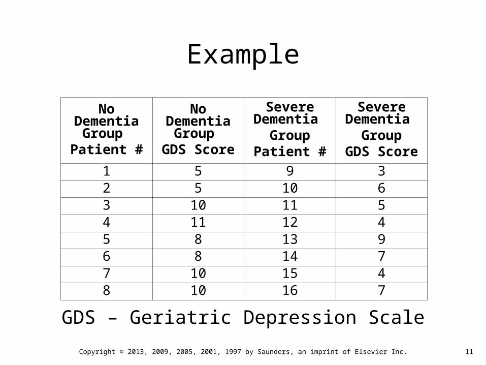
Example
GDS – Geriatric Depression Scale
No Dementia Group
Patient #
No Dementia Group
GDS Score
Severe Dementia
GroupPatient #
Severe Dementia
GroupGDS Score
1 5 9 32 5 10 63 10 11 54 11 12 45 8 13 96 8 14 77 10 15 48 10 16 7

12Copyright © 2013, 2009, 2005, 2001, 1997 by Saunders, an imprint of Elsevier Inc.
Example (Cont’d)
The independent variable level of dementia no dementia severe dementia
Dependent variable—score on the Geriatric Depression Scale
Null hypothesis is: There are no significant differences between those with dementia and those without dementia on depression scores

13Copyright © 2013, 2009, 2005, 2001, 1997 by Saunders, an imprint of Elsevier Inc.
Example Computations for the t-Test
Step 1: Compute means for both groups, which involves the sum of scores for each group divided by the number in the group
The mean for Group 1, No Dementia:
The mean for Group 2, Severe Dementia:

14Copyright © 2013, 2009, 2005, 2001, 1997 by Saunders, an imprint of Elsevier Inc.
Example Computations for the t-Test (Cont’d)
Step 2: Compute the numerator of the t-test:

15Copyright © 2013, 2009, 2005, 2001, 1997 by Saunders, an imprint of Elsevier Inc.
Example Computations for the t-Test
Step 3: Compute the standard error of the difference compute the variances for each group
• s2 for Group 1 = 5.41
• s2 for Group 2 = 3.98 Plug into the standard error of the difference formula

16Copyright © 2013, 2009, 2005, 2001, 1997 by Saunders, an imprint of Elsevier Inc.
Example Computations for the t-Test (Cont’d)
Step 4: Compute t value:

17Copyright © 2013, 2009, 2005, 2001, 1997 by Saunders, an imprint of Elsevier Inc.
Example Computations for the t-Test (Cont’d)
Step 5: Compute your degrees of freedom:
df = n1+ n2 – 2
df = 8 + 8 – 2
df = 14

18Copyright © 2013, 2009, 2005, 2001, 1997 by Saunders, an imprint of Elsevier Inc.
Example Computations for the t-Test (Cont’d)
Locate the critical t value in the t distribution table and compare to the obtained t value
The critical t value for 14 degrees of freedom at alpha (α) = 0.05 is 2.15
if calculated t is between –2.15 and +2.15, researcher must accept the null hypothesis
If calculated t is Less than –2.15, or More than +2.15, researcher would Reject null hypothesis

19Copyright © 2013, 2009, 2005, 2001, 1997 by Saunders, an imprint of Elsevier Inc.
Example Interpretation of Results
t is 2.55, and it is Greater Than the critical value of 2.15. This means that the researcher will Reject the null hypothesis.

20Copyright © 2013, 2009, 2005, 2001, 1997 by Saunders, an imprint of Elsevier Inc.
Example Interpretation of Results (Cont’d)
In the research report, the researcher’s statement would be: An independent samples t-test computed on GDS scores revealed long-term residents with no dementia had significantly higher depression scores than did those who had severe dementia, t(14) = 2.55, p < 0.05; = 8.4 versus 5.6, respectively

21Copyright © 2013, 2009, 2005, 2001, 1997 by Saunders, an imprint of Elsevier Inc.
Example Interpretation of Results (Cont’d)
“t(14) = 2.55” means that a t-test was used, that the degrees of freedom were 14, and that the calculated value was 2.55
p < .005 means that the value of 2.55 obtained was so unusually high that instead of the p-value of < .05, which means that the results have a 5% chance (1 in 20) of being due to Type I error, the results have only a 0.5% chance (1 in 200) of being due to Type I error. The results are very, very convincing.

22Copyright © 2013, 2009, 2005, 2001, 1997 by Saunders, an imprint of Elsevier Inc.
Non-Parametric Alternative
Mann-Whitney U test Difference between rankings of members of
both groups Often used to measure difference in two
similar groups After intervention

23Copyright © 2013, 2009, 2005, 2001, 1997 by Saunders, an imprint of Elsevier Inc.
Non-Parametric Alternative (Cont’d)
Very commonly used in nursing Assumptions:
Distribution may be normal or non-normal Dependent variable measured at interval/ratio or
ordinal level

24Copyright © 2013, 2009, 2005, 2001, 1997 by Saunders, an imprint of Elsevier Inc.
t-Tests for Paired Samples
Assumptions Differences between the paired scores are
independent Normally or approximately normal distribution Dependent variable measured at the interval/ratio
level
25Copyright © 2013, 2009, 2005, 2001, 1997 by Saunders, an imprint of Elsevier Inc.
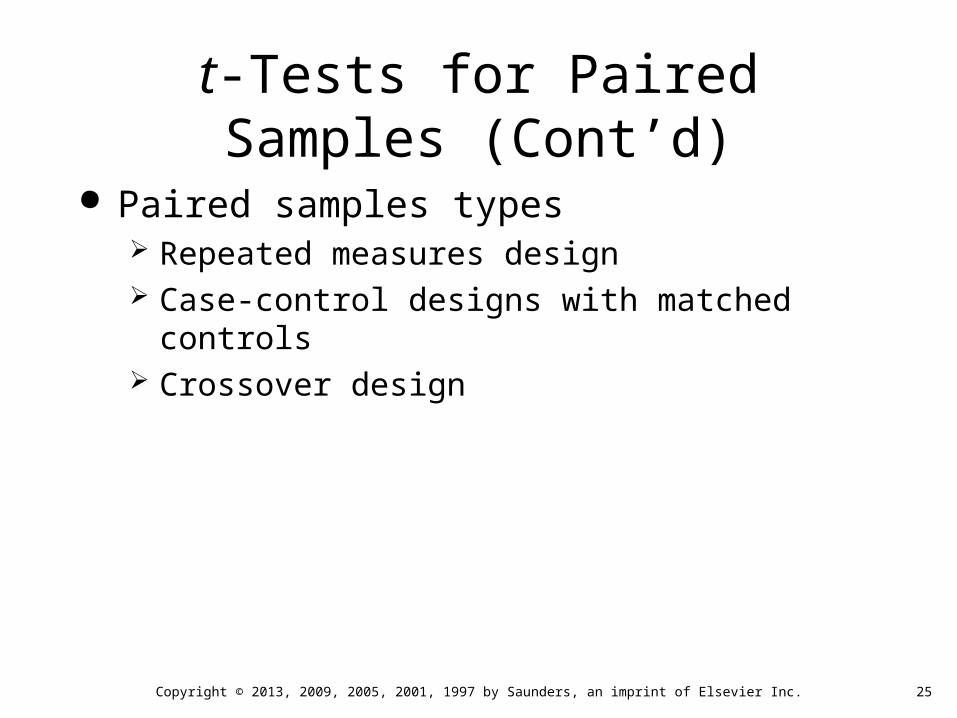
t-Tests for Paired Samples (Cont’d)
Paired samples types Repeated measures design Case-control designs with matched controls Crossover design

26Copyright © 2013, 2009, 2005, 2001, 1997 by Saunders, an imprint of Elsevier Inc.
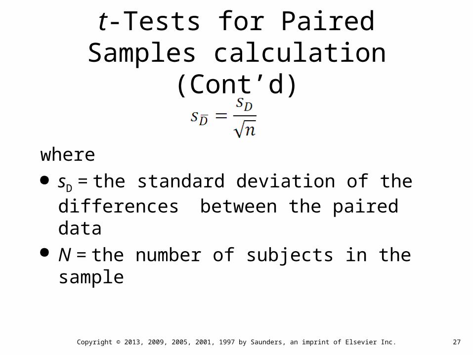
t-Tests for Paired Samples calculation
where = the mean difference of the paired data = the standard error of the difference
27Copyright © 2013, 2009, 2005, 2001, 1997 by Saunders, an imprint of Elsevier Inc.
t-Tests for Paired Samples calculation (Cont’d)
where sD = the standard deviation of the differences
between the paired data N = the number of subjects in the sample

28Copyright © 2013, 2009, 2005, 2001, 1997 by Saunders, an imprint of Elsevier Inc.
Example
Level of functional impairment among 10 adults receiving rehabilitation for a painful injury
Independent variable: treatment over time (three weeks of rehab)
Dependent variable: functional impairment (measured twice) (lower score is healthier)
Null hypothesis is: There is no significant reduction in functional impairment from baseline to post-treatment for patients in a rehabilitation program

29Copyright © 2013, 2009, 2005, 2001, 1997 by Saunders, an imprint of Elsevier Inc.
Example (Cont’d)
Functional Impairment Levels at Baseline and Post-Treatment
Subject #
Baseline FunctionalImpairment
Scores
Post-Treatment Functional
Impairment Scores Difference
1 2.9 1.7 1.22 5.7 2.9 2.83 2.3 2.9 –0.64 3.9 3 0.95 3.8 3.1 0.76 3.3 3.2 0.17 2.9 3.2 –0.38 4.7 3.2 1.59 3.2 2.1 1.1
10 4.9 3.4 1.5

30Copyright © 2013, 2009, 2005, 2001, 1997 by Saunders, an imprint of Elsevier Inc.
Example t-Test Computations
Step 1: Compute difference between each subject's data pair (see last column of Table)
Step 2: Compute mean of the difference scores, which becomes the numerator of the t-test:

31Copyright © 2013, 2009, 2005, 2001, 1997 by Saunders, an imprint of Elsevier Inc.
Example t-Test Computations (Cont’d)
Step 3: Compute the standard error of the difference Compute the standard deviation of the difference scores
S = 0.99 Plug into the standard error of the difference formula

32Copyright © 2013, 2009, 2005, 2001, 1997 by Saunders, an imprint of Elsevier Inc.
Example t-Test Computations (Cont’d)
Step 4: Compute t value:

33Copyright © 2013, 2009, 2005, 2001, 1997 by Saunders, an imprint of Elsevier Inc.
Example t-Test Computations (Cont’d)
Step 5: Compute degrees of freedom:
df = n –1
df = 10 –1
df = 9

34Copyright © 2013, 2009, 2005, 2001, 1997 by Saunders, an imprint of Elsevier Inc.
Example t-Test Computations (Cont’d)
Step 6: Locate critical t value on the t distribution table and compare to the obtained t value
The critical t value for 9 degrees of freedom at alpha (α) = 0.05 is 2.26. If calculated t is between –2.26 and +2.26,
researcher must Accept the null hypothesis If calculated t is Less than –2.26, or More than
+2.26 researcher would Reject the null hypothesis

35Copyright © 2013, 2009, 2005, 2001, 1997 by Saunders, an imprint of Elsevier Inc.
Example Interpretation of Results
The obtained t is 2.84, which is Greater Than the critical value of 2.26. This means that the researcher will Reject the null hypothesis
Thus during the three-week rehabilitation program, patients successfully reduced their functional impairment levels

36Copyright © 2013, 2009, 2005, 2001, 1997 by Saunders, an imprint of Elsevier Inc.
Example Interpretation of Results (Cont’d)
In the research report, the researcher’s statement would be: A paired samples t-test computed on MPI functional impairment scores revealed that the patients undergoing rehabilitation had significantly lower functional impairment levels from baseline to post-treatment, t(9) = 2.84, p < 0.05; = 3.8 versus 2.9, respectively.

37Copyright © 2013, 2009, 2005, 2001, 1997 by Saunders, an imprint of Elsevier Inc.
Non-parametric Alternative
Wilcoxon signed-rank test The difference between the rankings of the
members of both groups Often used to measure the difference in two
similar groups After intervention A very common nonparametric analysis
technique used in nursing
38Copyright © 2013, 2009, 2005, 2001, 1997 by Saunders, an imprint of Elsevier Inc.
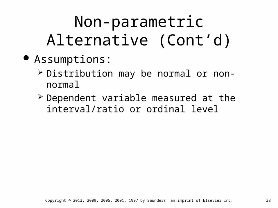
Non-parametric Alternative (Cont’d)
Assumptions: Distribution may be normal or non-normal Dependent variable measured at the interval/ratio
or ordinal level

39Copyright © 2013, 2009, 2005, 2001, 1997 by Saunders, an imprint of Elsevier Inc.
One-way Analysis of Variance (ANOVA)
Statistical procedure that compares data between two or more groups or conditions
(Rarely used for two groups—t-test is more common with two)
Purpose: to investigate the presence of differences between those groups
Dependent variable continuous (interval or ratio)
Computes two estimates of variance—between and among

40Copyright © 2013, 2009, 2005, 2001, 1997 by Saunders, an imprint of Elsevier Inc.
One-way Analysis of Variance (Cont’d)
Produces the F statistic
Mean Square = Variance This value is compared with values in an F
distribution table, to determine whether the groups’ dependent variables differ significantly from one another

41Copyright © 2013, 2009, 2005, 2001, 1997 by Saunders, an imprint of Elsevier Inc.
Example
Medical costs among 15 females receiving treatment for a chronic pain condition, monthly medical costs for one year incurred after treatment ended were examined
Independent variable—type of treatment or intervention
Dependent variable—average medical costs incurred per month
Null hypothesis: There is no significant difference between the treatment groups on post-treatment monthly medical costs

42Copyright © 2013, 2009, 2005, 2001, 1997 by Saunders, an imprint of Elsevier Inc.
Example (Cont’d)
Costs were U.S. Dollars, averaged monthly
Multidisciplinary Group Costs
Standard Care
Group CostsPharmacotherapy
Group Costs
74 168 603
748 328 707
433 186 868
422 199 286
297 154 919
Total 1974 1035 3383
Grand Total (G) = 6392

43Copyright © 2013, 2009, 2005, 2001, 1997 by Saunders, an imprint of Elsevier Inc.
Example (Cont’d)
Step 1: Compute correction term, C Square the grand sum (G), and divide by total N
Step 2: Compute Total Sum of Squares Square every value in dataset, sum, and subtract
C
742 + 7482 + + 9192 – 2723844.3 = 1071877.7

44Copyright © 2013, 2009, 2005, 2001, 1997 by Saunders, an imprint of Elsevier Inc.
Example (Cont’d)
Step 3: Compute Between Groups Sum of Squares Square the sum of each column and divide by N. Add each, and then subtract C
(779335.2 + 214245 + 2288937.8) – 2723844.3
= 558673.7

45Copyright © 2013, 2009, 2005, 2001, 1997 by Saunders, an imprint of Elsevier Inc.
Example (Cont’d)
Step 4: Compute within Groups Sum of Squares Subtract the Between Groups Sum of Squares
(Step 3) from Total Sum of Squares (Step 2) 1071877.7 – 558673.7 = 513204
Calculate the degrees of freedom (df) Mean square between groups df = number of groups – 1 Mean square within groups df =(number of groups –1) (n–1)

46Copyright © 2013, 2009, 2005, 2001, 1997 by Saunders, an imprint of Elsevier Inc.
Example (Cont’d)
Step 5: Calculate F by dividing the MS between by the MS within
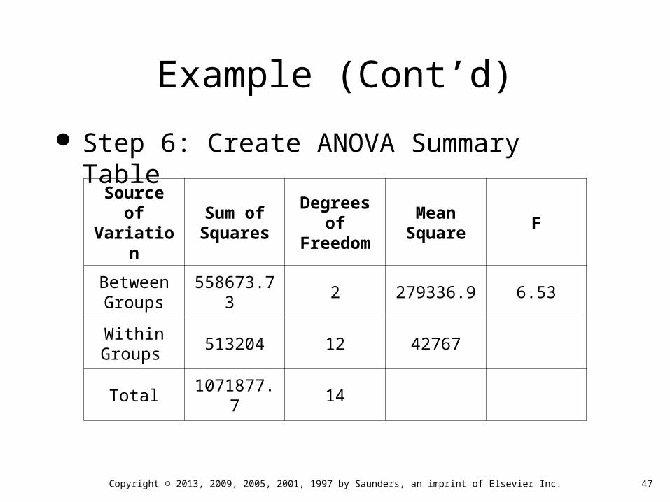
47Copyright © 2013, 2009, 2005, 2001, 1997 by Saunders, an imprint of Elsevier Inc.
Example (Cont’d)
Step 6: Create ANOVA Summary Table
Source of Variation
Sum of Squares
Degrees of Freedom
Mean Square
F
Between Groups
558673.73 2 279336.9 6.53
Within Groups
513204 12 42767
Total 1071877.7 14

48Copyright © 2013, 2009, 2005, 2001, 1997 by Saunders, an imprint of Elsevier Inc.
Example (Cont’d)
Step 7: Locate the critical F value on the F distribution table and compare to our obtained F value with it. The critical F value for 2 and 12 degrees of
freedom at alpha (α) = 0.05 is 3.88. Our obtained F is 6.53, which exceeds the critical value

49Copyright © 2013, 2009, 2005, 2001, 1997 by Saunders, an imprint of Elsevier Inc.
Example Interpretation of Results
The obtained F= 6.53 exceeds the critical value in the table, which means that the F is statistically significant and that the population means are not equal. Therefore, the researcher rejects the null hypothesis that the three groups have the same monthly post-treatment medical costs.

50Copyright © 2013, 2009, 2005, 2001, 1997 by Saunders, an imprint of Elsevier Inc.
Example Interpretation of Results (Cont’d)
However, the F does not reveal which treatment groups differ from one another. Further testing, termed multiple comparison tests or post-hoc tests, are required to complete the ANOVA process and determine all the significant differences among the study groups

51Copyright © 2013, 2009, 2005, 2001, 1997 by Saunders, an imprint of Elsevier Inc.
Post Hoc Tests
Developed specifically to determine the location of group differences after ANOVA is performed on data from more than two groups
Frequently used post hoc tests Newman-Keuls test Tukey Honestly Significant Difference (HSD) test Scheffé test Dunnett test

52Copyright © 2013, 2009, 2005, 2001, 1997 by Saunders, an imprint of Elsevier Inc.
Post Hoc Tests (Cont’d)
All divide the alpha (usually p < .05) over all groups
After Tukey HSD testing was computed for the example: Pharmacotherapy group and Standard care group
costs were significantly different (Pharm group costs higher by a wide margin)

53Copyright © 2013, 2009, 2005, 2001, 1997 by Saunders, an imprint of Elsevier Inc.
Non-parametric Alternative
Kruskal-Wallis test Dependent variable may be ordinal Data converted to ranks, which are then
compared Used for answering the question, “Are these
all the same?”

54Copyright © 2013, 2009, 2005, 2001, 1997 by Saunders, an imprint of Elsevier Inc.
Other ANOVA Procedures
Randomized complete block Repeated measures Factorial

55Copyright © 2013, 2009, 2005, 2001, 1997 by Saunders, an imprint of Elsevier Inc.
Chi-square Test of Independence
Compares differences in proportions (percentages) of nominal level variables
One-way chi-square: compares different levels of one variable only
Two-way chi-square: tests whether proportions in levels of one variable are significantly different from proportions of the second variable

56Copyright © 2013, 2009, 2005, 2001, 1997 by Saunders, an imprint of Elsevier Inc.
Assumptions of the Chi-Square Test
One data point for each subject (no repeated measures)
Mutually exclusive categories Mutually exhaustive categories Distribution-free, or nonparametric—no
requirement of normal distribution

57Copyright © 2013, 2009, 2005, 2001, 1997 by Saunders, an imprint of Elsevier Inc.
Formula (Two-way Chi-Square)
where the Contingency table is labeled as such:
A B
C D

58Copyright © 2013, 2009, 2005, 2001, 1997 by Saunders, an imprint of Elsevier Inc.
Example (Two-way Chi-Square)
Presence of candiduria among 97 adults with a spinal cord injury
Candiduria
Antibiotic Use
Yes No
Yes 15 43
No 0 39

59Copyright © 2013, 2009, 2005, 2001, 1997 by Saunders, an imprint of Elsevier Inc.
Calculation

60Copyright © 2013, 2009, 2005, 2001, 1997 by Saunders, an imprint of Elsevier Inc.
Degrees of Freedom (df)
Must be calculated to determine the significance of the value of the statistic
df = (R –1)(C – 1)
where R = Number of rows C = Number of columns
df = (2 –1)(2 –1) = 1

61Copyright © 2013, 2009, 2005, 2001, 1997 by Saunders, an imprint of Elsevier Inc.
Interpretation of Results
The chi-square statistic is compared with the chi-square values in the table in Appendix X. The table includes the critical values of chi-square for specific degrees of freedom at selected levels of significance. If the value of the statistic is equal to or greater than the value identified in the chi-square table, the difference between the two variables is statistically significant.

62Copyright © 2013, 2009, 2005, 2001, 1997 by Saunders, an imprint of Elsevier Inc.
Interpretation of Results (Cont’d)
The critical 2 for df = 1 is 3.84, and the researcher’s obtained 2 is 11.93, thereby exceeding the critical value and indicating a significant difference between antibiotic users and non-users on the presence of candiduria.

63Copyright © 2013, 2009, 2005, 2001, 1997 by Saunders, an imprint of Elsevier Inc.
Interpretation of Results (Cont’d)
A research report would read: Antibiotic users had significantly higher rates of candiduria than those who did not use antibiotics (26% versus 0%, respectively). This finding suggests that antibiotic use may be a risk factor for developing candiduria, and further research is needed to investigate candiduria as a direct effect of antibiotics.