1

Chapter 1

Introduction

The subject of this text is the shell of revolution. The first question may be: just what is a shell? A mathematical definition is in the next chapter, but for the moment, a shell may be considered as a structural element, one dimension of which is "thin", and which has curvature. The curvature has a very significant effect on the behavior of a structure in carrying loads. §1.1 Effect of Curvature The most widely used structural element is the straight beam. The key feature which must be considered in any design is the type of load which the beam carries. In Fig. 1 a basic structural principle is indicated. A beam is shown which has a tangential (axial) load N which causes the axial displacement u, and in the lower part of the figure has a transverse load Q which causes the displacement w. The stiffness and maximum stress in the former case, which can be obtained from elementary considerations, are

Nu =

E tL σmax =

Νt (1.1)

in which E is the elastic modulus (Young's modulus) and the load is force per unit of width. In the case of the transverse load, the stiffness and maximum stress are

Qw = E tL

t2

4 L2σmax =

Qt

6 Lt

(1.2) From a comparison of (1.1) and (1.2) it is seen that for a slender beam with, say, L/t = 10, the stiffness is less by a factor of 400, and the stress is higher by a factor of 60 for the latter case of transverse load. So for efficient load carrying, it is highly desirable to have only axial loads. There are, of course, situations in which a high degree of flexibility of the structure is important, and the loading should be transverse.

L

t

Q, w

N, u

2

Figure 1.1 - Flat beam or plate with two types of load. The basic structural principle is that the stiffness and load-carrying capability is much greater for tangential loads (a) than for transverse loads (b).

The simple principle of using only tension and compression elements for structural efficiency is not practical in many situations. For one example, it comes in conflict with irrepressible human urge to span space. Fig. 1.2 is a sketch of a Greek temple construction. Although timber construction was used for the main parts of the roof, the facade is stone. No mortar has yet been invented which would make possible a beam consisting of stone segments capable of carrying its own weight. For stone construction, of course, the problem is not the stress magnitude, but that the mortar cannot sustain the significant tensile portion of the bending stress which is caused by the transverse load in Fig. 1.1. Thus a severe restriction is placed on the distance between supporting columns.

Figure 1.2 - Greek temple. The result is beautiful but massive, due to the restriction on the maximum length of the stone roof elements.

An attempt to solve the restriction on the free space with a masonry construction is the "corbeled arch" indicated in Fig. 1.3. It is not difficult to understand why this was not widely used. Any small shift in the foundation settlement or in the loading could cause severe problems.

3

Figure 1.3 - Corbeled arch. From 4000 BC, the Egyptians attempted to span space with this somewhat unreliable construction method.

The true arch construction is shown in Fig. 1.4. In contrast to the corbeled arch, in which space is spanned, but in a manner which is structurally unsound, the true arch utilizes the shape of the space for structural efficiency. In terms of Fig. 1.1, one may say that the arches in Fig. 1.4 convert the applied transverse load into a compressive load between the elements because of the curvature and because of the shape of the elements. The Romans utilized the arch for both imposing civic structures, such as the coliseum, and quite utilitarian structures as the underground sewer system and the aqueducts. The aqueduct over the Neva River, built under Trajan in 105AD, is about 30 meters high and has a distance between support points of about 33 meters. Many of these aqueducts built all across Europe stand today, nearly 2000 years later, without the help of any mortar at all. The arch in Fig. 1.4a was the basis for the cathedral construction of the 12th century AD referred to as Roman. At the end of the 12th century, the transition was made to the Gothic style of construction which utilizes extensively the pointed arch Fig. 1.4b, as well as the "flying buttress", which provides the means for carrying the lateral loads when the arch is made more shallow than shown in Fig. 1.4. The remarkable past and present structural creations are representative of human ingenuity and creativity. As we plough through long lists of equations in the following chapters, one should remember that the magnificent structures of the past were designed and built without the aid of much mathematics. However, failures did occur in the old days as well as the successes. It is clear that the ratio of success to failure can be improved significantly with the proper analysis. Furthermore, when the principles governing the utilization of curvature are understood, their effective application in new areas, such as space station design, should be enhanced.

(a) (b)

Figure 1.4 - True arches. The voussoir (a) is known to have been used by the Egyptians in 1500 BC and the Etruscans in 1300 BC. Type (b) the pointed arch is known to have been used by the Babylonians in 1300 BC. §1.2 Domes

The transition from straight beam to arch demonstrates a substantial potential for improvement in load-carrying efficiency. The transition from arch to a doubly curved

4

surface, i.e., a shell, has further advantage. The most remarkable of the Roman structures must be the large dome of the Pantheon in Rome, which was built in the 2cd century AD under Hadrian. Apparently another dome was not built until the 6th century, the Hagia Sophia in Constantinople. This inspired the "onion dome" which can be seen in many places in smaller proportions. The next large dome was Santa Maria in Florence, designed by Brunelleschi, who is considered the first great architect of the Italian Renaissance. That was followed in 1590 by St. Peter's in Rome, which was designed by Michelangelo. The Taj Mahal, 1630, in India and St. Paul's, 1675, in London are other prominent domes. In modern days, the dome has continued to be of considerable interest. In Fig. 1.5, the profiles of the Super Dome in New Orleans and the Astrodome in Houston are compared with the cathedrals in Florence and Rome.

St. Peter's

Santa MariaSuper Dome

Astrodome

Figure 1.5 – Some large domes in the world. As awe-inspiring as these celebrated domes are, they represent a rather unusual expenditure of effort and money. The dome has not become a standard method of roof construction, despite the high efficiency of the shell configuration. To convince yourself that the dome is not only efficient, but necessary, please calculate the size required for a conventional flat-roof covering of the Super Dome. The height is 82 m and the free span diameter of the dome is 207 m. The shape of the dome is advantageous over a flat roof because of the capability of major league baseball hitters and NFL punters. In conventional structures, a box shape offers a better utilization of the total space. Another disadvantage of these domes is in the construction costs, due both to the total time and the skilled labor required. A clever solution to the construction costs has been developed by Dante Bini. An inflatable membrane is used for the erection in such a manner that virtually all labor is done on the ground, for both reinforced concrete and metallic shells. Several thousand domes have

5

been built by this method, and used for libraries, shopping centers, sport facilities as well as individual homes. Bini has recently proposed using his method for space structures. The tedious task for astronauts of bolting sections of space frames with hand tools could become obsolete. Innovation in shell design continues today. §1.3 Pressure vessels An important part of the industrial development can be related to the harnessing of steam for conventional and nuclear power generation. For this, pressure vessels are required. In petro-chemical processing, all sizes and shapes of pressure vessels are needed. Included are the large fluid tanks for storage. Failure of such vessels is catastrophic, both in terms of property damage and in terms of human life. Some consider one of the great contributions of engineering to be the development of the Pressure Vessel Code by the American Society of Mechanical Engineers. In the last century, serious pressure vessel failures in this country measured in the hundreds per year. Explosions of steamboats on the Mississippi did occur. In sharp contrast, after the introduction of the ASME Code in 1912, pressure vessel accidents have been rare. Particularly in the nuclear age, it is highly desirable that the accident rate be zero. For pressure loading, the principle in Fig. 1.1 applies. It is necessary to have the load carried by the tangential tension rather than bending. Thus pressure vessels have the curvature of the arch in Fig. 1.4a, but as complete closed shells consisting typically of spherical, cylindrical, ellipsoidal and toroidal sections. A small calculation can show that building a pressure vessel in a rectangular box form entails the same sort of relative weight penalty as covering the Super Dome with a flat plate. In fact, any deviation from the shell of revolution form causes a substantial loss in efficiency because significant bending loads (Fig. 1.1b) are introduced. §1.4 Biological Shells In nature, various examples of shells can be found. Many plant cells are pressure vessels which maintain stiffness by means of the tugor internal pressure. Shellfish carry their shell structure at all times. Most bones of the skeletal system in vertebrates are shell structures, and much is to be learned about the techniques of nature in handling concentrated bearing loads. Problems which are directly related to the analysis of a shell of revolution in the following chapters are the red blood cell, the eye, with internal pressure and concentrated loads, either unintentional trauma or for the purpose of measurement, the heart, which can be more or less modeled as a thick shell of revolution and the cochlea of the inner ear. §1.5 Philosophy of Approach The present treatment is restricted to the shell of revolution with axisymmetric loading, which is a rather special case as far as general shell theory is concerned. However, the domes and pressure vessels are very significant structures for which the shape and the most significant part of the loading are axisymmetric. To begin the study

6

of shell theory with the general theory has the disadvantage that substantial time must be devoted to the preliminaries of differential geometry. In a one-quarter course, little time remains for the solution of actual problems. In order to appreciate the significance of the various ingredients of the general theory, it is helpful to have experience in problem-solving. Therefore the present treatment is a compromise of considering a fairly general treatment of a restricted geometry. This serves as an introduction to the features of the general theory at the same time of learning details about the behavior of a class of problems of very practical concern. The important message is that a shell is not a plate nor a beam. A properly designed shell will convert general loading into a stress distribution which is similar to that in Fig. 1.1b. The penalty is that narrow edge zones of significant bending stress invariably occur. It is important to understand these features in order to carry out a proper analysis by any means, whether numerical or analytical.

7

Chapter 2

Stretching and Bending of Shells:

Fundamentals

§2.1 Definitions An appropriate beginning is with the definitions of the standard terms used for the discussion of a shell of revolution. A surface of revolution is a surface in three-dimensional space E3 which is generated by the rotation of a plane curve, called the meridian, about an axis. The plane containing the meridian is the meridional plane. A point on the surface is located by the two surface coordinates. A convenient choice for these is (s,θ ), where s is the arc length along the meridian and θ is the angle of rotation about the axis from the reference plane, referred to as the circumferential angle. A solid of revolution is a solid body which is generated by the rotation of a plane area about an axis. A normal coordinate system (s, θ, ζ ) locates each point in three-dimensional space by the surface coordinates (s, θ ) of a reference surface and the distance ζ normal to the reference surface. A shell of revolution is a solid of revolution for which smooth surface of revolution may be found such that each and every point of the shell corresponds to a unique value of the normal coordinate system (s, θ, ζ ) with the normal coordinate restricted to –t /2 ≤ ζ ≤ t /2. The quantity t = t (s, θ ) is the thickness of the shell. At this point, a surface of revolution is considered smooth if the meridian has continuous finite curvature. The surface defined by (s, θ, 0 ), i.e., by ζ = 0, is the middle surface, while ζ = t /2 defines the outer surface and ζ = – t /2 defines the inner surface. In situations involving composite shells or shells with rings and stiffeners, it is sometimes more convenient to use ζ = 0 as a reference surface which is not necessarily at the midpoint between the inner and outer extremities of the shell wall construction. § 2.2 Geometry of Surface of Revolution

8

Take a right-handed orthogonal coordinate system fixed in E3 . The unit vectors along the coordinate axes are ei , so the position vector x to a general point in the space is x = e 1 x 1 + e 2 x 2 + e 3 x 3 (2.2.1) The axis of revolution is chosen to be e3 as shown in Fig. 2.1. For cylindrical coordinates, the polar coordinates r, θ in the x1 – x2 plane are used:

x 3 = – zx 1 = r cosθx 2 = r sinθ (2.2.2)

The r, z plane is the meridional plane and a curve defined by z = z(r) is the meridian. The change in sign between z and x3 is used, so that the right-handed coordinate system ( s, θ, ζ ) will have ζ as the outward normal for domes which have the meridian shown in Fig. 2.1.

1x

2x

rζ

s

ϕ

x 3

θ

z Figure 2.1– Three-dimensional view of r –z plane containing meridian with arc length s and outward normal ζ. The angle ϕ is measured from the axis of revolution to the normal.

9

φα

rslope= drdz

Figure 2.2a – Two-dimensional view of r –z plane (meridian plane) showing the angle ϕ and the complement α.

The angle between the normal to the meridian and the z-axis is denoted by φ. The slope of the meridian curve, as shown in Fig. 2.2a is defined using the angle α:

tan α = ∂r

∂z = sin α

cos α = cos φsin φ

(2.2.3)

dsdz

dr

z

r

Figure 2.2b – Meridional plane, showing the relationship between the angle ϕ and the differential distances ds, dz, and dr.

Useful relations from the geometry in Fig. 2.2b are the relations between differential distances in the meridional, radial and axial directions:

d s2 = d r2 + d z2 = ( tan 2φ + 1 ) d r2 = ( 1 + cot 2φ ) d z2

ds = drcosφ

= dzsinφ

10

(2.2.4)

so the arc length along the meridian is:

s = dr2 + dz212

s 0

s

(2.2.5) where s0 indicates a reference point of the meridian. The curvature can be computed from the standard formula when z is given as a function of r. Various forms are the following:

1r 1

= dφds

= dφdr

drds

= z ″cos3φ

= z ″ cos φ

sin2φ + cos2φ 1/2

3 = z ″

tan2φ +1 3/2

1r 1

= z ″

z ′ 2 + 1 3/2

(2.2.6)

where r1 is the meridonal radius of curvature. The distance along the normal from the surface to the axis of revolution is r2 where

1r2= sinϕr (2.2.7)

A segment of the meridian on the meridional plane and the important lengths are shown in Fig. 2.2c.

11

r2

r1

r

z ζ

ϕ s

Figure 2.2c – Meridional plane. This contains a segment of a meridian which would correspond to a dome–shaped shell. The arc length s increases with the distance from the apex. The positive normal direction ζ is outward while the center of curvature of the meridian is on the inside. In this situation, both radii r1 and r2 are positive.

From the differential geometry for a general surface r1 and r2 are found to be the principal radii of normal curvature. In the following sections, these will be seen to play similar roles for components in the circumferential and meridional directions. Note that 1/r is the total curvature of a parallel circle , a curve on which the meridional arc length is s is constant. Thus (2.2.7) gives the component of the total curvature vector which is normal to the surface, while the component tangential to the surface is

1rg= cosϕr (2.2.8)

which is called the geodesic curvature of the parallel circle. For a single shell segment, there is not any particular problem in dealing with the signs for the various quantities. In complex shell structures, with shell segments making connections with each other at various angles, it is desirable to use a consistent sign convention. The convention which we use is shown in Fig. 2.3. With the fingers of the right hand in the direction of increasing arc length, the thumb then shows the direction of the positive normal. For some problems it is convenient to think of the axial direction z to be downward, as in Figs. 2.3a and 3.2b. In other problems, it may be more convenient to consider the z–coordinate as upward. In this case the r–axis is considered to be

12

projecting to the left, as shown in Fig. 2.3c. With this, the right-hand rule for the direction of the positive normal is maintained, as well as the clockwise sense for all rotation quantities. Instead of arc length s any parameter which increases along the meridian can be used. For example, it is often convenient to use the angle ϕ . The advantage of arc length is that it may always be used. The angle ϕ is excellent for the spherical shell, but is constant for cylindrical and conical shells.

s

r

ζ

ϕ

z

Figure 2.3a – Direction of outward normal for z – axis down and r and z increasing with arc length s. With the palm of the right hand on the paper and the fingers pointing in the direction of positive s, the thumb points to the positive normal.

13

r

s

ζ

ϕ

z

Figure 2.3b – Direction of outward normal for reversed direction of arc length s. The right hand shows the positive direction for any meridian transversed in any direction for this orientation of the r– and z– axes. In this case, the centers of curvature are in the positive ζ –direction, so that r1 and r2 are both negative. Note that the angle ϕ is in the third quadrant.

ϕ

ζ

r

z

s

Figure 2.3c – Directions for z–axis upward. The same right-hand rule for the direction of outward normal holds if the r–axis is to the left. This configuration is merely a 180˚ rotation of Fig. 2.3a without inversion.

§2.3 Stress Resultants

14

An element of the shell of revolution is shown in Fig. 2.4. This is a solid of revolution bounded by the outer surface defined by ζ = t /2 and the inner surface at ζ = –t /2. The lateral faces of the element are defined by lines normal to the reference surface ζ = 0 along the curvilinear coordinates (s, θ ) of the reference surface. All of the three-dimensional stress components on the lateral faces are shown in Fig. 2.4b.

Δθ

Δφ

Figure 2.4a – Element of shell midsurface cut by increments in the meridional angle Δ φ and in the circumferential angle Δ θ.

θ

s

σθζ

σθθσθs

σsθ

σss

σsζ

Figure 2.4b – Close-up view of element of shell with three-dimensional stress components.

15

ζ

σss

σs ζ

ζ

r1

Q

z

rpζ

H

pV

H

Δϕ

V

M s

N s

θθσ pdζ

ps

Figure 2.5 – Side view of element showing nonzero stress components and the stress resultants on the s–face which are Q, Ns and Ms . The differential area on the θ–face is shown by the shaded area, and the stress component σθθ normal to this face is indicated by the concentric circles, representing the tip of the vector. This is also the direction of the resultant Nθ . The components of the force resultants on the s–face in the axial and radial directions are denoted by V and H. The surface loading per unit of reference surface area is p, with the components in the directions shown.

For the axisymmetric loading, only the three components shown in Fig. 2.5 are non-zero. The three-dimensional stresses are integrated across the thickness to obtain the stress resultants. The procedure is similar to that used for a beam or flat plate, however, the geometric change of the differential area due to the shell curvature must be taken into consideration. The resultants are the forces and moments per unit length along the reference surface. Thus for the force resultant in the s -direction the integration gives

N s r Δθ = σ s s ( r + ζ sinϕ ) Δθ dζ

– t/ 2

t/ 2

(2.3.1) Dividing through by r Δθ, which is permitted since this is independent of ζ, gives

16

N s = σ s s 1 + ζr2

dζ– t/ 2

t/ 2

(2.3.2) Similarly, the transverse shear resultant and the moment resultant are obtained:

Q = σ s ζ 1 + ζr2

dζ– t/ 2

t/ 2

(2.3.3)

M s = σ s s 1 + ζr2

ζ dζ– t/ 2

t/ 2

(2.3.4) On the lateral face on which θ = constant, the circumferential stress resultant is computed:

N θ r1Δ ϕ = σ θθ r1 + ζ Δ ϕ dζ

– t/ 2

t/ 2

(2.3.5) Dividing by the arc length of the reference surface gives

N θ = σ θθ 1 + ζr1

dζ– t/ 2

t/ 2

(2.3.6) and the moment resultant is

M θ = σ θθ 1 + ζr1

ζ dζ– t/ 2

t/ 2

(2.3.7) Compared to the beam or flat plate, the double curvature of the shell introduces complexity into these formulas for the resultants. For a first approximation, the additional terms will be dropped. However, for better accuracy in a theory of higher order, these terms should be retained. In such theories, additional resultants are often introduced to represent features of the stress distribution through the thickness. The above resultants are the bare minimum which must always be included for a reasonable theory. §2.4 Equilibrium

17

The objective of all the manipulation in a beam, plate or shell theory is to eliminate the dependence on the distance ζ normal to the reference surface and thus to reduce the dependence to only the reference surface parameters. The integration of the three-dimensional stress components in the preceding section is a significant step toward this objective. With the stress resultants, equilibrium can be discussed purely in terms of the reference surface.

φ

Q, p

H, p

N , p

V, p

H

V

s

ζ

r

z

s

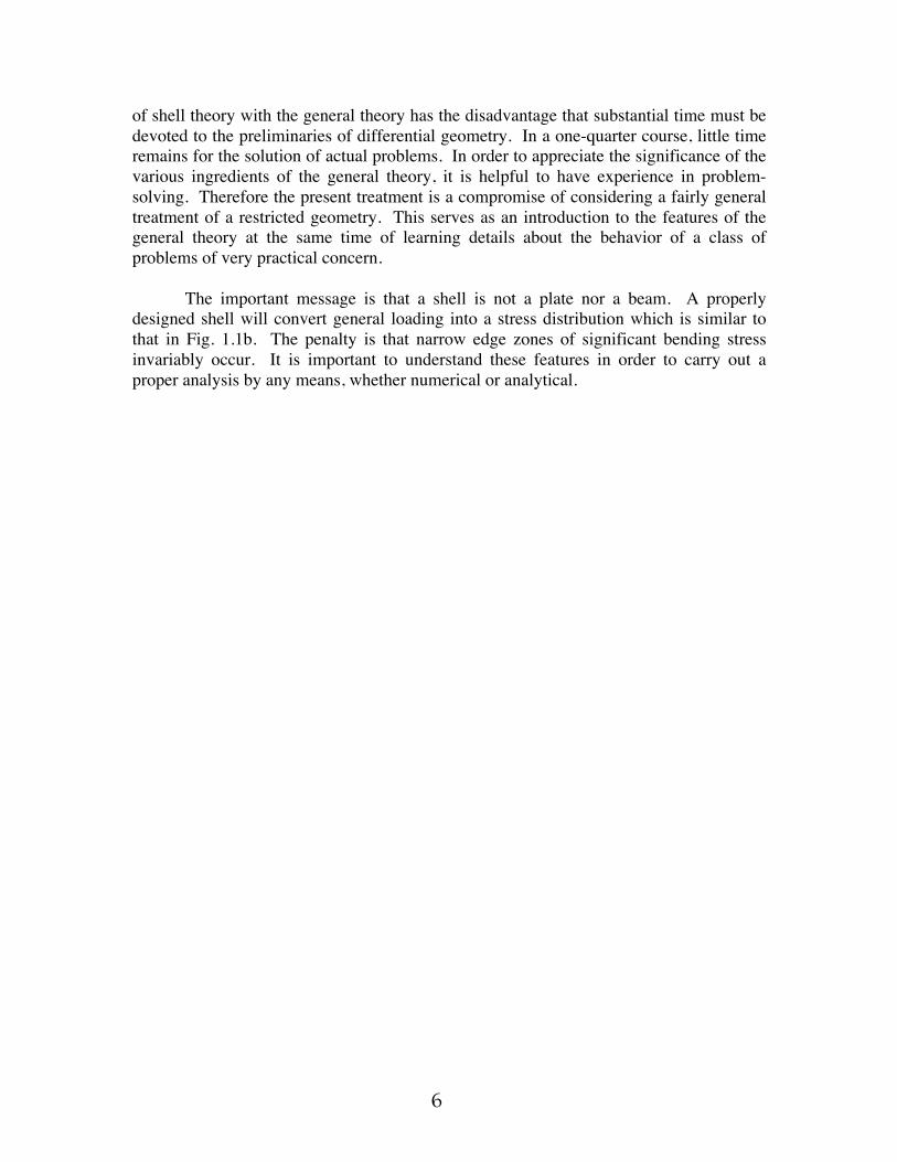
Figure 2.6 – Side view of element showing the stress resultants and surface load components. Either the components in the directions tangential and normal to the surface, or the components in the directions radial and axial may be used.

In Fig. 2.5 the components of force per unit length of the parallel circle ( s = constant ) are in the directions tangent and normal to the reference surface. It is convenient to work also with the components in the radial (horizontal) direction H and axial (vertical) direction V, as shown in Fig. 2.6: V = Ns sinϕ – Q cosϕ (2.4.1) H = Ns cosϕ + Q sinϕ (2.4.2) Components of surface loading in units of pressure, i.e., force per unit area, are used in both sets of directions: pV = ps sinϕ – pζ cosϕ (2.4.3) pH = ps cosϕ + pζ sinϕ (2.4.4)

18

The advantage of using the axial component of force is that the equation for axial equilibrium is easily obtained. The total axial force on the edge is 2πrV, so the equilibrium of the element of finite size is

Δ(2πrV) + pV 2π r Δs + O Δs2= 0 (2.4.5)

Taking the limit as the size of the element approaches zero gives the differential equation:

d r V d s

= – r pV (2.4.6) For this development of the equations, consideration of the changes from one side to the other of the element will be used. Elegance is lacking in this approach, but a physical understanding is gained. There is a limit to this approach in problems of more complexity, since the element consideration becomes too elaborate and susceptible to error. For example, in the theory of general shell surfaces, a vector-tensor approach using the divergence theorem is preferred. The equation (2.4.6) can be integrated:

r V = – r p V d s

s 0

s+ C

(2.4.7) in which the integration constant C must be the value of the left-hand side at the reference point of the meridian s0 : C = r V 0 (2.4.8) The consideration of the axial equilibrium is perhaps deceptively simple. Serious mistakes can be made if it is not kept clearly in mind that the axial forces must be balanced just as for the axial equilibrium of a rod. In the common situation when the surface loading and the axial force on one end of the shell are prescribed, (2.4.7) gives directly the axial resultant V. The remaining quantities are not so readily obtained.

19

Δ θ

H Δ θ r

H Δ θ r H Δ θ r + Δ ( )

Δ θ r pH Δs

N θ Δs

N θ Δs

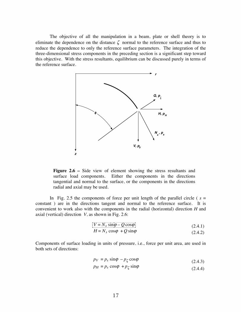
Figure 2.7a – View of the element showing the stress resultants which contribute to the equation for radial equilibrium.

Nθ Δ s cos Δθ 2

Nθ Δ s cos Δθ 2

Nθ Δ s sin Δθ 2

Nθ Δ s sin Δθ 2

Nθ Δ s

Nθ Δ s

Δθ

Nθ Δ s Δθ

Figure 2.7b – Top view of the element showing the contribution of the circumferential stress resultant to the equation for radial equilibrium.

For radial equilibrium, the result for the element shown in Fig. 2.7a is

Δ HrΔθ + pHrΔθΔs – N θ ΔθΔs + O Δs2Δθ = 0 (2.4.9)

which gives the differential equation:

20

– d r H

d s + N θ = r p H (2.4.10) In (2.4.9) the first two terms are similar to those for a beam; the crucial difference is in the Nθ term which arises from the curvature in the circumferential direction. The manner in which this circumferential resultant enters into the radial equilibrium equation is indicated in Fig. 2.7b.

Q r Δ θ

M s r Δ θ

Mθ Δ s cosφ

Mθ Δ s sinφ

Mθ Δ s sinφ

Mθ Δ s cosφ

Δ θ

Ms r Δθ + Δ Ms r Δθ

Figure 2.8 – View of the element showing the resultants which contribute to the equation for moment equilibrium.

For moment equilibrium, the significant resultants on the element are shown in Fig. 2.8, which give the equation:

Δ M s r Δ θ – Q r Δ θ Δ s – M θ cosϕ Δ θ Δ s ≈ 0 (2.4.11) which in the limit gives the differential equation:

–d r M sd s + M θ cos ϕ + r Q = 0

(2.4.12)

The moment M θ can be represented as a vector which is in the meridional direction.

This has a component in the axial direction which has the same magnitude on the two θ–faces of the element, which therefore cancel. The radial components on the two faces

21

change direction by the angle Δθ , and therefore contribute to (2.4.11-12) in the same

way that N θ contributes to (2.4.9-10).

A combination of the equations for axial and radial equilibrium provides the equation for normal equilibrium:

N sr1+N θr2– d r Q

r d s = p ζ (2.4.13)

This form shows clearly how the tangential resultants contribute to to support of the normal pressure because of the curvature. The equation for tangential equilibrium can also be obtained from a combination of the previous equations :

d r Nsd s

– cosϕ Nθ + Q rr1

= – r ps (2.4.14) These equations (2.4.12-13) can, of course, be obtained directly from a consideration of the element. The surface loads used (2.4.3-4) are in terms of the force per unit area of the reference surface. For thicker shells, it does make a difference whether the load is actually applied on the inner or outer surfaces. The correction for the pressure, which is loading in the normal direction, is

p ζ = p ζ ID 1 – t2 r1

1 – t2 r2

+ p ζOD 1 + t2 r1

1 + t2 r2 (2.4.15)

in which p ζID and p

ζOD are the forces in the normal direction per unit area of the inner

and outer surfaces, respectively. The signs of the radii of curvature will depend on the direction chosen for positive arc length. §2.5 Displacement according to Kirchhoff-Love Hypothesis The displacement components for a point on the reference are w and u in the normal and tangential directions, respectively. Alternately, the components h and v in the radial and axial directions can be used: h = w sinϕ + u cos ϕ (2.5.1) v = – w cosϕ + u sin ϕ (2.5.2) The rotation of the reference surface is

22

β = – d w

d s + u

r1 (2.5.3)

in which the first term is the same as for a beam or plate, while the u –dependence is due to the curvature. Alternately the rotation can be written in terms of the radial and axial displacements:

β = – d h

d s sin ϕ + d v

d s cos ϕ

(2.5.4) In order to obtain a reduction of the three-dimensional problem, it is necessary to relate the displacement at every point of the shell through the thickness to the displacement on the reference surface. The most simple and effective means for this is the kinematic assumption introduced by Euler and Bernoulli for beams, Kirchhoff for plates and Love for shells. In shell theory, this is usually referred to as the Kirchhoff-Love hypothesis. The assumptions are: (i) Points initially on the normal to the undeformed reference surface remain on a straight line during deformation, i.e., "normals remain straight". (ii) Points on the normal remain equidistant during deformation, i.e., "normals remain unstretched". (iii) The normal to the undeformed reference remains normal to the reference surface during deformation, i.e., "normals remain normal". If assumption (iii) is not made then the transverse shear deformation of the shell wall is permitted. This is significant when loading is localized or when the shell is composed of a composite with tangential fibers whose elastic modulus is large in comparison with that of the matrix. Removing assumption (ii) permits significant stretching and stress of the normal. This is also important for composites and for local contact problems. If assumption (i) is completely removed, the result is full three- (or for the present axisymmetric problem, two-) dimensional theory. A shell theory is retained by a partial relaxation of (i) by means of assumed polynomial expansions for the displacement through the wall thickness. The theory resulting from the elimination of (iii) and (ii) will be discussed in later sections. The relaxation of (i) has been discussed by many authors, but the most thorough treatment may be the recent work of Doxee (1987). For the present, the additional assumption is made that the displacement is small in comparison with the shell thickness and that all strain an rotation quantities are small in comparison with unity. Figure 2.9 shows the components of displacement.

23

r1

r

z

ζ

ϕ

w

uu + ζχ

χ

h

v

Figure 2.9 – Displacement for linear Kirchhoff-Love theory. The displacement of the point any distance off the reference surface is related to the reference surface displacement and rotation.

For the kinematic assumption (iii) that the normal remains normal to the reference surface, the rotation of the reference surface β and the rotation of the normal χ are the same:

β = χ (2.5.5)

The rotation is chosen to have the same sense of direction as the moment resultant M s on

the s–face of the element on the side of increasing s. Positive moment corresponds to tension in the shell outer surface. Thus, for any orientation of increasing arc length or of the z–axis, such as in Figs. 2.3a-c, the positive rotation is always clockwise. For the point a distance ζ from the reference surface, the initial radial and axial coordinates are

R 0 = r + ζ sinϕ (2.5.6)

Z0 = z – ζ cosϕ (2.5.7) After deformation, the normal displacement of the point is w from (ii), and from (iii) the tangential displacement is u + ζ χ. The radial and axial coordinates of the point then are: R = r + (ζ + w ) sinϕ + ( u + ζ χ ) cosϕ (2.5.8)

24

Z = z – ( ζ + w ) cosϕ + ( u + ζ χ ) sinϕ (2.5.9) §2.6 Strain The element Fig. 2.4 is used for the derivation of the "engineering" strain components in the shell. Easiest is the strain in the circumferential direction. The change in the circumference of a circumferential fiber divided by the initial length is

eθ =

2π R – 2π R 02π R 0 (2.6.1)

Substituting the values (2.5.5-8) yields the circumferential strain component

eθ =

w sinϕ + ( u + ζ χ ) cosϕr + ζ sinϕ (2.6.2)

The length before deformation of a fiber in the meridional direction, which is located the distance ζ from the reference surface, is

r1 + ζ Δϕ (2.6.3) while the length after deformation is

r1 + ζ + w Δϕ + Δ u + ζ χ (2.6.4) so that the change in length divided by the initial length is, in the limit, the meridional strain component

es =

w + d ud ϕ

+ ζ d χd ϕ

r1 + ζ (2.6.5)

The strain components (2.6.2) and (2.6.5) depend on both the reference surface displacements and the distance from the reference surface ζ. Taking ζ = 0 in these expressions gives the reference surface strain components:

εs = wr1

+ d ud s

(2.6.6)

εθ =

w sinϕ + u cosϕr (2.6.7)

25

which, in terms of the radial and axial displacement components, are

εs = d vd s

sinϕ + d hd s

cosϕ (2.6.8)

ε θ = hr (2.6.9)

The remaining quantities in (3.6.2) and (3.6.5) are the curvature change measures:

κ s = d χd s

(2.6.10)

κ θ =

χ cosϕr (2.6.11)

In terms of the strain measures, the strain components (2.6.2) and (2.6.5) are

e s =ε s + ζ κ s

1 + ζr1 (2.6.12)

eθ =εθ + ζ κθ

1 + ζr2 (2.6.13)

The curvature terms in the denominator cause some difficulty. However, for the simplest first- approximation theory for a thin shell, the denominators are replaced by unity, and these expressions have exactly the same form as for a flat plate or beam. Keeping the curvature terms does increase the accuracy significantly for thicker shells. For the situation in which the kinematic assumption (iii) is not made, then the transverse shear deformation must be included. The rotation of the reference surface β is not equal to the rotation of the normal χ . Thus (2.5.5) does not hold, and the difference between the two rotations is the measure of the transverse shear deformation γ :

γ = χ – β (2.6.14) All of the equations (2.5.6-9) and (2.6.1-13) are valid.

26

§2.7 Compatibility of Strain There are four strain measures:

εs , εθ , κ s , κθ (2.7.1)

which are functions of the two reference surface displacement components u and w. In the inverse problem of prescribing the four strain measures and then computing the two displacement components, the difficulty of having four equations and only two unknowns is encountered. For a solution, there must be two constraint conditions on the four equations. These are the compatibility of strain conditions. The elegant derivation is with the divergence theorem. For the present, the two conditions will be merely stated:

dd s

r κθcosϕ = κs

(2.7.2)

dd s

r εθ = εϕ cosϕ − β sinϕ (2.7.3) It is easy to substitute the expressions (2.6.6-7) and (2.6.10-11), with (2.5.3), into (2.7.2-3) and verify that the equations are identically satisfied. The relation (2.7.2) is rather trivial; however, (2.7.3) will be used in the subsequent development of the equations. In the computation of displacement from strain, the radial component could hardly be easier than from (2.6.9):

h = r ε θ (2.7.4) A relation for the vertical component is

d vd s

= β cos ϕ + εs sin ϕ (2.7.5) which can be verified by substitution of the expressions (2.5.4) and (2.6.8). For the tangential displacement, a useful identity is

d d s

usinϕ =

εs – εθ r2r1

sinϕ (2.7.6)

which can be verified by substitution of the expressions (2.6.6-7). Writing u in terms of the radial and axial components (2.5.1-2) gives

27

usinϕ = v + h cotϕ

(2.7.7) Thus either (2.7.5) or (2.7.6) can be integrated to obtain the axial displacement. The constant of integration is, of course, the axial rigid body displacement. §2.8 Constitutive Equations Before the shell, it may be of value to consider the behavior of a beam, as indicated by elementary bending theory. For a cantilever beam of length L and thickness t, with end load Q per unit width, the maximum stress at the support is

σmax =M cI =

Q L t2

t312

= Qt6 Lt

(2.8.1) Thus the average transverse shear stress Q /t produces a tangential bending stress which is of the order of magnitude of L /t larger. The transverse shear resultant is certainly important, as in this problem, but the transverse shear stress is small in comparison with the tangential stress when the beam is slender. This is the general situation for beams, plates and shells, and is the reason that the kinematic hypotheses in section §2.5 work so well. When the same beam is loaded by a transverse pressure p, the result for the maximum stress is

σ max =M t /2

I =p L 2

2t2

t312

= p 3 L 2

t2

(2.8.2) The surface pressure p is the normal stress component, which is very important to the problem, since without it, there would be no problem. However, the tangential stress produced is much larger for a thin beam. These are rather simple examples, but they do demonstrate the general principle that the transverse shear stress and normal stress are relatively small for a structure whose length is much greater than the thickness. §2.8.1 Isotropic Shell The linear, three-dimensional, stress-strain relations for an isotropic elastic body (Hooke's law) are

E e s = σ s – ν σ θ – ν σ ζ (2.8.3)

E e θ = σ θ – ν σ ζ – ν σ s (2.8.4)

28

E e ζ = σ ζ – ν σ s – ν σ θ (2.8.5) in which ( s, θ, ζ ) are any orthogonal coordinates, E is Young's modulus and ν is Poisson's ratio. In addition there are relations between the shear stress and strain. For the thin plate and shell

σζ << σs , σθ (2.8.6) so that (2.8.3-5) are approximately

E eζ = – ν σs – ν σθ (2.8.7)

σs =E

1 – ν2es + ν eθ

(2.8.8)

σθ =E

1 – ν2eθ + ν es

(2.8.9) The result for the strain of the normal (2.8.7) violates the kinematic hypothesis (ii) in section §2.5. However, the adjustment of the normal distance indicated by (2.8.7) has a small effect on the tangential strains (2.6.10-11). The strains in the form (2.6.12-13) are substituted into (2.8.8-9), which are substituted into (2.3.2-4) and (2.3.6-7), yielding the results:

Νs = E1 – ν2

ε s + ζ κs 1 +

ζr2

1 + ζr1

+ ν ε θ + ζ κθ

– t /2

t /2

d ζ

(2.8.10)

Μs = E1 – ν2

ε s + ζ κs 1 +

ζr2

1 + ζr1

+ ν ε θ + ζ κθ

– t /2

t /2

ζ d ζ

(2.8.11) The expressions for the θ -components are similar. Love's first approximation theory is obtained by assuming that the shell is very thin:

29

t << r1 , r2 (2.8.12) Then all the curvature terms in (2.8.10-11) can be neglected. The result looks exactly like the relations for a flat plate:

Νs = E1 – ν2

ε s + ζ κs + ν ε θ + ζ κθ– t /2

t /2

d ζ

(2.8.13)

Μs = E1 – ν2

ε s + ζ κs + ν ε θ + ζ κθ– t /2

t /2

ζ d ζ

(2.8.14) For the case of transverse homogeneity, in which E and ν are independent of ζ , (2.8.13-14) and the similar expressions for the circumferential direction reduce to the familiar relations:

Ν s =E t

1 - ν2

εs + ν εθ (2.8.15)

Νθ =E t

1 - ν2

εθ + ν εs (2.8.16)

Μ s =E t 3

12 1 - ν2

κ s + ν κθ

(2.8.17)

Μθ =E t 3

12 1 - ν2

κθ + ν κ s (2.8.18)

Because the factor must be written many times, we introduce the reduced thickness c:

c2 = t2

12 1 − ν2

(2.8.19) Even though (2.8.15-18) appear to be the same as for a flat plate, the strain measures do retain the curvature effects of the shell. For the inclusion of transverse shear deformation (2.6.14) the relation between the shear strain measure and the transverse shear must be used:

30

Q = E t

µχ – β

(2.8.20) in which E / µ is the effective transverse shear modulus. For an isotropic shell wall, µ is around 3. For a composite or sandwich construction, µ may be large. §2.8.2 Composite Shell A composite shell wall may consist of many layers, each of which has different orthotropic elastic properties, as discussed by Christensen (1979). When the coordinate axes are also elastic symmetry axes, the analysis for the isotropic material can be readily extended to the composite. This includes sandwich construction or a construction with rings and stiffeners which are sufficiently closely spaced to be "smeared", i.e., treated as a wall with uniform thickness with equivalent orthotropic properties. Instead of (2.8.8-9) the layer stress-strain relations are written as

σsσθ

= Q11 Q12Q21 Q22

eseθ

(2.8.21)

in which the coefficients are related to the directional Young's moduli and Poisson's ratios of the layer by

Q11 =

E111 - ν12ν21 (2.8.22)

Q12 =

E11 ν211 – ν12ν21 (2.8.23)

Q21 =

E22 ν121 – ν12ν21 (2.8.24)

Q22 =

E221 – ν12ν21 (2.8.25)

The integration for the resultants, instead of (2.8.15-18), yields

N sN θM sM θ

= 0B 1B1B 2B

ε sε θκ s

κ θ (2.8.26)

31

in which the elements of the matrix are 2x2 matrices with the coefficients

j B 11 = Q 11

1 + ζr2

1 + ζr1

ζjd ζ

– t / 2

t / 2

(2.8.27)

j B 12 = Q 12 ζ

jd ζ

– t / 2

t / 2

= j B 21

(2.8.28)

j B 22 = Q 22

1 + ζr1

1 + ζr2

ζjd ζ

– t / 2

t / 2

(2.8.29) The difficulties with composites are not with the calculation of these equivalent moduli. §2.9 Computation of Stress from Stress Resultants The three-dimensional stress in the shell wall is integrated to obtain the stress resultants. After a problem is solved in terms of the resultants, the question arises of how the stress is best computed. Obviously it is impossible to reconstruct the details of a stress distribution through the thickness from only the resultant force and moment. The first approximation (2.8.12) was the justification for dropping the curvature terms in (2.8.10-11). If the same terms are deleted in (2.6.10-11), a linear distribution of strain and hence stress through the thickness is obtained, just as in elementary beam theory (2.8.1-2). The result for the stress distribution is

σss ≈ σsD + σsB

2 ζt (2.9.1)

where the average "direct" or "membrane" stress is

σsD =

Ν st (2.9.2)

32

and the "bending" stress is

σsB =

6Μ s

t2 (2.9.3) The stress on the outer (OD) and inner (ID) surfaces is therefore

σsOD = σsD + σsB (2.9.4)

σsID = σsD − σsB (2.9.5) with similar expressions for the θ-direction. For better accuracy, however, the curvature terms in (2.6.12-13) should be retained. Some examples for thick shells will be shown later, in which substantial accuracy can be gained by a first approximation calculation of the stress resultants and strain measures, followed by the use of the exact expressions (2.6.12-13) for the strain and (2.8.8-9) for the stress. This certainly true for the composite shell, for which the stress distribution calculated from (2.8.21) may deviate substantially from linear. §2.10 Boundary Conditions At each edge of a shell, either the stress resultants, the displacements or a linear combination of stress resultants and displacements may be prescribed. §2.10.1 Edge Tractions The resultants which can be prescribed are shown in Fig. 2.10a. Important is that

the radial resultant H and the moment M s are each self-equilibrating for the present

axisymmetric problem. The load per unit length on one side of the shell edge balances the load on the opposite side of the circumference. By the principle of St. Venant, a self-equilibrating system of tractions on a region of the boundary of an elastic body are expected to cause a state of stress in the body which diminishes with the distance from

the boundary region. Indeed, M s and H can be prescribed independently on the two

edges and do cause a stress in the shell which is local to the the edge region when the shell is sufficiently long. This is a total of four independent scalar conditions. In contrast, the axial resultant V, when integrated around the circumference at one edge, has a resultant axial force which must be balanced by the distribution of V at the other edge. This is the fact which was used for the equation of axial equilibrium (2.4.7). For the most common problems, the axial load on one edge and the surface loads are prescribed, so that V is statically determinant from (2.4.7).

33

zV

pH

pV

M s

H M s

V

H

s

r

M s

H

V V

H

(a)

zv

h

v

h

s

rh

v v

h

(b)χ χ

χχ

Figure 2.10 - Quantities which can be prescribed on the shell edges: (a) Stress resultants, (b) Displacement and rotation

§2.10.2 Edge Displacements The edge displacements are shown in Fig. 2.10b. The directions of the displacement components and the rotation on all edges are shown as a reminder that these quantities have the same direction at both edges of the meridian. The stress resultants shown in Fig. 2.10a have opposite directions at the two edges. The directions of the displacements are chosen to have the same direction as the resultants on the positive s -face. It is possible to prescribe the radial displacement component and the rotation independently at the two edges, giving four independent scalar conditions. In addition it is possible to prescribe the axial displacement independently at the two edges. The average value is, however, merely the rigid body translation. The difference in axial displacement causes a stretching of the shell, which is a significant stress state but one related to the constant in (2.4.7) which provides a constant axial force.

34

§2.10.3 Edge Stiffness Counting both edges in Fig. 2.10, there are a total of six edge resultants and six edge displacements ( including rotation ). The condition of axial equilibrium makes the axial resultant on one edge dependent, and the average axial displacement is a rigid body translation. Thus there are a maximum of five scalar conditions. If the edges of the shell are attached to springs ( or to other shells ) then the general boundary condition can be written in the matrix form:

M sHV 1

M sH 2

= B

χh 1

v 2 - v 1

χh 2

+ Bp

(2.10.1) in which the subscripts 1 and 2 denote values at the negative and positive s -faces,

respectively. The matrix B is the matrix of stiffnesses from the attachments and B p is a

vector of prescribed loads. §2.11 Differential Equations By following the formulation of E. Reissner (1960), all the preceding equations are reduced to a system of the fourth order, consisting of a pair of coupled differential equations each of the second order. Such a system of equations was first obtained by H. Reissner (1912) and Meissner (1915). The advantage of the formulation of E. Reissner is in the explicit use of the axial and radial resultants. Then the technique of Novozhilov (1959) for the general shell surface is utilized to obtain a single equation of the second order, but with a complex dependent variable. In this section, zero transverse shear deformation is assumed. §2.11.1 Reissner System The starting point is consideration of the equation of compatibility (2.7.3) and the equation of equilibrium (2.4.12), which are rewritten in the form:

d r εθd s

– εs cosϕ + χ sinϕ = 0 (2.11.1)

d r Ms

d s – Μθ cosϕ – r H sinϕ = – r V cosϕ (2.11.2)

35

The constitutive equations and the remaining equations are used to reduce (2.11.1-2) to the following form first given by E. Reissner (1949):

E t c2 d

d s r

d χd s

+ –ν sinϕr1 –

cos2ϕr χ – r H sinϕ = – r V cosϕ (2.11.3)

1

E t d

d s r d r H

d s + ν

sinϕr1

– cos2ϕ

r r Η + χ sinϕ =

1E t

– dd s r2 pH – ν r V sinϕ + cosϕ V sinϕ – ν r pH (2.11.4)

Since the axial resultant V is determined from (2.4.7), it appears in the equation as a known load term on the right-hand side. The system is then of the fourth order. §2.11.2 Novozhilov Complex Equation Because of the similarity of the two equations (2.11.4-5), they can be combined by the following device. Multiply the first equation (2.11.3) by -ik -1 , where i is the imaginary unity and k is a constant, then add the result to the (2.11.4). If the elastic moduli E and ν and the thickness t are all constant, then k is chosen as k = E t c (2.11.5) and the following complex quantities is introduced:

H = H - i k χ r-1 (2.11.6) The complex conjugate is

H = H + i k χ r-1 (2.11.7) The combined equation is then:

- i c d d s

r d r Hd s

- cos2ϕ Η + ν sinϕr1

r H + rH sinϕ = rV cosϕ (2.11.8) in which the complex axial resultant is

V = V + i c

r 1cosϕ d

d s r2 pH – ν r V sinϕ – V sinϕ + ν r pH

(2.11.9)

36

The problem is that the complex conjugate remains in the equation. However, consider the two terms on the left-hand side of (2.11.8):

- i c νr1

H + H r sinϕ (2.11.10)

The complex conjugate is multiplied by a term which is zero for zero Poisson's ratio and for a conical or cylindrical shell, and is generally of the magnitude of the thickness divided by the radius of curvature of the surface. Since such terms have previously been neglected (2.8.12), it seems consistent to drop such a term here, and the final equation is obtained:

- i c d d s

r d r Hd s

- cos2ϕ Η + rH sinϕ = rV cosϕ (2.11.11) With the solution of this equation, the stress resultants can be computed from the formulas:

N θ = Re d r H

d s + r pH (2.11.12)

N s = H cosϕ + V sinϕ (2.11.13)

Q = H sinϕ – V cosϕ (2.11.14)

Ms = – c I m d rH

d s + ν H cosϕ (2.11.15)

Mθ = – c I m ν d rH

d s + H cosϕ (2.11.16)

It is typical in shell theory that many terms are encountered in the equations which clutter up the proceedings but which are negligible within the inherent error of the theory. However, one must be wary of dropping terms which seem to be small at one point in the system of equations, since such terms may be of primary importance at a later point in the manipulation. The order of magnitude argument for deleting the "junk" terms was used by Novozhilov (1959), but we have followed Baker and Kline (1962) who introduced the conjugate, which makes the argument clearer. Still, the argument is not totally convincing since the real and imaginary parts of (2.11.10) are not considered independently. So far as is known, there is not an example in which serious errors are encountered with the use of (2.11.11).

37

The equation (2.11.11) is of the second order and so will have two linearly independent solutions. These solutions are complex valued, and the real and imaginary parts provide the total of the four linearly independent solutions needed. The advantage of the equation (2.11.11) is that an equation of the second order is easier to solve, or discuss, than a system of fourth order. The difficulties caused by various geometries are rather transparent and can be handled by techniques which have been extensively treated in the mathematical literature. The disadvantage is that the equation is restricted to the the linear behavior of the homogeneous, isotropic shell of constant thickness. Relaxation of any of these restrictions leads to an equation in which the complex conjugate cannot be argued away. In this case, the equation must be separated into real and imaginary parts for a solution, which is equivalent to working with the original real system. Thus if the conjugate remains in the complex equation, no real gain is accomplished. §2.11.3 Matrix Equation A third approach to an appropriate casting of the general equations into a form suitable for solution is simply to leave the equations as a system of first-order equations. This has a definite advantage in that additional effects can be readily incorporated, without the necessity of repeating an elaborate equation manipulation. More important is that there are definite numeric and analytic advantages in considering a matrix system. Some manipulation is still required in order to obtain a system in which appear only the displacement and force quantities which may be prescribed on the boundaries. The equations are selected in which the derivatives of the desired quantities appear. The equilibrium equations (2.4.12) and (2.4.10), and the kinematic relations (2.6.10), and (2.7.3) are collected:

dd s

r Ms

r H

χ

h

=

Mθ cosϕ + r H sinϕ – r V cosϕ

N θ – r pHκ s

εs cosϕ – χ sinϕ (2.11.17)

The remaining equations are used to eliminate the dependent quantities, the quantities which cannot be prescribed on the edges, from the right-hand side. For this, the constitutive relations (2.8.15-18) must be partially inverted:

38

εs = – ν hr + 1 - ν2

E t H cosϕ + V sinϕ

Nθ = E t hr + ν H cosϕ + V sinϕ

κs = MsE t c2

– ν χ cosϕ

r

Mθ = ν Ms + E t3

12 χ cosϕr (2.11.18-21)

These relations used in (2.11.17) yield the matrix equation:

− d Yd s + A•Y = P (2.11.22)

in which the vector of the stress and displacement quantities is

Y =

r M s

r H

χ

h (2.11.23) the coefficient matrix is

A =

ν cosϕr sinϕ E t3

12 cos2ϕ

r 0

0 ν cosϕr 0 E t

r

1r E t c2

0 – ν cosϕr 0

0 1 – ν2 cos2ϕr E t

– sinϕ – ν cosϕr

(2.11.24) and the load vector is

39

P =

r V cosϕ

r pH – ν V sinϕ

0

– 1 − ν2

E t V sinϕ cosϕ

(2.11.25) Some advantages of working directly with the matrix equation are: (1) The quantities of interest are treated simultaneously. In the reduction to a single scalar equation, such as (2.11.11), certain variables are selected. The remaining quantities which are needed for the boundary conditions must be evaluated by working back through the system. Even for the present, fairly simple problem, this involves the derivative of the solution in (2.11.12-16). (2) The derivatives of the material properties are avoided. Discontinuity in the geometry and material means that A is discontinuous. Although (2.11.11) is restricted to constant material properties, if one would work out a single scalar equation for the general problem, higher derivatives of the material properties would appear. (3) The matrix form is ideal for the analytic procedure of asymptotic expansion. (4) The matrix form has advantages for direct numerical computations. §2.12 Variational Formulations The procedure which has been followed for the derivation of the equations emphasizes the physical meaning of the various terms and equations. An alternate approach is to consider the potential energy. Equations can be directly obtained without so much chance of error. Furthermore the potential, or the more general Galerkin formulation, provides the stating point for finite element calculations. There is considerable information on this in a variety of sources on the literature. The variational problem has the form:

δ L d s

s 1

s 2+ R = 0

(2.12.1) in which δ indicates the first variation, L is the energy density and R is the potential of the

40

edge loads. For this consideration it is actually easier if the transverse shear deformation is included. §2.12.1 Transverse Shear Deformation In the strain energy formulation, the density is

LSE =Ε t c2

2κ s2+ 2 ν κ s κθ + κθ

2+

Ε t

2 1 – ν2

εs2+ 2 ν εs εθ + εθ

2

+ E t2 µ

χ – β2– p s u - p ζ w 2π r

(2.12.2) in which the terms of strain energy in bending, stretching, transverse shear deformation and the potential of the surface loads appear. The factor of 2πr comes from the integration around the circumference of the shell. In the complementary energy formulation, the constitutive relations are used to write (2.12.2) in terms of the stress resultants, with the result:

LCE = 12

2 Ε t3 Μs

2 – 2 ν Μs Μθ + Μθ2 + 1

2 Ε t Νs

2 – 2 ν Νs Νθ + Νθ2

+ µ

2 E tQ 2 – p s u - p ζ w 2π r

(2.12.3) A mixed formulation, developed by Hellinger, Reissner, Hu and Washitzu, has both the resultants and the strain measures:

LR = Μ s κ s + Μθ κθ + Ν s εs + Νθ εθ + Q χ – β

– 12

2 Ε t3 Μs

2 – 2 ν Μs Μθ + Μθ2 – 1

2 Ε t Νs

2 – 2 ν Νs Νθ + Νθ2

– µ

2 E tQ 2 – p s u - p ζ w 2π r

(2.12.4) This formulation for various problems in mechanics has been shown by several investigators to have substantial advantages, particularly because the stress and displacement quantities are treated equally and simultaneously. It is desirable for our present shell of revolution problem, however, to write the energy density only in terms of the elements of the vector (2.11.23), using the relations

41

(2.11.18-21) which were used to obtain the matrix equation. First, the circumferential resultants are eliminated, giving a modified Reissner form:

LRM = Μ s κ s + ν κθ + Ν s εs + ν εθ + Q χ – β

+ 12E t3

12 κθ

2+ E t εθ

2– 12

Ms2

E t c2+N s2 1 – ν

2

E t+ µ Q2

E t

– p s u - p ζ w 2π r (2.12.5) Then the tangential and normal stress resultants are replaced by the axial and radial. The result can be condensed to the following vector form (dropping the 2π factor):

L RM = F•d Dd s + D

t•E•F – 12 Ft•C•F + 12 D

t•K•D + F t•G – D t•B (2.12.6)

in which the superscript t indicates the transpose, the vector (2.11.23) is partitioned into a "force" vector and a "displacement" vector:

F = r M s

r HD =

χh (2.12.7)

and the matrices are:

E =νcosϕr sinϕ

0 νcosϕr (2.12.8)

C =

1r E t c 2

0

0 1 - ν2cos2ϕ + µ sin2ϕr E t

(2.12.9)

K =

E t 3 cos2ϕ12 r 0

0 E tr (2.12.10)

42

The matrices C and K have terms of "compliance" and "stiffness", respectively. The "load" vectors are

B = r V cosϕ r pH – ν V sinϕ G =

0

– 1 – ν2 – µ

E t V sinϕ cosϕ

(2.12.11) The Euler-Lagrange equations of the variational problem are obtained by considering the variation of the force vector:

∂ L MR∂ F = d Dd s + E

t•D – C•F + G = 0 (2.12.12)

and then considering the variation of the displacement vector:

– dd s

∂ L MR

∂ d Dd s

+∂ L MR∂ D = – d Fd s + E•F + K•D – B = 0

(2.12.13) The two can be written together as

– dd s

FD +

E KC – E t

FD = B

G (2.12.14) which is exactly the system previously derived (2.11.22) with

Y = F

D A =E KC – E t

P = BG (2.12.15)

The only difference is that the transverse shear deformation term µ is included in (2.12.9) and (2.12.11). The variational approach provides the structure of the coefficient matrix A, which consists of the two symmetric submatrices C and K and the nonsymmetric matrix E. §2.12.2 Moderate Rotation Until this point, only the linear theory has been considered. Important in many problems are nonlinearities, which may be due to material behavior at strains higher than the yield point, or may be due to geometric effects of large displacement and rotation. The geometric nonlinearities are particularly significant for the stiffening of thin shells in

43

regions of high tension, and for the collapse or buckling in regions of sufficiently high compression. It is remarkable that much of the geometric nonlinear effect can be included by means of the moderate rotation theory. It is assumed that the strains are small, which means, that the radial displacement h (2.6.9), and the derivative of the tangential displacement u (2.6.6) must be small. However, the rotation β (2.5.3) depends on the derivative of the normal displacement w, which may not be small. Therefore, terms involving the square of the rotation are retained. For plates, this leads to the equations of von Kármán. For shells, a variety of equations have been utilized which differ in detail but have the same essential features. The variational formulation provides an extremely simple derivation of the theory for the present axisymmetric case. The basic ingredient is the same as in beam theory and consists of adding the rotation effect to the meridional strain. Thus the following replacement is made in (2.12.2), (2.12.4) or (2.12.5):

εs +

12 β

2⇒ εs (2.12.15)

The rotation of the reference surface is related to the rotation of the normal by the constitutive relation (2.8.20), with which the energy density (2.12.5) becomes

LRM = Μ s κ s + ν κθ + Ν s εs + ν εθ + Q χ η – β + 12 N s χ

2

+ 12E t3

12 κθ

2+ E t εθ

2– 12

Ms2

E t c2+N s2 1 – ν

2

E t+ µ Q2η

E t

– p s u - p ζ w 2π r (2.12.16) in which η is the factor:

η = 1 –

µ N sE t (2.12.17)

The second term in this factor is the ratio of direct stress to the effective transverse shear modulus. If this is small, then

η ≈ 1 (2.12.18) and only one additional term appears in (2.12.16). This creates two additional terms in the coefficient matrix of the differential equation (2.11.22) or (2.12.14). The corrected coefficients of A are

44

a13 = E t3 cos2ϕ12 r

+ r Ns (2.12.19)

a43 = – sinϕ – 12 χ cosϕ

(2.12.20) The meridional stress resultant in the coefficient (2.12.19) is the important "prestress" term which crucial for the analysis of bifurcation buckling. The rotation term in (2.12.20) tends to be important in local regions. Note that (2.12.19) does not disturb the form of the system (2.12.15) since this is a diagonal term of the K matrix. The extra nonlinear term in (2.12.20) does not fit the form of (2.12.15) since a similar term does not

appear in the coefficient a 12 , i.e., the coefficient e

12 of E. §2.12.3 Vibration of Composites The form (2.12.14) is obtained in mechanics for systems of mechanics which are self-adjoint, which means that they can be obtained from a variational principle. Very general discussion of these systems is given by Abraham and Marsden (1978). In this section, it is shown that the equations for the vibration of a general composite can be reduced to this form. For this purpose, the constitutive relations (2.8.26) are written as:

M sQN s

M θN θ

=Γ11Γ12

Γ21Γ22

κ s

χ –β

ε s

κ θ

ε θ (2.12.21)

in which the quantities which can prescribed on the edge are separated from those which cannot, and the transverse shear deformation is included. In dynamics, the axial component of force is not statically determinant, so these components will be included as unknowns. As done by Fettahlioglu and Steele (1974), this system can be partially inverted to the form:

45

κ s

χ –β

ε s

M θN θ

=Φ11Φ12

Φ21Φ22

M sQN s

κ θ

ε θ

(2.12.22) in which

Φ11 = Γ11–1

Φ21 =Γ21•Γ11–1= – Φ12

t

Φ22 = Γ22 – Γ21•Γ11–1•Γ12 (2.12.23)

The potential density (2.12.16) can be written as:

LRM = Μs Q Ns •κs

χ – β

εs

+ Φ2 1t • κθεθ

+ 12

κθ εθ •Φ22•κθεθ

– 12

Μs Q Ns •Φ11•

Μs

Q

Ns

+ 12 χ h v •Kspring•χhv

– χ h v •mpHpV

2π r

(2.12.24) in which a moment loading m per unit of reference surface area is included, as well as a matrix of springs attached to the surface:

K spring =

k m 0 0

0 k H +k s cos2ϕ + k ζ sin

2ϕ k s – k ζ sinϕ cosϕ

0 k s – k ζ sinϕ cosϕ k V +k s sin2ϕ + k ζ cos

2ϕ

(2.12.25)

46

For vibration and wave propagation, all variables can be considered to have the time dependence eiωt where ω is the frequency. Although this may have a profound effect on the solution and the appropriate solution procedure, small amplitude dynamics is easily include into the equations by subtracting the inertia terms from the spring stiffnesses:

k m – ρ ω2t3/12⇒ k m

k H – ρ ω2t ⇒ k H

k V – ρ ω2t ⇒ k V (2.12.26-28)

The rotary inertia (2.12.26) and the transverse shear deformation are the terms included in the Timoshenko beam theory, which provide the correct wave propagation properties absent from the elementary beam theory and, it should be added, better accuracy when the wavelength of deformation is small. The task is now to write (2.12.24) in terms of the resultants in the radial and vertical directions by defining the "force vector" as

F =r M sr Hr V

= G 1–1•

r M sr Qr N s (2.12.29)

where the transformation matrix is

G 1 =1 0 00 sinϕ – cosϕ0 cosϕ sinϕ (2.12.30)

with

G 1t = G 1

–1 (2.12.31)

The "displacement vector" is

D =χhv (2.12.32)

47

in terms of which the strain measures can be written:

κ s

χ – β

ε s

= G 1•d Dd s + G 2•D

(2.12.33)

κ θ

ε θ= 1r G 3•D

(2.12.34)

in which G 2 has only one nonzero element:

G 2 =

0 0 01 0 00 0 0 (2.12.35)

and

G 3 =

cosϕ 0 00 1 0 (2.12.36)

The result is exactly the form (2.12.6) with

E t = G 1

t • 1r Φ21

t•G3 + G 2 (2.12.37)

K = 1r G 3

t •Φ22•G3 + r K spring (2.12.38)

C = 1r G 1

t •Φ11•G1 (2.12.39) and the load term is

B =

r mr pHr pV

(2.12.40)

Thus for the most general constitutive relations which include full coupling between bending and stretching effects in the shell, the final equation (2.11.22) or (2.12.14) can be formed by direct matrix operations.

48

For the first approximation theory for the isotropic shell, the matrices reduce to:

Γ11 =

Ε t c 2 0 0

0Ε t

µ0

0 0Ε t

1 − ν2

(2.12.41)

Γ21 =

ν Ε t c 2 0 0

0 0 ν Ε t

1 − ν2

(2.12.42)

Γ12 = Γ21t

(2.12.43)

Γ22 =

Ε t c 2 0

0Ε t

1 − ν2

(2.12.44)

Φ21 = Γ21•Γ11

–1 = ν 0 00 0 ν

(2.12.45)

Φ22 = Γ22 – Γ21•Γ11

–1•Γ12 =

Ε t3/ 12 0

0 Ε t (2.12.46) which yield

49

E =

ν cosϕr sinϕ – cosϕ

0 ν cosϕr

ν sinϕr

0 0 0 (2.12.47)

K =

E t 3cos2φ12 r

0 0

0 E tr 0

0 0 0

+ r Kspring

(2.12.48)

C =

1E t c2

0 0

0 µ sin2ϕ + 1– ν2 cos2ϕr E t

1– ν2– µ cosϕsinϕr E t

0 1– ν2– µ cosϕsinϕr E t

µ cos2ϕ + 1– ν2 sin2ϕr E t

(2.12.49)

50