the effect of curvature on turbulence in stratified fluids · the effect of curvature on turbulence...

JOURNAL OF GEOPHYSICAL RESEARCH, VOL. 95, NO. Cll, PAGES 20,313-20,330, NOVEMBER 15, 1990

The Effect of Curvature on Turbulence in Stratified Fluids

L. H. KANTHA

Institute for Naval Oceanography, Stennis Space Center, Mississippi

A. ROSATI

Geophysical Fluid Dynamics Laboratory, Princeton, New Jersey

The influence of streamline curvature on small-scale turbulence and vertical mixing in stratified fluids is the subject of this study. The roles of curvature and stratification in enhancing and suppressing turbulent mixing are explored using second-moment closure for turbulence. Governing equations for second moments are expressed in generalized orthogonal curvilinear coordinates, from which, through a series of approximations, simplified expressions are derived for second moments in the limit of small streamline curvature. The governing equations are then used to obtain a quasi-equilibrium turbulence model suited for application to atmospheric and oceanic mixed layers. A typical model application is illustrated by simulation of stratified flows over two-dimensional, idealized mountains and valleys. The limit of local equilibrium is further invoked to derive semi-analytical results for the enhancement and suppression of vertical'turbulent mixing under the combined influence of stratification and curvature. It is shown that stabilizing curvature can drastically suppress turbulence even when the stratification is strongly destabilizing. Conversely, under strong stable stratification that would otherwise lead to total suppression of turbulence, destabilizing curvature can keep turbulence alive. Streamline curvature is also shown to significantly modify the Monin-Obukhov similarity laws for momentum and heat fluxes in the constant flux region of the atmospheric boundary layer. Finally, the need for observational data on curvature effects on mixing in stratified flows either in the laboratory or in flows over topography in the oceans and the atmosphere is highlighted.

1. INTRODUCTION

The effects of streamline curvature and gravitational stratification acting together on turbulence in a mixed layer is the subject of this paper. This problem is of considerable geophysical interest in mesoscale flows over topography. The flow of stably stratified atmosphere over mountains and valleys leads to the generation of strong internal gravity waves, which can break aloft and lead to a strong divergence of momentum flux. Consequently, mountains can exert a large drag on the atmosphere and can significantly influence the skill of medium-range weather forecasts. More accurate mountain drag parameterization in medium range weather prediction models could improve their forecast skill. The momentum flux due to gravity waves propagating upward from the troposphere is also an important factor in the dynamics of the middle atmosphere. In the oceans, too, it might be important to account for curvature effects in understanding and modeling of flows over seamounts, especially those straddling energetic streams (for example, the Emperor seamounts in the Kuroshio's path). Therefore a better understanding of flow over topography is of some importance for many practical reasons.

Traditionally, in considering flows over topographic changes, not much importance has been given to accurate parameterization of turbulence and its generation and dissipation in the atmosphere. Most often, rather arbitrary sta- bility dependent mixing coefficients have been used in simulations of such flows. The influence of the atmospheric boundary layer and, to some extent, the effect of rotation has also been traditionally ignored. This is understandable be-

Copyright 1990 by the American Geophysical Union.

Paper number 90JC00489. 0148-0227/90/90J C-00489 $05.00

cause of the focus on the low-drag regime, in which the waves do not break and therefore turbulent mixing regions do not form in the flow aloft. However, in the so-called high-drag regime, the intense turbulent regions created in the lee of mountains by breaking gravity waves call for a more careful look at the turbulence parameterization itself. In any event, the turbulence in the atmospheric boundary layer flowing over the topography itself needs to be taken into account in both low- and high-drag regimes. Therefore a careful examination of the behavior of turbulence in strati-

fied flows over topography is helpful to our understanding of such flows.

At a first glance, one might be tempted to ignore the effect of surface curvature on turbulence in stratified flows over

topography. It is natural to assume that the curvature effects are secondary, while stratification exerts a dominating influence on turbulence. Such an assumption needs to be put to a rigorous test, however. It is not at all clear a priori that curvature effects are always negligible. There might be some situations where these effects become large, if not dominant. In any case, the effects should be quantified in order to make it possible to delineate circumstances where the effects of curvature are negligible and those where they are not. The governing parameters and their plausible ranges need to be explored. The object of this study is to do precisely that. We will employ second-moment closure of turbulence to inves- tigate the properties of turbulence under the combined action of stratification and curvature. It is important to note that the additional terms that result in the equations do not present any closure problems. In fact, these terms do not have to be modeled. This certainly is a decisive advantage, since it removes the uncertainty of the precise manner of their modeling on the results. The interpretation of the

20,313

20,314 KANTHA AND ROSATI: EFFECT OF CURVATURE ON TURBULENCE

effects of curvature therefore becomes rather straightforward.

2. GOVERNING EQUATIONS

It is convenient and appropriate to start an investigation of the effects of flow curvature on turbulence by rewriting the governing equations in generalized orthogonal curvilinear coordinates. It is then possible to proceed in an orderly fashion from the case of arbitrary curvature to the geophys- ically important case of small curvature. The derivation of the general form of these equations is necessarily cumber- some and is best omitted here. We will therefore present these equations without any derivation, making note of the fact that the turbulence closure approximations have already been incorporated into these equations (see Mellor and Yarnada [1982] and Galperin et al. [1988] for a discussion of these approximations in particular and second-moment closure in general). We have also ignored any implicit curvature terms in the Rotta approximation for pressure-strain covariance terms (see Appendix A). It is straightforward though lengthy and time consuming for the reader to derive these equations by starting from momentum and heat balance equations in orthogonal curvilinear coordinates and using standard procedures for derivation of equations for second moments of turbulence quantities [see Hinze, 1975].

The equation for Reynolds stresses in tensohal form is

0 (U-•) q- UiU j q- UiU j --• q-- O• • hi O•k hj

• 10hk 1 ohk'• .... llitlk hi oei

{, Ohihh3) + u•uiuj hi4.h 3 o• • h•

ukujuk Oh• u•uiu• Ohk'• hih• oei h•h• •j

=

hi V• • •hiVi) h• •,] - Z•[•'•'•i+•

I q3 q uiuj- l• O. - 3All • l•ij - 13[9juiO + 9iuj•]

where

- •i• = • •qSq •

1 o 1 o + (u•) + (u•) (1) hj O•j The turbulent heat fluxes are given by

0

- (•) +- • • ot

where

- u•ujO = lqSuo •jj u•O + ujO (2) h•o•

while the equation for the variance of temperature is

__0 •+__ • + • •0 • Ot h• •-5 0:2•

1 O0 2q• = -2u•O 02 (3)

h• 0• B21

where

1 0 -- - u•O 2= lqSo 02

h• 0:2•

It is possible to derive the equation for q2, twice the turbulence kinetic energy, by contraction of (1):

U• { 0 2q 20hi 10hk'• Oq2+ 2 Ot • • q + 2UiUk -- hi O•k •ii •iJ

{ 1 0 [hi2h33 (1 0 q2 2 0 __)] - hi2h 3 0• [-•-• • lqSq • • + h• 0• •i•k

6 1 (1 0 2 0 )Oh• lqSq 2 5 h• ••q +----•i•k h• 0• O•i J

{ • ]} q3 2u• 1 0 U• Oh• - 2- 2•9iuiO =- hi ••(hiUi) hk O•i] Bi I (4)

Finally, an equation for the quantity q21 can be derived by inspection of its form in Cartesian coordinates and the form of (4):

0 U•[ 0 2q21 Ohi I Oh•] Ot (q2/) + • • (q2/) q 2uiu• -- hi O•k •O•i]

1 0 •h•h33 [1 0 2 0 ]} h•h 3 0• [ • • lqSt • • (q2/) + • • (u•l)

6 10h•[•O 20 • +- lqSt (q21 S h• • • ) + (u•l) h•

= -Ei• l • (hiUi) ha O•i

- EiE31•9iuiO - E41 1 + E2 • (5)

KANTHA AND ROSATI: EFFECT OF CURVATURE ON TURBULENCE 20,315

In (1)-(5), conventional tensorial notation is employed. This means that when indices are repeated, the Einstein summation convention is to be invoked. The only exception is the indices on metrics hi; these are passive. Also, h 3 = h lh2h 3. The convention employed here is responsible for the compact form of the governing equations (H. J. Herring, personal communication, 1987). Note that when all spatial derivatives of metrics (i.e., Ohi/O •. = 0 for all i and j), are neglected, (1)-(5) reduce to their Cartesian counterparts and A1, A2, B1, B2, C1, El, E2, E 3 , E4, Sq, Sl, Suo , and So are universal constants [see Melior, 1973; Melior and Yamada, 19821.

It is clear that simplifications are essential before we can proceed further. One obvious simplification is to invoke the Melior and Yamada [1974] expansion scheme or its slightly modified version [Galperin et al., 1988]. The former leads to

• 1

the so-called '25 level" model, whereas the latter yields ' 2• level' equations, which are somewhat more convenient to manipulate. We will therefore present the 2• level model equations, again without formal derivation. We also note that when we make the additional approximation of local equilibrium, we get identical forms for level 2 governing

equations, irrespective of whether we start from level 27 or level 2•. The governing equations for the Reynolds stresses, the turbulent heat fluxes, and temperature variance are

•U •2 3A'I {U-••• [O-•• (•i Ohi 10hJ• uiuj = -•- q + uiuj + uiuj • + -- q O•k h i •k/!

10hk 10h•]} -- ltJlt k hi O • i lt ilt k •jj •jj ]

3Ail•u-•-•[1 0 _U_•Oh___• 1 q [-•-j ••-•(hjUj) h•O•j

uju•[1 0 U•Ohk] + (hiUi) hi •kk •-•k h k • •ii ]

q- fk(EjklLllLli q- EiklLllLlj) q- •(#jLliO q- giLlj O) q- • •ij

(6)

ukO q • •-•ujO+UjOhjo• ••j]

10Uj+ Uj Ohj U• Oh•] + Ouk h-• 0• hjh• O•k hjh•

100 #j-•} -- • + fgSjklUlO + • (7) + uju• h•

- 02 = B21 'u•O (8) q 1

Equations (4•(8) constitute a level 2i approximation to the governing equations for turbulence quantities. In the equations given above for second moments, the advective terms

have been ignored. In some mountainous terrain, the surface slope might be large enough to warrant inclusion of these terms. It is then necessary to appeal to the set of equations (1)-(3). Even then, the subset of equations (6)-(8) may be regarded as a first approximation. In most situations, however, it should be possible to utilize the simpler subset of (6)-(8) to quantify curvature effects.

We can now take advantage of the fact that in most cases, it is possible to ignore the gradients in all but the direction perpendicular to a solid surface, i.e., make the boundary layer approximation. Thus ignoring all spatial derivatives except in direction 3, i.e.,

1 o 1 o 1 o

h 3 0•3 hi 0s el' h2 0•2

equations (4)-(8) become

-- lqSq at (q h3 0•3 •33 •3]

8 10q 2 [ 1 Ohl -- lqSq 5 •33•3 h•h30•3 1 Oh2]

h2h3 •3]

= -2ulu 3 [ J 10Ui Ui Ohi

h3 0•3 hlh3 0•3

10U2 - 2u2u 3 h3 0•3 U2 Oh2] q3 h2h3 •3] - 2t3#iuiO - 2 Bil

o 1 o _ (q2/) _ __ Ot h 3 0•3 [ ] lqSl•3 •3 (q21)

(9)

8 1 0 [ 1 Ohi lqSl (q2/) 5 •33 •3 hlh3 0•3 1 Oh2]

h2h3

[10Ui U• = -E•lu-•-•3 h3 0•3 hlh3 0•3

10U2 U2 Oh2] - Ellu2u 3 h3 0•3 h2h3 0•3

(q3) + E1E31t3giuiO - E41 • (10)

80'q2_3AlI{U•[ 10h• 10hk ] llillj'---•- q •kk lljUk •33 •3 {•i3q-Uillk •33 •3 {•J3

lliU 3 1 0 lljlt 3 1 0 + (hjUj) q- (hiUi)

hj h 3 0•3 hi h3 0•3

-- Clq2 •33 •3 •i3 q- h30• 3 •j3

2 q- f k ( E j k l Ll l Ll i q ' E i k l Ll l Ll j ) q- • [ # j Ll i O q- a i L170 ] q- • 8 0

(11)

20,316 KANTHA AND ROSATI' EFFECT OF CURVATURE ON TURBULENCE

3A21 { 2Utc 10htc ltjO = --W ltkO q h3 0•3 q2( 6A• 6Ad •j3 -• = -•- 1-• B• /! q

+ +

1 o!9 -- -- • + 13gjO 2 + fkejkl•--1-1010 (12) + UjU3 h30•3

- u30 (13) q •33 We make note of the fact that coordinate 3 is not neces-

sarily in the direction of gravity, except in geophysical boundary layers. We can now take advantage of the fact that in most cases of interest, the radius of curvature of the underlying solid surface is such that in some sense, the curvature is small and therefore an expansion for small curvature is possible and would lead to a simpler form for (9)-(13). Thus, when tS/R, where • is a measure of the boundary layer thickness and R is the radius of curvature, is small, we can put

hi= 1 + kxz h 2= l + kyz (14)

where h30•3 = Oz; k x an.d ky are curvatures in the x and y directions. We note that we will henceforth denote the

coordinates by x, y, and z and the corresponding velocities by U, V, and W. Noting that

1 Ohi kx 1 Oh2 ky Oh3 ---- "- • • --"- • ----0

hlh 3 0•3 1 + kxz h2h 3 0•3 1 + kyz O• 3

(9)-(13) become, in component form,

D

(q2) 0 ( Oq2• 8 Oq2[ kx --- lqSq -•-Z /l - • lqSq oz + 1 +kyz

OU kxU • '•ZZ l+•yZ' =-2 • •ZZ 17 •x Z /l + • 3

+ 2/•awO - 2 ( B•l

D'-• (q21) -• lqSl OZ (q21)

-- lqSt • (q2/) • + 5 Oz 1 + kxz 1 + kyz

= -Ell •-• + •-• l+•xZ ] 7Lz/] + glg31•03420 --E4 •11 1 + E2 •-•

q2 6A1, u 2= -- 1 3 •i q

au t:xU ß •-••4-uw Oz 1 + kxz • + f•- f•]

(16)

(17)

ov ß V•--+v-• oz t:yv f•V• + f•] 1 +kyz

(18)

3

6All

q

•u l +kxz 2vw 1 + kyz lgOwO + fx•'-•-fy•'-•

(19)

3Ail [ OV •-• -- + u'-7 q Oz

kyV __ OU kxU • + vw -- + vw •

1 + kyz Oz 1 + kxz

--] -f•uw + f yv--7 + f •(u 2 - v 2) (2O)

LiW = ---- 3All I 2kxU •-•_ • q l+kxz u-•+w 2 --+ •

l + kyz OZ l + kxz

OU kxU -Clq 2 -- + Clq 2

Oz l + kxz 13g•'-O +fx•-• +fy(w 2- u 2) -f•'-• ] (21)

__ 3All [ 2kxU • UW = •• HU

q l+kxz

-- OV kyV 2kyV •-5+w2 __ + • l + kyz Oz l + kyz

ov t:•v --+ C•q 2 -Ciq 2 0z 1 +kyz 13gv'• + f x(v 2- w 2) -f y•-•+ f z•--•]

(22)

3A21 [ o19 (ou Uw •+ wO q oz oz 1 ¾Fxzl + hwo

(23)

vO = 7'• -- + wO + q Oz 1 + •-xZ' -fxwO-fzuO

(24)

3A21 I' 019 w O = •'• - - l• g O 2 + f x •'• - f y •'-O q OZ

__ kxU __ kyV] - 2uO •- 2vO (25) 1 +kxz 1 +kyzj

(26)

In (15)-(26) we have made use of the fact that in geophysical situations, the z coordinate is aligned with the vertical so that g l = g2 = 0 and g3 - -g. These then constitute the starting point for our analysis of curvature effects in stratified flows. But before proceeding further, we note that under


1

level 27 approximation, only the (17)-(19) change and need to be replaced by

• q2 All [ OU OV u 2 = • + • -4u-• • + 2v-• • - 2/39w0 3 q Oz Oz

8kxU kyV ] lt-• - 2 • v-• - 6fy lt W + 6fz•-• 1 + kxz 1 + kyz

i q2 V2=--+•

3 All [ OU OV 2u-• • - 4v-• • - 2/39w0 q Oz Oz

-2 kxU kyV J u'-7 - 8 • v'-7 + 6 f xV'-7 - 6 f • 1 + kxz 1 + kyz

2 q2 All I OU OV = • + 2u'-• • + 2v-• • + 4139w0 3 q Oz Oz

(27)

(28)

kxU kyV ] + 10 • uw + 10 • v-• - 6fxv-• + 6fy•'-• (29) 1 + kxz 1 + kyz

As was mentioned earlier, we will deal with the set of equations (15)-(26). A further simplification is to put to zero all the rotational terms in these equations, a simple but nevertheless important step, which renders the tubulent mixing coefficients for momentum, scalars (as opposed to their tensorial form in the case of nonzero rotation [see

Kantha et al., 1989]), and therefore the algebraic manipula- tions much simpler.

Furthermore, since the mixing coefficients are scalars, it is possible to align the local coordinate system in the direction of the local flow vector (and therefore put V = 0), without any loss of generality. The equations become

(30)

+ t3awO]

(31)

(32) w 2=• 1-• +• •'-•' 3 Bi J q 1 +kxz

u-• = 0 (33)

UW •

3All

1 +kxz

kxU

-- Clq2( OU Oz (34)

v-• = 0 (35)

u'• = • • + wO + (36) q Oz 1 +•xZ

v• = 0 (37)

3A21 I' 0{9 2kxU ] wO = • • -/30-• - • • (38) q Oz 1 + kxz

We now let

-• = B21• 019 -•wO q Oz

OU

- uw = lqSM • oz

(39)

(40)

0t9 - wO = lqSH

Oz (41)

G/-/= -•/3019z

(42)

(43)

kxU

1 + kxz (44)

The set of (30)-(39), with the aid of (40)-(44) yield

SM[1 -- 9AlA2GH + 72A•GM Ric (1 +Ric)]

- SH[9Ai(2A1 + A2)GH(1 + Ric)]

6Al = A 1 1 3C 1 (1 - Ric) B1

SM[18A2(2Al + A2)GM Ric] + S•[1 - 3A2(6A• + B2)GH

+ 18A22GM Ric (1 + Ric)] = A2(1 al/

where

(45)

(46)

Ric = C = (47) 1 + kxz

For future reference, the equations for turbulence components will also be written in the following form after local equilibrium is further invoked'

h 6Al (1 + Ric) u 2 1 6A•. q2 3 B• /l B• (1 - Rif- Ric)

q2 3 B1

q2 3 B1 // 6A1 (R/f+ 2 Ric)

B 1 (1 -- Rif - Ric)

(48)

(49)

(50)

where

/39w0 R/f=• (51)

uw(OU/Oz)

is the flux Richardson number, denoting the ratio of buoyancy destruction of turbulence kinetic energy to the production by shear. We note that when Ric = 0, (45) and (46) reduce to equations (39) and (38) of Melior and Yamada [1982], with (Ps + Pb)/e put equal to 1 as appropriate for

20,318 KANTHA AND ROSATI; EFFECT OF CURVATURE ON TURBULENCE

1

level 2X approximation. These equations also yield equations (24) and (25) of Galperin et al. [1988] when Ric = O.

Equations (15) and (16) along with (45) and (46) form the

equivalents of the Mellor and Yamada [1982] level 27 equations (24), (48), (34), and (35) but with nonzero curvature effects and are readily applied to geophysical flows where curvature effects on turbulence may not be ignored. In section 4 we will describe results of simulations of stratified

flow over mountains and valleys using these equations. But first, in the next section, we will present some simple analytical results in the limit of local equilibrium, which help shed some light on the effect of curvature on turbulence in the presence of stratification and help quantify these effects.

3. LOCAL EQUILIBRIUM APPROXIMATION

The limit of local equilibrium, when the turbulence production balances dissipation, is often well approximated in geophysical boundary layers and therefore is useful for understanding the behavior of turbulence under different external forcing. In this limit, the terms on the left-hand side of (15) for turbulence kinetic energy balance can be dropped. The resulting algebraic equation is

q3 + tawO

Bll = o (52)

With the coordinates aligned with the local flow, the equation further simplifies to

- uw + l•9wO 1 + kxz Bll

-• = 0 (53)

3.1. The Influence of Curvature on Turbulent Mixing

Equation (53) can also be written in the form

Bi[SMGM(1 --Ric) + SHGH] = 1 (54)

Equations (45), (46), and (54) constitute the complete set of governing equations under the local equilibrium (level 2) approximation, and it is possible to solve now for SM and SH as functions of Rif and Ri c. First, we rewrite (45) and (46) using (54):

A22 SH SH(I -- Rif - Ri•.) + 18 • Ric (1 + Ri•.)

B1 SM

= A2 1 •i (1 - Rif- Ri•.) - 3 • (6Al + B2) Rif A2

- 18 (2A• + A2) Ric (55) B•

SM A2 SM

• S H(1 -- Rif- Ric)+ 9Al • Rif • SH

= A1 1 3C1 (1 - Ric)(1 - Rif- Ric) - 9 m Bi

ß (2A1 + A2)(I +Ric) - 72 m Ric (1 + Ric) B1

A1

(56)

2.0

1.5

5 M • .o

0.5

o

_ _

Ri c 0.4 0.4

-4.0 -3.0 -2.0 -1.0 0 1.0

Ri•

2.5

2.0

S H '•.,s -

1.0 - R J c 0.4 --

0.5

0I I I I I I -4.0 -3.0 -2.0 -1.0 0 1.0

Fig. 1. Variation of mixing coefficients SM and SH with stratification flux Richardson number Rif for various values of curvature Richardson number Ri c.

Equations (55) and (56) reduce to equations (41a) and (4lb) of Mellor and Yamada [1982] when Ric -- O.

Equations (55) and (56) are readily solved by a technique such as Newton-Raphson's for solving simultaneous nonlin- ear algebraic equations. Figure 1 shows the variations of SM and S• with flux Richardson number Rif, for various values of curvature Richardson number Ric. It is clear that positive Ri•. (i.e., stabilizing curvature) can drastically suppress turbulence even when the stratification is strongly destabilizing. Conversely, under strong stable stratification that would otherwise lead to total suppression of turbulence, negative Ri•. (i.e., destabilizing curvature)can produce strong turbulent mixing.

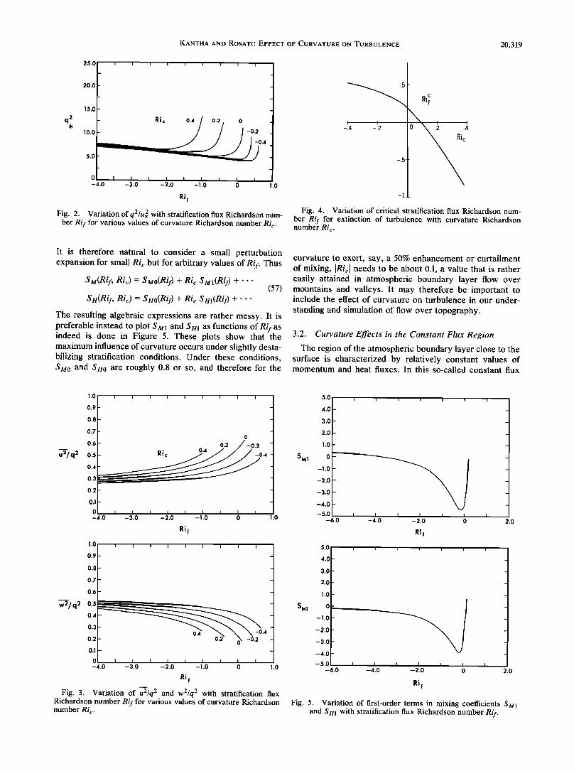
Figures 2 and 3 show the variations of q.(=q/u), u/q, and w/q, with Rif (v/q remains a constant) for various values of RIG.. It is important to note that unlike rotation [Kantha et al., 1989], curvature terms occur explicitly in the turbulence kinetic energy equation. Thus while rotation tends mainly to redistribute turbulence kinetic energy among its components, curvature tends to suppress or enhance turbulence production, somewhat akin to the effect of buoyancy on turbulence. One would therefore expect buoyancy and curvature effects to be more similar in some aspects than rotation and curvature effects, in general. Figure 4 shows a plot of the critical buoyancy Richardson number Rif for complete suppression of turbulence as a function of the curvature Richardson number Ric.

In geophysical flows, one is often concerned with the limit of strong stratification but relatively weak curvature effects.

KANTHA AND ROSATI' EFFECT OF CURVATURE ON TURBULENCE 20,319

q2 15.0J-

10.0

5.0

.

i i i I i i i i i

Ri c 0.4 o

o

-4.0 -3.0 -2.0 -1.o o 1.o

Ri f

Fig. 2. Variation of q2/u,2 with stratification flux Richardson number Rif for various values of curvature Richardson number Ric.

-.2 .2 .4 ß

-1

Fig. 4. Variation of critical stratification flux Richardson number Rif for extinction of turbulence with curvature Richardson number Ri c.

It is therefore natural to consider a small perturbation expansion for small Ric but for arbitrary values of Rif. Thus

Sm(Rif, Ric) = Smo(Rif) + Ric Sml(Rif) +'"

SH(Rif, Ric) = SHo(Rif) + Ric Sm(Rif) +'" (57)

The resulting algebraic expressions are rather messy. It is preferable instead to plot $2u• and S H1 as functions of Rif as indeed is done in Figure 5. These plots show that the maximum influence of curvature occurs under slightly destabilizing stratification conditions. Under these conditions, SMO and SH0 are roughly 0.8 or so, and therefore for the

curvature to exert, say, a 50% enhancement or curtailment of mixing, IRicl needs to be about 0.1, a value that is rather easily attained in atmospheric boundary layer flow over mountains and valleys. It may therefore be important to include the effect of curvature on turbulence in our under-

standing and simulation of flow over topography.

3.2. Curvature Effects in the Constant Flux Region

The region of the atmospheric boundary layer close to the surface is characterized by relatively constant values of momentum and heat fluxes. In this so-called constant flux

1.0 I I

0.9 -

0.8

0.7 _

o

0.61- 0.2 /-0.2 "/q 2 0.5 ' ' ,4

0.4

0.3

0.2

0'1 t 0 -4.0 -3.0 -2.0 -1.0 0

Rif

0.9 -

0.8 -

0.7 -

0.6 -

0.3 0.4 .,4

0.2 0.2 o N -0.2 0.1

0 I I I I I I I I I -4.0 -3.0 -2.0 -1.0 0 1.0

Ri f

Fig. 3. Variation of u2/q 2 and w2/q 2 with stratification flux Richardson number Rif for various values of curvature Richardson number Ri c.

SM1

SIll

5.0

4.0-

3.0-

2.0-

1.0-

0

-1.0

-2.0

-3.0 -

-4.0 -

-5.0 -6.0

I I I I I I I •

-4.0 -2.0 0

5.0

4.0

3.0

2.0

1.0

0

-1.0

-2.0

-3.0

-4.0

-5.0

Rit

-4.0 --2.0 0

2.0

, i i b.o 2.o

Rif

Fig. 5. Variation of first-order terms in mixing coefficients S M1 and Sm with stratification flux Richardson number Rif.


region, extending to perhaps 50 m above the surface, the momentum flux is constant to within 20% or so [see Monin and Yaglom, 1971] and the wind turning angle is within about 10 ø. Monin-Obukhov similarity laws pertaining to the profiles of velocity, temperature, and other quantities for the atmospheric constant flux region in the presence of stratification are rather well known [Monin and Yaglom, 1971]. Considerable observational [Businger et al., 1971] and modeling [Mellor, 1973; Lewellen and Teske, 1973] efforts have been expended in determining the form of these similarity functions. In fact, the widespread "popularity" of second moment closure techniques in geophysics can be attributed to the "successful" prediction of these Monin-Obukhov similarity functions in the early seventies [Mellor, 1973; Lewellen and Teske, 1973]. It is therefore natural to inquire how curvature affects Monin-Obukhov similarity and to what extent. To explore this aspect, we rescale (30) to (39) and (53), which yield after some manipulation

3Alq, [ ] 6A1

•--(qbm+•rc) Yl q,3 (•r+2•rc) -Cl(cbm-•-c)

[ 6A1 3A2•r

-2•rc •/•+ q,3 (qbm+•rc) q,3 + + (58)

3A2q, 6A• ] -qbH •/• q,3 (•r+2•rc) B2 6A2

q,3 CbH•' q,5- (Cbm + CbH + •'c)•'c (59) q,3_ B•(CbM- •'- •'c) (60)

where

q q, = -- (61a)

I ou CbM = -- -- (6lb)

u, 0z

lu, O© &u = (61c)

H Oz

1391H

•'- u* 3 (61d)

u, 1 + kxz (61e)

The quantities u, 2 (= -uw) and H (= - wO) denote the nearly constant kinematic momentum and heat fluxes in the con-

stant flux region. Also •/• = • (1 - 6A•/Bi) and I - kz. We note that (58)-(60) reduce to equation (42) of Mellor

[1973], when src - 0. Equations (58)-(60) can be solved for •bM, •b•, and q, by

the Newton-Raphson technique for arbitrary values of s r and sr•.. But before presenting these results, for future reference we will record the rescaled equations for turbulence energy components:

9.01 I I I I I I I I I I I I I/ I/ I /

8.0

7.0

6.0

•M ß ø'a ø'2 o 3.0 -0 2.O -0.2

-1.0 I I I I I I I I I I I I I I I / -6.0 -5.0 -4.0 -3.0 -2.0 -1.0 0 1.0 2.0

9.0

8.0

7.0

6.0

5.0

•H 4.o 3.0

2.0

-1.0

-6.0 -5.0 -4.0 -3.0 -2.0 -1.0 0 1.0 2.0

Fig. 6. Variation of Monin-Obukhov similarity functions qb M and qb H in the constant flux layer with stratification Monin-Obukhov similarity variable • for various values of curvature similarity variable •c.

6A1

3' • + q,3 (•b M + s r c) (62a)

3'1 (62b)

6Ai

3'• q,5-(st + 2src ) (62c) Figures (6)-(8) present &3•, &u, q,2, u2/q2, and w2/q 2 as functions of •r for various values of •r c. These plots display the strong influence (both stabilizing and de stabilizing effect) that strong curvature can exert in stratified flows. However, in most geophysical situations the parameter •r c is rather small (less than 0.03 or so), and interesting as the plots in Figures (6) to (8) are, it would be of interest to explore small perturbation expansions for 4•M and 4•u in terms of •rc:

4u(, 4u0(O + +'" (63a)

•Hb ?', b?'c): •H(b?') q- b?'c•H(b?') q-.-- (63b)

q*(g, gc) = q•(g) + gcq•(g) +''' (63c)

The governing equations yield

qbM0[(3'l -- Cl)q3,o - (6Al + 3A2)s r] - qbHo(3A2s r) =- q,o

3Al

(64a)


25.0

22.5

20.0

17.5

15.0

2 q, 12.5

10.0

7.5

5.0

2.5

o

0.4 0 0 I I I I I

-6.0 --5.0 -4.0 --3.0 --2.0 -1 .o o 1 .o 2.0

Fig. 7. Variation of q2/u,2 in the constant flux layer with stratification Monin-Obukhov similarity variable • for various values of curvature similarity variable •c.

q,0 qb/_/0[ylq3,0- (6A1 + B2)s r] = • (64b)

3A2

q3,0 = Bl(qb•40- s r) (64c) which are identical to equations (42) of Melior [ 1973] for zero curvature, and

[('y• - C•)q3,o - (6A1 + 3A2)sr]qbM1 - (3A20•m

+ 3(T, - C,)•moq}o-- = 24AlUm0 + (T1 - Ci)q•o + 3(2A1 + A2)• (65a)

1.0 I I I I I I I I I I I I I I I "'

_

_

.6

.5 0.4

.3

-

.1

0 I I I I I I I I I I I I I •0 • -6.0 -5.0 -4.0 -3.0 -2.0 -1.0 o 1.

1.o I I I I I I I I I I I I I I I

-; .

ß •'c 0.4 '

0 I I I I I I I I I i I 0 --i.O --41.0 --31.0 --2.0 --1.0 0 1.0 2.0

Fig. 8. Variation of u2/q 2 and w2/q 2 in the constant flux layer with stratification Monin-Obukhov similarity variable • for various values of curvature similarity variable •c.

20.0" I I

17.0 -

14.0 -

11.0 -

8.0-

•M'• •.o- 2.0-

-1.0 -

-4.0 -

-7.0 -

-10.0 I I -6.0 -5.0

I I I I I I I -4.0 -3.0 -2.0 -1.0

I i i i I !

_

I I I I I o 1 .o 2.o

5.0 i i i i i I i I

3.5-

2.0-

0.5-

-1.0-

-2.5-

-4.0-

-5.5-

-7.0-

-8.5

6. 0 -5.0 -4.0 -3.0 -2.0 -1 .o o

I

i I 1 .o 2.o

Fig. 9. Variation of first-order terms in Monin-Obukhov similarity functions, •bM1 and •bH1, in the constant flux layer with stratification Monin-Obukhov similarity variable •.

2q*ø 1 [ylq3,0- (6A1 + B2)sr]qbH1 + 3ylq2,0qbH0 --•22]q,1 = 6A2qbm0 + 6(2A1 + A2)qbH0 (65b)

- Blqbm! + 3q2,oql = B1 (65c)

Figures (9) and (10) show qb3•l, qb/-n, and q,1 as functions of s r. The maximum effect of curvature occurs very near neutral stratification and amounts to less than perhaps a few tens of percent on qb•u but significantly lesser on qb/_/. For neutrally stratified flows,

4)M-' 1 + (1 + 54A12B•-2/3)•' c (66a)

qb H = (3A2,Y1B•/3) -1

{ 6 } ß 1 + [2A1 + A2 + 371B•/3(A22 - A12)]•'c (66b) YlB1

Thus qb•u = 1 + 8.02Src for neutrally stratified flows. Once again, assuming Src can be about 0.02 in the constant flux region, qb•u can change by about 15% or so, a small though nonnegligible amount.

Finally, the relative importance of stratification and curvature in the constant flux region is governed by the ratio

Src L IIc .... (67)

• Lc


q*l

20.0

17.0

14.0

11.0

8.0

5.0

2.0

-1.0

I I I I I I I I

_

-4.0-

-7.0-

--10.0 I I I I I I -6.0 -5.0 -4.0 -3.0

.

I I I [ I I I

-2.0 -1.0 0 10 2.0

Fig. 10. Variation of first-order term q, 1 in the constant flux layer with stratification Monin-Obukhov similarity variable •.

where L = u,3/kl3gH is the Monin-Obukhov length scale that indicates the relative magnitude of buoyancy production vis-h-vis shear production in the surface layer, while

l+kxzU R U Lc - (68)

kkx u, k u,

is the corresponding curvature length scale, essentially a modified radius of curvature.

4. CURVATURE EFFECTS IN FI•OW OVER TOPOGRAPHY

In this section, we will proceed to incorporate curvature effects in simulations of flow over two-dimensional moun-

tains and valleys to illustrate the application of the model to geophysical flows and the utility of the turbulence closure incorporating curvature effects. These simulations serve rather well the limited purpose of demonstrating the simplicity of incorporating curvature effects in atmospheric boundary layer calculations. The investigation of more realistic topography is desirable but beyond the scope of this paper.

1

We will use a level 2• model consisting of (15), (16), (45), and (46). We will, however, ignore curvature terms in turbulence diffusion in (15) and (16). This is inconsequential because the diffusion terms are in most cases rather small anyway. For convenience, we will also align the local coordinate in the local direction of flow when calculating shear production in these equations, which can then be written as

Dt (q • qlSq • (q = 2q!S•4 (1 - Ric) 3

q - 2 qlSHj•/Oz -- 2 (69)

B•l

(q2/) _ Oz qlSl • (q2/) E•ql2S• (1 Ric)

- EiE3ql2SuBaOz-• 1 + E2 • (70) We have used tildes over the velocity to remind the reader

that the coordinate is aligned in the local flow direction so that the total shear is O U/Oz. The flow then does not "feel"

the curvature in the direction perpendicular to the mean flow direction and the resulting expressions are hr simpler than those that would result when the coordinates are aligned in

D

Dt

an arbitrary direction. It is important to stress that there is no loss of generality at all in adopting this particular proce- dure in calculating the turbulence properties. Note also that in (69) and (70), Ri c (equation (47)) is also based on U.

Equations (69) and (70) along with (45) and (46) constitute 1

the level 2• equations for calculating the properties of turbulence in the flow of stratified fluids over curved sur-

faces in geophysical context. These equations can be solved by standard techniques, along with the momentum, continu- ity, and heat balance equations to simulate flow over topography. Since we are mainly interested in the influence of curvature on such flows, we will not describe the details of the simulation. Instead, we will briefly summarize the conditions of two identical twin experiments, with and without curvature effects, of a flow over a two-dimensional mountain and a two-dimensional valley.

The model uses Bousinesq and hydrostatic approximations as well as dry perfect gas relation for the atmosphere. The grid resolution is 2 km in the horizontal, and the domain is 160 km wide. There are 60 levels in the vertical with a

resolution of 250 m in the upper regions but a maximum of 10 m immediately adjacent to the ground so as to resolve the lower layers of the atmosphere. The model uses topograph- ically conformal coordinate (o-coordinate) in the vertical and mode splitting for efficiency. But the most important feature of the model is the inclusion of second-moment closure of

turbulence field, so that the turbulent mixing in the boundary layer and the wave-breaking regions aloft are parameterized properly and not in an ad-hoc fashion. Since intense regions of turbulence aloft are a prominent feature of high mountain drag situations, it is our hope that the flow can be better simulated by a model such as this. Finally both the atmospheric boundary layer and rotational effects on the flow are retained explicitly in the model.

Both the mountain and the valley have a vertical scale H of 1 km and a horizontal scale (effective half-width W) of 10 km, and are in the shape of a witch of Agnesi curve. A mountain of this shape has a moderate concave shape over most of the width, with a stronger convex shape near the center. The atmosphere is stably stratified, with potential temperature increasing linearly with height. The buoyancy frequency is 0.02 s -1 , and the flow is from the right to the left at 10 m s -[ . The relevant nondimensional parameters are

NH fW NW Fi = • = 2 Rol- • = 0.1 FH = • = 20

U U U

where Fl is the inverse Froude number, Ro• is the inverse Rossby number, and F H is the hydrostatic parameter. The value of F• is slightly larger than the value at which the waves break and the high drag regime results. F• is sufficiently large so that the hydrostatic approximation holds well. The inverse Rossby number is small but not small enough for rotational effects to be ignored in the momentum equations. The values chosen are typical of the high mountain wave drag regime. The calculations are carried out until steady state conditions are attained.

Figure 11 compares the potential temperature distribution with and without curvature effects on turbulence. The most

noteworthy aspect is the absence of significant wave activity above the breaking region, when curvature effects are included. Although the drag exerted by the mountain on the flow changes by a small amount, the absence of wave


7 i

6

5

4

i I i I '. • i i i ! i i i i 7 i i i i i I i i i i i i I I I

i

0 I I I I I I I I I I I I I I I

7

3

2

1

o o

i i i i , i , i I I i , i , i

-.. .

20 40 60 80 100 120 140 160 0 j I , I I I I 0 2• ' 40 60 810 I I I I I •o •o •,•o •o

DISTANCE (km) DISTANCE (km)

Fig. 11. Distribution of potential temperature over a mountain (top) without and (bottom) with curvature effects on turbulence. The contour interval is 2øK. The flow is from right to left. Note the hydraulic jump in the lee of the mountain in both cases and residual wave activity aloft in the former.

Fig. 12. Distribution of turbulence kinetic energy over the mountain (top) without and (bottom) with curvature effects on turbulence. The contour interval is 0.1 m 2 s -2. The flow is from right to left. Note the hydraulic jump and the associated strong turbulence near the ground, in addition to the turbulence in the wave breaking region aloft, in the lee of the mountain in both cases.

activity aloft is more significant, and this could be potentially important for the dynamics of the middle atmosphere. Figure 12 compares the turbulence kinetic energy distribution in the two cases. The differences are well within 10%. Both cases

show a strong turbulent region produced by the hydraulic jump to the lee of the mountain. Strong turbulence is also evident over the leeward slope due to intense shear of the flow plunging down the leeward slope and aloft due to wave breaking. However, the turbulence in the boundary layer appears to be rather small compared with those in these intensely turbulent regions. Figures 13 and 14 show the cross- slope and along-slope wind velocity distributions. Once again, the significantly lesser wave activity aloft is evident in cross- slope wind distribution. Both cases, however, show strong downslope winds characteristic of the high mountain drag regime. The along-slope winds are strong in the region ahead of the mountain, indicating some blocking effects. They are also strong in the breaking region aloft on the leeward side. Values of curvature Richardson number (not shown) as high as 0.1 and as low as -0.3 occur in some localized regions, but typical values range between -0.1 to +0.1.

Figures 15 and 16 show the corresponding distributions of potential temperature and turbulence kinetic energy for an identical flow over a valley. It immediately becomes appar- ent that valley flows differ significantly from mountain flows. The asymmetry is rather sinking. There is some wave breaking aloft, but strong turbulence is confined to the upwind side of the valley. There is litle wave activity aloft with or without curvature effects compared with that over a mountain of similar shape and size. The turbulence created aloft is not as intense as in the case of a flow over a mountain. Curvature

effects tend to reduce these intensities even further, as can be seen from Figure 16. They also appear to suppress wave

activity aloft as can be seen from the distribution of cross-slope winds in Figure 17. Strong cross-slope winds are confined to the vicinity of the underlying surface (Figure 18).

From these results it is clear that curvature effects, if not overwhelmingly important, are not negligible. Some moderate influence is surely present in flow over topographic changes. An encouraging aspect, however, is that it is rather simple to include it with little or no influence on model structure and economy. Since curvature effects depend clearly on the details of the topography, their influence will not necessarily be the same for mountains (or valleys) of equivalent size, unless they are also of equivalent shape. In any case, a mesoscale model of flow over a rugged terrain that includes not only the turbulence'Caused by wave breaking activity but the effect of curvature on the resulting turbulence as well can be readily constructed. Such a model should further our understanding of topographic effects on the atmosphere.

A particular lesson from these simulations is that the details of the topography bel øw are important in at least as far as the influence of the topography on the lower and perhaps the middle atmosphere as well. An interesting corollary is that it may not be possible to accurately simulate all topographic effects in general circulation models, if there is not sufficient resolution in both the horizontal and vertical directions to resolve the regions in the immediate vicinity of the terrain below that are affected by topographic effects. Envelope orog- raphy can to some extent account for blocking effects of mountains, but an accurate simulation of the topographic drag on the atmosphere may still be elusive. Curvature effects of topography, which depend so strongly on the details of topography below, would be another complicating factor in this picture.

20,324 KANTHA AND ROSATI'. EFFECT OF CURVATURE ON TURBULENCE

...-. 5 E

2 • •,• _

1

0! ! I I, I I I I _1• I _ I •._ I I I I 0 20 40 60 80 100 120 140 160

DISTANCE (km) ' I

Fig. 13. Distribution of velocity component across the mountain (top) without and (bottom) with curvature effects on turbulence. The contour interval is 1 m s ]. The flow is from right to left. Note the hydraulic jump in the lee of the mountain in both cases and residual wave activity aloft in the former.

I I I I I I I I I I I I I I I

8•

7

6-

5

4-

3'

2

1-

0 0

I I I I I I I I I I I I I I I 20 40 60 80 100 120 140 160

DISTANCE (km)

Fig. 15. Distribution of potential temperature over a valley (top) without and (bottom) with curvature effects on turbulence. The contour interval is 2øK. The flow is from right to left. Note the wave activity upstream of the valley in both cases.

5. CONCLUDING REMARKS

It is clear from this study that curvature exerts a nonnegligible influence on small-scale turbulence and vertical mixing in stratified fluids. It is of potential importance in the study of flows over mountains and sea mounts in the

6

0 I I I I I I I I I I I I I I I 0 20 40 60 80 100' 120 140 160

DISTANCE (km)

Fig. 14. Distribution of velocity component parallel to the mountain (top) without and (bottom) with curvature effects on turbulence. The contour interval is 1 ms-]. Note strong velocities upstream of the mountain in both cases.

geophysical context. Unfortunately, geophysicists have paid little attention to these matters, and there are few observational data on the combined effects of curvature and strati-

fication on small-scale turbulence and mixing in geophysical

i i i i i i i i i i i

[ i i i

i i i I

I I I [ I I I I I

_

3-

0 i 410 i i I i i 0 210 i 60 80 11•10 i

-

i i I I i i

120 1 0 160

DISTANCE (km)

Fig. 16. Distribution of turbulence kinetic energy over the valley (top) without and (bottom) with curvature effects on turbulence. The contour interval is 0.1 m 2 s -2. The flow is from right to left. Note the strong turbulence aloft upstream of the valley, especially in the former case.


I i I I I I I I I I I I I I I

6

'!- 2

1

O,

i i i • ! _

I I I I I I I I I I I • I I I 20 40 60 80 100 1 0 140 160

DISTANCE (km)

Fig. 17. Distribution of velocity component across the valley (top) without and (bottom) with curvature effects on turbulence. The contour interval is 1 m s-1. The flow is from right to left.

or laboratory boundary layers. Although an excellent start has been made in investigating curvature effects on geophysical boundary layers [Zeman and Jensen, 1988], the investigation considered only the neutrally stratified case. Similar investigations on flow over topography under stratification,

both stable and unstable, would be of great help in furthering our understanding of stratified flow over topography.

APPENDIX A: IMPLICIT CURVATURE TERMS

We have ignored implicit terms involving curvature and retained only the explicit terms in the equations for Reynolds stresses and turbulent heat fluxes. The implicit terms are terms that could be included in the modeling of pressure strain and pressure-temperature gradient covariances to account for the possible influence of curvature (or rotation) on these covariances. Zeman and Tennekes [1975] extended the Rotta model for the pressure strain covariance term to include the effect of rotation by invoking tensorial invariance principles. The resulting form for the implicit rotational terms is identical to that of the explicit rotational terms, and the consequence of retaining the implicit terms appears to be that these terms tend to counteract the explicit terms and thus decrease the influence of rotation on turbulence

stresses.

Recently, Zeman and Jensen [1988] have invoked a loose anology between rotation and curvature to suggest a possible form for the implicit curvature terms in the turbulence stress equations. Once again, they are similar in form to the explicit curvature terms and they tend to counteract the latter. With the coordinate system aligned such that the horizontal component of the velocity vector is along the x• axis, the implicit terms take the form [Zeman and Jensen, 1988]

2a 2C[ e i2qUqlljq- Ej2qUqUiq- E i21U llljq- e j21 u lUi q- • u--• ij]

so that (30)-(36) become, in the absence of rotation and buoyancy terms,

8

7

6-

5-

4-

3-

2- _

1-

0

i


6-

5-

4

3-

2-

1-

0 0

I I I I I I I I I I I I I I 20 40 60 80 100 120 140 160

DISTANCE (km}

Fig. 18. Distribution of velocity component parallel to the valley (top) without and (bottom) with curvature effects on turbulence. The contour interval is 1 m s-•. Note strong shear downstream of the valley in both cases.

u 2=• 1 .... u'-• '•+ 1- a 3 B•J q Oz • 2 l+kxz

(A1)

7=0 5- -. B 1 J q -• a2 1 + kxz

w2=-• - 1 ---' +•u• 2---a2 B•/ q 3 1

(A2)

kxU 'J + kxz

(A3)

Uv=0 (A4)

• + (1 - 2a2)(w 2- 2u 2) q Oz 1 + kxz

21ou ) - C•q [• •'• 1 + kxz' (A5)

vw = 0 (A6)

Equations (A1)-(A6), along with the use of the local equilibrium form of the turbulence kinetic energy equation (53) give rise to


I -5

1.2

1.0

0.8

0.6 S M

=0 0.• -4 -3 -2 -1 0 0.1 0.2

Ric

Fig. A1. Variation of momentum mixing coefficient S M with curvature Richardson number Ri c for two cases a2 = 0 and a2 = 0.3; a2 is the implicit curvature parameter. The extinction value of Ric (of 0.08 or so) is more realistic for a2 of nearly zero.

6A1 ) SM- A1 1 3C• (1 - Ric) - 72A• Ric(1 + Ric) B1 (1 -Ric)

[ // 6Al• 6A12 Ric

+ 2a2[A,•, )Ric+ B1 B1 (1 -Ric)

ß (11 + 25Ric - 26a 2 Ric)] (A7)

The value of a2 is not known with certainty. Zeman and Jensen [1988] suggest a value of about 0.3, and they cite field observations over Askervein Hill in Scotland that appear to support a value of this magnitude. Figure A1 shows SM plotted against Ri c for a2 = 0 and a2 = 0.3. It is clear from this plot that inclusion of implicit terms tends to ameliorate curvature effects. For example, the magnitude of Richardson number Ri c at which the turbulence is extinguished increases substantially for a2 = 0.3. However, it is not at all clear whether this high value of a2 is justified and even whether the form of these terms should be what Zeman and Jensen

[1988] hypothesized by using a rather loose anology between curvature and rotation. Their extension to the Rotta [1951] model lacks concrete support, although the suggested form is certainly plausible. As for the value of a2, it should probably be substantially smaller, since a model by Melior [1975], which is similar to the model discussed here and which ignored implicit terms, yields quite good agreement for the extinction curvature Richardson number with labo-

ratory observations of turbulent boundary layer on a convex wall by So and Mellor [1973]. Although Zeman and Jensen [1988] suggest that the above cited field data supports their model for the implicit terms, it is not clear whether the model is valid for the very strong curvature of the Askervein Hill. Even if it were, the model-predicted extinction Ri c would substantially differ from the observations of So and Mellor [1973], which suggests a value near zero for a2. So we regard

the question of implicit curvature terms as an unresolved issue and for simplicity ignore all implicit terms in the turbulence equations. The reader should remember that the curvature effects are therefore somewhat overestimated

here; we suspect the overestimation is small but we cannot say how much.

APPENDIX B' EFFECTS OF STRATIFICATION IN FLOWS

AFFECTED BY CURVATURE

We looked at the combined effects of stratification and

curvature on turbulence, mainly from the point of view of geophysical flows, particularly the atmospheric boundary layer. We therefore regarded stratification as the primary and dominant effect, but curvature was considered to be a secondary influence. It is, however, instructive to inquire what the effect of stratification would be in flows affected by curvature, instead of exploring the effect of curvature in stratified flows. It should be noted that neutrally stratified flows over curved surfaces are important in engineering, and considerable effort has been expended in modeling such flc•ws [see Bradshaw, 1973; Mellor, 1975; So, 1975]. Al- though gravitational stratification is rather negligible in engineering devices, it is nevertheless interesting to study the effect of stratification on flows over curved surfaces.

The governing equations (55) and (56) can also be solved

for SM and S//as functions of Ric for various values of Rif; the results are shown in Figure B1. A noteworthy aspect of Figure B 1 is the strong suppression of turbulent mixing at sufficiently large de stabilizing values of Ri c. This is some-

2.0

1.8

1.6

1.4

1.2

S• 1.o 0.8

0.6

0.4

0.2

0

S H

_ --

--2.0 --1.5 --1.0 -0.5 0 0.5 1.0 1.5 2.0

8.0

7.2

6.4

5.6

4.8

4.0

3.2

Ric


__ __

1.61 ' 0.8

0 I I I --2.0 -1.5 --1.0 -0.5 0 0.5 1.0 1.5 2.0

Ric

Fig. B 1. Variation of mixing coefficients S M and S H with curvature Richardson number Ri c for various values of stratification flux Richardson number Rif.


2

25.0 •

20.0

15.0

10.0

_

5.0-

_

0 • • -2.0 -1.5

I I I I I I I I I I I I

-4•)

2•)

Ril o

0.2

i I 1.5 2.0 -I .0 -0.5 0 0.5 1.0

Ric

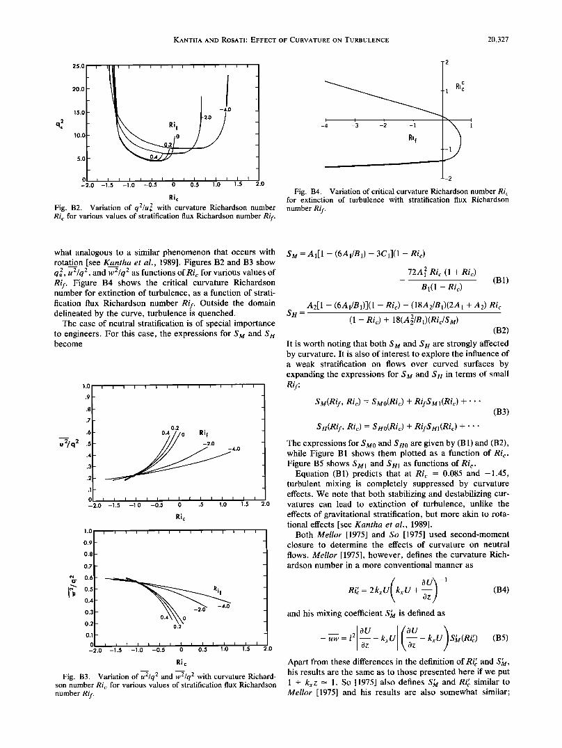
Fig. B2. Variation of q2/u,2 with curvature Richardson number Ri c for various values of stratification flux Richardson number Rif.

-2

-4 -3 -2 -1 N,• 1 ß

-2

Fig. B4. Variation of critical curvature Richardson number Ri•. for extinction of turbulence with stratification flux Richardson

number Rif.

what analogous to a similar phenomenon that occurs with rotation [see Kantha et al., 1989]. Figures B2 and B3 show q,2, u2/q2, and w2/q 2 as functions of Ric for various values of Rif. Figure B4 shows the critical curvature Richardson number for extinction of turbulence, as a function of strati-

fication flux Richardson number Rif. Outside the domain delineated by the curve, turbulence is quenched.

The case of neutral stratification is of special importance to engineers. For this case, the expressions for S M and S n become

1.0

.9

.8

.7

.6

'•q2 .5 .4

.3

.2


__

__

1.0

0.9

0.8

0.7

0.6

0.4

0.3

0.2

0.1

0

- o.•,//o Rif - _

-- .

-4.0

_

_

.1 - -

0 I I I I I I I I I I I I I i ! --2.0 -1.5 --1.0 --0.5 0 .5 1.0 15 •.0

Ric


--

-

-2.0 -1.5 -1.0 -0.5 0 0.5 1.0 1.5 2.0

Ric

Fig. B3. Variation of u2/q 2 and w2/q 2 with curvature Richard- son number Ri c for various values of stratification flux Richardson number Rif.

SM = Al[1 - (6A1/B1) - 3C1](1 - Ric)

72A • Ric (1 + Ric) ml(1 - gic)

(B1)

A211 - (6AliBi)](1 - Ric) - (18A2/B1)(2A1 + A2) Ric SH =

(1 - Ric) + 18(A22/B1)(Ric/SM) (B2)

It is worth noting that both S•4 and Sn are strongly affected by curvature. It is also of interest to explore the influence of a weak stratification on flows over curved surfaces by expanding the expressions for S•4 and Sn in terms of small

Sm(Rif, Ric) = Smo(Ric) + RifSml(Ric) +''' (B3)

SH(Rif, Ric) = SHo(Ric) + RifSm(Ric) +"'

The expressions for S•40 and Sn0 are given by (B 1) and (B2), while Figure B1 shows them plotted as a function of Ric. Figure B5 shows S•41 and Sm as functions of Ric.

Equation (B1) predicts that at Ri• = 0.085 and -1.45, turbulent mixing is completely suppressed by curvature effects. We note that both stabilizing and destabilizing curvatures can lead to extinction of turbulence, unlike the effects of gravitational stratification, but more akin to rotational effects [see Kantha et al., 1989].

Both Me#or [1975] and So [1975] used second-moment closure to determine the effects of curvature on neutral

flows. Mellor [1975], however, defines the curvature Rich- ardson number in a more conventional manner as

Ri3 = 2kxU kxU + (B4)

and his mixing coefficient Sh is defined as

.... kxU -- kxU S•(Rl3) (B5) Oz

Apart from these differences in the definition of Ri3 and S•, his results are the same as to those presented here if we put 1 + k•z • 1. So [1975] also defines S• and Ri• similar to Mellor [1975] and his results are also somewhat similar;


SM1

SIll

2.0

-3.0 -2.0

2.0

-3.0 -2.0

I I I I I I I I I I I

i I i i i i I i I i i -1.5 -1.0 -.5 0 .5

Ri c

I I I I I I I I I I I

i I I I I I I i i i i -1.5 -1.0 -0.5 0 0.5

Ri c

1.0

a form identical to equation (12) of So [ 1975], if we make use of (B7) and the fact that So puts C1 = 0. Making use of (B4) and (B5), (B8) can be written as

' I -2/3 S• = 1 - 32A•2B1 -

2/3

(B9)

an expression identical to that of Mellor [1975]. In the limit of neutral stratification, (58)-(60) for the

constant flux region can be written as

•= ((•M + •c) •1 .... C ((•M-- •c) 3 A lq, q3, •

-2•'c Yl + q3, (•bM+ •'c)

1 I12Al•'c]6A2 3A2q,- •H ')/1 c q3, q3, + q3, = ;c)

(B10)

(Bll)

(B12)

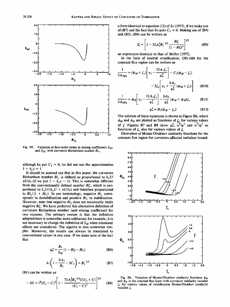
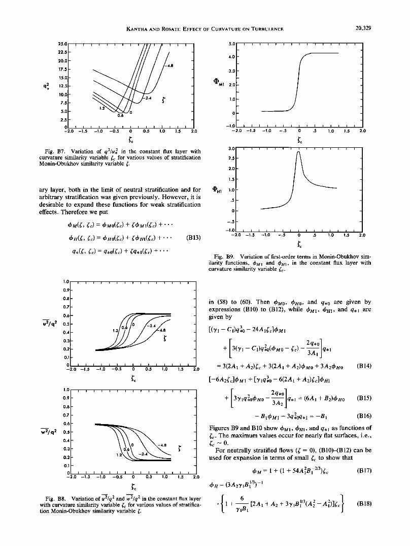
The solution of these equations is shown in Figure B6, where •b•/and •bn are plotted as functions of •c for various values of •. Figures B7 and B8 show q.•, u2/q 2 and w2/q 2 as functions of •c also for various values of •.

Derivation of Monin-Obukhov similarity functions for the constant flux region for curvature-affected turbulent bound-

Fig. B5. Variation of first-order terms in mixing coefficients S Mi and S HI with curvature Richardson number Ric.

although he put C• = 0, he did not use the approximation l +kxz-•l.

It should be pointed out that in this paper, the curvature Richardson number Ri c is defined as proportional to kxU/ OU/Oz (if we put 1 + kxz "• 1). This is somewhat different from the conventionally defined number Ri•, which is proportional to kxU/(kxU + OU/Oz) and therefore proportional to Ric/(1 + Ric). In our terminology, negative Ric corre- sponds to destabilization and positive Ri c to stabilization. However, note that negative Ric does not necessarily imply negative Ri•. We have preferred this alternative definition of curvature Richardson number (and mixing coefficient) for two reasons. The primary reason is that the definition adopted here is somewhat more utilitarian; for example, it is not necessary to change the definition of SM when rotational effects are considered. The algebra is also somewhat simpler. Moreover, the results can always be translated to conventional values in any case. If we make note of the fact that

B1 = • (1 - Rif- Ric) q,4 SM

a,(1

(B6)

(B 1) can be written as

- uw = 12(Uz - C)2[ 1 -

6A1 3C1) = B• -1/3 (B7) B1

2 -2/3 13/2 72A1Bl C(U z + C)

(U• - C) 2 (B8)

9.0

8.0

7.0

6.0

5.0

CI) M 4.0 3.0

2.0

1.0 - r'

-1.0 • I I I •) ' 01.5 ' 1. 1. 2.0 -2.0 -1.5 -110 -d. 5 • I0 ' '5 '

(I) H

5.0 I I I I I I I I I I i I I I !

4.0 -

3.0-

2.0-

1.0-

0-

i i • i 015 , -1'02.0 -1.5 -1'.0 - .

1.2

0.6

0

-2.4

-4.8

I I I I I I I I

0 0.5 1.0 1.5 2.0

Fig. B6. Variation of Monin-Obukhov similarity functions qbM and qbH in the constant flux layer with curvature similarity variable •c for various values of stratification Monin-Obukhov similarity variable •.


25.0

22.5

20.0

17.5

15.0

2 12..5 q. 10.0

7.5

5.0

2.5

0 -2.0 -1.5

-- _


-1.0 -0.5 0 0.5 1.0 1.5 2.0

Fig. B7. Variation of q2/u,2 in the constant flux layer with curvature similarity variable •c for various values of stratification Monin-Obukhov similarity variable •'.

ary layer, both in the limit of neutral stratification and for arbitrary stratification was given previously. However, it is desirable to expand these functions for weak stratification effects. Therefore we put

+ +"'

•bu(sr, Src)= •buo(src) + sr•bm(•'c) +... (B13)

= e,0(c) + +'"

5.0

4.0

3.0

C•M1 2.0

1.0

-1.0 --2.0 -1.5

CI)H1

2.5-

2.0-

1.5-

1.0-

.5 -

0-

-1.0 I • -2.0 -1.5

I I I 15 I I I I I I -1.0 --. 0 .5 1.0

re i

i i i i i i i i i i i i -1.0 -.5 0 .5 1.0 1.5

t"c

2.0

Fig. B9. Variation of first-order terms in Monin-Obukhov similarity functions, •bM1 and •bH], in the constant flux layer with curvature similarity variable •'c-

1.0

0.9

0.8

0.7

0.6- __

u2/q 2 0.5 - 0.4-

w2/q 2

0.3-

0.2-

0.1-

0 I I -2.O -1.5

0.9-

0.8-

0.7-

0.6-

0.5-

0.4-

0.3-

0.2-

0.1-

CI I I -2.O -1 ..5

I I i i I i i i i i I i i

_

I i i I I I i i i I i I -1.0 -0.5 0 0.5 1.0 1.5

I I I I I I I I I I I I I

_

I I I I I I I I I I I I I -1.0 --0.5 0 0.5 1.0 1.5 2.0

Fig. B8. Variation of u2/q 2 and w2/q 2 in the constant flux layer with curvature similarity variable •c for various values of stratification Monin-Obukhov similarity variable •'.

in (58) to (60). Then •b/u0, •bu0, and q,0 are given by expressions (B10) to (B12), while •bM1, •bH1, and q,1 are given by

[('Yl - C1)q3,o - 24Al•'c]qbM1

2q,o] + 3(3,1- Ci)q2,o(&MO- •'c)- 3Ai/q*l = 3(2A1 + A2)•' c -Jr 3(2A1 + A2)qbM0 + 3A2qbH0 (B14)

[-6A2•'c]qbmi + [Tlq3,o - 6(2A1 + A2)•'c]qbHi

2q,o] + 3'y,q2,o•bHo--•2-2]q,, = (6A, + B2)•bHo (B15) - Biqbmi + 3q,2oq,1 = -B1 (B16)

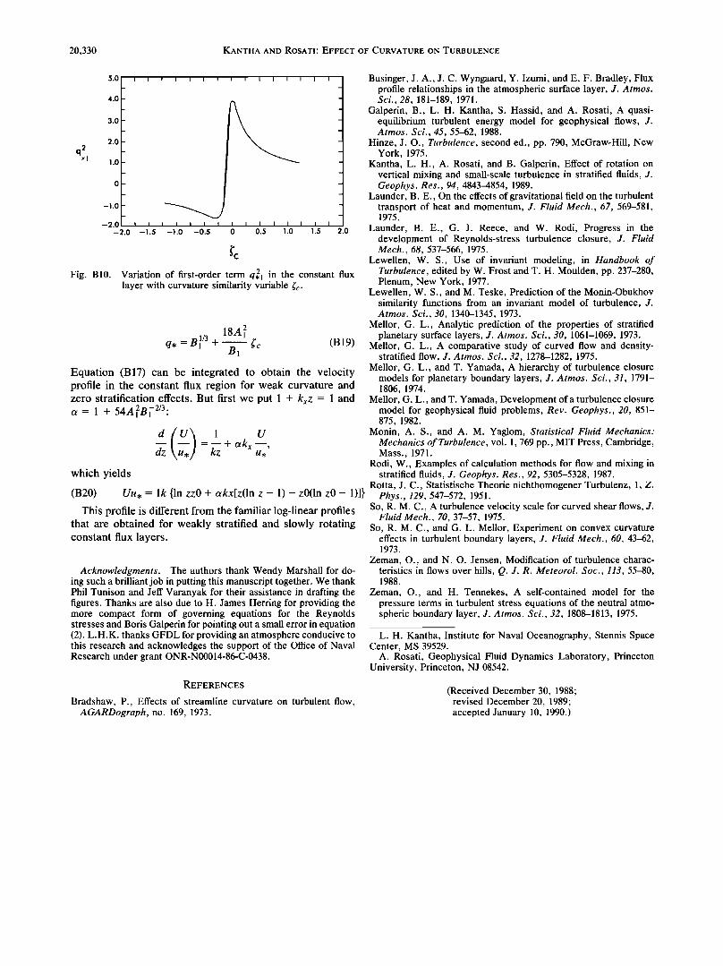
Figures B9 and B10 show •bM], •bm, and q,1 as functions of •c- The maximum values occur for nearly flat surfaces, i.e.,

For neutrally stratified flows (s r = 0), (B10)-(B12) can be used for expansion in terms of small sr½ to show that

2 2/3 •bM = 1 + (1 + 54AiB•- )•'c (B17)

qbH = (3A2'Y1B•/3) -1

6 ß 1+• 3,•B• ß -• 1/3,,• 2 } [2A1 + A2 + 3Ylt•l •,•t 2 -A12)]•'c (B18)


q2

5.0 • • _

4.0-

_

3.0- _

2.0- _

1.o-

_

0-

_

-1.0 - _

-2.0 I • -2.0 -1.5 1.5 2.0 -1.0 -0.5 0 0.5 1.0

Fig. B10. Variation of first-order term q,21 in the constant flux layer with curvature similarity variable •'c.

18A12 q, = B •/3 -t- • •'c (B 19)

B1

Equation (B17) can be integrated to obtain the velocity profile in the constant flux region for weak curvature and zero stratification effects. But first we put 1 + kxz = 1 and a = 1 + 54A12B• -2/3'

• = • + akx •, dz kz u.

which yields

(B20) Uu, = lk {In zzO + akx[z(ln z - 1) - z0(ln z0- 1)]}

This profile is different from the familiar log-linear profiles that are obtained for weakly stratified and slowly rotating constant flux layers.

Acknowledgments. The authors thank Wendy Marshall for do- ing such a brilliant job in putting this manuscript together. We thank Phil Tunison and Jeff Varanyak for their assistance in drafting the figures. Thanks are also due to H. James Herring for providing the more compact form of governing equations for the Reynolds stresses and Boris Galperin for pointing out a small error in equation (2). L.H.K. thanks GFDL for providing an atmosphere conducive to this research and acknowledges the support of the Office of Naval Research under grant ONRoN00014-86-C-0438.

REFERENCES

Bradshaw, P., Effects of streamline curvature on turbulent flow, AGARDograph, no. 169, 1973.

Businger, J. A., J. C. Wyngaard, Y. Izumi, and E. F. Bradley, Flux profile relationships in the atmospheric surface layer, J. Atmos. Sci., 28, 181-189, 1971.

Galperin, B., L. H. Kantha, S. Hassid, and A. Rosati, A quasi- equilibrium turbulent energy model for geophysical flows, J. Atmos. Sci., 45, 55-62, 1988.

Hinze, J. O., Turbulence, second ed., pp. 790, McGraw-Hill, New York, 1975.

Kantha, L. H., A. Rosati, and B. Galperin, Effect of rotation on vertical mixing and small-scale turbulence in stratified fluids, J. Geophys. Res., 94, 4843-4854, 1989.

Launder, B. E., On the effects of gravitational field on the turbulent transport of heat and momentum, J. Fluid Mech., 67, 569-581, 1975.

Launder, B. E., G. J. Reece, and W. Rodi, Progress in the development of Reynolds-stress turbulence closure, J. Fluid Mech., 68, 537-566, 1975.

Lewellen, W. S., Use of invariant modeling, in Handbook of Turbulence, edited by W. Frost and T. H. Moulden, pp. 237-280, Plenum, New York, 1977.

Lewellen, W. S., and M. Teske, Prediction of the Monin-Obukhov similarity functions from an invariant model of turbulence, J. Atmos. Sci., 30, 1340-1345, 1973.

Mellor, G. L., Analytic prediction of the properties of stratified planetary surface layers, J. Atmos. Sci., 30, 1061-1069, 1973.

Mellor, G. L., A comparative study of curved flow and density- stratified flow, J. Atmos. Sci., 32, 1278-1282, 1975.

Mellor, G. L., and T. Yamada, A hierarchy of turbulence closure models for planetary boundary layers, J. Atmos. Sci., 31, 1791- 1806, 1974.

Mellor, G. L., and T. Yamada, Development of a turbulence closure model for geophysical fluid problems, Rev. Geophys., 20, 851- 875, 1982.

Monin, A. S., and A.M. Yaglom, Statistical Fluid Mechanics: Mechanics of Turbulence, vol. 1,769 pp., MIT Press, Cambridge, Mass., 1971.

Rodi, W., Examples of calculation methods for flow and mixing in stratified fluids, J. Geophys. Res., 92, 5305-5328, 1987.

Rotta, J. C., Statistische Theorie nichthomogener Turbulenz, 1, Z. Phys., 129, 547-572, 1951.

So, R. M. C., A turbulence velocity scale for curved shear flows, J. Fluid Mech., 70, 37-57, 1975.

So, R. M. C., and G. L. Mellor, Experiment on convex curvature effects in turbulent boundary layers, J. Fluid Mech., 60, 43-62, 1973.

Zeman, O., and N. O. Jensen, Modification of turbulence charac- teristics in flows over hills, Q. J. R. Meteorol. Soc., 113, 55-80, 1988.

Zeman, O., and H. Tennekes, A self-contained model for the pressure terms in turbulent stress equations of the neutral atmospheric boundary layer, J. Atmos. Sci., 32, 1808-1813, 1975.

L. H. Kantha, Institute for Naval Oceanography, Stennis Space Center, MS 39529.

A. Rosati, Geophysical Fluid Dynamics Laboratory, Princeton University, Princeton, NJ 08542.

(Received December 30, 1988' revised December 20, 1989; accepted January 10, 1990.)

the effect of curvature on turbulence in stratified fluids · the effect of curvature on turbulence...

Documents