chapter 1 the unconditional linear latent curve model€¦ · the unconditional linear latent curve...

Chapter1 TheUnconditionalLinearLatentCurveModel

1.1 Introduction and Organization of the Workshop ........................................................................ 1‐3

1.2 Defining a Latent Growth Curve .................................................................................................. 1‐9

1.3 Latent Growth Curves as a Confirmatory Factor Model ........................................................... 1‐17

1.4 Thinking More Closely About Time ........................................................................................... 1‐35

1.5 Demonstration: Linear Trajectories of Negative Affect ............................................................ 1‐41

Adolescent and Family Development Project ...................................................................... 1‐43

Examining Descriptive Statistics ........................................................................................... 1‐43

Intercept‐only LCM, Heteroscedastic Residuals ................................................................... 1‐48

Intercept and Linear Slope LCM, Heteroscedastic Residuals ............................................... 1‐50

Intercept and Linear Slope LCM, Homoscedastic Residuals ................................................. 1‐52

1‐2 |Chapter 1 The Unconditional Linear Latent Curve Model

Copyright © 2015 Curran‐Bauer Analytics, LLC

1.1 Introduction and Organization of the Workshop | 1‐3


1.1 IntroductionandOrganizationoftheWorkshop

Objectives Provide a brief overview of the latent curve model (LCM)

Present recent exemplar uses of the LCM in practice

Describe the organization of the next three days

What is the Latent Curve Model? Latent Curve Model (LCM) is a form of structural equation

model (SEM) for the analysis of repeated measures (RMs) data

Uses latent factors to infer existence of unobserved growth trajectories based on set of observed RMs

Model no change, linear, quadratic, piecewise, etc.

Include one or more time-invariant predictors e.g., ethnicity, biological sex, country of origin, etc.

Include one or more time-varying predictors e.g., emotions, onset of diagnosis, marriage, arrest, etc.

Test interactions among time-invariant, time-varying, or both



What is the Latent Curve Model? Estimate growth in two or more constructs at once

multivariate latent curve model

Test mediating and moderating effects mediators of predictors of growth

growth as mediators in prediction of one or more distal outcomes

Test observed group heterogeneity multiple group analysis for gender, ethnicity, treatment group, etc.

Explore unobserved group heterogeneity growth mixture modeling to identify two or more latent subgroups

A non‐exhaustive sampling of initial readings about latent curve modeling.

Bauer, D.J., & Curran, P.J. (2003). Distributional assumptions of growth mixture models: Implications for over‐extraction of latent trajectory classes. Psychological Methods, 8, 338‐363.

Bauer, D.J., & Curran, P.J. (2004). The integration of continuous and discrete latent latent variable models: Potential problems and promising opportunities. Psychological Methods, 9, 3‐29.

Bollen, K.A., & Curran, P.J. (2006). Latent Curve Models: A Structural Equation Approach. Wiley Series on Probability and Mathematical Statistics. John Wiley & Sons: New Jersey.

Curran, P. J., & Hussong, A. M. (2003). The use of latent trajectory models in psychopathology research. Journal of Abnormal Psychology, 112, 526–544.

Curran, P.J., Obeidat, K., & Losardo, D. (2010). Twelve frequently asked questions about growth curve modeling. Journal of Cognition and Development, 11, 121‐136.

Curran, P. J., & Willoughby, M. T. (2003). Implications of latent trajectory models for the study of developmental psychopathology. Development and Psychopathology, 15, 581–612.

Duncan, T. E., Duncan, S. C., & Strycker, L. A. (2006). An introduction to latent variable growth curve modeling: Concepts, issues, and applications (2nd ed.). Mahwah, NJ: Lawrence Erlbaum Associates.

McArdle, J. J. (2009). Latent variable modeling of differences in changes with longitudinal data. Annual Review of Psychology, 60, 577–605.

Preacher, K. J., Wichman, A. L., MacCallum, R., & Briggs, N. E. (2008). Latent growth curve modeling. Thousand Oaks, CA: Sage Publications.

Willett, J. B., & Sayer, A. G. (1994). Using covariance structure analysis to detect correlates and predictors of individual change over time. Psychological Bulletin, 116, 363‐381.



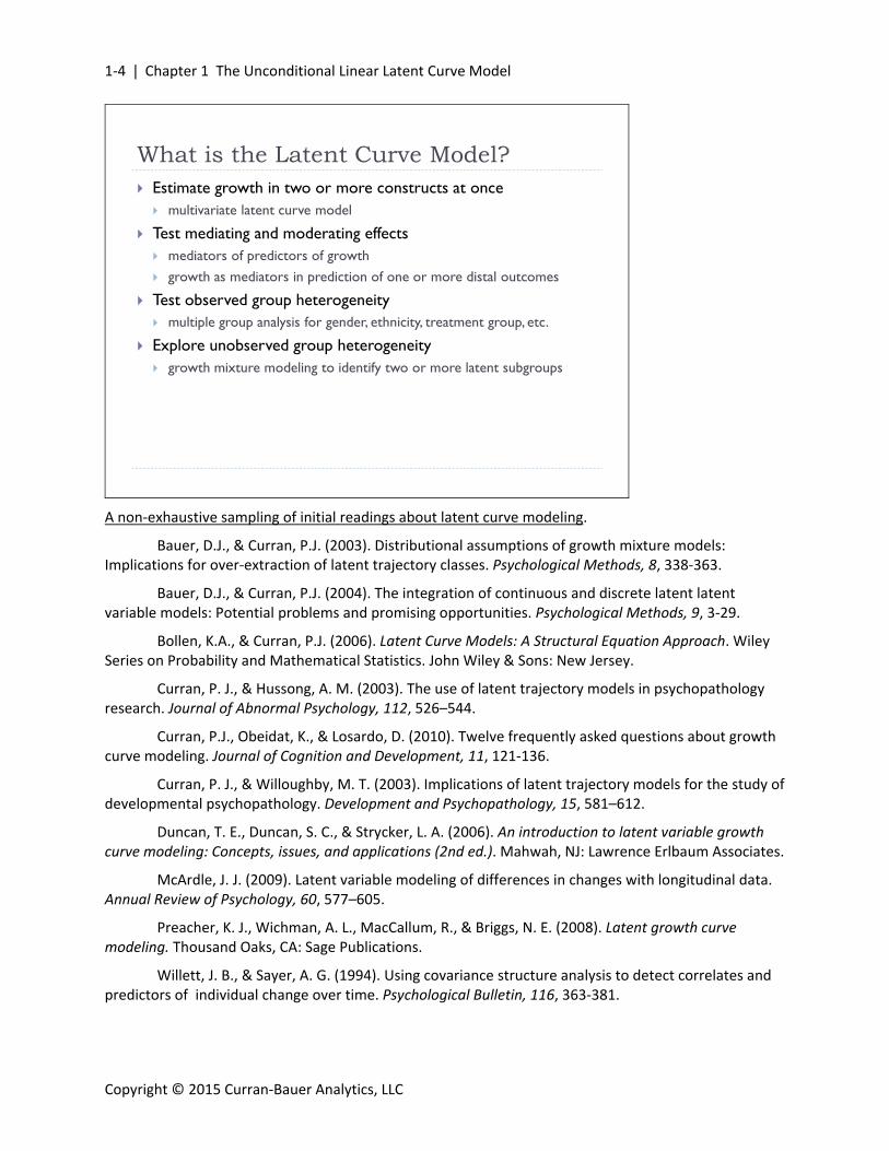
Curran, Bauer & Willoughby (2004)

Curran, P.J., Bauer, D.J., & Willoughby, M.T. (2004). Testing main effects and interactions in latent curve analysis. Psychological Methods, 9, 220‐237.

Abstract from manuscript: A key strength of latent curve analysis (LCA) is the ability to model individual variability in rates of change as a function of 1 or more explanatory variables. The measurement of time plays a critical role because the explanatory variables multiplicatively interact with time in the prediction of the repeated measures. However, this interaction is not typically capitalized on in LCA because the measure of time is rather subtly incorporated via the factor loading matrix. The authors’ goal is to demonstrate both analytically and empirically that classic techniques for probing interactions in multiple regression can be generalized to LCA. A worked example is presented, and the use of these techniques is recommended whenever estimating conditional LCAs in practice.



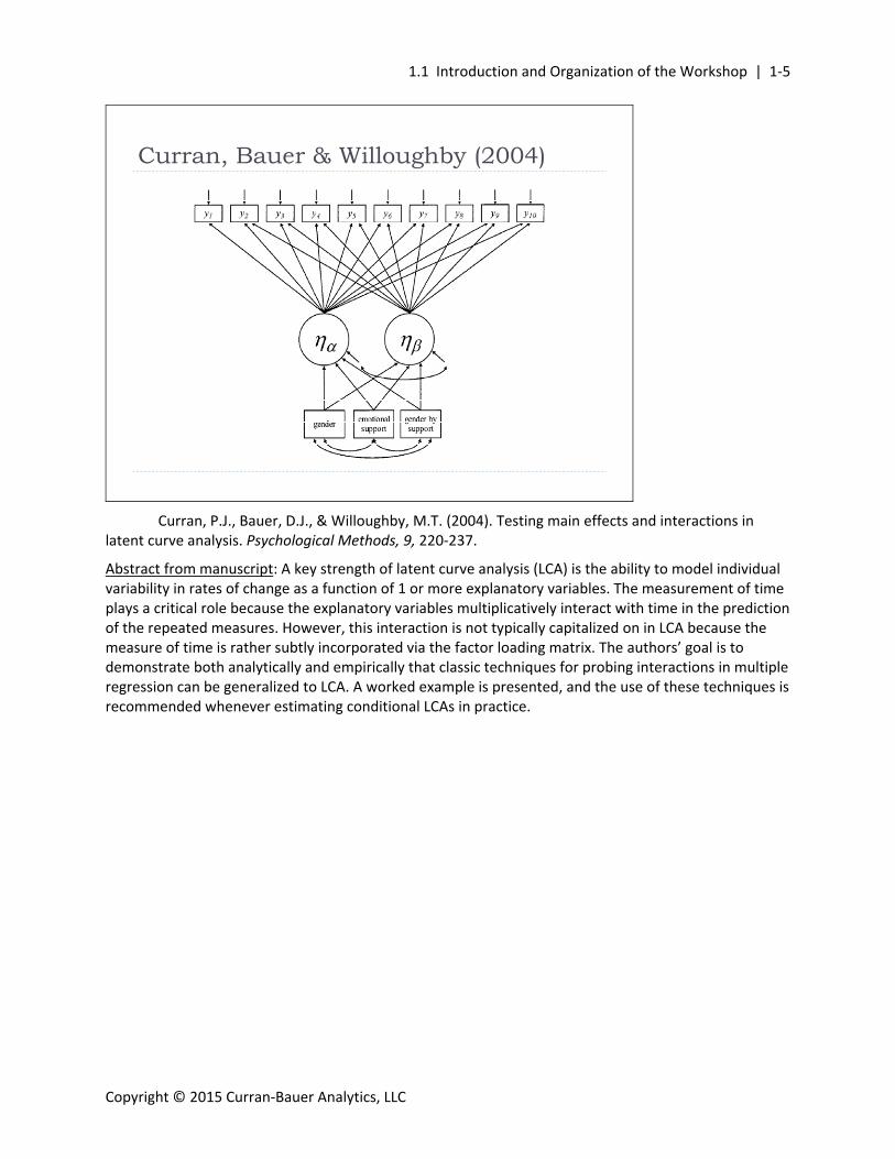
Cole et al. (2002)

Cole. D.A., Tram, J.M., Martin, J.M., Hoffman, K.B., Ruiz, M.D., Jacquez, F.M., & Maschman, T.L. (2002). Individual differences in the emergence of depressive symptoms in children and adolescents: A longitudinal investigation of parent and child reports. Journal of Abnormal Psychology, 111, 156‐165.

Abstract from manuscript: The authors address questions about the rate that depressive symptoms emerge, developmental and gender differences in this rate, and differences between parent and child estimates of this rate. In a 12‐wave, cohort‐sequential, longitudinal design, 1,570 children (Grades 4–11) and parents completed reports about children’s depression. Cross‐domain latent growth curve analysis revealed that (a) the rate of symptom growth varied with developmental level, (b) gender differences symptom growth preceded emergence of mean level gender differences, (c) the rate of symptom development varied with age, and (d) parent– child agreement about rate of symptom change was stronger than agreement about time‐specific symptoms. The authors suggest that predictability of depressive symptoms varies with age and the dimension under investigation.



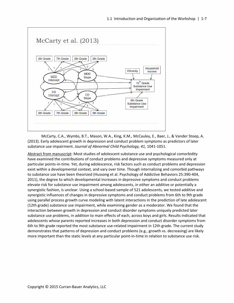
McCarty et al. (2013)

McCarty, C.A., Wymbs, B.T., Mason, W.A., King, K.M., McCauley, E., Baer, J., & Vander Stoep, A. (2013). Early adolescent growth in depression and conduct problem symptoms as predictors of later substance use impairment. Journal of Abnormal Child Psychology, 41, 1041‐1051.

Abstract from manuscript: Most studies of adolescent substance use and psychological comorbidity have examined the contributions of conduct problems and depressive symptoms measured only at particular points‐in‐time. Yet, during adolescence, risk factors such as conduct problems and depression exist within a developmental context, and vary over time. Though internalizing and comorbid pathways to substance use have been theorized (Hussong et al. Psychology of Addictive Behaviors 25:390‐404, 2011), the degree to which developmental increases in depressive symptoms and conduct problems elevate risk for substance use impairment among adolescents, in either an additive or potentially a synergistic fashion, is unclear. Using a school‐based sample of 521 adolescents, we tested additive and synergistic influences of changes in depressive symptoms and conduct problems from 6th to 9th grade using parallel process growth curve modeling with latent interactions in the prediction of late adolescent (12th grade) substance use impairment, while examining gender as a moderator. We found that the interaction between growth in depression and conduct disorder symptoms uniquely predicted later substance use problems, in addition to main effects of each, across boys and girls. Results indicated that adolescents whose parents reported increases in both depression and conduct disorder symptoms from 6th to 9th grade reported the most substance use‐related impairment in 12th grade. The current study demonstrates that patterns of depression and conduct problems (e.g., growth vs. decreasing) are likely more important than the static levels at any particular point‐in‐time in relation to substance use risk.



Structure of the Next Three Days Introduce concept of a latent growth curve

Define latent curve as a confirmatory factor analysis model

Discuss estimation of linear and nonlinear forms of growth

Test and plot effects of time-invariant & time-varying predictors

Build LCMs for two constructs at once

Fit LCMs to non-normal or discrete RMs (skewed, binary, ordinal)

Estimate LCM as a function of two or more observed groups

Estimate LCM as a function of two or more latent groups

Intersperse lecture with software demonstrations in Mplus

Assume prior exposure to SEM, but see Appendix A for a review

Although we focus exclusively on Mplus for our demonstrations, the vast majority of latent curve models can be equivalently estimated using any standard software package including Amos, CALIS, EQS, R (lavaan), LISREL, OpenMx, or Stata (sem).

1.2 Defining a Latent Growth Curve | 1‐9


1.2 DefiningaLatentGrowthCurve

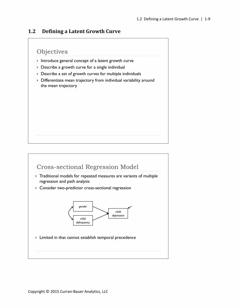
Objectives Introduce general concept of a latent growth curve

Describe a growth curve for a single individual

Describe a set of growth curves for multiple individuals

Differentiate mean trajectory from individual variability around the mean trajectory

Traditional models for repeated measures are variants of multiple regression and path analysis

Consider two-predictor cross-sectional regression

Limited in that cannot establish temporal precedence

Cross-sectional Regression Model

childdepression

gender

childdelinquency



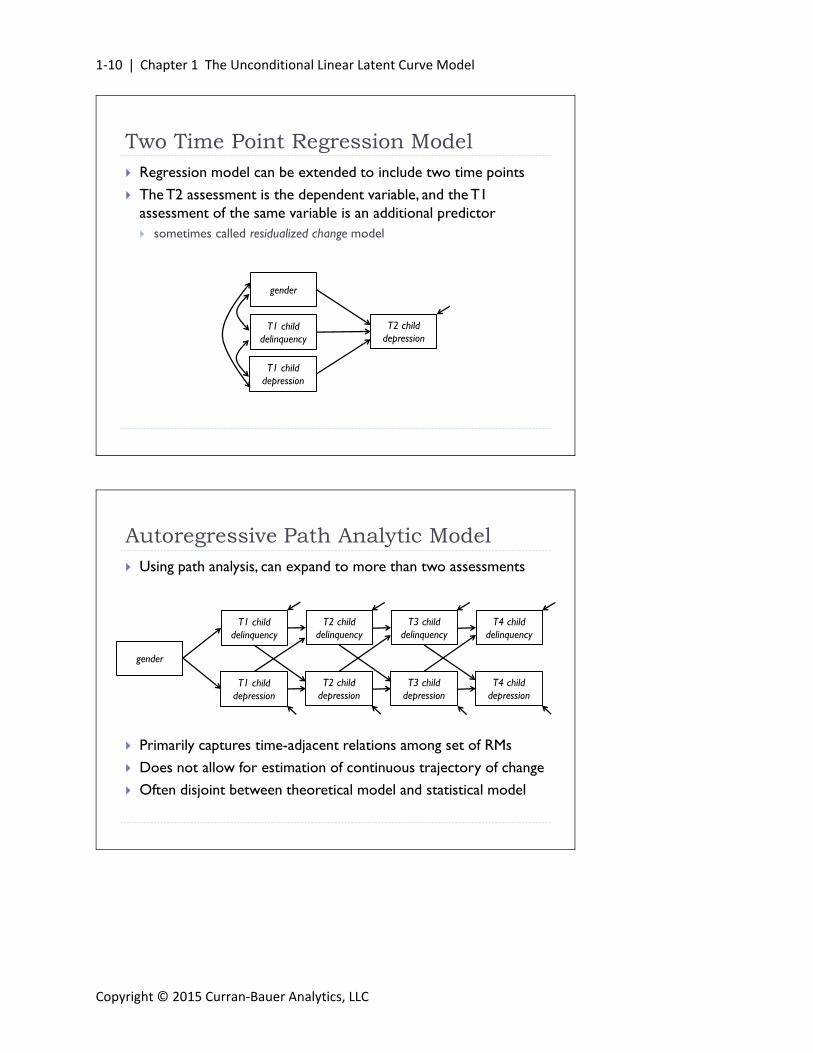
Regression model can be extended to include two time points

The T2 assessment is the dependent variable, and the T1 assessment of the same variable is an additional predictor sometimes called residualized change model

Two Time Point Regression Model

T2 childdepression

gender

T1 childdelinquency

T1 childdepression

Autoregressive Path Analytic Model Using path analysis, can expand to more than two assessments

Primarily captures time-adjacent relations among set of RMs

Does not allow for estimation of continuous trajectory of change

Often disjoint between theoretical model and statistical model

T2 childdelinquency

T4 childdelinquency

T3 childdelinquency

gender

T1 childdelinquency

T2 childdepression

T4 childdepression

T3 childdepression

T1 childdepression



The Latent Growth Curve To capture continuous trajectory of change, will approach

precisely same data structure from different perspective

Will build model for data that estimates change over time withineach individual and then compare change across individuals e.g., estimate inter-individual variability in intra-individual change

This is core concept behind a growth curve also sometimes called latent trajectories, latent curves, growth

trajectories, or time paths

Although growth models are often described as first fitting trajectories to each individual observation and then examining the set of trajectories across all individuals, the models are typically estimated in a single analytic step.

Repeated Measures for One Person Consider hypothetical case where we have five repeated

measures assessing depression in a single adolescent

time

de

pre

ssio

n



Could connect observations to see time-adjacent changes

Repeated Measures for One Person

time

de

pre

ssio

n

A Growth Curve for One Person Could instead “smooth over” repeated measures and estimate a

line of best fit for this individual

time

de

pre

ssio

n



Can summarize line by two pieces of information the intercept ( ) and the slope ( ) unique to individual i

A Growth Curve for One Person

time

de

pre

ssio

n

1i

2i

We use the 1i and 2 i to denote intercept and slope so that later latent curve models correspond with

the standard notation used in the general SEM.

Growth Curves for Multiple Persons Rarely interested in one individual, but in a sample of individuals

can extend to 8 trajectories (but would use 100 or more in practice)

can also consider the mean and variance of the 8 trajectories

de

pre

ssio

n

time

individual trajectories

mean trajectory



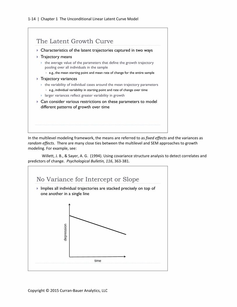
Characteristics of the latent trajectories captured in two ways

Trajectory means the average value of the parameters that define the growth trajectory

pooling over all individuals in the sample e.g., the mean starting point and mean rate of change for the entire sample

Trajectory variances the variability of individual cases around the mean trajectory parameters

e.g., individual variability in starting point and rate of change over time

larger variances reflect greater variability in growth

Can consider various restrictions on these parameters to model different patterns of growth over time

The Latent Growth Curve

In the multilevel modeling framework, the means are referred to as fixed effects and the variances as random effects. There are many close ties between the multilevel and SEM approaches to growth modeling. For example, see:

Willett, J. B., & Sayer, A. G. (1994). Using covariance structure analysis to detect correlates and predictors of change. Psychological Bulletin, 116, 363‐381.

No Variance for Intercept or Slope Implies all individual trajectories are stacked precisely on top of

one another in a single line

de

pre

ssio

n

time



Mean Slope, Mean & Variance Intercept Implies individual variability in starting point but constant rate of

change over time

de

pre

ssio

n

time

Mean & Variance both Intercept & Slope Implies individual variability in starting point and rate of change

de

pre

ssio

n

time



Initial Motivating Questions What is the mean course of change over time?

linear, quadratic, exponential, no change, etc.

Are there individual differences in the course of change? variability in starting point and rate of change

Are there time-invariant predictors of change? person-level characteristics like gender, ethnicity diagnostic status

Are there time-varying predictors of change? time-specific characteristics like onset of drinking, arrest, marriage

Do two constructs travel together through time? trajectories of alcohol use linked with trajectories of depression

Do trajectories meaningfully vary as function of observed or latent group membership?

Summary Initial motivation is that there exists a true underlying continuous

trajectory of change that was not directly observed

Want to use the observed repeated measures to infer existence of underlying latent trajectory

Means capture overall values of parameters that define growth trajectory

Variances capture individual variability in parameters that define growth trajectory

Goal is to build a model that incorporates predictors of individual variability in growth

Will build this model using the SEM analytical framework

1.3 Latent Growth Curves as a Confirmatory Factor Model | 1‐17


1.3 LatentGrowthCurvesasaConfirmatoryFactorModel

Objectives Briefly review confirmatory factor analysis (CFA) model

Define latent curve as a special type of CFA

Explore mean and covariance structures implied by the LCM

Capturing Growth as a Latent Factor Theory posits existence of unobserved continuous trajectory

Cannot directly observe, but can infer existence based on set of repeated measures

Growth curve thus fits naturally into latent variable model e.g., depression, self esteem, worker productivity, etc.

Can draw on strengths of confirmatory factor analysis (CFA) to define latent curve model

The LCM is fundamentally a highly restricted CFA model it is thus helpful to first review the standard CFA so we may then modify

this to define the LCM



Confirmatory Factor Analysis Primarily theory-driven: test model that specifies the number and

nature of the latent factors behind set of observed measures e.g., latent depression and anxiety underlie set of 20 symptom items

Model identified through restrictions on parameters

Number of latent factors determined by theory

Factor pattern matrix is restricted by analyst to reflect theory e.g., some loadings freely estimated, others fixed to zero

Attention paid to global and local fit of model to data

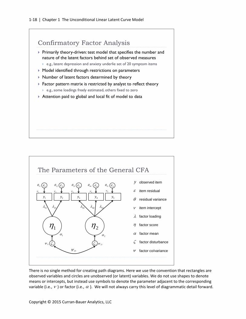
The Parameters of the General CFA

item residual

item intercept

factor loading

factor score

factor mean

factor disturbance

y observed item

1

11 21 32 42

1 2 3 4

1 2 3 4

1

1

1y 2y 3y 4y

2

2

5

5

5y

52

2

21 factor co/variance

1122

11 22 33 44 55

residual variance

There is no single method for creating path diagrams. Here we use the convention that rectangles are observed variables and circles are unobserved (or latent) variables. We do not use shapes to denote means or intercepts, but instead use symbols to denote the parameter adjacent to the corresponding variable (i.e., ) or factor (i.e., ). We will not always carry this level of diagrammatic detail forward.



The Measurement Equation Measurement equation expresses observed vector of measures

as function of underlying latent factors

There are p-observed variables and k-latent factors

i i i y ν Λη ε

1 11 11 1 1

2 2 21 2 22

1

i ik i

i k ii

p kpppi piki

y

y

y

See Appendix A for a review of the general structural equation model.

The Measurement Equation Further, the residuals from the measurement equation

are distributed as

where

i i i y ν Λη ε

11

220

0 0

0 0 0 pp

Θ

~ ,i MVNε 0 Θ



The Structural Equation Next define model for latent factors in the structural equation

for k-latent factors

i i η α ζ

1 11

2 2 2

i i

i i

kki ki

The Structural Equation The deviations from the structural model

are distributed as

where

i i η α ζ

11

21 22

1 2k k kk

Ψ

~ ,i MVNζ 0 Ψ



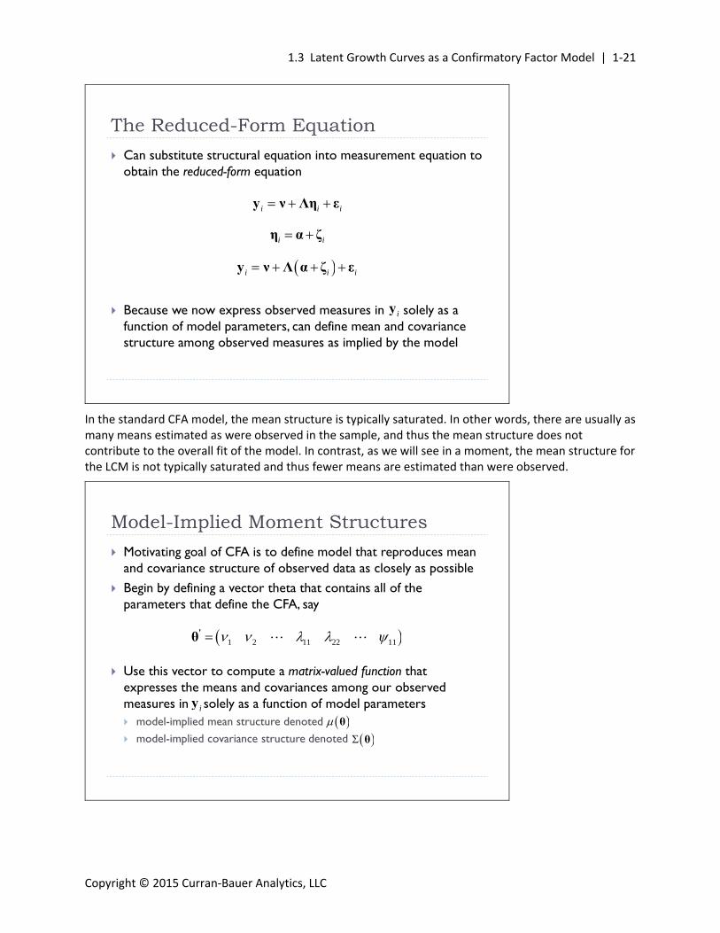
Can substitute structural equation into measurement equation to obtain the reduced-form equation

Because we now express observed measures in solely as a function of model parameters, can define mean and covariance structure among observed measures as implied by the model

The Reduced-Form Equation

i i i y ν Λ α ζ ε

i i η α ζ

i i i y ν Λη ε

iy

In the standard CFA model, the mean structure is typically saturated. In other words, there are usually as many means estimated as were observed in the sample, and thus the mean structure does not contribute to the overall fit of the model. In contrast, as we will see in a moment, the mean structure for the LCM is not typically saturated and thus fewer means are estimated than were observed.

Motivating goal of CFA is to define model that reproduces mean and covariance structure of observed data as closely as possible

Begin by defining a vector theta that contains all of the parameters that define the CFA, say

Use this vector to compute a matrix-valued function that expresses the means and covariances among our observed measures in solely as a function of model parameters model-implied mean structure denoted

model-implied covariance structure denoted

Model-Implied Moment Structures

1 2 11 22 11 'θ

θ

θ

iy



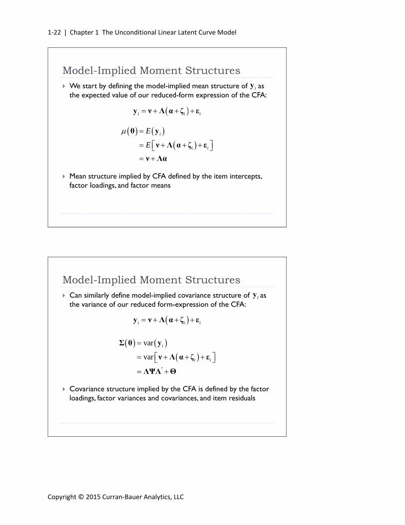
We start by defining the model-implied mean structure of as the expected value of our reduced-form expression of the CFA:

Mean structure implied by CFA defined by the item intercepts, factor loadings, and factor means

i

i i

E

E

θ y

ν Λ α ζ ε

ν Λα


iy


Can similarly define model-implied covariance structure of as the variance of our reduced form-expression of the CFA:

Covariance structure implied by the CFA is defined by the factor loadings, factor variances and covariances, and item residuals


iy


var

var

i

i i

'

Σ θ y

ν Λ α ζ ε

ΛΨΛ Θ



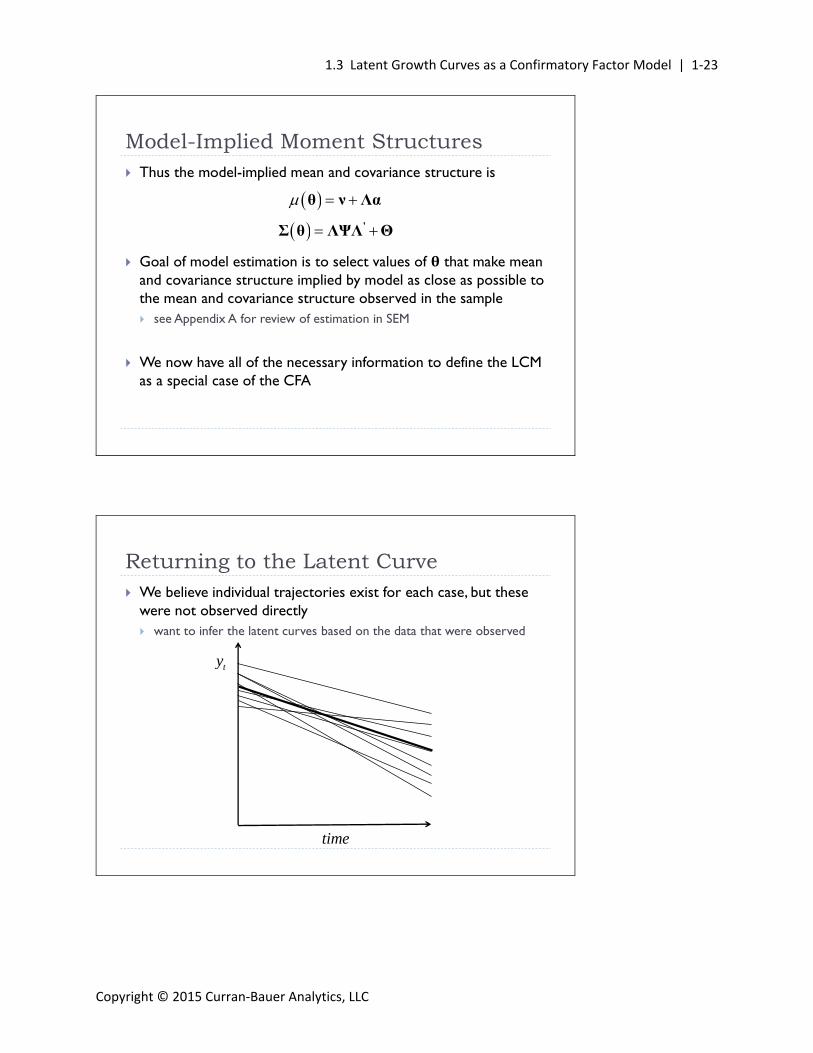
Thus the model-implied mean and covariance structure is

Goal of model estimation is to select values of that make mean and covariance structure implied by model as close as possible to the mean and covariance structure observed in the sample see Appendix A for review of estimation in SEM

We now have all of the necessary information to define the LCM as a special case of the CFA

θ ν Λα


'Σ θ ΛΨΛ Θ

Returning to the Latent Curve We believe individual trajectories exist for each case, but these

were not observed directly want to infer the latent curves based on the data that were observed

time

ty



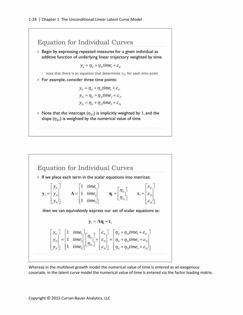
Equation for Individual Curves Begin by expressing repeated measures for a given individual as

additive function of underlying linear trajectory weighted by time

note that there is an equation that determines for each time point

For example, consider three time points:

Note that the intercept ( ) is implicitly weighted by 1, and the slope ( ) is weighted by the numerical value of time

1 2ti i i t tiy time

1 1 2 1 1

2 1 2 2 2

3 1 2 3 3

i i i i

i i i i

i i i i

y time

y time

y time

Equation for Individual Curves If we place each term in the scalar equations into matrices:

then we can equivalently express our set of scalar equations as:

1

2

3

1

1

1

time

time

time

Λ 1

2

ii

i

η1

2

3

i

i i

i

ε1

2

3

i

i i

i

y

y

y

y

1 1 1 2 1 111

2 2 2 1 2 2 22

33 3 1 2 3 3

1

1

1

i i i i ii

i i i i ii

i i i i i

y timetime

y time time

timey time

i i i y Λη ε

Whereas in the multilevel growth model the numerical value of time is entered as an exogenous covariate, in the latent curve model the numerical value of time is entered via the factor loading matrix.



The Measurement Equation Note similarity of LCM equation:

to CFA equation from earlier:

Indeed, measurement equation for the LCM is the same as the measurement equation for the CFA with the restriction that

item-specific intercepts are restricted to zero and LCM must reproduce sample means entirely through means of latent factor

We next need to define a model for the latent curve factors

i i i y ν Λη ε

ν 0

i i i y Λη ε

The triple equal sign (i.e., ) means "is equal to by definition", so 0ν indicates that the vector of item intercepts are fixed to zero.

The Structural Equation Recall we can write the intercept and slope as a function of the

mean and individual deviation from the mean:

We can again compactly summarize these in matrix form

This expression precisely matches that of the CFA

1 11 11

2 22 2 2

ii i

i i i

i i η α ζ

1 1 1

2 2 2

i i

i i



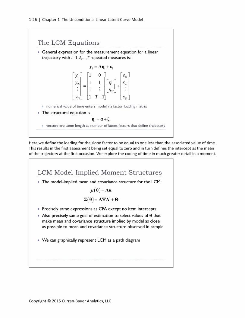
The LCM Equations General expression for the measurement equation for a linear

trajectory with t=1,2,...,T repeated measures is:

numerical value of time enters model via factor loading matrix

The structural equation is

vectors are same length as number of latent factors that define trajectory

1 1

2 1 2

2

1 0

1 1

1 1

i i

i i i

i

Ti Ti

y

y

y T

i i i y Λη ε

i i η α ζ

Here we define the loading for the slope factor to be equal to one less than the associated value of time. This results in the first assessment being set equal to zero and in turn defines the intercept as the mean of the trajectory at the first occasion. We explore the coding of time in much greater detail in a moment.

The model-implied mean and covariance structure for the LCM:

Precisely same expressions as CFA except no item intercepts

Also precisely same goal of estimation to select values of that make mean and covariance structure implied by model as close as possible to mean and covariance structure observed in sample

We can graphically represent LCM as a path diagram

θ Λα

LCM Model-Implied Moment Structures

'Σ θ ΛΨΛ Θ



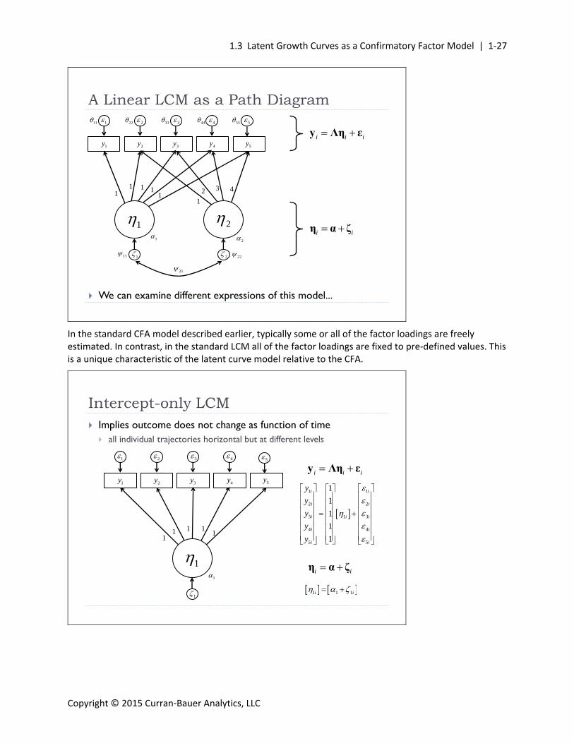
We can examine different expressions of this model...

A Linear LCM as a Path Diagram

i i i y Λη ε

i i η α ζ

1

1 2 3 4

1

1

1y 2y 3y 4y

5

5y

1 1 11

1

2 3 4

1 2

2

2

21

1122

11 22 33 44 55

In the standard CFA model described earlier, typically some or all of the factor loadings are freely estimated. In contrast, in the standard LCM all of the factor loadings are fixed to pre‐defined values. This is a unique characteristic of the latent curve model relative to the CFA.

Implies outcome does not change as function of time all individual trajectories horizontal but at different levels

Intercept-only LCM

1 1

2 2

3 31

4 4

5 5

1

1

1

1

1

i i

i i

i ii

i i

i i

y

y

y

y

y

1 1 1i i

i i η α ζ

i i i y Λη ε

1

1 2 3 4

1

1

1y 2y 3y 4y

5

5y

1 1 11

1



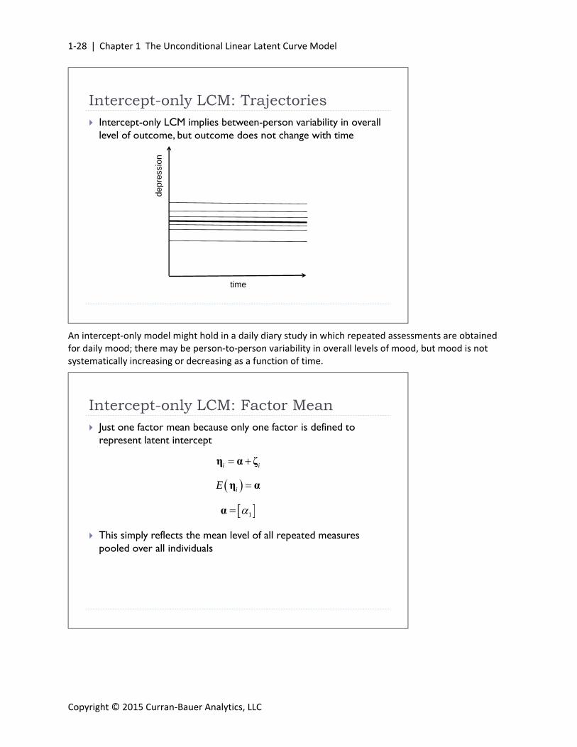
Intercept-only LCM: Trajectories Intercept-only LCM implies between-person variability in overall

level of outcome, but outcome does not change with time

time

de

pre

ssio

n

An intercept‐only model might hold in a daily diary study in which repeated assessments are obtained for daily mood; there may be person‐to‐person variability in overall levels of mood, but mood is not systematically increasing or decreasing as a function of time.

Just one factor mean because only one factor is defined to represent latent intercept

This simply reflects the mean level of all repeated measures pooled over all individuals

iE η α

i i η α ζ

1α

Intercept-only LCM: Factor Mean



Just one factor variance again because only one factor is defined to represent latent intercept

This represents the individual variability around the overall mean

~ ,i Nζ 0 Ψ

11Ψ

i i η α ζ

Intercept-only LCM: Factor Variance

Finally, time-specific residuals for RMs allowed to obtain a unique value at each time point and are typically uncorrelated over time

~ ,i Nε 0 Θ

11

22

33

44

55

0

0 0

0 0 0

0 0 0 0

Θ

i i i y Λη ε

Intercept-only LCM: Residual Variance

Here we estimate a unique residual variance at each time period; this is called heteroscedasticity. In a moment we will compare this to a model in which we estimate a single residual variance for all time periods; this is called homoscedasticity.



Linear LCM Can add a second correlated factor to capture linear change:

i i i y Λη ε

1 1

2 21

3 32

4 4

5 5

1 0

1 1

1 2

1 3

1 4

i i

i ii

i ii

i i

i i

y

y

y

y

y

i i η α ζ

1 11

2 2 2

ii

i i

1

1 2 3 4

1

1

1y 2y 3y 4y

5

5y

1 1 11

1

2 3 4

1 2

2

2

21

1122

11 22 33 44 55

In this chapter we focus explicitly on the linear growth model. We will expand this to a variety of nonlinear functions in Chapter 2.

Linear LCM: Trajectories Intercept and linear slope model implies individual differences in

both level and rate of change

de

pre

ssio

n

time



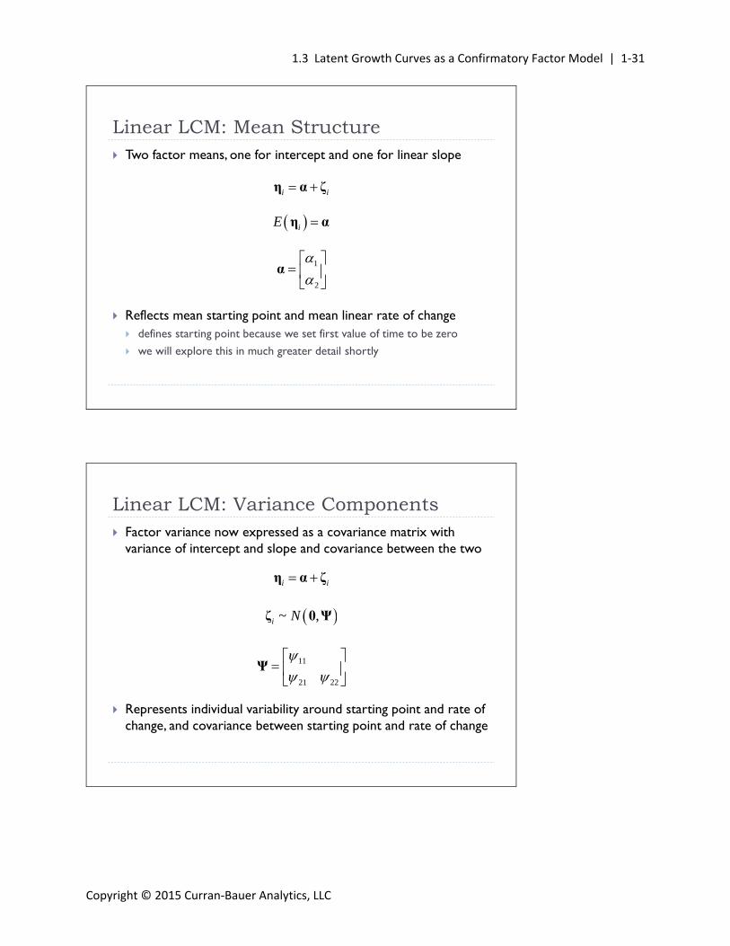
Two factor means, one for intercept and one for linear slope

Reflects mean starting point and mean linear rate of change defines starting point because we set first value of time to be zero

we will explore this in much greater detail shortly

iE η α

i i η α ζ

1

2

α

Linear LCM: Mean Structure

Factor variance now expressed as a covariance matrix with variance of intercept and slope and covariance between the two

Represents individual variability around starting point and rate of change, and covariance between starting point and rate of change

~ ,i Nζ 0 Ψ

11

21 22

Ψ

i i η α ζ

Linear LCM: Variance Components



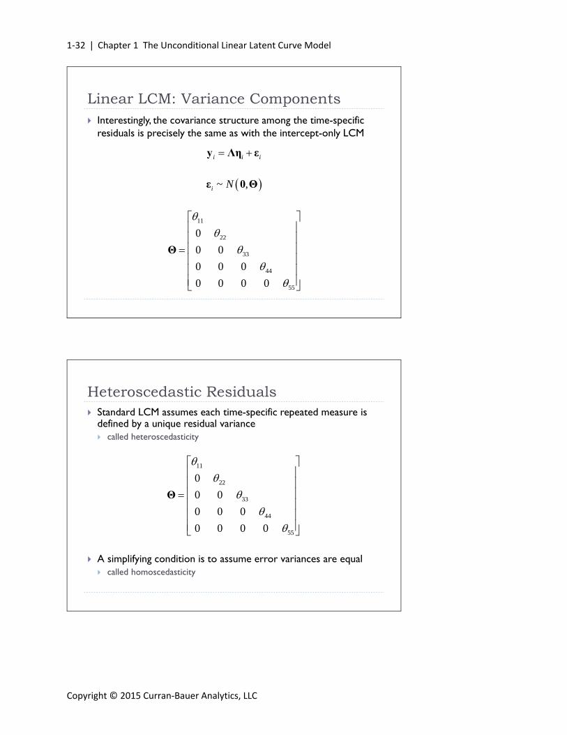
Interestingly, the covariance structure among the time-specific residuals is precisely the same as with the intercept-only LCM

~ ,i Nε 0 Θ

11

22

33

44

55

0

0 0

0 0 0

0 0 0 0

Θ

i i i y Λη ε

Linear LCM: Variance Components

Heteroscedastic Residuals Standard LCM assumes each time-specific repeated measure is

defined by a unique residual variance called heteroscedasticity

A simplifying condition is to assume error variances are equal called homoscedasticity

11

22

33

44

55

0

0 0

0 0 0

0 0 0 0

Θ



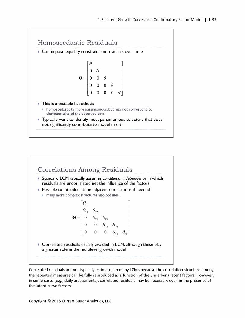
Homoscedastic Residuals Can impose equality constraint on residuals over time

This is a testable hypothesis homoscedasticity more parsimonious, but may not correspond to

characteristics of the observed data

Typically want to identify most parsimonious structure that does not significantly contribute to model misfit

0

0 0

0 0 0

0 0 0 0

Θ

Correlations Among Residuals Standard LCM typically assumes conditional independence in which

residuals are uncorrelated net the influence of the factors Possible to introduce time-adjacent correlations if needed

many more complex structures also possible

Correlated residuals usually avoided in LCM, although these play a greater role in the multilevel growth model

11

21 22

32 33

43 44

54 55

0

0 0

0 0 0

Θ

Correlated residuals are not typically estimated in many LCMs because the correlation structure among the repeated measures can be fully reproduced as a function of the underlying latent factors. However, in some cases (e.g., daily assessments), correlated residuals may be necessary even in the presence of the latent curve factors.



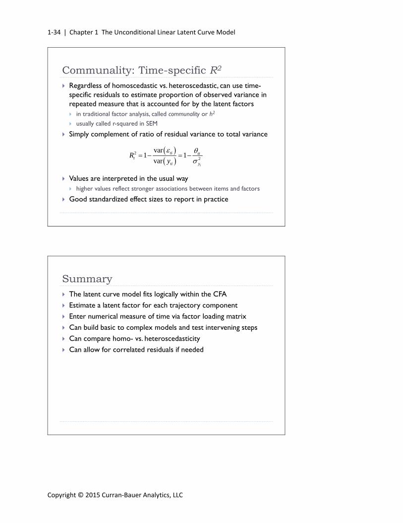
Communality: Time-specific R2

Regardless of homoscedastic vs. heteroscedastic, can use time-specific residuals to estimate proportion of observed variance in repeated measure that is accounted for by the latent factors in traditional factor analysis, called communality or h2

usually called r-squared in SEM

Simply complement of ratio of residual variance to total variance

Values are interpreted in the usual way higher values reflect stronger associations between items and factors

Good standardized effect sizes to report in practice

22

var1 1

vart

ti ttt

ti y

Ry

Summary The latent curve model fits logically within the CFA

Estimate a latent factor for each trajectory component

Enter numerical measure of time via factor loading matrix

Can build basic to complex models and test intervening steps

Can compare homo- vs. heteroscedasticity

Can allow for correlated residuals if needed

1.4 Thinking More Closely About Time | 1‐35


1.4 ThinkingMoreCloselyAboutTime

Objectives More closely consider role of time in the LCM with regard to

where to place the zero point

the unequal spacing of time

alternative units of time individually-varying assessments of time

Up to this point we have set numerical value of time to equal zero at the first assessment period:

0, 1, 2, 3t

0 1 2 3

Mean and variance of intercept is scaled for initial time period because when time iszero the slope factordoes not contribute

Coding Time: Zero Point

Note that t denotes the numerical scaling of time and appears in the second column of the factor

loading matrix for a linear LCM (where the first column consists of all 1’s to define the intercept factor).



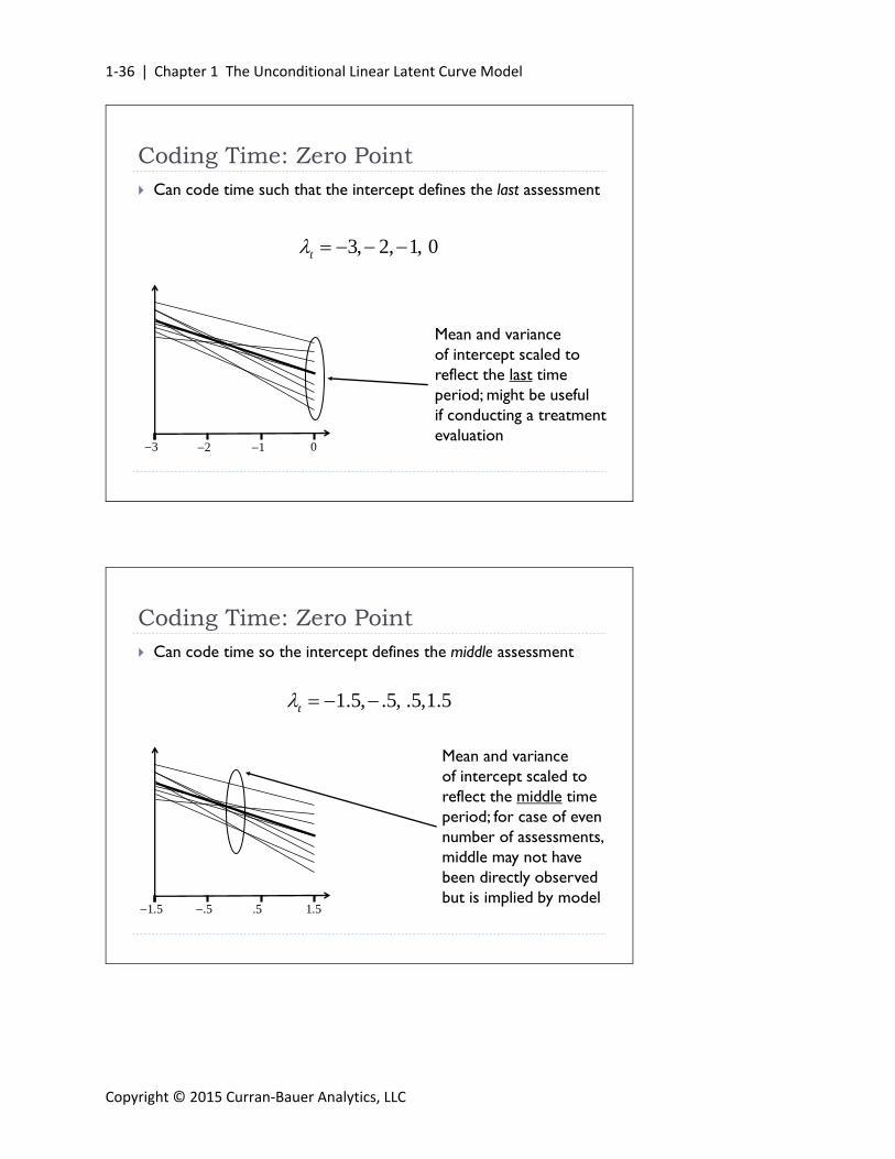
Can code time such that the intercept defines the last assessment

3, 2, 1, 0t

3 2 1 0

Mean and variance of intercept scaled to reflect the last time period; might be usefulif conducting a treatmentevaluation


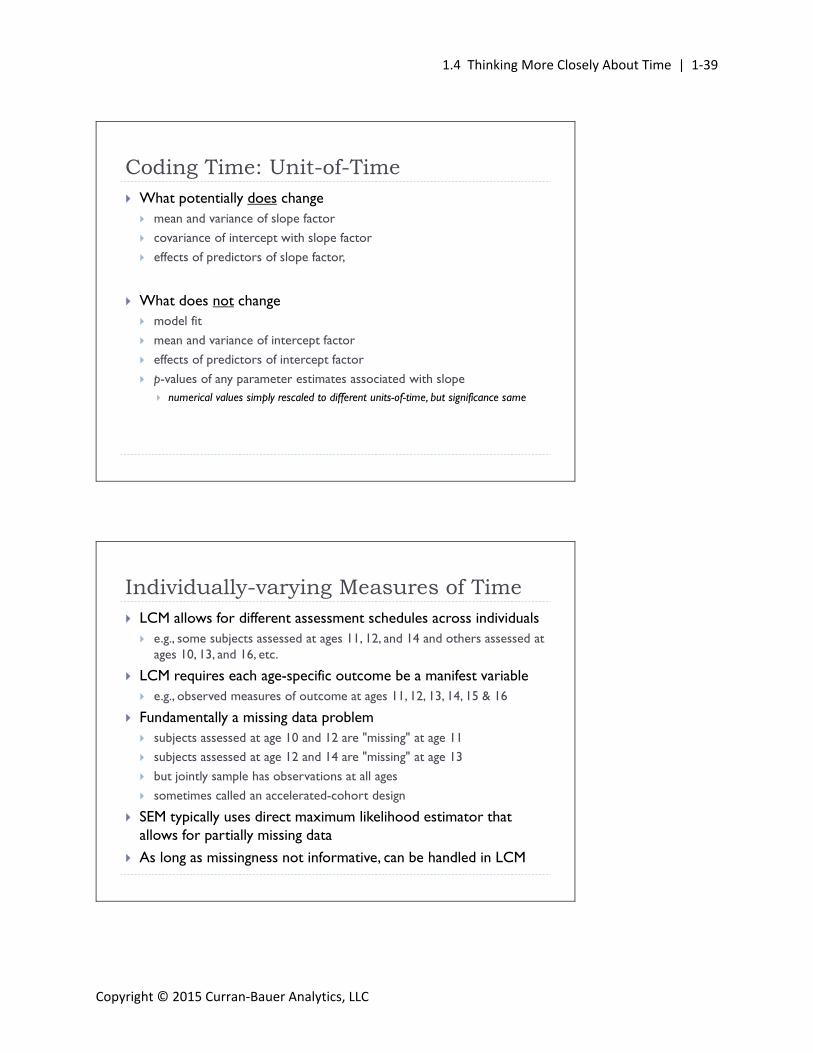
Can code time so the intercept defines the middle assessment

1.5, .5, .5,1.5t

1.5 .5 .5 1.5

Mean and variance of intercept scaled to reflect the middle time period; for case of evennumber of assessments, middle may not have been directly observedbut is implied by model




Alternative coding schemes for time are done via factor loadings

All of these result in same model fit, but several properties of LCM change depending on the numerical coding of time

1 0

1 1

1 2

1 3

1 3

1 2

1 1

1 0

1 1.5

1 0.5

1 0.5

1 1.5


What potentially does change the mean of the intercept factor

the variance of the intercept factor

the covariance between the intercept and slope factor effects of predictors of the intercept factor

What does not change model fit

the mean of the linear slope factor

the variance of the linear slope factor

effects of predictors of the linear slope factor


The above summary holds for the linear LCM. Some complications arise in coding of time when considering higher‐order polynomial functions (e.g., quadratic or cubic). For details, see:

Biesanz, J.C., Deeb‐Sossa, N., Aubrecht, A.M., Bollen, K.A., & Curran, P.J. (2004). The role of coding time in estimating and interpreting growth curve models. Psychological Methods, 9, 30‐52.



Thus far have assumed equally spaced assessments e.g., one year increment between each assessment

No reason to be limited to equally spaced assessment periods can have some or even all assessments unequally spaced

For example, say assessed subjects at ages 6, 7, 10, 12, & 16 factor loadings simply scaled relative to spacing of first two assessments

All of our prior discussion about placement of the zero point holds here as well

Coding Time: Spacing

' 1 1 1 1 1

0 1 4 6 10

Λ

Coding Time: Unit-of-Time We also control the unit of time under study

e.g., assessments taken at 6, 12, 18, 30, and 42 months

Can scale time in months, half-years, or full-years

All models fit identically, but mean and variance of slope factor scaled in the given unit of time

1 0

1 1

1 2

1 4

1 6

half year

Λ

1 0

1 .5

1 1

1 2

1 3

full year

Λ

1 0

1 6

1 12

1 24

1 36

month

Λ

Both the choice of zero‐point, spacing, and unit of time can be controlled with a single linear transformation equation; see Bollen & Curran (2006), pages 115‐120.

Bollen, K.A., & Curran, P.J. (2006). Latent Curve Models: A Structural Equation Approach. Wiley Series on Probability and Mathematical Statistics. John Wiley & Sons: New Jersey.



Coding Time: Unit-of-Time What potentially does change

mean and variance of slope factor

covariance of intercept with slope factor

effects of predictors of slope factor,

What does not change model fit

mean and variance of intercept factor

effects of predictors of intercept factor

p-values of any parameter estimates associated with slope numerical values simply rescaled to different units-of-time, but significance same

Individually-varying Measures of Time LCM allows for different assessment schedules across individuals

e.g., some subjects assessed at ages 11, 12, and 14 and others assessed at ages 10, 13, and 16, etc.

LCM requires each age-specific outcome be a manifest variable e.g., observed measures of outcome at ages 11, 12, 13, 14, 15 & 16

Fundamentally a missing data problem subjects assessed at age 10 and 12 are "missing" at age 11 subjects assessed at age 12 and 14 are "missing" at age 13

but jointly sample has observations at all ages

sometimes called an accelerated-cohort design

SEM typically uses direct maximum likelihood estimator that allows for partially missing data

As long as missingness not informative, can be handled in LCM



Individually-varying Measures of Time Some longitudinal designs have highly variable assessments

e.g., daily diary data where subjects randomly pinged throughout day

At the extreme, could have no two people provide assessments at same time point

Standard LCM not well suited for data such as these must be able to compute mean and variance of RM at each time period

Must instead use definition variable methodology in LCM defines a unique factor loading matrix for each person based on person-

specific time scores, then fits LCM aggregating over individual matrices

Places the LCM much closer to a multilevel modeling approach indeed, MLM may be a better analytic strategy

Boker, S., Neale, M., Maes, H., Wilde, M., Spiegel, M., Brick, T., ... & Fox, J. (2011). OpenMx: an open source extended structural equation modeling framework. Psychometrika, 76, 306‐317.

Neale, M. C., Aggen, S. H., Maes, H. H., Kubarych, T. S., & Schmitt, J. E. (2006). Methodological issues in the assessment of substance use phenotypes. Addictive Behaviors, 31, 1010‐1034.

Summary Can select numerical values of time to achieve different goals

Can define alternative zero-points for time e.g., beginning, middle, or end of trajectory

Can define unequal assessment intervals e.g., 6 month, 12 month, 24 month

Can alter metric of change e.g., days, weeks, months, etc.

Can incorporate individually-varying measures of time definition variables

All centered around ultimate goal of identifying optimal functional form of change over time

1.5 Demonstration: Linear Trajectories of Negative Affect | 1‐41


1.5 Demonstration:LinearTrajectoriesofNegativeAffect

Objectives Introduce real data set studying trajectories of adolescent

depression and delinquency from ages 11 to 16

Fit series of models to repeated measures of depression to identify optimally fitting LCM

Draw initial conclusions about the developmental course of depression prior to including predictors of level and change

Adolescent & Family Development Project Data for demonstration provided by Dr. Laurie Chassin, Director

of the Adolescent and Family Development Project (AFDP)

Demonstration data drawn from much larger sample & measures

Sample consists of n=452 children assessed 1, 2, or 3 times between ages 11 and 16 54% were children of alcoholics (COAs)

53% were male

Outcomes of interest are IRT-based scores of negative affect (NA) based on parent-reports of 13 binary items e.g., lonely, cries a lot, worries, has to be perfect, feels guilty, etc. full details in Bauer et al., (2013)

Unit of analysis is age-specific continuous measure of NA

Bauer, D.J., Howard, A.L., Baldasaro, R.E., Curran, P.J., Hussong, A.M., Chassin, L., & Zucker, R.A. (2013). A trifactor model for integrating ratings across multiple informants. Psychological Methods, 18, 475‐493.



We use an accelerated longitudinal cohort design such that chronological age is our numerical metric of time

This data structure results in missingness introduced by design "x" denotes data that are present

"•" denotes data that are missing

This design allows for a 6 year age span even though no individual child was assessed more than 3 times

Adolescent & Family Development Project

11 12 13 14 15 16

x x x • • •

• x x x • •

• • x x x •

• • • x x x

See Appendix A for a brief review of missing data estimation in SEMs.

Motivating Questions Is there evidence of individual variability in the overall level

negative affect?

Does the inclusion of a linear slope factor significantly improve model fit?

Is there evidence of individual variability in starting point and rate of change over time?

Does the model support the constraint that the time-specific residuals be homoscedastic?

Does the final model adequately fit the observed data?



AdolescentandFamilyDevelopmentProject

The data for this demonstration were drawn from the Adolescent Family Development Project (AFDP) Directed by Dr. Laurie Chassin from Arizona State University. We are indebted to Dr. Chassin for generously sharing these data with us. Note that these data were provided for strictly pedagogical purposes and should not be used for any other purposes beyond this workshop. These data are stored in the file na_ext.dat .

Briefly, the AFDP is a multi‐year longitudinal study of a large sample of adolescents and their parents. Approximately one‐half of the original 452 families were characterized by at least one parent diagnosed as alcoholic (54%), and the remaining were characterized by neither parent diagnosed as alcoholic (46%). Data collection spanned more than two decades, but here we consider just the first three waves of assessment. Parents and children were first assessed when the child was between 11 and 15 years of age, and were re‐assessed up to two more times at 12‐month intervals. Of the 452 families considered here, 358 (79%) were assessed three times, 87 (19%) twice, and 7 (2%) one time. Two child‐specific predictors are of interest: child of an alcoholic (COA) and gender.

The parent's report of the child's negative affect was obtained at each age of assessment. Item response theory (IRT) scores were estimated for 13 binary symptom items indicating the absence or presence of negative affect symptomatology. Sample items include lonely, cries a lot, worries, has to be perfect, and feels guilty. Finally, parent's report of the child's externalizing behavior were obtained at each age of assessment. Item response theory (IRT) scores were estimated for 20 binary symptom items indicating the absence or presence of externalizing symptomatology. Sample items include swearing, truancy, cruelty, destroys things, fights, etc.

The variables in the data set are:

id Unique numerical identifier for each child ranging from 1 to 452

coa 0=child of a non‐alcoholic, 1=child of an alcoholic

male 0=girl, 1=boy

base_ext Continuous measure of externalizing behavior at baseline, mean centered

na11-na16 Age‐specific IRT score for negative affect

ext11-ext16 Age‐specific IRT score for externalizing symptomatology

In this chapter, we demonstrate how to fit a series of growth models to negative affectivity between ages 11 and 16. In later chapters will will consider the two predictors and externalizing symptomatology.

ExaminingDescriptiveStatistics

The focus of our workshop is on the conceptualization and fitting of latent curve models and not on the general use of Mplus. However, there are a variety of powerful features of Mplus that can help us stay as close to our data as possible. We will demonstrate these features throughout the workshop but refer you to the corpus of Mplus support material available online for details.

As a starting point, we can obtain important initial information about our data prior to fitting the LCMs. For example, consider the following code that is stored in file ch01_na_1.inp:



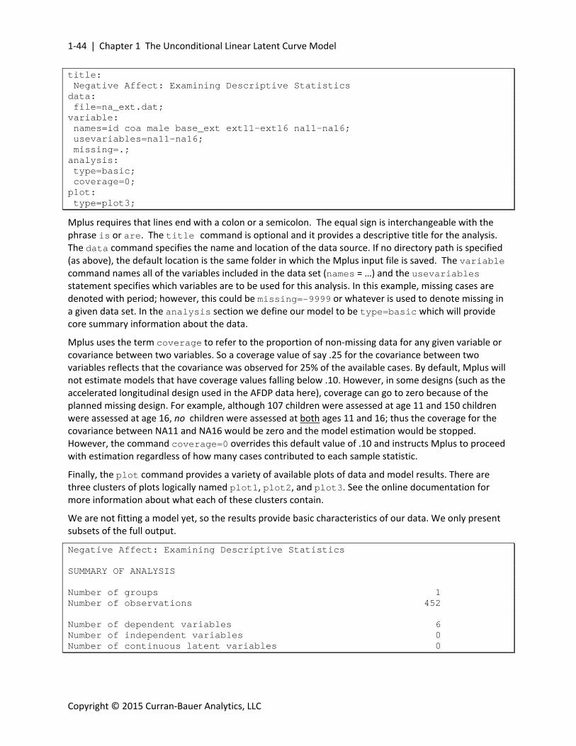
title: Negative Affect: Examining Descriptive Statistics data: file=na_ext.dat; variable: names=id coa male base_ext ext11-ext16 na11-na16; usevariables=na11-na16; missing=.; analysis: type=basic; coverage=0; plot: type=plot3;

Mplus requires that lines end with a colon or a semicolon. The equal sign is interchangeable with the phrase is or are. The title command is optional and it provides a descriptive title for the analysis. The data command specifies the name and location of the data source. If no directory path is specified (as above), the default location is the same folder in which the Mplus input file is saved. The variable command names all of the variables included in the data set (names = …) and the usevariables statement specifies which variables are to be used for this analysis. In this example, missing cases are denoted with period; however, this could be missing=-9999 or whatever is used to denote missing in a given data set. In the analysis section we define our model to be type=basic which will provide core summary information about the data.

Mplus uses the term coverage to refer to the proportion of non‐missing data for any given variable or covariance between two variables. So a coverage value of say .25 for the covariance between two variables reflects that the covariance was observed for 25% of the available cases. By default, Mplus will not estimate models that have coverage values falling below .10. However, in some designs (such as the accelerated longitudinal design used in the AFDP data here), coverage can go to zero because of the planned missing design. For example, although 107 children were assessed at age 11 and 150 children were assessed at age 16, no children were assessed at both ages 11 and 16; thus the coverage for the covariance between NA11 and NA16 would be zero and the model estimation would be stopped. However, the command coverage=0 overrides this default value of .10 and instructs Mplus to proceed with estimation regardless of how many cases contributed to each sample statistic.

Finally, the plot command provides a variety of available plots of data and model results. There are three clusters of plots logically named plot1, plot2, and plot3. See the online documentation for more information about what each of these clusters contain.

We are not fitting a model yet, so the results provide basic characteristics of our data. We only present subsets of the full output.

Negative Affect: Examining Descriptive Statistics SUMMARY OF ANALYSIS Number of groups 1 Number of observations 452 Number of dependent variables 6 Number of independent variables 0 Number of continuous latent variables 0



This indicates that we are considering a single group with 452 individuals and six variables. A variety of useful information is provided about missing data:

SUMMARY OF MISSING DATA PATTERNS MISSING DATA PATTERNS (x = not missing) 1 2 3 4 5 6 7 8 9 10 11 12 13 14 15 16 17 18 19 20 NA11 x x x x x x NA12 x x x x x x x x NA13 x x x x x x x x x x x NA14 x x x x x x x x x x x x x NA15 x x x x x x x NA16 x x x x x x 21 NA11 NA12 NA13 NA14 NA15 NA16 x MISSING DATA PATTERN FREQUENCIES Pattern Frequency Pattern Frequency Pattern Frequency 1 0 8 2 15 2 2 73 9 1 16 94 3 3 10 1 17 4 4 29 11 101 18 3 5 1 12 2 19 1 6 1 13 1 20 46 7 82 14 1 21 4 COVARIANCE COVERAGE OF DATA Minimum covariance coverage value 0.000 PROPORTION OF DATA PRESENT Covariance Coverage NA11 NA12 NA13 NA14 NA15 ________ ________ ________ ________ ________ NA11 0.237 NA12 0.232 0.423 NA13 0.166 0.347 0.588 NA14 0.009 0.192 0.414 0.650 NA15 0.000 0.002 0.226 0.442 0.546 NA16 0.000 0.000 0.007 0.219 0.312 Covariance Coverage NA16 ________ NA16 0.332

This is valuable information about the presence and absence of data across all of the measures. For example, there are no cases for pattern 1 (denoting complete data across all six measures); this reflects



the accelerated cohort sequential design in which no given subject was assessed more than three times, yet we have data spanning six years of age. The highest frequency is pattern 11 at which children were assessed at ages 13, 14 and 15; this too reflects the sample design in which the majority of cases reside at the center of the age span.

The covariance coverage matrix also reflects the design in which no cell exceeds .65 and some cells have zero observed cases (e.g., covariance of ages 11 and 15, 11 and 16, and 12 and 16).

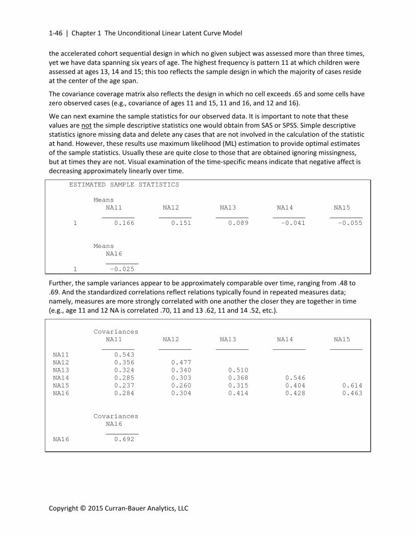
We can next examine the sample statistics for our observed data. It is important to note that these values are not the simple descriptive statistics one would obtain from SAS or SPSS. Simple descriptive statistics ignore missing data and delete any cases that are not involved in the calculation of the statistic at hand. However, these results use maximum likelihood (ML) estimation to provide optimal estimates of the sample statistics. Usually these are quite close to those that are obtained ignoring missingness, but at times they are not. Visual examination of the time‐specific means indicate that negative affect is decreasing approximately linearly over time.

ESTIMATED SAMPLE STATISTICS Means NA11 NA12 NA13 NA14 NA15 ________ ________ ________ ________ ________ 1 0.166 0.151 0.089 -0.041 -0.055 Means NA16 ________ 1 -0.025

Further, the sample variances appear to be approximately comparable over time, ranging from .48 to .69. And the standardized correlations reflect relations typically found in repeated measures data; namely, measures are more strongly correlated with one another the closer they are together in time (e.g., age 11 and 12 NA is correlated .70, 11 and 13 .62, 11 and 14 .52, etc.).

Covariances NA11 NA12 NA13 NA14 NA15 ________ ________ ________ ________ ________ NA11 0.543 NA12 0.356 0.477 NA13 0.324 0.340 0.510 NA14 0.285 0.303 0.368 0.546 NA15 0.237 0.260 0.315 0.404 0.614 NA16 0.284 0.304 0.414 0.428 0.463 Covariances NA16 ________ NA16 0.692



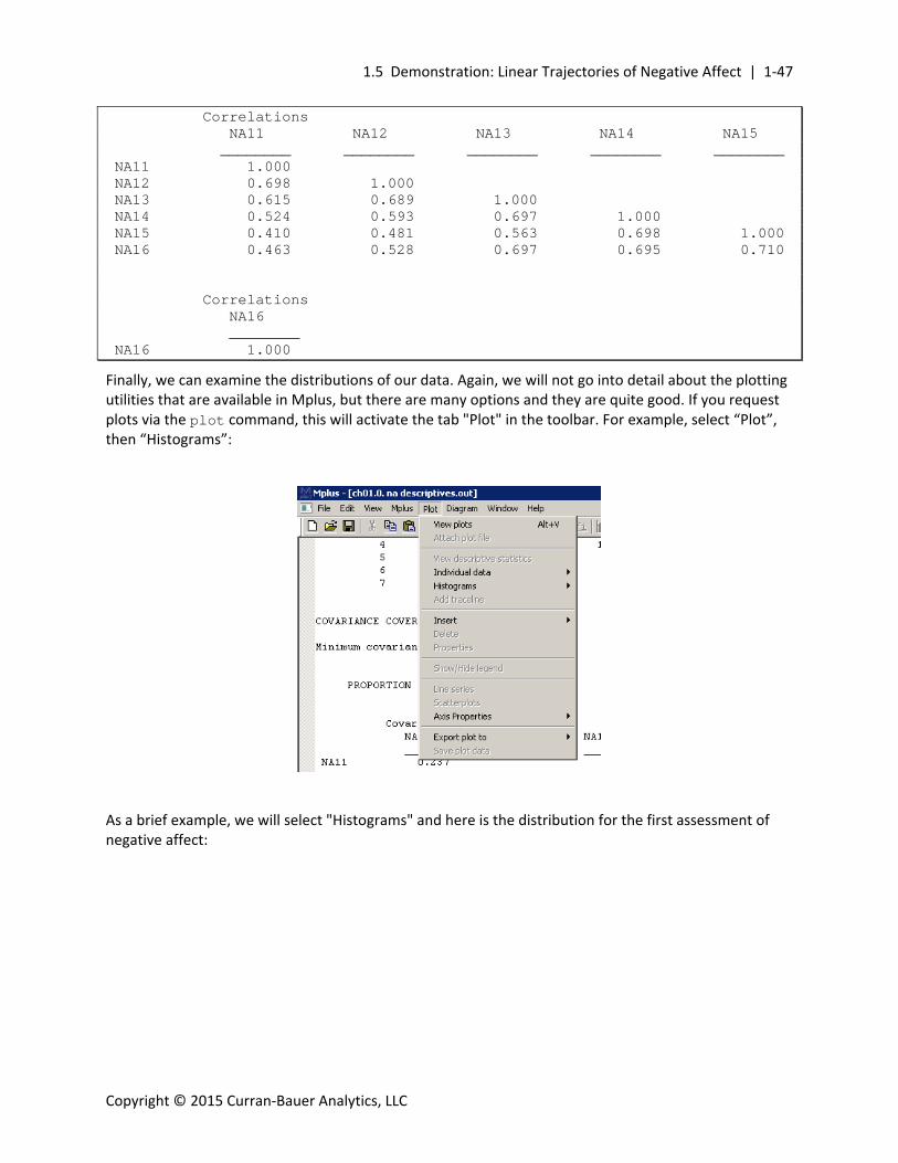
Correlations NA11 NA12 NA13 NA14 NA15 ________ ________ ________ ________ ________ NA11 1.000 NA12 0.698 1.000 NA13 0.615 0.689 1.000 NA14 0.524 0.593 0.697 1.000 NA15 0.410 0.481 0.563 0.698 1.000 NA16 0.463 0.528 0.697 0.695 0.710 Correlations NA16 ________ NA16 1.000

Finally, we can examine the distributions of our data. Again, we will not go into detail about the plotting utilities that are available in Mplus, but there are many options and they are quite good. If you request plots via the plot command, this will activate the tab "Plot" in the toolbar. For example, select “Plot”, then “Histograms”:

As a brief example, we will select "Histograms" and here is the distribution for the first assessment of negative affect:



We have done nothing to modify this plot, although there are many options for scaling and labeling these plots. Having examined our data, we will now move to fitting our first LCM.

Intercept‐onlyLCM,HeteroscedasticResiduals

We begin by fitting an intercept‐only model to the six repeated measures of negative affect. There are many different ways a latent curve model can be defined in Mplus. We will begin by using the simplest approach that is based on the vertical bar option (or "|") and allows for the efficient use of a number of defaults invoked by Mplus. We will demonstrate other approaches to defining these models as we move into more complex analyses. The path diagram for this model is:



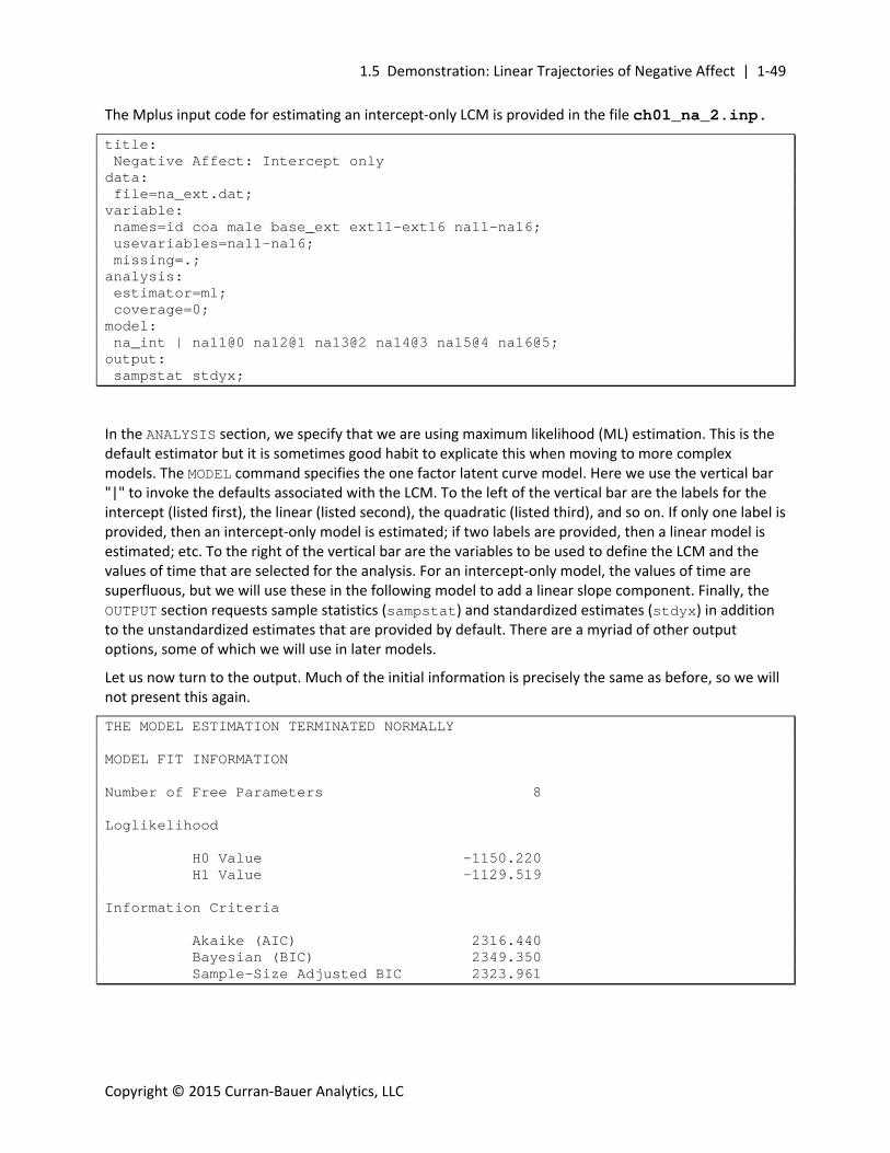
The Mplus input code for estimating an intercept‐only LCM is provided in the file ch01_na_2.inp.

title: Negative Affect: Intercept only data: file=na_ext.dat; variable: names=id coa male base_ext ext11-ext16 na11-na16; usevariables=na11-na16; missing=.; analysis: estimator=ml; coverage=0; model: na_int | na11@0 na12@1 na13@2 na14@3 na15@4 na16@5; output: sampstat stdyx;

In the ANALYSIS section, we specify that we are using maximum likelihood (ML) estimation. This is the default estimator but it is sometimes good habit to explicate this when moving to more complex models. The MODEL command specifies the one factor latent curve model. Here we use the vertical bar "|" to invoke the defaults associated with the LCM. To the left of the vertical bar are the labels for the intercept (listed first), the linear (listed second), the quadratic (listed third), and so on. If only one label is provided, then an intercept‐only model is estimated; if two labels are provided, then a linear model is estimated; etc. To the right of the vertical bar are the variables to be used to define the LCM and the values of time that are selected for the analysis. For an intercept‐only model, the values of time are superfluous, but we will use these in the following model to add a linear slope component. Finally, the OUTPUT section requests sample statistics (sampstat) and standardized estimates (stdyx) in addition to the unstandardized estimates that are provided by default. There are a myriad of other output options, some of which we will use in later models.

Let us now turn to the output. Much of the initial information is precisely the same as before, so we will not present this again.

THE MODEL ESTIMATION TERMINATED NORMALLY MODEL FIT INFORMATION Number of Free Parameters 8 Loglikelihood H0 Value -1150.220 H1 Value -1129.519 Information Criteria Akaike (AIC) 2316.440 Bayesian (BIC) 2349.350 Sample-Size Adjusted BIC 2323.961



Chi-Square Test of Model Fit Value 41.402 Degrees of Freedom 16 P-Value 0.0005 RMSEA (Root Mean Square Error Of Approximation) Estimate 0.059 90 Percent C.I. 0.037 0.082 Probability RMSEA <= .05 0.223 CFI/TLI CFI 0.953 TLI 0.965 Chi-Square Test of Model Fit for the Baseline Model Value 554.362 Degrees of Freedom 12 P-Value 0.0000 SRMR (Standardized Root Mean Square Residual) Value 0.115

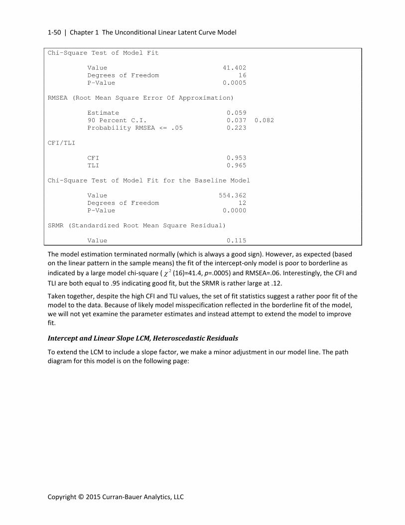
The model estimation terminated normally (which is always a good sign). However, as expected (based on the linear pattern in the sample means) the fit of the intercept‐only model is poor to borderline as

indicated by a large model chi‐square ( 2 (16)=41.4, p=.0005) and RMSEA=.06. Interestingly, the CFI and

TLI are both equal to .95 indicating good fit, but the SRMR is rather large at .12.

Taken together, despite the high CFI and TLI values, the set of fit statistics suggest a rather poor fit of the model to the data. Because of likely model misspecification reflected in the borderline fit of the model, we will not yet examine the parameter estimates and instead attempt to extend the model to improve fit.

InterceptandLinearSlopeLCM,HeteroscedasticResiduals

To extend the LCM to include a slope factor, we make a minor adjustment in our model line. The path diagram for this model is on the following page:



The code corresponding code is provided in ch01_na_3.inp.

title: Negative Affect: Intercept & slope, heteroscedastic errors data: file=na_ext.dat; variable: names=id coa male base_ext ext11-ext16 na11-na16; usevariables=na11-na16; missing=.; analysis: estimator=ml; coverage=0; model: na_int na_slp | na11@0 na12@1 na13@2 na14@3 na15@4 na16@5;

where we have simply added na_slp following na_int. This invokes additional defaults to estimate a linear slope factor with factor loadings set to 0, 1, 2, 3, 4, and 5; this slope factor is defined by a mean and variance and covaries with the intercept factor. All other code remains precisely the same as before. Examining more abbreviated model output, we see that the model achieves much improved fit:

Chi-Square Test of Model Fit Value 14.349 Degrees of Freedom 13 P-Value 0.3497 RMSEA (Root Mean Square Error Of Approximation) Estimate 0.015 90 Percent C.I. 0.000 0.050 Probability RMSEA <= .05 0.948



CFI/TLI CFI 0.998 TLI 0.998

The model chi‐square is non‐significant, the RMSEA is low, and the CFI and TLI are approaching their maxima. Recall from earlier that the intercept‐only model is nested within the linear model; that is, the intercept‐only model is equivalent to a linear growth model with the mean and variance of the latent slope factor, and the covariance between the intercept and the slope factor, all fixed to zero. As such, we can conduct a likelihood ratio test (LRT) to formally evaluate the improvement in model fit with the inclusion of the linear slope factor (see Appendix A for a review of this topic). The LRT is simply the difference between the model chi‐squares (41.4‐14.35=27.1) that is distributed on the difference between the model degrees‐of‐freedom (16‐13=3). A chi‐square of 27.1 distributed on df=3 is highly significant and indicates that there is a substantial improvement in model fit with the inclusion of the linear slope factor.

Prior to interpreting final parameter estimates, we can consider whether the model might support homoscedastic residuals. The unique time‐specific estimates for the heteroscedastic residuals are

Residual Variances NA11 0.152 0.040 3.804 0.000 NA12 0.136 0.024 5.577 0.000 NA13 0.156 0.021 7.434 0.000 NA14 0.158 0.021 7.401 0.000 NA15 0.193 0.027 7.223 0.000 NA16 0.163 0.041 3.927 0.000

Note that the estimates all seem to vary in the .14 to .19 range, suggesting that a single value could stand for all six time points. We will next impose an equality constraint on the time‐specific residual variances to ascertain whether the fewer parameters are needed to reproduce the observed data.

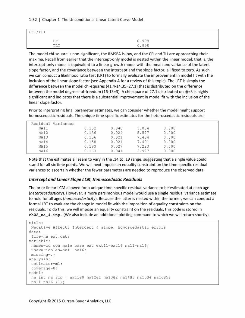
InterceptandLinearSlopeLCM,HomoscedasticResiduals

The prior linear LCM allowed for a unique time‐specific residual variance to be estimated at each age (heteroscedasticity). However, a more parsimonious model would use a single residual variance estimate to hold for all ages (homoscedasticity). Because the latter is nested within the former, we can conduct a formal LRT to evaluate the change in model fit with the imposition of equality constraints on the residuals. To do this, we will impose an equality constraint on the residuals; this code is stored in ch02_na_4.inp. (We also include an additional plotting command to which we will return shortly).

title: Negative Affect: Intercept & slope, homoscedastic errors data: file=na_ext.dat; variable: names=id coa male base_ext ext11-ext16 na11-na16; usevariables=na11-na16; missing=.; analysis: estimator=ml; coverage=0; model: na_int na_slp | na11@0 na12@1 na13@2 na14@3 na15@4 na16@5; na11-na16 (1);



plot: type=plot3; series=na11-na16 (*); output: sampstat stdyx;

In Mplus, listing a variable in the model statement without any brackets or parenthesis references the variance of that variable. In the prior models, the residuals of the repeated measures have been freely estimated by default (i.e., using the "|" command). We would now like to estimate these with the constraint that they be equal. To accomplish this, we do two things. First, we list the repeated measures separately to reference the residual variance; second, we assign a number in parenthesis to set those values to be equal. In Mplus, all parameters listed on a given line that share the same number in parenthesis are set to be equal. Thus, to set all of the residual variances to be equal, we add the line

na11-na16 (1);

Instead of estimating six separate residual variances (one for each unique age), we will obtain a single estimate of the residual variances that holds for all six ages. This model is nested within the prior model, so we can conduct an LRT to formally evaluate whether one residual variance estimate is sufficient to hold for all six time points.

The chi‐square for the linear LCM with homoscedasticity is

Chi-Square Test of Model Fit Value 17.395 Degrees of Freedom 18 P-Value 0.4961

Recall that the chi‐square for the previous model with heteroscedasticity was


As expected, the LCM with homoscedasticity has 5 fewer parameters than the LCM with heteroscedasticity (because one parameter is needed for the residuals in the former and six parameters are needed in the latter). The difference in chi‐square statistics is 17.395‐14.349=3.046 that is distributed on df=18‐13=5 and is non‐significant (p=.31; note that we must determine this probability value based on the chi‐square difference and df outside of Mplus). We can conclude that increasing the model parsimony by estimating just a single residual variance for all six ages does not lead to a significant reduction in model fit; that is, the model fits no worse with one residual variance compared to six residual variances. We thus retain this model simplification and can examine our final results.

To begin, the model fits the data quite well, with all indices indicating excellent fit:




RMSEA (Root Mean Square Error Of Approximation) Estimate 0.000 90 Percent C.I. 0.000 0.040 Probability RMSEA <= .05 0.989 CFI/TLI CFI 1.000 TLI 1.001 SRMR (Standardized Root Mean Square Residual) Value 0.050

We can next examine the parameter estimates and standard errors (we only present a subset of the output here):

MODEL RESULTS Two-Tailed Estimate S.E. Est./S.E. P-Value NA_INT | NA11 1.000 0.000 999.000 999.000 NA12 1.000 0.000 999.000 999.000 NA13 1.000 0.000 999.000 999.000 NA14 1.000 0.000 999.000 999.000 NA15 1.000 0.000 999.000 999.000 NA16 1.000 0.000 999.000 999.000 NA_SLP | NA11 0.000 0.000 999.000 999.000 NA12 1.000 0.000 999.000 999.000 NA13 2.000 0.000 999.000 999.000 NA14 3.000 0.000 999.000 999.000 NA15 4.000 0.000 999.000 999.000 NA16 5.000 0.000 999.000 999.000

Because the intercept and slope factor loadings are set to predetermined values, these have no standard errors and Mplus reports 999.000 for critical ratios and p‐values; this is perfectly fine and is exactly how we've set up the model.

NA_SLP WITH NA_INT -0.035 0.019 -1.842 0.065

The covariance of the intercept and slope is negative and marginally significant ( 21ˆ .035 ); we'll see

in the standardized output later in the program that this translates into a correlation of .39r . The substantive interpretation is that adolescents who reporter higher initial levels of negative affect to tend decrease more rapidly over time (and vice versa). Care should be taken when interpreting these covariances because they are directly influenced by where the zero‐point is placed when coding time. As we would fully expect based on how the intercept is defined, this covariance would likely be quite different if the zero‐point were placed at the middle or at the end of the growth process.



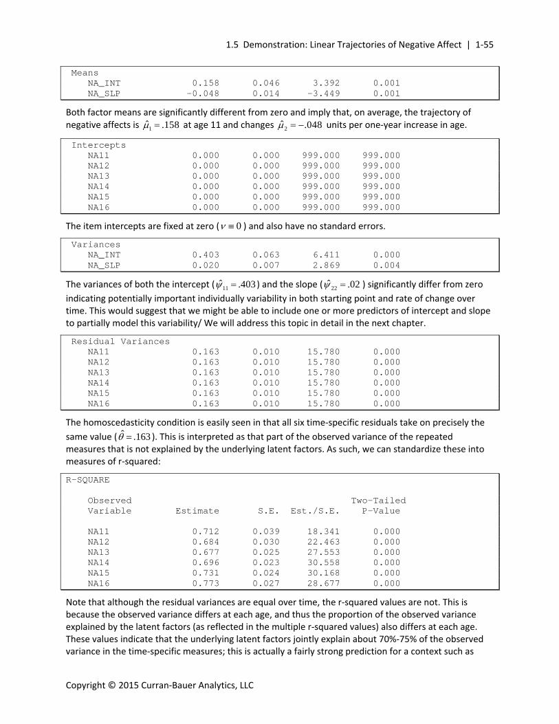
Means NA_INT 0.158 0.046 3.392 0.001 NA_SLP -0.048 0.014 -3.449 0.001

Both factor means are significantly different from zero and imply that, on average, the trajectory of negative affects is 1ˆ .158 at age 11 and changes 2ˆ .048 units per one‐year increase in age.

Intercepts NA11 0.000 0.000 999.000 999.000 NA12 0.000 0.000 999.000 999.000 NA13 0.000 0.000 999.000 999.000 NA14 0.000 0.000 999.000 999.000 NA15 0.000 0.000 999.000 999.000 NA16 0.000 0.000 999.000 999.000

The item intercepts are fixed at zero ( 0 ) and also have no standard errors.

Variances NA_INT 0.403 0.063 6.411 0.000 NA_SLP 0.020 0.007 2.869 0.004

The variances of both the intercept ( 11ˆ .403 ) and the slope ( 22ˆ .02 ) significantly differ from zero

indicating potentially important individually variability in both starting point and rate of change over time. This would suggest that we might be able to include one or more predictors of intercept and slope to partially model this variability/ We will address this topic in detail in the next chapter.

Residual Variances NA11 0.163 0.010 15.780 0.000 NA12 0.163 0.010 15.780 0.000 NA13 0.163 0.010 15.780 0.000 NA14 0.163 0.010 15.780 0.000 NA15 0.163 0.010 15.780 0.000 NA16 0.163 0.010 15.780 0.000

The homoscedasticity condition is easily seen in that all six time‐specific residuals take on precisely the

same value ( ˆ .163 ). This is interpreted as that part of the observed variance of the repeated measures that is not explained by the underlying latent factors. As such, we can standardize these into measures of r‐squared:

R-SQUARE Observed Two-Tailed Variable Estimate S.E. Est./S.E. P-Value NA11 0.712 0.039 18.341 0.000 NA12 0.684 0.030 22.463 0.000 NA13 0.677 0.025 27.553 0.000 NA14 0.696 0.023 30.558 0.000 NA15 0.731 0.024 30.168 0.000 NA16 0.773 0.027 28.677 0.000

Note that although the residual variances are equal over time, the r‐squared values are not. This is because the observed variance differs at each age, and thus the proportion of the observed variance explained by the latent factors (as reflected in the multiple r‐squared values) also differs at each age. These values indicate that the underlying latent factors jointly explain about 70%‐75% of the observed variance in the time‐specific measures; this is actually a fairly strong prediction for a context such as



child development. This could be in part indicative of the rather high reliability of the repeated measures that were scored using a rigorous item response theory modeling approach.

Finally, recall that we included a plot function that allows us to examine the observed vs. fitted mean trajectory. To review, the new code was

plot: type=plot3; series=na11-na16 (*);

The key line here is series=na11-na16 (*) which requests that means be plotted for negative affect from ages 11 and 16, and the asterisk invokes the default that time be coded from 0 to 5 by 1. Again, there are many variants of these plots; here we simply want to see the model‐implied mean trajectory.

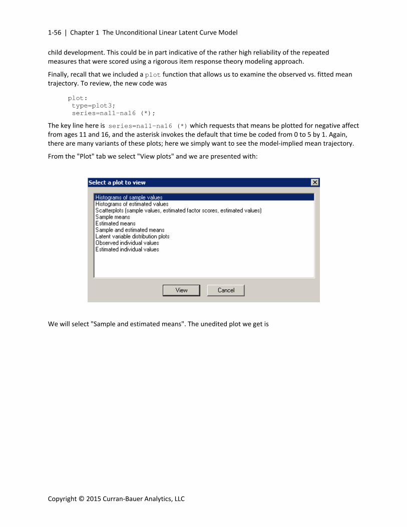
From the "Plot" tab we select "View plots" and we are presented with:

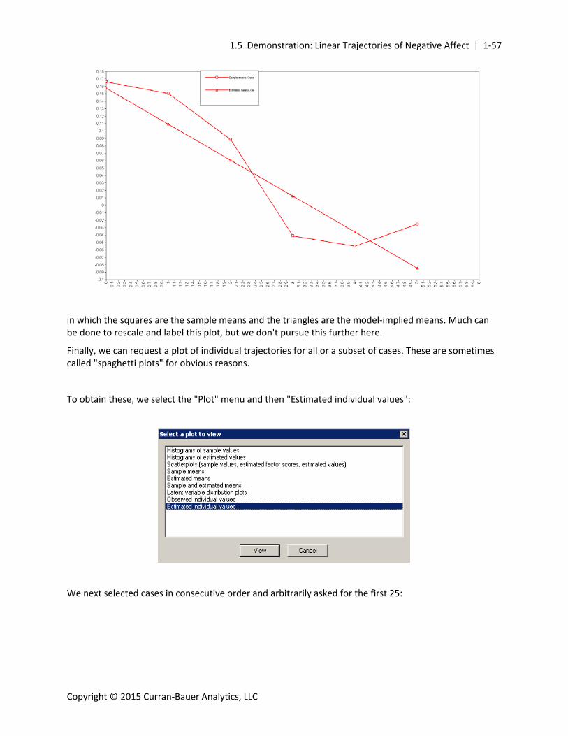
We will select "Sample and estimated means". The unedited plot we get is



in which the squares are the sample means and the triangles are the model‐implied means. Much can be done to rescale and label this plot, but we don't pursue this further here.

Finally, we can request a plot of individual trajectories for all or a subset of cases. These are sometimes called "spaghetti plots" for obvious reasons.

To obtain these, we select the "Plot" menu and then "Estimated individual values":

We next selected cases in consecutive order and arbitrarily asked for the first 25:



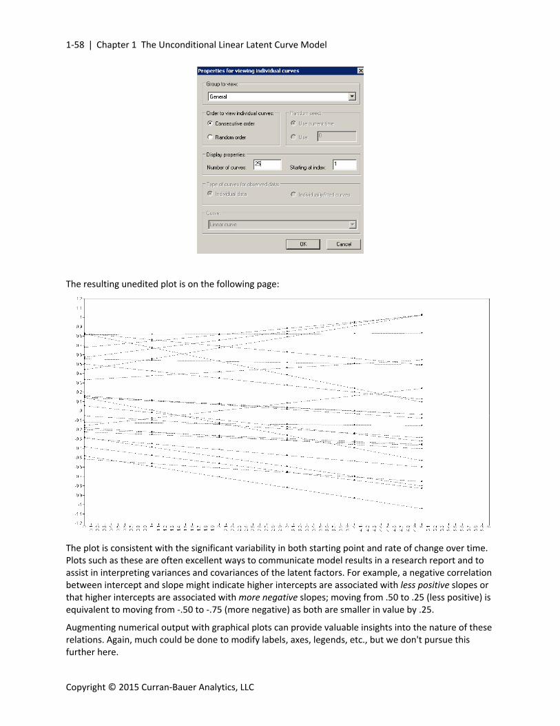
The resulting unedited plot is on the following page:

The plot is consistent with the significant variability in both starting point and rate of change over time. Plots such as these are often excellent ways to communicate model results in a research report and to assist in interpreting variances and covariances of the latent factors. For example, a negative correlation between intercept and slope might indicate higher intercepts are associated with less positive slopes or that higher intercepts are associated with more negative slopes; moving from .50 to .25 (less positive) is equivalent to moving from ‐.50 to ‐.75 (more negative) as both are smaller in value by .25.

Augmenting numerical output with graphical plots can provide valuable insights into the nature of these relations. Again, much could be done to modify labels, axes, legends, etc., but we don't pursue this further here.



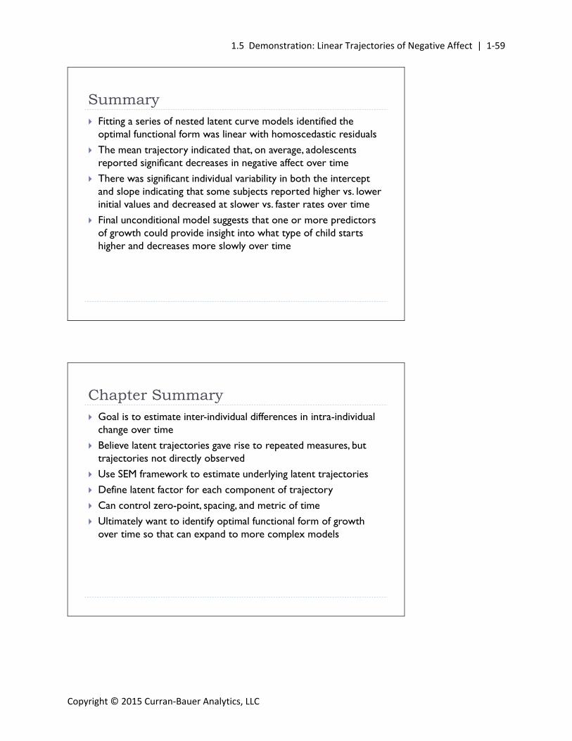
Summary Fitting a series of nested latent curve models identified the

optimal functional form was linear with homoscedastic residuals

The mean trajectory indicated that, on average, adolescents reported significant decreases in negative affect over time

There was significant individual variability in both the intercept and slope indicating that some subjects reported higher vs. lower initial values and decreased at slower vs. faster rates over time

Final unconditional model suggests that one or more predictors of growth could provide insight into what type of child starts higher and decreases more slowly over time

Chapter Summary Goal is to estimate inter-individual differences in intra-individual

change over time

Believe latent trajectories gave rise to repeated measures, but trajectories not directly observed

Use SEM framework to estimate underlying latent trajectories

Define latent factor for each component of trajectory

Can control zero-point, spacing, and metric of time

Ultimately want to identify optimal functional form of growth over time so that can expand to more complex models

chapter 1 the unconditional linear latent curve model€¦ · the unconditional linear latent curve...

Documents