1

CHAPTER 10

ELECTROMAGNETIC INDUCTION

10.1 Introduction

In 1820, Oersted had shown that an electric current generates a magnetic field. But can a magnetic

field generate an electric current? This was answered almost simultaneously and independently in

1831 by Joseph Henry in the United States and Michael Faraday in Great Britain. Faraday

constructed an iron ring, about six inches in diameter. He wound two coils of wire tightly around

the ring; one coil around one half (semicircle) of the ring, and the second coil around the second

half of the ring. The two coils were not connected to one another other than by sharing the same

iron core. One coil (which I'll refer to as the "primary" coil) was connected to a battery; the other

coil (which I'll refer to as the "secondary" coil) was connected to a galvanometer. When the battery

was connected to the primary coil a current, of course, flowed through the primary coil. This

current generated a magnetic field throughout the iron core, so that there was a magnetic field

inside each of the two coils. As long as the current in the primary coil remained constant, there was

no current in the secondary coil. What Faraday observed was that at the instant when the battery

was connected to the primary, and during that brief moment when the current in the primary was

rising from zero, a current momentarily flowed in the secondary – but only while the current in the

primary was changing. When the battery was disconnected, and during the brief moment when the

primary current was falling to zero, again a current flowed in the secondary (but in the opposite

direction to previously). Of course, while the primary current was changing, the magnetic field in

the iron core was changing, and Faraday recognized that a current was generated in the secondary

while the magnetic flux through it was changing. The strength of the current depended on the

resistance of the secondary, so it is perhaps more fundamental to note that when the magnetic flux

through a circuit changes, an electromotive force (EMF) is generated in the circuit, and the faster

the flux changes, the greater the induced EMF. Quantitative measurements have long established

that:

While the magnetic flux through a circuit is changing, an EMF is generated in the circuit

which is equal to the rate of change of magnetic flux BΦ& through the circuit.

This is generally called "Faraday's Law of Electromagnetic Induction". A complete statement of

the laws of electromagnetic induction must also tell us the direction of the induced EMF, and this is

generally given in a second statement usually known as "Lenz's Law of Electromagnetic

Induction", which we shall describe in Section 10.2. When asked, therefore, for the laws of

electromagnetic induction, both laws must be given: Faraday's, which deals with the magnitude of

the EMF, and Lenz's, which deals with its direction.

You will note that the statement of Faraday's Law given above, says that the induced EMF is not

merely "proportional" to the rate of change of magnetic B-flux, but is equal to it. You will

therefore want to refer to the dimensions of electromotive force (SI unit: volt) and of B-flux (SI

unit: weber) and verify that BΦ& is indeed dimensionally similar to EMF. This alone does not tell

you the constant of proportionality between the induced EMF and BΦ& , though the constant is in

2

fact unity, as stated in Faraday's law. You may then ask: Is this value of 1 for the constant of

proportionality between the EMF and BΦ& an experimental value (and, if so, how close to 1 is it,

and what is its currently determined best value), or is it expected theoretically to be exactly 1?

Well, I suppose it has to be admitted that physics is an experimental science, so that from that point

of view the constant has to be determined experimentally. But I shall advance an argument shortly

to show not only that you would expect it to be exactly 1, but that the very phenomenon of

electromagnetic induction is only to be expected from what we already knew (before embarking

upon this chapter) about electricity and magnetism.

Incidentally, we recall that the SI unit for ΦB is the weber (Wb). To some, this is not a very

familiar unit and some therefore prefer to express ΦB in T m2. Yet again, consideration of

Faraday's law tells us that a perfectly legitimate SI unit (which many prefer) for ΦB is V s.

10.2 Electromagnetic Induction and the Lorentz Force

Imagine that there is a uniform magnetic field directed into the plane of the paper (or your

computer screen), as in figure X.1. Suppose there is a metal rod, as in the figure, and that the rod is

being moved steadily to the right. We know that, within the metal, there are many free conduction

electrons, not attached to any particular atom, but free to wander about inside the metal. As the

metal rod is moved to the right, these free conduction electrons are also moving to the right and

therefore they experience a Lorentz q v %%%% B force, which moves them down (remember – electrons

are negatively charged) towards the bottom end of the rod. Thus the movement of the rod through

the magnetic field induces a potential difference across the ends of the rod. We have achieved

electromagnetic induction, and, seen this way, there is nothing new: electromagnetic induction is

nothing more than the Lorentz force on the conduction electrons within the metal.

You may speculate that, as an aircraft flies through Earth's magnetic field, a potential difference

will be induced across the wingtips. You might try to imagine how you might set up an experiment

to detect or measure this. You might also speculate that, as seawater flows up the English Channel,

a potential difference is induced between England and France. You might also ask yourself: What

if the rod were stationary, and the magnetic field were moving to the left? That's an interesting

1 1 1 1 1

1 1 1 1 1

1 1 1 1 1

1 1 1 1 1

1 1 1 1 1

FIGURE X.1

B

3

discussion for lunchtime: Can you imagine the magnetic field moving to the left? Who's to say

whether the rod or the field is moving?

If we were somehow to connect the ends of the rod in figure X.1 to a closed circuit, we might cause

a current to flow – and we would then have made an electric generator. Look at figure X.2.

We imagine that our metal bar is being pulled steadily to the right at speed v, and that it is in

contact with, and sliding smoothly without friction upon, two rails a distance a apart, and that the

rails are connected via a resistance R. As a consequence, a current I flows in the circuit in the

direction shown, counterclockwise. (The current is, of course, made up of negative conduction

electrons moving clockwise.) Now the magnetic field will exert a force on the current in the rod.

The force on the rod will be a I %%%% B; that is aIB acting to the left. In order to keep the rod moving

steadily at speed v to the right against this force, work will have to be done at a rate aIBv . The

work will be dissipated in the resistance at a rate I V where V is the induced EMF. Therefore the

induced EMF is Bav. But av is the rate at which the area of the circuit is increasing, and Bav is the

rate at which the magnetic B-flux through the circuit is increasing. Therefore the induced EMF is

equal to the rate of change of magnetic flux through the circuit. Thus we have predicted Faraday's

law quantitatively merely from what we already know about the forces on currents and charged

particles in a magnetic field.

10.3 Lenz's Law

We can now address ourselves to the direction of the induced EMF. From our knowledge of the

Lorentz force q v %%%% B we see that the current flows counterclockwise, and that this results in a force

on the rod that is in the opposite direction to its motion. But, even if we did not know this law, or

had forgotten the formula, or if we didn't understand a vector product, we could see that this must

be so. For, suppose that we move the rod to the right, and that, as a consequence, there will be a

force also the right. Then the rod moves faster, and the force to the right is greater, and the rod

moves yet faster, and so on. The rod would accelerate indefinitely, for the expenditure of no work.

No – this cannot be right. The direction of the induced EMF must be such as to oppose the change

of flux that causes it. This is merely a consequence of conservation of energy, and it can be stated

as Lenz's Law:

FIGURE X.2

a

1 1 1 1 1

1 1 1 1 1

1 1 1 1 1

1 1 1 1 1

1 1 1 1 1

B

1 1 1 1 1

1 1 1 1 1

1 1 1 1 1

1 1 1 1 1

1 1 1 1 1

R x&

I

4

When an EMF is induced in a circuit as a result of changing magnetic flux through the

circuit, the direction of the induced EMF is such as to oppose the change of flux that causes it.

In our example of Section 10.2, we increased the magnetic flux through a circuit by increasing the

area of the circuit. There are other ways of changing the flux through a circuit. For example, in

figure X.3, we have a circular wire and a magnetic field perpendicular to the plane of the circle,

directed into the plane of the drawing.

We could increase the magnetic flux through the coil by increasing the strength of the field rather

than by increasing the area of the coil. The rate of increase of the flux would then be BA & rather

than .BA& We could imagine increasing B, for example by moving a magnet closer to the coil, or

by moving the coil into a region where the magnetic field was stronger; or, if the magnetic field is

generated by an electromagnet somewhere, by increasing the current in the electromagnet. One

way or another, we increase the strength of the field through the coil. An EMF is generated in the

coil equal to the rate of change of magnetic flux, and consequently a current flows in the coil. In

which direction does this induced current flow? It flows in such a direction as to oppose the

increase in B that causes it. That is, the current flows counterclockwise in the coil. If this were not

so, and the induced current were clockwise, this would still further increase the flux through the

coil, and the current would increase further, and the flux would increase further, and so on. A

runaway increase in the current and the field would result, and energy would not be conserved.

If we were in decrease the strength of the field through the coil, a current would flow clockwise in

the coil – i.e. in such a sense as to tend to increase the field – i.e. to oppose the decrease in field that

we are trying to impose. It may well occur to you at this stage that it is impossible to increase the

current in a circuit instantaneously, and it takes a finite time to establish a new level of current.

This is correct – a point to which we shall return later, when indeed we shall calculate just how

long it does take.

Another way in which we could change the magnetic flux through a coil would be to rotate the coil

in a magnetic field. For example, in figure X.4a, we see a magnetic field directed to the right, and a

coil whose normal is perpendicular to the field. There is no magnetic flux through the coil. If we

now rotate the coil, as in figure X.4b, the flux through the coil will increase, an EMF will be

induced in the coil, equal to the rate of increase of flux, and a current will flow. The current will

flow in a direction such that the magnetic moment of the coil will be as shown, which will result in

an opposition to our imposed rotation on the coil, and the current will flow in the direction

indicated by the symbols ? and 1.

FIGURE X.3 1

B

5

If the flux through a coil changes at a rate ,BΦ& and if the coil is not just a single turn but is made of

N turns, the induced EMF will be BΦ& per turn, so that the induced EMF in the coil as a whole will

be .BΦ&N

10.4 Ballistic Galvanometer and the Measurement of Magnetic Field

A galvanometer is similar to a sensitive ammeter, differing mainly in that when no current passes

through the meter, the needle is in the middle of the dial rather than at the left hand end. A

galvanometer is used not so much to measure a current, but rather to detect whether or not a current

is flowing, and in which direction. In the ballistic galvanometer, the motion of the needle is

undamped, or as close to undamped as can easily be achieved. If a small quantity of electricity is

passed through the ballistic galvanometer in a time that is short compared with the period of

oscillation of the needle, the needle will jerk from its rest position, and then swing to and fro in

lightly damped harmonic motion. (It would be simple harmonic motion if it could be completely

undamped.) The amplitude of the motion, or rather the extent of the first swing, depends on the

quantity of electricity that was passed through the galvanometer. It could be calibrated, for

example, by discharging various capacitors through it, and making a table or graph of amplitude of

swing versus quantity of electricity passed.

Now, if we have a small coil of area A, N turns, resistance R, we could place the coil perpendicular

to a magnetic field B, and then connect the coil to a ballistic galvanometer. Then, suddenly (in a

time that is short compared with the oscillation period of the galvanometer), remove the coil from

the field (or rotate it through 90o) so that the flux through the coil goes from AB to zero. While the

FIGURE X.4

(a) (b)

????

1111

ω

6

flux through the coil is changing, and EMF will be induced, equal to ,BNA & and consequently a

current will flow momentarily through the coil of magnitude

,)/( rRBNAI += & 10.4.1

where r is the resistance of the galvanometer. Integrate this with respect to time, with initial

condition Q = 0 when t = 0, and we find for the total quantity of electricity that flows through the

galvanometer

Q NAB R r= +/( ) . 10.4.2

Since Q can be measured from the amplitude of the galvanometer motion, the strength of the

magnetic field, B is determined.

I mentioned that the ballistic galvanometer differs from that of an ordinary galvanometer or

ammeter in that its motion is undamped. The motion of the needle in an ordinary ammeter is

damped, so that the needle doesn't swing violently whenever the current is changed, and so that the

needle moves promptly and purposefully towards its correct position. How is this damping

achieved?

The coil of a moving-coil meter is wound around a small aluminium frame called a former. When

the current through the ammeter coil is changed, the coil – and the former – swing round; but a

current is induced in the former, which gives the former a magnetic moment in such a sense as to

oppose and therefore dampen the motion. The resistance of the former is made just right so that

critical damping is achieved, so that the needle reaches its equilibrium position in the least time

without overshoot or swinging. The little aluminium former does not look as if it were an

important part of the instrument – but in fact its careful design is very important!

10.5 AC Generator

This and the following sections will be devoted to generators and motors. I shall not be concerned

with – and indeed am not knowledgeable about – the engineering design or practical details of real

generators or motors, but only with the scientific principles involved. The "generators" and

"motors" of this chapter will be highly idealized abstract concepts bearing little obvious

resemblance to the real things. Need an engineering student, then, pay any attention to this? Well,

of course, all real generators and motors obey and are designed around these very scientific

principles, and they wouldn't work unless their designers and builders had a very clear knowledge

and understanding of the basic principles.

The rod sliding on rails in a magnetic field described in Section 10.2 in fact was a D.C. (direct

current) generator. I now describe an A.C. (alternating current) generator.

In figure X.5 we have a magnetic field B, and inside the field we have a coil of area A (yes – area is

a vector) and N turns. The coil is being physically turned counterclockwise by some outside

agency at an angular speed ω radians per second. I am not concerned with who, what or how it is

7

being physically turned. For all I know, it might be turned by a little man turning a hand crank, or

by a steam turbine driven by a coal- or oil-burning plant, or by a nuclear reactor, or it might be

driven by a water turbine from a hydroelectric generating plant, or it might be turned by having

something rubbing against the rim of your bicycle wheel. All I am interested in is that it is being

mechanically turned at an angular speed ω. As the coil turns, the flux through it changes, and a

current flows through the coil in a direction such that the magnetic moment generated for the coil is

in the direction indicated for the area A in figure X.5, and also indicated by the symbols ? and 1.

This will result in an opposition to rotation of the coil; whoever or whatever is causing the coil to

rotate will experience some opposition to his efforts and will have to do work. You can also

deduce the direction of the induced current by considering the direction of the Lorentz force on the

electrons in the wire of the coil.

At the instant illustrated in figure X.5, the flux through the coil is AB cos ,θ or AB tcos ,ω if we

assume that θ = 0 at t = 0. The rate of change of flux through the coil at this instant is the time

derivative of this, or − AB tω ωsin . The magnitude of the induced EMF is therefore

,sinˆsin tVtNABV ω=ωω= 10.5.1

where V (" V-peak") is the peak or maximum EMF, given by

.ˆ ω= NABV 10.5.2

Are you surprised that the peak EMF is proportional to N ? To A ? To B ? To ω ? Verify that

NAB ω has the correct dimensions for V .

The peak EMF occurs when the flux through the coil is changing most rapidly; this occurs when

θ = 90o , at which time the coil is horizontal and the flux through it is zero.

A

????

1111

ω

B θ

FIGURE X.5

8

The leads from the coil can be connected to an external circuit via a pair of slip rings through

which they can deliver current to the circuit.

The actual physical design of a generator is beyond the scope of this chapter and indeed of my

expertise, though all depend on the physical principles herein described. In the "design" (such as it

is) that I have described, the coil in which the EMF is induced is the rotor while the magnet is the

stator – but this need not always be the case, and indeed designs are perfectly possible in which the

magnet is the rotor and the coil the stator. In my design, too, I have assumed that there is but one

coil – but there might be several in different planes. For example, you might have three coils

whose planes make angles of 120o with each other. Each then generates a sinusoidal voltage, but

the phase of each differs by 120o from the phases of the other two. This enables the delivery of

power to three circuits. In a common arrangement these three circuits are not independent, but each

is connected to a common line. The EMF in this common line is then made up three sine waves

differing in phase by 120o :

.)]240sin()120sin([sinˆ oo +ω++ω+ω= tttVV 10.5.3

There are several ways in which you can see what this is like. For example, you could calculate

this expression for numerous values of t and plot the function out as a graph. Or you could expand

the expressions V t= +sin( )ω 120o and V t= +sin( )ω 240o , and gather the various terms

together to see what you get. (I recommend trying this.) Or you could simply add the three

components in a phase diagram:

FIGURE X.6

9

It then becomes obvious that the sum is zero, and this line is the neutral line, the other three being

live lines.

10.6 AC Power

When a current I flows through a resistance R, the rate of dissipation of electrical energy as heat is

I R2 . If an alternating potential difference tVV ω= sinˆ is applied across a resistance, then an

alternating current tII ω= sinˆ will flow through it, and the rate at which energy is dissipated as

heat will also change periodically. Of interest is the average rate of dissipation of electrical energy

as heat during a complete cycle of period P = 2π ω/ .

Let W = instantaneous rate of dissipation of energy, and W = average rate over a cycle of period

P = 2π ω/ . Then

dttIRdtIRWdtPWPPP

∫∫∫ ω===0

22

0

2

0sinˆ

.ˆ]2sin[ˆ)2cos1(ˆ 2

21/2

0212

21

0

2

21 PIRttIRdttIR

PP=ω−=ω−= ωπ=

ω∫ 10.6.1

Thus .ˆ2

21 IRW = 10.6.2

The expression 2

21 I is the mean value of I

2 over a complete cycle. Its square root II ˆ707.02/ˆ =

is the root mean square value of the current, IRMS. Thus the average rate of dissipation of electrical

energy is

W RI= RMS

2 . 10.6.3

Likewise, the RMS EMF (pardon all the abbreviations) over a complete cycle is .2/V

Often when an AC current or voltage is quoted, it is the RMS value that is meant rather than the

peak value. I recommend that in writing or conversation you always make it explicitly clear which

you mean.

Also of interest is the mean induced voltage V over half a cycle. (Over a full cycle, the mean

voltage is, of course, zero.) We have

02/

0

2/

0 22

][cosˆ

sinˆ2/ π=ω

ω=ω== ∫∫ Pt

VdttVdtVPV

PP

.ˆ2

)cos1(ˆ

ω=π−

ω=

VV 10.6.4

10

Remembering that P = 2π ω/ , we see that

.9003.022ˆ6366.0

ˆ2RMS

RMS VV

VV

V =π

==π

= 10.6.5

10.7 Linear Motors and Generators

Most (but not all!) real motors and generators are, of course, rotary. In this section I am going to

describe highly idealized and imaginary linear motors and generators, only because the geometry is

simpler than for rotary motors, and it is easier to explain certain principles. We'll move on the

rotary motors afterwards.

In figure X.7 I compare a motor and a generator. In both cases there is supposed to be an external

magnetic field (from some external magnet) directed away from the reader. A metal rod is resting

on a pair of conducting rails.

1 B v I

R

E

MOTOR

1 B v I

GENERATOR

FIGURE X.7

B

11

In the motor, a battery is connected in the circuit, causing a current to flow clockwise around the

circuit. The interaction between the current and the external magnetic field produces a force on the

rod, moving it to the right.

In the generator, the rod is moved to the right by some externally applied force, and a current is

induced counterclockwise. If the B inside the circle represents a light bulb, a current will flow

through the bulb, and the bulb will light up.

Let us suppose that the rails are smooth and frictionless, and suppose that, in the motor, the rod isn't

pulling any weight. That is to say, suppose that there is no mechanical load on the motor. How fast

will the rod move? Since there is a force moving the rod to the right, will it continue to accelerate

indefinitely to the right, with no limit to its eventual speed? No, this is not what happens. When

the switch is first closed and the rod is stationary, a current will flow, given by E = IR, where E is

the EMF of the battery and R is the total resistance of the circuit. However, when the rod has

reached a speed v, the area of the circuit is increasing at a rate av, and a back EMF (which opposes

the EMF of the battery), of magnitude avB is induced, so the net EMF in the circuit is now

BaE v− and the current is correspondingly reduced according to

E a B IR− =v . 10.7.1

Eventually the rod reaches a limiting speed of E aB/ ( ) , at which point no further current is being

taken from the battery, and the rod (sliding as it is on frictionless rails with no mechanical load)

then obeys Newton's first law of motion – namely it will continue in its state of uniform motion,

because no forces are no acting upon it.

Problem 1. Show that the speed increases with time according to

,)(

exp12

−−=

mR

tBa

aB

Ev 10.7.2

where m is the mass of the rod.

Problem 2. Show that the time for the rod to reach half of its maximum speed is

tmR

a B1 2 2

2/

ln

( ).= 10.7.3

Problem 3. Suppose that E = 120 V, a = 1.6 m , m = 1.92 kg and R = 4 Ω . If the rod reaches a

speed of 300 m s−1

in 300 s, what is the strength of the magnetic field?

I'll give solutions to these problems at the end of this section. Until then – no peeking.

12

In a frictionless rotary motor, the situation would be similar. Initially the current would be E/R, but,

when the motor is rotating with angular speed ω, the average back EMF is 2 NAB ω π/ equation

10.5.5), and by the time this has reached the EMF of the battery, the frictionless, loadless coil

carries on rotating at constant angular speed, taking no current from the battery.

Now let's go back to our linear motor consisting of a metal rod lying on two rails, but this time

suppose that there is some mechanical resistance to the motion. This could be either because there

is friction between the rod and the rails, or perhaps the rod is dragging a heavy weight behind it, or

both. One way or another, let us suppose that the rod is subjected to a constant force F towards the

left. As before, the relation between the current and the speed is given by equation 10.7.1, but,

when a steady state has been reached, the electromagnetic force aIB pulling the rod to the right is

equal to the mechanical load F dragging the rod to the left. That is, E a B IR− =v and F a I B= .

If we eliminate I between these two equations, we obtain

E a BFR

aB− =v , 10.7.4

or v = −E

a B

R

a BF

( ).

2 10.7.5

This equation, which relates the speed at which the motor runs to the mechanical load, is called the

motor performance characteristic. In our particular motor, the performance characteristic shows

that the speed at which the motor runs decreases steadily as the load is increased, and the motor

runs to a grinding halt for a load equal to a B E R/ . (Verify that this has the dimensions of force.)

The current is then E/R. This current may be quite large. If you physically prevent a real motor

from turning by applying a mechanical torque to it so large that the motor cannot move, a large

current will flow through the coil – large enough to heat and possibly fuse the coil. You will hear a

sharp crack and see a little puff of smoke.

If we multiply equation 10.7.6 by I, we obtain

E I a I B I R= +v 2 , 10.7.6

or E I F I R= +v 2 . 10.7.7

This shows that the power produced by the battery goes partly into doing external mechanical

work, and the remainder is dissipated as heat in the resistance. Restrain the motor so that v = 0,

and all of that E I goes into I 2R.

If you were physically to move the rod to the right at a speed faster than the equilibrium speed, the

back EMF becomes greater than the battery EMF, and current flows back into the battery. The

device is then a generator rather than a motor.

The nature of the performance characteristic varies with the details of motor design. You may not

want a motor whose speed decreases so drastically with load. You may have to decide in advance

13

what sort of performance characteristic you want the motor to have, depending on what tasks you

want it to perform, and then you have to design the motor accordingly. We shall mention some

possibilities in the next section.

Now – the promised solutions to the problems.

Solution to Problem 1.

When the speed of the rod is v, the net EMF in the circuit is E a B− v , so the current

is( ) /E a B R− v , and so the force on the rod will be aB E a B R( ) /− v and the acceleration d dtv /

will be aB E a B mR( ) /( ) .− v The equation of motion is therefore

.dtmR

aB

aBE

d=

− v

v 10.7.8

Integration, with v = 0 when t = 0, gives the required equation 10.7.2.

Solution to Problem 2.

Just put v =E

a B2 in equation 10.7.2 and solve for t. Verify that the expression has the dimensions

of time.

Solution to Problem 3.

Put the given numbers into equation 10.7.2 to get

B e B= − −14

10012

( ) 10.7.9

and solve this for B. (Nice and easy. But if you are not experienced in solving equations such as

this, the Newton-Raphson process is described in Chapter 1 of the Celestial Mechanics notes of this

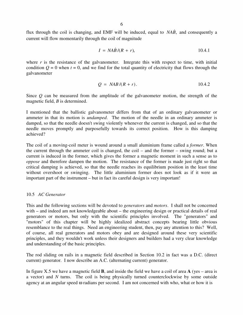
series. This equation would be good practice.) There are two possible answers, namely 0.043996

and 0.249505 teslas. I draw the speed:time graphs for the two solutions below:

14

0 500 1000 15000

200

400

600

800

1000

1200

Time s

Sp

ee

d

m s

-1

Numbers of interest for the two fields:

B (T) ∞v (m s−1

) t s

0.0440 1704.7 1074.29

0.2495 300.6 33.40

10.8 Rotary Motors

Most real motors, of course, are rotary motors, though all of the principles described for our highly

idealized linear motor of the previous section still apply.

Current is fed into a coil (known as the armature) via a split-ring commutator and the coil therefore

develops a magnetic moment. The coil is in a magnetic field, and it therefore experiences a torque.

(Figure X.5) The coil rotates and soon its magnetic moment vector will be parallel to the field and

there would be no further torque – except that, at that instant, the split-ring commutator reverses the

direction of the current in the coil, and hence reverses the direction of the magnetic moment. Thus

the coil continues to rotate until, half a period later, its new magnetic moment again lines up with

the magnetic field, and the commutator again reverses the direction of the moment.

15

As in the case of the linear motor, the coil reaches a maximum angular speed, which depends on the

mechanical load (this time a torque). and the relation between the maximum angular speed and the

torque is the motor performance characteristic.

Also, as with a generator, there may be several coils (with a corresponding number of sections in

the commutator), and it is also possible to design motors in which the armature is the stator and the

magnet the rotor – but I am not particularly knowledgeable about the detailed engineering designs

of real motors – except that all of them depend upon the same scientific principles.

In all of the foregoing, it has been assumed that the magnetic field is constant, as if produced by a

permanent magnet. In real motors, the field is generally produced by an electromagnet. (Some

types of iron retain their magnetism permanently unless deliberately demagnetized. Others become

magnetized only when placed in a strong magnetic field such as produced by a solenoid, and they

lose most of their magnetization as soon as the magnetizing field is removed.)

The field coils may be wound in series with the armature coil (a series-wound motor) or in parallel

with it (a shunt-wound motor), or even partly in series and partly in parallel (a compound-wound

motor). Each design has it own performance characteristic, depending on the use for which it is

intended.

With a single coil rotating in a magnetic field, the induced back EMF varies periodically, the

average value being, as we have seen, 2 NAB ω π/ . In practice the coil may be wound around

many slots placed around the perimeter of a cylindrical core every few degrees, and there are a

corresponding number of sections in the split-ring commutator. The back EMF is then less variable

than with a single coil, and, although the formula 2 NAB ω π/ is no longer appropriate, the back

EMF is still proportional to B ω. We can write the average back EMF as KBω, where the motor

constant K depends on the detailed geometry of a particular design.

Shunt-wound Motor. In the shunt-wound motor, the field coil is wound in parallel to the armature

coil. In this case, the back EMF generated in the armature does not affect the current in the field

coil, so the motor operates rather as previously described for a constant field. That is, the motor

performance characteristic, giving the equilibrium angular speed in terms of the mechanical load

(torque, τ) is given by

ω τ= −E

KB

R

KB( ).

2 10.8.1

Here, R is the armature resistance. In practice, there may be a variable resistance (rheostat) in

series with the field coil, so that the current through the field coil – and hence the field strength –

can be changed.

Series-wound Motor. The field coil is wound in series with the armature, and the motor

performance characteristic is rather different that for the shunt-wound motor. If the magnet core

does not saturate, then, to a linear approximation, the field is proportional to the current, and the

back EMF is proportional to the product of the current I and the angular speed ω - so let's say that

the back EMF is kIω. We then have

16

E kI IR− =ω , 10.8.2

where E is the externally applied EMF (from a battery, for example) and R is the total resistance of

field coil plus armature.

Multiply both sides by I:

EI kI I R− =2 2ω . 10.8.3

The term EI is the power supplied by the battery and I2R is the power dissipated as heat. Thus the

rate of doing mechanical work is kI2ω, which shows that the torque exerted by the motor is

τ = kI2 . If we now substitute τ / k for I in equation 10.8.2, we obtain the motor performance

characteristic – i.e. the relation between ω and τ:

ωτ

= −E

k

R

k. 10.8.4

In figure X.8 we show the performance characteristics, in arbitrary units, for shunt- and series-

wound motors, based in our linear analysis, which assumes in both cases no saturation of the

electromagnet iron core. The maximum possible torque in both cases is the torque that makes

ω = 0 in the corresponding performance characteristic, namely KBE/R for the shunt-wound motor

and kE2/R for the series-wound motor. The latter goes to infinity for zero load. This does not

happen in practice, because we have made some assumptions that are not real (such as no saturation

of the magnet core, and also there can never be literally zero load), but nevertheless the analysis is

sufficient to show the general characteristics of the two types.

0 0.1 0.2 0.3 0.4 0.5 0.6 0.7 0.8 0.9 1

0

0.2

0.4

0.6

0.8

1

1.2

Speed

Torque

FIGURE X.7

Shunt

Series

X.8

17

The characteristics of the two may be combined in a compound-wound motor, depending on the

intended application. For example, a tape-recorder requires constant speed, whereas a car starter

requires a high starting torque.

10.9 The Transformer

Two coils are wound on a common iron core. The primary coil is connected to an AC (alternating

current) generator of (RMS) voltage V1. If there are N1 turns in the primary coil, the primary

current will be proportional to V N1 1/ and, provided the core is not magnetically saturated, the

magnetic field will also be proportional to this. The voltage V2 induced in the secondary coil (of N2

turns) will be proportional to N2 and to the field, and so we have

V

V

N

N

2

1

2

1

= . 10.9.1

We shall give a more detailed analysis of the transformer in a later chapter. However, one aspect

which can be noted here is that the rapidly-changing magnetic field induces eddy currents in the

iron core, and for this reason the core is usually constructed of thin laminated sheets (or sometimes

wires) insulated from each other to reduce these energy-wasting eddy currents. Sometimes these

laminations vibrate a little unless tightly bound together, and this is often responsible for the "hum"

of a transformer.

10.10 Mutual Inductance

Consider two coils, not connected to one another, other than being close together in space. If the

current changes in one of the coils, so will the magnetic field in the other, and consequently an

EMF will be induced in the second coil. Definition: The ratio of the EMF V2 induced in the second

coil to the rate of change of current 1I& in the first is called the coefficient of mutual inductance M

between the two coils:

.12 IMV &= 10.10.1

The dimensions of mutual inductance can be found from the dimensions of EMF and of current,

and are readily found to be ML2Q

−2.

Definition: If an EMF of one volt is induced in one coil when the rate of change of current in the

other is 1 amp per second, the coefficient of mutual inductance between the two is 1 henry, H.

Mental Exercise: If the current in coil 1 changes at a rate ,1I& the EMF induced in coil 2 is .1IM &

Now ask yourself this: If the current in coil 2 changes at a rate ,2I& is it true that the EMF induced

in coil 1 will be ?2IM & (The answer is "yes" – but you are not excused the mental effort required to

convince yourself of this.)

18

Example: Suppose that the primary coil is an infinite solenoid having n1 turns per unit length

wound round a core of permeability µ. Tightly would around this is a plain circular coil of N2

turns. The solenoid and the coil wrapped tightly round it are of area A. We can calculate the mutual

inductance of this arrangement as follows. The magnetic field in the primary is µn1I so the flux

through each coil is µn1AI. If the current changes at a rate ,I& flux will change at a rate ,InA &µ and

the EMF induced in the secondary coil will be .21 IANn &µ Therefore the mutual inductance is

M n N A= µ 1 2 . 10.10.2

Several points:

1. Verify that this has the correct dimensions.

2 If the current in the solenoid changes in such a manner as to cause an increase in the magnetic

field towards the right, the EMF induced in the secondary coil is such that, if it were connected

to a closed circuit so that a secondary current flows, the direction of this current will produce a

magnetic field towards the left – i.e. such as to oppose the rightward increase in B.

3. Because of the little mental effort you made a few minutes ago, you are now convinced that, if

you were to change the current in the plane coil at a rate ,I& the EMF induced in the solenoid

would be ,IM & where M is given by equation 10.10.2.

4. Equation 10.10.2 is the equation for the mutual inductance of the system, provided that the coil

and the solenoid are tightly coupled. If the coil is rather loosely draped around the solenoid, or

if the solenoid is not infinite in length, the mutual inductance would be rather less than given by

equation 10.10.2. It would be, in fact, k n N Aµ 1 2 , where k, a dimensionless number between 0

and 1, is the coupling coefficient.

5. While we have hitherto expressed permeability in units of tesla metres per amp (T m A−1

) or

some such combination, equation 10.10.2 shows that permeability can equally well be (and

usually is) expressed in henrys per metre, H m−1

. Thus, we say that the permeability of free

space is µ π0

7 14 10= × − −H m .

Exercise: A plane coil of 10 turns is tightly wound around a solenoid of diameter 2 cm having 400

turns per centimetre. The relative permeability of the core is 800. Calculate the mutual inductance. (I make it 0.126 H.)

10.11 Self Inductance

In this section we are dealing with the self inductance of a single coil rather than the mutual

inductance between two coils. If the current through a single coil changes, the magnetic field inside

that coil will change; consequently a back EMF will be induced in the coil that will oppose the

change in the magnetic field and indeed will oppose the change of current. Definition: The ratio of

19

the back EMF to the rate of change of current is the coefficient of self inductance L. If the back

EMF is 1 volt when the current changes at a rate of one amp per metre, the coefficient of self

inductance is 1 henry.

Exercise: Show that the coefficient of self inductance (usually called simply the "inductance") of a

long solenoid of length l and having n turns per unit length is µn Al2 , where I'm sure you know

what all the symbols stand for. Put some numbers in for an imaginary solenoid of your own

choosing, and calculate its inductance in henrys.

The circuit symbol for inductance is

If a coil has an iron core, this may be indicated in the circuit by

The symbol for a transformer is

Finally, don't confuse self-inductance with self-indulgence.

10.12 Growth of Current in a Circuit Containing Inductance

It will have occurred to you that if the growth of current in a coil results in a back EMF which

opposes the increase of current, current cannot change instantaneously in a circuit that contains

inductance. This is correct. (Recall also that the potential difference in a circuit cannot change

instantaneously in a circuit containing capacitance. Come to think of it, it is hardly possible for the

capacitance or inductance of any circuit to be exactly zero; any real circuit must have some

capacitance and inductance, even if very small.)

Consider the circuit of figure X.9. A battery of EMF E is in series with a resistance and an

inductance. (A coil or solenoid or any inductor in general will have both inductance and

resistance, so the R and the L in the figure may belong to one single item.) We have to be very

careful about signs in what follows.

FIGURE X.9 II &,

E

R L

IL &

20

When the circuit is closed (by a switch, for example) a current flows in the direction shown. by an

arrow, which also indicates the direction of the increase of current. An EMF IL & is induced in the

opposite direction to .I& Thus, Ohm's law, or, if your prefer, Kirchhoff's second rule, applied to the

circuit (watch the signs carefully) is

.0=−− ILIRE & 10.12.1

Hence:

.0

dtL

R

I

dI

R

E

I

=−

∫ 10.12.2

Warning: Some people find an almost irresistible urge to write this as .0

dtL

R

I

dI

R

E

I

−=−

∫

Don't!

You can anticipate that the left hand side is going to be a logarithm, so make sure that the

denominator is positive. You may recall a similar warning when we were charging and discharging

a capacitor through a resistance.

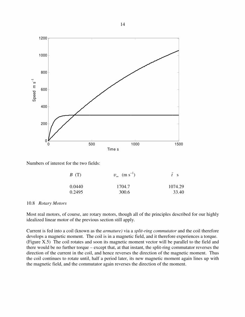
Integration of equation 10.12.2 results in the following equation for the growth of the current with

time:

( ).1 )/( tLRe

R

EI

−−= 10.12.3

Thus the current asymptotically approaches its ultimate value of E/R, reaching 63% (i.e. 1 1− −e ) of

its ultimate value in a time L/R. In figure X.10, the current is shown in units of E/R, and the time in

units of L/R. You should check that L/R, which is called the time constant of the circuit, has the

dimensions of time.

21

0 0.5 1 1.5 2 2.50

0.1

0.2

0.3

0.4

0.5

0.6

0.7

0.8

0.9

1

Time

Curr

ent

FIGURE X.10

Here is a problem that will give practice in sending a current through an inductor, applying

Kirchhoff’s rules, and solving differential equations. There is a similar problem involving a

capacitor, in Chapter 5, Section 5.19.

In the above circuit, while the switch is open, )2/(21 REII == and 03 =I . Long after the switch

is closed and steady currents have been reached, I1 will be )3/(2 RE , and I2 and I3 will each be

)3/( RE . But we want to investigate what happens in the brief moment while the current is

changing.

We apply Kirchhoff’s rules:

RIRIE 21 += 10.12.4

L E

R R

R

I1 I3

I2

22

0233 =−+ RIILRI & 10.12.5

321 III += , 10.12.6

[Getting the sign of 3IL & right in equation 10.12.5 is important. Think of the inductor as a battery of

EMF 3IL & oriented like this: .]

Eliminate I1 and I2 to get a single equation in I3.

L

EI

L

R

dt

dI

22

33

3 =+ . 10.12.7

This is of the form baydx

dy=+ , and those experienced with differential equations will have no

difficulty in arriving at the solution

L

Rt

AeR

EI 2

3

33

−

+= 10.12.8

With the initial condition that I3 = 0 when t = 0, this becomes

−=

−L

Rt

eR

EI 2

3

3 13

10.12.9

The other currents are found from Kirchhoff’s rules (equations 10.12.4-6). I make them:

+=

−L

Rt

eR

EI 2

3

21

2 13

10.12.10

−=

−L

Rt

eR

EI 2

3

21

1 23

10.12.11

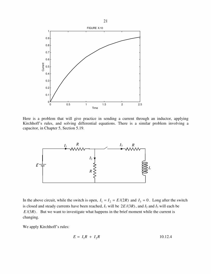
Thus I1 goes from initially R

E

2to finally .

3

2

R

E

I2 goes from initially R

E

2 to finally .

3R

E

I3 goes from initially zero to finally .3R

E

Here are graphs of the currents (in units of E/R) as a function of time (in units of )3/(2 RL ).

23

0 0.5 1 1.5 2 2.5 30

0.1

0.2

0.3

0.4

0.5

0.6

0.7

t

I1

I2

I3

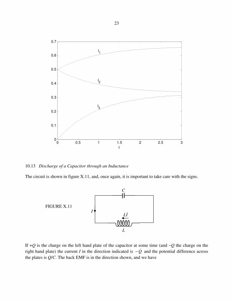
10.13 Discharge of a Capacitor through an Inductance

The circuit is shown in figure X.11, and, once again, it is important to take care with the signs.

If +Q is the charge on the left hand plate of the capacitor at some time (and −Q the charge on the

right hand plate) the current I in the direction indicated is Q&− and the potential difference across

the plates is Q/C. The back EMF is in the direction shown, and we have

C

FIGURE X.11

L

IL & I

24

,0=− ILC

Q& 10.13.1

or .0=+ QLC

Q&& 10.13.2

This can be written ,LC

QQ −=&& 10.13.3

which is simple harmonic motion of period 2π LC . (verify that this has dimensions of time.)

Thus energy sloshes to and fro between storage as charge in the capacitor and storage as current in

the inductor.

If there is resistance in the circuit, the oscillatory motion will be damped, the charge and current

eventually approaching zero. But, even if there is no resistance, the oscillation does not continue

for ever. While the details are beyond the scope of this chapter, being more readily dealt with in a

discussion of electromagnetic radiation, the periodic changes in the charge in the capacitor and the

current in the inductor, result in an oscillating electromagnetic field around the circuit, and in the

generation of an electromagnetic wave, which carries energy away at a speed of 1 0 0/ ( ) .µ ε

Verify that this has the dimensions of speed, and that it has the value 2.998 % 108 m s

−1. The

motion in the circuit is damped just as if there were a resistance of )/(1/ 0000 ε=µ=εµ cc in the

circuit. Verify that this has the dimensions of resistance and that it has a value of 376.7 Ω. This

effective resistance is called the impedance of free space.

10.14 Discharge of a Capacitor through an Inductance and a Resistance

In the section and the next, the reader is assumed to have some experience in the solution of

differential equations. When we arrive at a differential equation, I shall not go into the mechanics

of how to solve it, I shall merely write down the solution of the equation immediately following it,

without explanation. It is not assumed that a reader will immediately be able to solve the equation

is his or her head, but would be able to do so given half an hour in a quiet room. Those with no

experience in differential equations will have to take the solutions given on trust.

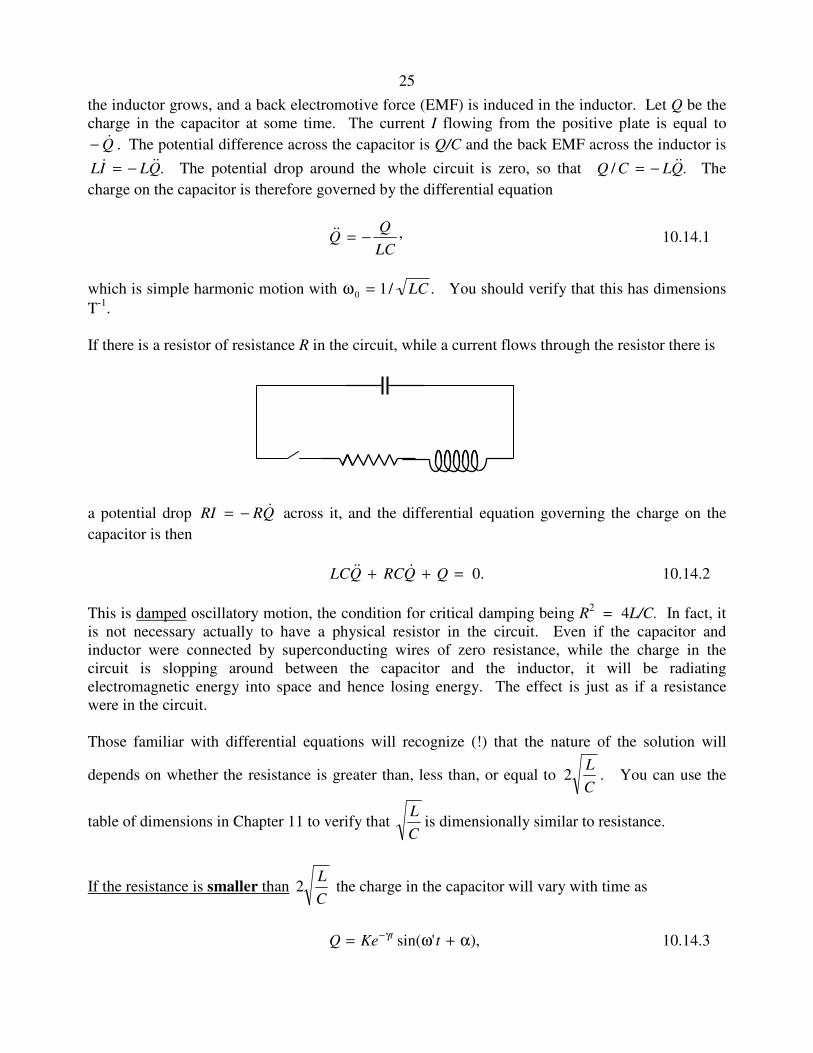
A charged capacitor of capacitance C is connected in series with a switch and an inductor of

inductance L. The switch is closed, and charge flows out of the capacitor and hence a current flows

through the inductor. Thus while the electric field in the capacitor diminishes, the magnetic field in

25

the inductor grows, and a back electromotive force (EMF) is induced in the inductor. Let Q be the

charge in the capacitor at some time. The current I flowing from the positive plate is equal to

Q&− . The potential difference across the capacitor is Q/C and the back EMF across the inductor is

.QLIL &&& −= The potential drop around the whole circuit is zero, so that ./ QLCQ &&−= The

charge on the capacitor is therefore governed by the differential equation

,LC

QQ −=&& 10.14.1

which is simple harmonic motion with ω0 1= / .LC You should verify that this has dimensions

T-1

.

If there is a resistor of resistance R in the circuit, while a current flows through the resistor there is

a potential drop QRRI &−= across it, and the differential equation governing the charge on the

capacitor is then

.0=++ QQRCQLC &&& 10.14.2

This is damped oscillatory motion, the condition for critical damping being R2 = 4L/C. In fact, it

is not necessary actually to have a physical resistor in the circuit. Even if the capacitor and

inductor were connected by superconducting wires of zero resistance, while the charge in the

circuit is slopping around between the capacitor and the inductor, it will be radiating

electromagnetic energy into space and hence losing energy. The effect is just as if a resistance

were in the circuit.

Those familiar with differential equations will recognize (!) that the nature of the solution will

depends on whether the resistance is greater than, less than, or equal to C

L2 . You can use the

table of dimensions in Chapter 11 to verify that C

Lis dimensionally similar to resistance.

If the resistance is smaller than C

L2 the charge in the capacitor will vary with time as

),'sin( α+ω= γ− tKeQ t 10.14.3

26

where ,4

1',/

2

2

L

R

LCLR −=ω=γ 10.14.4

and K and α are arbitrary constants of integration, which depend upon the initial conditions. If the

initial conditions are such that, at time 0, 0QQ = and ,0== IQ& the equation becomes

.'sin0 teQQt ω= γ− 10.14.5

This is a sine function whose amplitude decreases exponentially with time.

If the resistance is larger than C

L2 the charge in the capacitor will vary with time as

,21 ttBeAeQ

λ−λ− += 10.14.6

where LCL

R

L

R

LCL

R

L

R 1

42,

1

42 2

2

22

2

1 −+=λ−−=λ 10.14.7

Here, and A and B are arbitrary constants of integration, which depend upon the initial conditions.

If the initial conditions are such that, at time 0, 0QQ = and ,0== IQ& the equation becomes

( ).21

12

12

0 ttee

QQ

λ−λ− λ−λλ−λ

= 10.14.8

Thus, with these initial conditions, Q decreases monotonically, without oscillation, to zero as .∞→t

If the resistance is equal to C

L2 the charge in the capacitor will vary with time as

).1(2 atKeQ L

Rt

+=−

10.14.9

If the initial conditions are such that, at time 0, 0QQ = and ,0== IQ& the equation becomes

+=

−

L

RteQQ L

Rt

212

0 , 10.14.10

which decreases monotonically to zero as ,∞→t reaching 021 Q at ./3567.3 LRt =

27

10.15 Charging a Capacitor through a Resistor and an Inductor

In Chapter 5 Section 5.19 we connected a battery to a capacitance and a resistance in series to see

how the current in the circuit and the charge in the capacitor varied with time; In this chapter,

Chapter 10 Section 10.12, we connected a battery to an inductance and a resistance in series to see

how the current increased with time. We have not yet connected a battery to R, C and L in series.

We are about to do this. We also recall, from Chapter 5 Section 5.19, when we connect a battery to

C and R in series, the current apparently increases instantaneously from zero to E/R as soon as we

closed the switch. We pointed out that any real circuit (which is necessarily a loop) must have

some inductance, however small, and consequently the current takes a finite time, however small,

to reach its maximum value after the switch is closed.

The differential equation that shows how the EMF of the battery is equal to the sum of the potential

differences across the three elements is

ILCQIRE &++= / 10.15.1

If we write QI &= and QI &&& = we arrive at the differential equation for the charge in the capacitor:

ECQQRCQLC =++ &&& 10.15.2

The general solutions to this are the same as for equation 10.14.2 except for the addition of the

particular integral, which devotees of differential equations will recognize as simply EC. The

general solutions for the current I can be found by differentiating the solutions for Q with respect to

time.

Thus the general solutions are

If the resistance is smaller than C

L2 the charge in the capacitor and the current in the circuit will

vary with time as

.)'sin( ECtKeQ t +α+ω= γ− 10.15.3

)].'sin()'cos('[ α+ωγ−α+ωω= γ− ttKeI t 10.15.4

The definitions of the constants γ and 'ω were given by equations 10.14.4.

If the resistance is larger than C

L2 the charge in the capacitor and the current in the circuit will

vary with time as

.21 ECBeAeQtt ++= λ−λ− 10.15.5

).( 21

21tt

BeAeIλ−λ− λ+λ−= 10.15.6

The definitions of the constants λ1 and λ2 were given by equations 10.14.7

28

If the resistance is equal to C

L2 the charge in the capacitor and the current in the circuit will

vary with time as

.)1(2 ECatKeQ L

Rt

++=−

10.15.7

.)1(2

2

−−=

−

atL

RaKeI L

Rt

10.15.8

The constants of integration can be found from the initial conditions. At t = 0, Q, the charge in the

capacitor, is zero. (This is different from the example in Section 10.14, where the initial charge

was Q0. Also at t = 0, the current I = 0. Indeed this is one of the motivations for doing this

investigation - remember our difficulty in Section 5.19. The results of applying the initial

conditions are:

If the resistance is larger than C

L2 the constants of integration are given by

γ

ω=α

'tan 10.15.9

and α

−=sin

ECK 10.15.10

These could in principle be inserted into equations 10.15.3 and 10.15.4. For computational

purposes it is easier to leave the equations as they are.

If the resistance is larger than C

L2 the charge in the capacitor and the current in the circuit will

vary with time as

λ−λ

λ−λ−=

λ−λ−

12

1221

1tt

eeECQ 10.15.11

( ).21

12

21 tteeECI

λ−λ− −

λ−λ

λλ= 10.15.12

If the resistance is equal to C

L2 the charge in the capacitor and the current in the circuit will

vary with time as

+−= −

L

RteECQ

LRt

211 )2/( 10.15.13

.4

)2/(

2

2LRt

teL

ECRI

−= 10.15.14

29

It will be noted, in all three cases, that the complementary function of the solution to the differential

equation is a transient which eventually disappears, while the particular integral represents the

final steady state solution. Readers may have noticed that, when a fuse blows, it often blows just

when you switch on; it is the transient surge that strikes the fatal blow.

The situation that initially interested us in this problem was the case when the inductance in the

circuit was very small - that is, when the resistance is larger than C

L2 . We were concerned that,

when the inductance was actually zero, the current apparently

immediately rose to EC as soon as the switch was closed. So let us look at equation 10.15.12. If we

multiply both sides by CR it can then be written in dimensionless form as

( )τ−τ− −

−= 21

12

21

/

llee

ll

ll

RE

I, 10.15.15

where )/(CRt=τ and ii CRl λ= . 10.15.16

In other words we are expressing time in units of CR.

It can be observed, by differentiation of equation 10.15.15, that the current will reach a maximum

value (which is less than E/R) at time given by

.)/ln()/ln(

12

12

12

12

λ−λ

λλ=

−=τ

ll

ll 10.15.18

The two λ constants, first defined in equations 10.14.7, can be written in the form

−+=λ

−−=λ

RC

RL

L

R

RC

RL

L

R )/(411

2,

)/(411

221 10.15.19

I introduce the dimensionless ratio

CR

RLx

/= , 10.15.20

so that

x

xl

x

xl

2

411,

2

41121

−+=

−−= 10.15.21

In the table and graph below I show how the current I changes with time (equation 10.15.12, or, in

dimensionless form, 10.15.15) for101=x and for

251=x . The current is given in units of E/R , and

the time is in units of RC. Only if the inductance of the circuit is exactly zero (which cannot

30

possibly be obtained in any real closed circuit) will the current jump immediately from 0 to E/R at

the instant when the switch is closed.

x l1 l1 12

21

ll

ll

− τmax

RE

I

/

max

0.10 1.12702 8.87298 1.29099 0.26639 0.83473

0.04 1.04356 23.95644 1.09109 0.13676 0.90476

0 0.1 0.2 0.3 0.4 0.5 0.6 0.7 0.8 0.9 10

0.1

0.2

0.3

0.4

0.5

0.6

0.7

0.8

0.9

1

time

cu

rre

nt

x = 0.10

x = 0.04

31

10.16 Energy Stored in an Inductor

During the growth of the current in an inductor, at a time when the current is i and the rate of

increase of current is i&, there will be a back EMF .iL& The rate of doing work against this back

EMF is then .iLi& The work done in time dt is ,diLidtiLi =& where di is the increase in current in

time dt. The total work done when the current is increased from 0 to I is

,2

21

0LIdiiL

I

=∫ 10.16.1

and this is the energy stored in the inductance. (Verify the dimensions.)

10.17 Energy Stored in a Magnetic Field

Recall your derivation (Section 10.11) that the inductance of a long solenoid is µn Al2 . The energy

stored in it, then, is 12

2 2µn AlI . The volume of the solenoid is Al, and the magnetic field is

B n I H n I= =µ , .or Thus we find that the energy stored per unit volume in a magnetic field is

B

BH H2

12

12

2

2µµ= = . 10.17.1

In a vacuum, the energy stored per unit volume in a magnetic field is 12 0

2µ H - even though the

vacuum is absolutely empty!

Equation 10.16.2 is valid in any isotropic medium, including a vacuum. In an anisotropic medium,

B and H are not in general parallel – unless they are both parallel to a crystallographic axis. More

generally, in an anisotropic medium, the energy per unit volume is 12

B H• .

Verify that the product of B and H has the dimensions of energy per unit volume.