chapter 11. angular momentum: general theory

11. Angular Momentum Theory, November 20, 2009 1

Chapter 11. Angular Momentum: General Theory

§ 1 Introduction. Angular momentum is intimately related to rotationalmotion of a system of particles. It is essential for understanding the infraredand microwave spectra of a molecule and the properties of the electrons inatoms.The spin of an electron or of a nucleus is an angular momentum that has

no classical analog. The spin is accompanied by magnetic moment, whichmeans that we can change the energy of a particle by acting on it with anexternal magnetic field. NMR and ESR spectroscopies are based on thisability. Understanding these extremely rich and important spectroscopictechniques requires a good understanding of angular momentum.In this chapter we define the dynamics of angular momentum through

the commutation relations between the operators representing its projectionon the coordinate axes. These commutation relations allow us to determinethe eigenstates of the angular momentum operator and derive the matrixrepresentation of the relevant operators. The chapters that follow use thistheory to examine the properties of spin, the orbital angular momentum, andthe angular momentum of more than one particle.

§ 2 The definition of the angular momentum operator. In quantum me-chanics, we encounter two kinds of angular momenta. The orbital angularmomentum is very similar to the angular momentum in classical mechanics.It describes some aspects of the motion of a particle and it is defined by

L = r × p (1)

where r is the position of a particle and p is its momentum. To define the

operatorˆL describing the orbital angular momentum in quantum mechanics,

we replace, in Eq. 1, r with r and p with p:

ˆL = r × p (2)

In addition to the orbital angular momentum, the particles studied inquantum mechanics have an intrinsic angular momentum called spin. Thisis not caused by the motion of the particle (e.g. its rotation); it is insteada property similar to charge or mass. This angular momentum cannot be


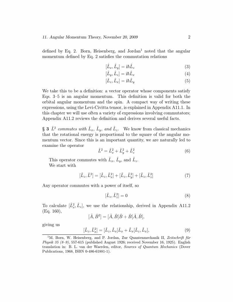
defined by Eq. 2. Born, Heisenberg, and Jordan1 noted that the angularmomentum defined by Eq. 2 satisfies the commutation relations

[Lx, Ly] = ihLz (3)

[Ly, Lz] = ihLx (4)

[Lz, Lx] = ihLy (5)

We take this to be a definition: a vector operator whose components satisfyEqs. 3—5 is an angular momentum. This definition is valid for both theorbital angular momentum and the spin. A compact way of writing theseexpressions, using the Levi-Civitta tensor, is explained in Appendix A11.1. Inthis chapter we will use often a variety of expressions involving commutators;Appendix A11.2 reviews the definition and derives several useful facts.

§ 3 L2 commutes with Lx, Ly, and Lz. We know from classical mechanicsthat the rotational energy is proportional to the square of the angular mo-mentum vector. Since this is an important quantity, we are naturally led toexamine the operator

L2 = L2x + L2y + L

2z (6)

This operator commutes with Lx, Ly, and Lz.We start with

[Lz, L2] = [Lz, L

2x] + [Lz, L

2y] + [Lz, L

2z] (7)

Any operator commutes with a power of itself, so

[Lz, L2z] = 0 (8)

To calculate [L2x, Lz], we use the relationship, derived in Appendix A11.2(Eq. 160),

[A, B2] = [A, B]B + B[A, B],

giving us[Lz, L

2x] = [Lz, Lx]Lx + Lx[Lz, Lx], (9)

1M. Born, W. Heisenberg, and P. Jordan, Zur Quantenmechanik II, Zeitschrift furPhysik 35 (8—9), 557-615 (published August 1926; received November 16, 1925). Englishtranslation in: B. L. van der Waerden, editor, Sources of Quantum Mechanics (DoverPublications, 1968, ISBN 0-486-61881-1).


followed by Eq. 5, to obtain

[Lz, L2x] = ihLyLx + ihLxLy = ih LyLx + LxLy (10)

You can show similarly that

[Lz, L2y] = −ih LyLx + LxLy (11)

Using Eqs. 8—11 in Eq. 7 gives

[L2, Lz] = 0 (12)

In the same way, you can show that

[L2, Lx] = 0 (13)

and[L2, Ly] = 0 (14)

Common sense tells us that if Eq. 12 is true, then Eqs. 13 and 14 must alsobe true, because there is no physical agent that differentiates between theOZ and OX or OY directions.

§ 4 The eigenstates of L2 and Lz. Since L2 commutes with Lz, there existsa set of eigenfunctions of L2 that are also eigenfunctions of Lz. Because Lzdoes not commute with Lx or with Ly, a joint eigenstate of L

2 and Lz cannot

be an eigenstate of Ly or of Lz.

Let us examine in more detail what this means. Since L2 and Lz commute,there exists a set of kets |Lz;α, β that satisfy the eigenvalue equations forthose two operators:

L2|Lz;α,β = α|Lz;α,β (15)

Lz|Lz;α,β = β|Lz;α, β (16)

α is the value that L2 can have in a measurement. It is therefore relatedto the rotational energy. β is the value that the projection of the angularmomentum on the Z-axis can take. The symbol Lz inside the ket reminds usthat this is an eigenket of Lz, not of Lx or Ly.

But L2 also commutes with Lx, so there must exist a set of kets |Lx;α, βsuch that

L2|Lx;α,β = α|Lx;α,β (17)

Lx|Lx;α,β = β|Lx;α,β (18)


As long as no electric or magnetic field acts on the system there is no physicaldifference between the OX and the OZ axes. Therefore, the values that βcan take in |Lx;α, β are the same as the values it can take in |Lz;α,β .In what follows, we concentrate on the joint eigenstates of L2 and Lz. At

this point there is no reason to prefer Lz over Lx or Ly.Suppose that we have performed an experiment that places the system

in the state |Lz;α,β . We can measure L2 and get the value α, or we canmeasure Lz and get the value β. However, if we measure Lx, when the systemis in state |Lz;α,β , we find Lx to be β with the probability

| Lx;α, β |Lz;α, β |2

When the system is in the state |Lz;α, β , we know L2 and Lz with certaintybut we only know the probability that Lx takes a given value. For someonefamiliar with quantum mechanics, this is not surprising. Lz and Lx do notcommute so the eigenstate |Lz;α,β cannot be an eigenstate of Lx.These results are incomprehensible within classical physics, where there

is no physical law to prevent us from knowing with certainty all three pro-jections of any vector once we know the state of the system (i.e. the valuesof the position and of the momentum).

§ 5 L2 and Lz commute with other operators. One difficulty in graspingthe physics of angular momentum comes from the fact that in many con-crete problems, Lx, Ly, and Lz are not the only operators describing thesystem. For example, we might examine two particles interacting through acentral force. This means that the potential energy V (r) depends only onthe distance r between the particles and is independent of their orientationin space. You know two examples of such systems: the hydrogen atom andthe diatomic molecule.The eigenvalue problem for the Hamiltonian of the hydrogen atom is (see

Metiu, Quantum Mechanics, p. 206)

− h2

2μ

1

r2∂

∂rr2∂ψ

∂r+

L2

2μr2ψ + V (r)ψ = Eψ (19)

We see that besides the angular momentum squared L2, the equation con-tains the potential energy V (r) and the radial kinetic energy (the first term).You have also learned that the Hamiltonian H of the hydrogen atom com-mutes with L2 and with Lz. This means that H, L

2, and Lz have common


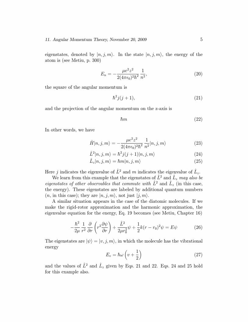
eigenstates, denoted by |n, j,m . In the state |n, j,m , the energy of theatom is (see Metiu, p. 300)

En = − μe2z2

2(4π 0)2h2

1

n2, (20)

the square of the angular momentum is

h2j(j + 1), (21)

and the projection of the angular momentum on the z-axis is

hm (22)

In other words, we have

H|n, j,m = − μe2z2

2(4π 0)2h2

1

n2|n, j,m (23)

L2|n, j,m = h2j(j + 1)|n, j,m (24)

Lz|n, j,m = hm|n, j,m (25)

Here j indicates the eigenvalue of L2 and m indicates the eigenvalue of Lz.We learn from this example that the eigenstates of L2 and Lz may also be

eigenstates of other observables that commute with L2 and Lz (in this case,the energy). These eigenstates are labeled by additional quantum numbers(n, in this case); they are |n, j,m , not just |j,m .A similar situation appears in the case of the diatomic molecules. If we

make the rigid-rotor approximation and the harmonic approximation, theeigenvalue equation for the energy, Eq. 19 becomes (see Metiu, Chapter 16)

− h2

2μ

1

r2∂

∂rr2∂ψ

∂r+

L2

2μr20ψ +

1

2k(r − r0)2ψ = Eψ (26)

The eigenstates are |ψ = |v, j,m , in which the molecule has the vibrationalenergy

Ev = hω v +1

2(27)

and the values of L2 and Lz given by Eqs. 21 and 22. Eqs. 24 and 25 holdfor this example also.


In general, when L2 and Lz commute with other operators, their eigen-states must be eigenstates of those operators. When we need to make thisexplicit, these eigenstates will be labeled |a, j,m , where a tells us the valuethat the quantities represented by these other operators takes, when thesystem is in a pure state |a, j,m and a measurement is made.

§ 6 A more convenient notation. I now change notation by writing

α = h2j(j + 1) (28)

β = hm (29)

|Lz;α,β = |Lz; j,m (30)

The eigenvalue equations Eqs. 15 and 16 become

L2|Lz; j,m = h2j(j + 1)|Lz; j,m (31)

andLz|Lz; j,m = hm|Lz; j,m (32)

Setting α = h2j(j + 1) needs further examination. We must have

α ≥ 0 (33)

because α is a value that L2 can take. It is a minor complication that theequation α = h2j(j + 1) has two solutions for j:

j1 = −121 + 1 + 4α/h2 (34)

and

j2 =1

2−1 + 1 + 4α/h2 (35)

Because α/h2 ≥ 0, both roots j1 and j2 are real, j1 is negative, and j2 is non-negative. Remember that α is a physical observable while j is an arbitrarymathematical quantity introduced for convenience. You can verify that thenegative values of j give the same values of α as the non-negative ones. Wecan choose either for indexing the kets, and we choose

j ≥ 0 (36)

Note also that m must be a real number (hm is a value of Lz). BecauseLz is equally likely to be positive or negative, we expect m to be able to take


both positive and negative values. Moreover, we guess that if m is an allowedvalue, then −m is also allowed since the projection of the angular momentumvector on the OZ axis can be oriented along OZ (m > 0) or opposite to it(m < 0).

§ 7 A summary of our task. To set up the theory of angular momentum,we need to do the following.

1. Since most calculations in quantum mechanics are done by representingoperators by matrices, we need to use the kets |Lz; j,m as a basis setand find out how to calculate the matrix elements Lz; j,m | O |Lz; j ,mfor O = Lx and Ly.

2. Find the values of j andm allowed by the eigenvalue equations Eqs. 31—32.

To reach these objectives, we only have the commutation relations Eqs. 3—5 and our wits. The strategy is simple but tedious. We know how L2 andLz act on |Lz; j,m . Therefore we must use the commutation relations toexpress Lx and Ly in terms of L

2 and Lz. Determining the allowed values ofj and m is more subtle and cannot be reduced to a few sentences.

§ 8 The ladder operators. In vector calculus, one often describes a vectorvx, vy, vz through its spherical components vx+ivy, vx− ivy, vz. It mighttherefore be useful to take a look at the operators

L+ ≡ Lx + iLy (37)

andL− ≡ Lx − iLy (38)

along with Lz and L2. If we find out how L+ and L− act on |Lz; j,m , then

it is easy to use

Lx =L+ + L−

2(39)

and

Ly =L+ − L−2i

(40)

to find out how Lx and Ly act on |Lz; j,m . Working with L+ and L− willprove to be fruitful.


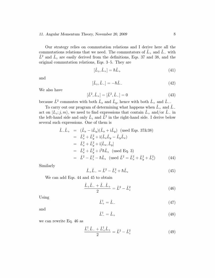
Our strategy relies on commutation relations and I derive here all thecommutations relations that we need. The commutators of L+ and L− withL2 and Lz are easily derived from the definitions, Eqs. 37 and 38, and theoriginal commutation relations, Eqs. 3—5. They are

[Lz, L+] = hL+ (41)

and[Lz, L−] = −hL− (42)

We also have[L2, L+] = [L

2, L−] = 0 (43)

because L2 commutes with both Lx and Ly, hence with both L+ and L−.To carry out our program of determining what happens when L+ and L−

act on |Lz; j,m , we need to find expressions that contain L+ and/or L− inthe left-hand side and only Lz and L

2 in the right-hand side. I derive belowseveral such expressions. One of them is

L−L+ = (Lx − iLy)(Lx + iLy) (used Eqs. 37&38)= L2x + L

2y + i(LxLy − LyLx)

= L2x + L2y + i[Lx, Ly]

= L2x + L2y + i

2hLz (used Eq. 3)

= L2 − L2z − hLz (used L2 = L2x + L2y + L2z) (44)

SimilarlyL+L− = L2 − L2z + hLz (45)

We can add Eqs. 44 and 45 to obtain

L+L− + L−L+2

= L2 − L2z (46)

UsingL†+ = L− (47)

andL†− = L+ (48)

we can rewrite Eq. 46 as

L†−L− + L†+L+

2= L2 − L2z (49)


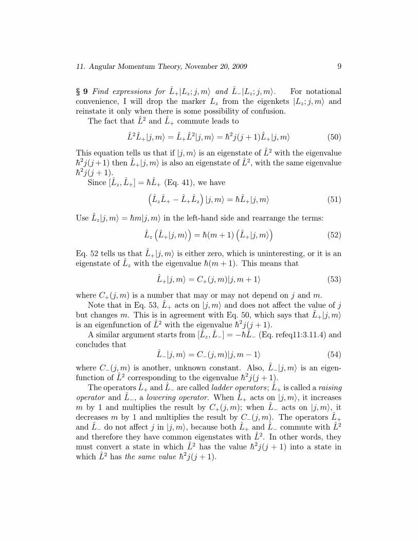
§ 9 Find expressions for L+|Lz; j,m and L−|Lz; j,m . For notationalconvenience, I will drop the marker Lz from the eigenkets |Lz; j,m andreinstate it only when there is some possibility of confusion.The fact that L2 and L+ commute leads to

L2L+|j,m = L+L2|j,m = h2j(j + 1)L+|j,m (50)

This equation tells us that if |j,m is an eigenstate of L2 with the eigenvalueh2j(j+1) then L+|j,m is also an eigenstate of L2, with the same eigenvalueh2j(j + 1).Since [Lz, L+] = hL+ (Eq. 41), we have

LzL+ − L+Lz |j,m = hL+|j,m (51)

Use Lz|j,m = hm|j,m in the left-hand side and rearrange the terms:

Lz L+|j,m = h(m+ 1) L+|j,m (52)

Eq. 52 tells us that L+|j,m is either zero, which is uninteresting, or it is aneigenstate of Lz with the eigenvalue h(m+ 1). This means that

L+|j,m = C+(j,m)|j,m+ 1 (53)

where C+(j,m) is a number that may or may not depend on j and m.Note that in Eq. 53, L+ acts on |j,m and does not affect the value of j

but changes m. This is in agreement with Eq. 50, which says that L+|j,mis an eigenfunction of L2 with the eigenvalue h2j(j + 1).A similar argument starts from [Lz, L−] = −hL− (Eq. refeq11:3.11.4) and

concludes thatL−|j,m = C−(j,m)|j,m− 1 (54)

where C−(j,m) is another, unknown constant. Also, L−|j,m is an eigen-function of L2 corresponding to the eigenvalue h2j(j + 1).The operators L+ and L− are called ladder operators ; L+ is called a raising

operator and L−, a lowering operator. When L+ acts on |j,m , it increasesm by 1 and multiplies the result by C+(j,m); when L− acts on |j,m , itdecreases m by 1 and multiplies the result by C−(j,m). The operators L+and L− do not affect j in |j,m , because both L+ and L− commute with L2

and therefore they have common eigenstates with L2. In other words, theymust convert a state in which L2 has the value h2j(j + 1) into a state inwhich L2 has the same value h2j(j + 1).


This expresses L+L− in terms of L2 and Lz. I know how L2 and Lz act on|j,m and therefore I can readily calculate the matrix element in Eq. 63.Eq. 63 determines the absolute value of C+ but not its phase. Since all

physical properties of a ket are independent of a phase factor in front of it,I can take in C+ any phase I want. I choose it so that

C+(j,m) = j,m | L†+L+ | j,m (64)

Now use Eq. 44 in Eq. 64:

C+(j,m) = j,m | L2 − L2z − hLz | j,m (65)

Using the eigenvalue equations for L2 and Lz (Eqs. 31—32), we rewrite Eq. 65as

C+(j,m) = h j(j + 1)−m(m+ 1) (66)

(we used j,m | j,m = 1).Finally, putting C+(j,m) given by Eq. 66 into Eq. 53 gives

L+|j,m = h j(j + 1)−m(m+ 1) |j,m+ 1 (67)

Note that L+|j,m is an eigenstate of L2 corresponding to the eigenvaluehj(j + 1) and an eigenstate of Lz corresponding to the eigenvalue (m+ 1)h.However, |j,m is not an eigenstate of L+. It should not be, because L+does not commute with L2 or with Lz.To calculate C−(j,m), we follow the reasoning used to find C+(j,m). This

leads toC−(j,m) = h j(j + 1)−m(m− 1) (68)

andL−|j,m = h j(j + 1)−m(m− 1) |j,m− 1 (69)

We can now calculate (use Eqs. 66, 69, 39)

Lx|j,m =1

2(L+ + L−)|j,m

=1

2[C+(j,m)|j,m+ 1 + C−(j,m)|j,m− 1 ] (70)

Similarly (use Eqs. 66, 69, 40)

Ly|j,m =1

2i[C+(j,m)|j,m+ 1 − C−(j,m)|j,m− 1 ] (71)


§ 11 The matrix elements of L+, L−, Lx, Ly in the basis set |j,m . Now

that we know how L+ and L− act on |j,m (Eqs. 67 and 69), we can calculatethe matrix elements

j ,m | L+ | j,m = h j(j + 1)−m(m+ 1) j ,m | j,m+ 1= h j(j + 1)−m(m+ 1) δj jδm ,m+1 (72)

The only non-zero matrix elements are those for whichm = m+1 and j = j.Therefore only

j,m+ 1 | L+ | j,m = h j(j + 1)−m(m+ 1) (73)

differs from zero.The matrix elements of L− are

j ,m | L− | j,m = h j(j + 1)−m(m− 1) δj jδm ,m−1 (74)

and only

j,m− 1 | L− | j,m = h j(j + 1)−m(m− 1) (75)

differs from zero.Since (see Eq. 39)

Lx =L+ + L−

2

we have

j ,m | Lx | j,m =h

2(C+(j,m) δj jδm ,m+1 + C−(j,m) δj jδm ,m−1) (76)

Only the matrix elements

j,m+ 1 | Lx | j,m =h

2C+(j,m) (77)

and

j,m− 1 | Lx | j,m =h

2C−(j,m) (78)

differ from zero.Using (see Eq. 40)

Ly =L+ − L−2i


with Eqs. 72 and 74 leads to

j ,m | Ly | j,m =h

2i(C+(j,m) δj jδm ,m+1 − C−(j,m) δj jδm ,m−1) (79)

Only the matrix elements

j,m+ 1 | Ly | j,m =h

2iC+(j,m) (80)

and

j,m− 1 | Ly | j,m = − h2iC−(j,m) (81)

differ from zero.This covers all the matrix elements used in applications. However, we

still don’t know what values j and m can take, since we do not know theeigenvalues of L2 and Lz. Next, we start working to find them.

The values of j and mWe have decided to use the eigenstates |j,m of L2 and Lz as a basis set

for other operators relevant to angular momentum, and we have managedto calculate their matrix elements. The remaining task is to determine theallowed values of j and m.

§ 12 For a given j, m has a highest and a lowest value. A classical inter-pretation of angular momentum tells us that if L2 is fixed then Lz must havean upper and a lower bound. Indeed the projection of a vector on an axiscan at most be equal to the length of the vector: the projection has theupper bound and the lower bound − . Since quantum mechanics is notclassical mechanics, it will be reassuring to prove that, for a given j, m hasan upper and a lower bound.Recall that (Eqs. 46 and 49)

L+L− + L−L+2

= L2 − L2z (82)

andL†−L− + L

†+L+

2= L2 − L2z (83)


From properties of the inner product, we know that for any ket |x andany operator A, we have x | A†A | x ≥ 0 (with equality only when A|x = 0).Taking the matrix element of the operator in Eq. 83 with the non-zero ket|j,m gives

j,m | L†−L− | j,m + j,m | L†+L+ | j,m = 2h2(j(j + 1)−m2) (84)

Since the left-hand side cannot be negative, we conclude that

j(j + 1)−m2 ≥ 0 (85)

This means that if j is fixed then m has both a lower bound and an upperbound. We don’t know what the bounds are but we know that they exist, solet us denote them by m and mu.This gives us two new equations to play with:

L+|j,mu = 0 (86)

L−|j,m = 0 (87)

To derive them, observe that, according to Eq. 53, L+|j,mu = C+(j,mu)|j,mu+1 . Since no value of m can be larger than mu, the state |j,mu + 1 can-not exist and the ket is zero (which proves Eq. 86). One arrives at Eq. 87similarly.Now let us act with L− on Eq. 86 and with L+ on Eq. 87, to obtain

L−L+|j,mu = 0 (88)

L+L−|j,m = 0 (89)

Why do I do that? Because we know that (Eq. 44)

L−L+ = L2 − L2z − hLz;the right-hand side of this equation contains only operators that act on |j,maccording to known rules, which means that we can calculate

0 = L−L+|j,m = (L2 − L2z − hLz)|j,m= (h2j(j + 1)− h2m2

u − h2mu)|j,mu (90)

This implies thatj(j + 1)−m2

u −mu = 0 (91)


Similarly, using (see Eq. 45)

L+L− = L2 − L2z + hLzin Eq. 89 gives

j(j + 1)−m2 +m = 0 (92)

Solving Eq. 92 for j(j + 1) and using the result in Eq. 91 gives

mu(mu + 1) = m (m − 1) (93)

This equation has two solutions

mu = −m (94)

andmu = m − 1 (95)

The second root is excluded by the fact that mu ≥ m by definition.We see therefore that mu = −m . Symmetry requires the possible pro-

jections of L along OZ to be equal to and of opposite sign to the possibleprojections in the direction opposite to OZ. Eq. 94 agrees with this require-ment.

§ 13 The values of m and j. We have learned a lot but we still don’t knowwhich values j and m can take. Here we settle this question.Let us consider a ket |j,m0 where m0 is an allowed value of m for the

given j. Acting on that ket with L+ repeatedly, we obtainL+|j,m0 = C+(j,m0)|j,m0 + 1 ,L2+|j,m0 = C+(j,m0)C+(j,m0 + 1)|j,m0 + 2 ,etc. After some number nu of steps, this procedure must generate a ketproportional to |j,mu . If it did not, then we could apply L+ indefinitely,which contradicts the fact that m has a largest value, namely mu. Thereforewe must have

mu = m0 + nu (96)

where nu is a non-negative integer. Similarly, applying L− to |j,m0 some ntimes produces a ket proportional to |j,m , so that

m = m0 − n (97)


with n a non-negative integer. From Eqs. 96 and 97, it follows that

mu −m = (m0 + nu)− (m0 − n ) = nu + n ≡ n (98)

where n is a non-negative integer. Since we already know that mu = −m(Eq. 94), we conclude that

2mu = n (99)

We also know that (see Eq. 91)

j(j + 1) = m2u +mu = mu(mu + 1) (100)

This has two solutionsj = mu (101)

andj = −mu − 1 (102)

Eq. 102 is not compatible with the facts that mu ≥ 0 and j ≥ 0, so we caneliminate it as irrelevant.Now combining mu = n/2 (Eq. 99) with Eq. 101 gives

j =n

2(103)

We have obtained a startling result: j can be either a non-negative integer(if n is even) or a half-integer (if n is odd). In addition, the largest value ofm is j and (since m = −mu) the smallest value of m is −j. Therefore mcan take the 2j + 1 values −j, −j + 1,. . . , j − 1, j.The theory of orbital angular momentum (see Metiu, Chapter 14, p. 220ff),

based on the equation L = r× p, tells us that half-integer values of j are notallowed for orbital angular momentum. However, by using the commutationrelations to define the angular momentum, we have found that j can be ei-ther integer or half-integer. We know of no additional condition that we canuse to conclude that half-integers are not allowed in general. Therefore thepostulate that the electron has an intrinsic angular momentum (the spin)with j = 1/2 is in harmony with conclusions derived from the commutationrelations.

§ 14 Summary. This lengthy derivation led us to the following results. L2and Lz have common eigenstates |Lz; j,m for which

L2|Lz; j,m = h2j(j + 1) |Lz; j,m (104)


andLz|Lz; j,m = hm |Lz; j,m . (105)

j can be either a non-negative integer or a positive half-integer (that is, ofthe form integer/2). m can take 2j + 1 discrete values

m = −j,−j + 1,−j + 2, . . . , j − 2, j − 1, j (106)

For example, if j = 32then m can take 2× 3

2+ 1 = 4 values, namely

m = −32, −3

2+ 1,

3

2− 1, 3

2= −3

2, −1

2,1

2,3

2

If j = 3 then m takes the 2× 3 + 1 = 7 values −3,−2, 1, 0, 1, 2, 3.We have also found that

Lx|Lz; j,m =1

2[C+(j,m)|Lz; j,m+ 1 + C−(j,m)|Lz; j,m− 1 ] (107)

and

Ly|Lz; j,m =1

2i[C+(j,m)|Lz; j,m+ 1 − C−(j,m)|Lz; j,m− 1 ] (108)

withC+(j,m) = h j(j + 1)−m(m+ 1) (109)

andC−(j,m) = h j(j + 1)−m(m− 1). (110)

Note that |j,m = 0 if m ∈ [−j, j].The matrix elements needed in computations are

Lz; j ,m | Lz | Lz; j,m = δjj δmm hm (111)

Lz; j ,m | L2 | Lz; j,m = δjj δmm h2j(j + 1) (112)

Lz; j ,m | Lx | Lz; j,m = δjjC+(j,m)δm ,m+1 + C−(j,m)δm ,m−1

2(113)

Lz; j ,m | Ly | Lz; j,m = δjjC+(j,m)δm ,m+1 − C−(j,m)δm ,m−1

2i(114)

Note that all these matrix elements are zero if j = j . This means thatin the basis set |Lz; j,m , the matrices of Lx and Ly consist of smallermatrices strung along the diagonal; there are no non-zero matrix elementsj,m | Oj ,m in which j = j if O = Lx, Ly, L+, or L− or any function ofthem.


The eigenvalue problems for angular momentum operators

§ 15 Introduction. We have seen several times that kets are very useful fortheoretical analysis, but practical calculations often use the representation ofkets by vectors and of operators by matrices. In this section I review brieflythe general theory and then apply it to the case of j = 3 as an example.Let us assume that on physical grounds we have decided that a certain

physical system can be described by a ket space generated by the orthonormalbasis set |η1 , |η2 , . . . , |ηN . An arbitrary state |ψ is then represented as

|ψ =N

i=1

|ηi ηi |ψ ≡N

i=1

|ηi ci (115)

and an arbitrary operator O by

O =N

i=1

N

k=1

|ηi ηi | O | ηk ηk| ≡N

i=1

N

k=1

|ηi Oik ηk| (116)

Since we are assumed to know |ηi , i = 1, 2, . . . , N , knowing the vectorψ = c1, c2, . . . , cN (117)

is equivalent to knowing |ψ (because of Eq. 115). Eq. 116 tells us that weknow how to operate with O if we know the matrix elements

Oik ≡ ηi | O | ηk (118)

The basis set kets |ηi are represented by the vectorsη1 = 1, 0, . . . , 0

...ηN = 0, 0, . . . , 1

⎫⎪⎪⎬⎪⎪⎭ (119)

and therefore

ψ =N

i=1

ciηi (120)

The eigenvalue problem O|ψ = o|ψ is represented by the eigenvalue problemfor the matrix O

k

Oikck = o ci,


which in vector-and-matrix notation is written as

Oψ = oψ (121)

or ⎛⎜⎜⎝O11 · · · O1N...

...ON1 · · · ONN

⎞⎟⎟⎠⎛⎜⎜⎝c1...cN

⎞⎟⎟⎠ = o⎛⎜⎜⎝c1...cN

⎞⎟⎟⎠ (122)

The solution of Eq. 122 provides N eigenvectors

ψ(α) ≡ c1(α), . . . , cN(α), α = 1, . . . , N (123)

and N eigenvalues o(1), . . . , o(N).From these we can calculate the N eigenkets |ψ(1) , . . . , |ψ(N) by using

|ψ(α) =N

k=1

ck(α)|ηk , α = 1, 2, . . . , N (124)

§ 16 The matrix-and-vector representation for angular momentum problems.It is natural to use for angular momentum calculations the basis set |j,m .In this basis set, the matrix elements of Lz, L

2, Lx, and Ly are given byEqs. 111—114. When looking at these equations, we notice that all matrixelements in which j = j are zero. The matrices of the operators L2, Lz, Lx,and Ly are therefore block diagonal:⎛⎜⎜⎜⎜⎜⎜⎜⎜⎜⎜⎜⎜⎜⎜⎜⎜⎜⎜⎜⎝

•• • •• • •• • •

• • • • •• • • • •• • • • •• • • • •• • • • •

. . .

⎞⎟⎟⎟⎟⎟⎟⎟⎟⎟⎟⎟⎟⎟⎟⎟⎟⎟⎟⎟⎠All matrix elements other than the dots are zero.We have labeled the rows and the columns in the following order:


• j = 0,m = 0

• j = 1,m = −1• j = 1,m = 0

• j = 1,m = 1

• etc.The state with j = 0 generates a 1× 1 block, the states with j = 1 generatea 3 × 3 block, . . . ; in general, the states having an arbitrary j generate a(2j + 1) × (2j + 1) block. This break-up into blocks makes this basis setparticularly simple to use in calculations. Physically it signifies that stateswith different values of j are not coupled by any of the operators L2, Lz, Lx,and Ly.Because of this “block” property, we can treat physical problems involving

a specific j within a reduced space generated by the basis set

|j,−j , |j,−j + 1 , . . . , |j, j − 1 , |j, j (125)

§ 17 The case j = 1. Let us solve some problems for j = 1. The basis setis

|1,−1 , |1, 0 , |1, 1 (126)

Since we know that j = 1, the first index is superfluous and we use insteadthe notation | − 1 , |0 , |1 . The matrix representing an operator O in thissubspace is

O =

⎛⎜⎜⎝ −1 | O | − 1 −1 | O | 0 −1 | O | 10 | O | − 1 0 | O | 0 0 | O | 11 | O | − 1 1 | O | 0 1 | O | 1

⎞⎟⎟⎠ (127)

A look at Eqs. 111 and 112 tells us that the matrix elements 1,m | L2 | 1,mand 1,m | Lz | 1,m are zero if m = m . Therefore the corresponding matri-ces are diagonal:

L2 = h2(1)(1 + 1)

⎛⎜⎝ 1 0 00 1 00 0 1

⎞⎟⎠ (128)


and

Lz =

⎛⎜⎝ −h 0 00 0 00 0 h

⎞⎟⎠ (129)

No surprise here. The basis set consists of eigenstates |j,m of L2 and Lzand therefore the matrices of these operators, in that basis set, are diagonaland the diagonal elements are the eigenvalues of the operator.The matrices corresponding to Lx and Ly are more interesting. Let us

look at Lx, and use Eq. 113 together with Eqs. 109 and 110. I calculate, asan example, −1 | Lx | − 1 . We have

m = −1 | Lx |m = −1 = 0 (130)

because (see Eq. 113)

δm ,m+1 = δ−1,−1+1 = δ−1,0 = 0

andδm ,m−1 = δ−1,−1−1 = δ−1,−2 = 0

Another example is (use Eq. 113)

m = −1 | Lx |m = 0 =C+(1, 0)δ−1,0+1 + C−(1, 0)δ−1,0−1

2=C−(1, 0)2(131)

withC−(1, 0) = h 1(1 + 1)− 0(0− 1) = h

√2 (132)

Together these give

−1 | Lx | 0 =h√2

(133)

Patiently calculating all the matrix elements leads to2

Lx =

⎛⎜⎜⎝0 h√

20

h√2

0 h√2

0 h√2

0

⎞⎟⎟⎠ (134)

2The top row is m = −1, the middle row is m = 0, and the bottom row is m = 1;the left column is m = −1, the middle column is m = 0, and the right column is m = 1.In all entries j = 1.


These matrix elements were calculated in WorkBook11.Angular Momentum.nb.The matrix must be Hermitian because Lx represents an observable, and

therefore we need only calculate the matrix elements in the lower-left triangle;the ones in the upper-right triangle are then obtained from m | O |m =m | O |m ∗. In addition, the δs in Eq. 113 tell us that the diagonal elements(that is, those with m = m) are zero and that in the lower-left triangle, only0 | Lx | − 1 and 1 | Lx | 0 are nonzero.

Exercise 1 Show that for j = 1

Ly =h√2

⎛⎜⎝ 0 −i 0i 0 −i0 i 0

⎞⎟⎠ (135)

Is the matrix Hermitian?

Exercise 2 Verify that the matrices representing the operators satisfy thecommutation relations

LxLy − LyLx = ihLzLyLz − LzLy = ihLxLzLx − LxLz = ihLy

and thatL2 = L2x + L

2y + L

2z

§ 18 The eigenvalues and eigenvectors of Lx for j = 1. Now that wehave a matrix representation of Lx, we can calculate the eigenvalues andeigenvectors of this operator. We need to know them because they appearin some problems in spectroscopy. I solved the eigenvalue problem in Cell 6of the Mathematica file WorkBook11. Angular momentum.nb. The resultsare (Cell 6 of WorkBook11):

eigenvalue eigenvector−h 1

2, − 1√

2, 1

2

0 − 1√2, 0, 1√

2

h 12, 1√

2, 1

2


The eigenvectors are normalized. I remind you that in this basis set theeigenvectors of Lz are 1, 0, 0, 0, 1, 0, and 0, 0, 1.We are pleased to see that Lx has the same eigenvalues as Lz. Since no

force that breaks spherical symmetry acts on the system, there is no preferreddirection in space. The possible values of the projection of the vector L onthe x-axis must be the same as those of the projection on the z-axis.

Exercise 3 Show that Ly has the same eigenvalues as Lz.

The eigenstates of Lx in the basis set |Lz; 1,m are (see WorkBook11, Cell6)

eigenvalue eigenket

−h |Lx; 1,−1 =1

2|Lz; 1,−1 − 1√

2|Lz; 1, 0 + 1

2|Lz; 1, 1 (136)

0 |Lx; 1, 0 = − 1√2|Lz; 1,−1 + 1√

2|Lz; 1, 1 (137)

h |Lx; 1, 1 =1

2|Lz; 1,−1 + 1√

2|Lz; 1, 0 + 1

2|Lz; 1, 1 (138)

I have had to augment the notation with a new index: |Lz; j,m are eigenketsof Lz, and |Lx; j,m are those of Lx.If we manage to place the system in the state |Lx; 1,−1 , a measure-

ment of Lx is guaranteed to give the result −h. However, if we measure Lz,when the system is in the state |Lx; 1,−1 , we obtain the value −h with theprobability

P−1 ≡ | Lz; 1,−1 |Lx; 1,−1 |2

=1

2Lz; 1,−1 |Lz; 1,−1 − 1√

2Lz; 1,−1 |Lz; 1, 0 + 1

2Lz; 1,−1 |Lz; 1, 1

2

=1

4(139)

To get this, I used the orthonormality condition Lz; 1,m |Lz; 1,m = δmm .Similarly, the probability P0 that Lz is zero is given by

P0 ≡ | Lz; 1, 0 |Lx; 1,−1 |2 = 1

2(140)


and the probability P1 that Lz is 1 by

P1 ≡ | Lz; 1, 1 |Lx; 1,−1 |2 = 1

4(141)

P−1 + P0 + P1 = 1, which is a must.This result is consistent with the fact that Lz does not commute with

Lx and therefore there is no state in which the value of both is known withcertainty.We can also calculate the average value of Lz,

Lz ≡ Lx; 1,−1 | Lz |Lx; 1,−1

when the system is in the state |Lx; 1,−1 . Using Eq. 136 in the right-handside (for |Lx; 1,−1 ) gives

Lx; 1,−1 | Lz |Lx; 1,−1 = Lx; 1,−1 | Lz 1

2|Lz; 1,−1

− Lx; 1,−1 | Lz 1√2

|Lz; 1, 0

+ Lx; 1,−1 | Lz 1

2|Lz; 1, 1

Using Eq. 136 again, as well as Lz; j,m | Lz |Lz; j,m = δmm hm, leads to

Lz =1

2(−h) 1

2− 1√

2(0) +

1

2(h)

1

2= 0 (142)

This is the same as

Lz =1

m=−1hmPm = (−h)1

4+ (0)

1

2+ (h)

1

4= 0, (143)

as it should be This result is physically reasonable. Since no forces breakspherical symmetry, there is no bias to prefer positive values of Lz overnegative values. The average is zero because the value −h is as probable ash.

§ 19 The energy of the electron in the hydrogen atom exposed to a magneticfield. When we discuss the hydrogen atom, I will show that when the atom


is exposed to a magnetic field B, the energy of its electron changes. TheHamiltonian is

H = H0 +e

2me

ˆL ·B (144)

where me is the mass of the electron, e is the proton charge, and H0 is theHamiltonian of the atom in the absence of the field.I am ignoring other terms in the Hamiltonian since I only want to illus-

trate how we handle this kind of problem. The question is: what happens tothe energy of the electron when it is exposed to the magnetic field? I answerfirst the question for the case when I was smart enough to pick the z-axis

along B. In this case B = 0, 0, B and ˆL ·B = Lz. The Hamiltonian is

H = H0 +e

2me

Lz B,

where B is the magnitude of the field B. Since Lz and H0 commute, theyhave joint eigenstates, denoted by |n, j,m , where n gives the energy En inthe absence of the field.I want to know what happens to the energy of the states |2, j,m when

the field is on. To answer this question, I will use these states as a basis set.Therefore I have

H|n, j,m = H0|n, j,m +eB

2me

Lz|n, j,m

= En +eB

2me

m |n, j,m (145)

We see that |n, j,m are eigenstates of the Hamiltonian defined by Eq. 144.The energy spectrum is given by

En +eB

2me

m (146)

As noted above, En is the energy of the atom in the absence of the field:

En = −Ryn2, (147)

where Ry is the Rydberg constant. For the case n = 2, in the absence of thefield, the atom has four degenerate states: |2, 0, 0 , |2, 1,−1 , |2, 1, 0 , and


|2, 1, 1 . If the field is on, the energy of these states changes to that given byEq. 146 and depends on the quantum number m. The states are

state |n, j,m energy change|2, 0, 0 −Ry/4 unchanged|2, 1,−1 −Ry/4− (eB/2me)h decreased|2, 1, 0 −Ry/4 unchanged|2, 1, 1 −Ry/4 + (eB/2me)h increased

The energy-level diagram changes, when the field is turned on, from havingfour states of the same energy E2 to having three energy levels, E2+eBh/2me,E2, and E2−eBh/2me. The level having the energy E2 is doubly degenerate:the states |2, 0, 0 and |2, 1, 0 have energy E2.

§ 20 Physical consequences. In the absence of the field, an atom excited inany one of the levels of energy E2 will emit a photon of frequency

(E2 − E1)/h =−Ry4− −Ry

1/h =

Ry

h

4− 14

(148)

When the atom is in a magnetic field, the E2 level splits into three levelsas shown in Fig. 1. In the absence of the magnetic field, the atom excitedin a state with n = 2 emits a photon of frequency Ω2. When the field ispresent, three emission frequencies, Ω1, Ω2, and Ω3 are possible. Not all ofthem will be observed because of selection rules that render the rate of sometransitions equal to zero. 3

§ 21 Using a “dumb” choice of axis. We decided to use as a basis set theeigenstates |Lz;n, j,m of Lz. Then we wisely decided that the z-axis coin-cides with the vector B, so that the interaction energy between the electronand the field became (e/2me)BLz. The Hamiltonian H = H0+ (e/2me)BLzcommutes with Lz and with L

2 and has |Lz;n, j,m as eigenstates. Thismakes the matrix of H, in the chosen basis, diagonal. The eigenvalue prob-lem is then trivial.

3The spectrum of the hydrogen atom in a magnetic field will be discussed in detail ina future chapter. For a complete discussion we need to take into account electron spin,proton spin, and some relativistic effects, which add terms to the Hamiltonian in additionto the ones used here.


E2,1

E2,0

E2,-1

E1,0

|2,1,1⟩

|2,1,0⟩ and |2,2,0⟩

|2,1,-1⟩

|1,0,0⟩

Figure 1: The energy levels of a hydrogen atom in a magnetic field for n = 1and n = 2


What would happen if we were not so clever and decided to take thex-axis along B? We have B = B, 0, 0 and the Hamiltonian is

H = H0 + (e/2me)BLx (149)

The basis set is still |Lz;n, j,m . H no longer commutes with Lz and thebasis-set kets are no longer eigenstates of H. The matrix of H, in the basisset |Lz;n, j,m , is no longer diagonal.The matrix elements are given by

Lz;n, j,m | H |Lz;n, j,m = −Ryn2+eB

2meLz;n, j,m | Lx |Lz;n, j,m

(150)For n = 2, we have j = 0 and m = 0, or j = 1 and m = −1, 0, 1. We havelisted the equations giving the matrix elements Lz; 2, j,m | Lx |Lz; 2, j,m in§14 (see Eqs. 113, 109, 110). The matrixH corresponding to the Hamiltonianin Eq. 149 is (see WorkBook11)

|2, 0, 0 |2, 1,−1 |2, 1, 0 |2, 1, 1|2, 0, 0|2, 1,−1|2, 1, 0|2, 1, 1

⎛⎜⎜⎜⎜⎝−Ry/4 0 0 0

0 −Ry/4 eB2meh/√2 0

0 eB2meh/√2 −Ry/4 eB

2meh/√2

0 0 eB2meh/√2 −Ry/4

⎞⎟⎟⎟⎟⎠The eigenvalues of H were calculated in Cell 7 of WorkBook11. They are−Ry/4, −Ry/4, −Ry/4 − eB

2meh, and −Ry/4 + eB

2meh. They are exactly the

same as the values obtained when we took the z-axis along B. They mustbe, because the coordinate system and its axes are only in our heads. Theatom does not know about them. The energies are measurable quantities andif they depend on our choice of axes, the theory would be erroneous. Notehowever that the eigenvectors of H with B taken along OX differ from theeigenvectors of H with B taken along OZ. This is alright. The eigenvectorsare not measurable quantities.You see here a conspicuous feature of quantum mechanics. The mathe-

matics depends on the choice of basis set and coordinate axes, but the physicsdoes not.


Appendix A11.1. A compact form of the commutation relationsIt is sometimes useful to write the commutation relations Eqs. 3—5 in a

more compact form. To do this we write the components of the vectorˆL as

L1, L2, and L3, with L1 ≡ Lx, L2 ≡ Ly, and L3 ≡ Lz. Then we can write

[Lα, Lj] = ih3

k=1

εαjkLk, α = 1, 2, 3 (151)

Here εαjk is the Levi-Civitta tensor. Since this symbol appears often inphysics, it is worth explaining it in detail. To do so, we need to introducethe concept of permutation. We start with an ordered list of symbols, suchas 1, 2, 3, or A, B, C or m, α, 3. A permutation is an operationthat changes the order of the symbols in the list. For example, suppose thepermutation Π1 acts on 1, 2, 3 to produce 1, 3, 2. We can write this asΠ11, 2, 3 = 1, 3, 2. Π1 has nothing to do with the numbers 2 and 3; itsimply exchanges the second and third objects in the list. That is, it takesthe object in position 2 and places it in position 3, and it takes the object inposition 3 and places it in position 2. Because of this,

Π1A,B,C = A,C,B and Π1m,α, 3 = m, 3,α (152)

A transposition is a permutation that interchanges the position of twoelements in the list. Π1 is a transposition, but

Π21, 2, 3 = 2, 3, 1 (153)

is not. Any permutation can be written as a succession of transpositionsthat has the same effect on a list. For example, we can reach 2, 3, 1 from1, 2, 3 by two transpositions:

1, 2, 3→ 2, 1, 3→ 2, 3, 1 (154)

This decomposition of a permutation into successive transpositions is notunique. The permutation Π2 in Eq. 153 is also equivalent to the followingsequence of transpositions:

1, 2, 3→ 1, 3, 2→ 3, 1, 2→ 3, 2, 1→ 2, 3, 1 (155)

This takes four transpositions, while Eq. 154 took only two, but the outcomeis the same Π2.


One can prove the following theorem: the number of transpositions throughwhich a given permutation is expressed is either odd or even. In other words,Π2 might be expressed using two or four or six transpositions, but never usingone, or three, or five. A permutation that can be decomposed into an evennumber of transpositions has the signature +1 and is called ‘even’; one thatcan be decomposed into an odd number of transpositions has the signature−1 and is called ‘odd’.Mathematica has a function Permutations[list] that generates all per-

mutations of the objects in the list. For example, the lists generated byPermutations[1,2,3] are

Permutations Signature1,2,3 +11,3,2 −12,1,3 −12,3,1 +13,1,2 +13,2,1 −1

The Mathematica function Signature[a] gives the signature of the permu-tation that creates the list a from the ordered version of the list a.We can now return to the Levi-Civitta symbol. It is defined by

εijk =signature[i, j, k] if i = j and i = k and j = k0 otherwise

(156)

Thus ε112 = 0, ε123 = 1, ε213 = −1, etc.In many books, Eq. 151 is written as

[Lα, Lj] = ihεαjkLk

with the understanding that repeated indices are summed over. This is calledEinstein’s convention.

Exercise 4 Show that the cross-product w = v×u of vector algebra can bewritten as

wi =3

j=1

3

k=1

εijkvjuk, i = 1, 2, 3


Appendix A11.2. Commutator algebraThis chapter relies heavily on commutators so I collect here some in-

formation about them. These facts are useful in many areas of quantummechanics.From the definition of the commutator [A, B] = AB − BA, it is obvious

that[A, B] = −[B, A] (157)

and[A, B + C] = [A, B] + [A, C] (158)

It is also easy to prove that

[f(A), A] = 0 (159)

if A is the operator of an observable and f is an arbitrary function.Not so obvious, but still easy to prove, is

[A, BC] = [A, B]C + B[A, C] (160)

Indeed, we have (from the definition of a commutator)

[A, BC] = ABC − BCA (161)

Since (from the definition) AB = [A, B] + BA, we can rewrite Eq. 161 as

[A, BC] = [A, B]C + BAC − BCA,

from which it follows that

[A, BC] = [A, B]C + B(AC − CA)= [A, B]C + B[A, C]

This is what we wanted to prove.If we take C = B in Eq. 160, we have

[A, B2] = [A, B]B + B[A, B] (162)


Then taking C = B2 in Eq. 160:

[A, B3] = [A, BB2] = [A, B]B2 + B[A, B2] (use Eq. 160)

= [A, B]B2 + B([A, B]B + B[A, B]) (use Eq. 160)

= [A, B]B2 + B[A, B]B + B2[A, B]

Repeating this procedure, we obtain

[A, Bn] =n−1

s=0

Bs[A, B]Bn−s−1 (163)

For fun, let’s apply this to A = x and B = p, for which we know that

[x, p] = ihI (164)

where I is the unit operator. We have

[x, pn] =n−1

s=0

ps[x, p]pn−s−1 =n−1

s=0

ps ihI pn−s−1

= ihpn−1 + p(ih)pn−2 + · · ·+ pn−1(ih)= ih(npn−1) = ih

∂pn

∂p

Exercise 5 Show that if

f(p) =∞

n=0

fnpn

where fn, n ≥ 0, are numbers, then

[x, f(p)] = ih∂f(p)

∂p

Exercise 6 Show that

[A, [B, C]] + [B, [C, A]] + [C, [A, B]] = 0

chapter 11. angular momentum: general theory

Documents