chapter 11 monopoly. key issues 1.monopoly profit maximization: mr = mc 2.market power 3.monopoly...
TRANSCRIPT

Chapter 11
Monopoly

Key issues
1. monopoly profit maximization: MR = MC
2. market power
3. monopoly welfare effects: p > MC DWL
4. cost advantages that create monopolies
5. government actions that create monopolies
6. government actions that reduce market power
7. dominant firm and competitive fringe

Monopoly
• monopoly: only supplier of a good for which there is no close substitute
• monopoly's output is the market output: q = Q• monopoly's demand curve is market demand curve
• its demand curve is downward sloping
• it doesn't lose all its sales if its raises its price
• it is a price setter

Profit maximization
all firms maximize profits by choosing quantity such that
marginal revenue = marginal cost
MR(Q) = MC(Q)

Marginal revenue
• firm's MR curve depends on its demand curve• monopoly's MR curve
• lies below its demand curve at any positive quantity
• because its demand curve is downward sloping
• demand curve shows price, p, it receives for selling a given quantity, Q
• price = p = average revenue

Marginal revenue, MR
• change in revenue from selling one more unit
• MR = R/Q (Calculus: MR = dR(Q)/dQ)• if firm sells exactly one more unit, Q = 1,
• its marginal revenue is MR = R R = R2 – R1
• MR < p at any given Q for a monopoly (but not for a competitive firm)

Figure 11.1a Average and Marginal Revenue
Price, p,$ per unit
q q + 1Quantity, q, Units per year
p 1
(a) Competitive Firm
Demand curve
A B
R1 = A R2 = A + B
R = R2 – R1 = B = p 1

Figure 11.1b Average and Marginal Revenue
Q Q + 1Quantity, Q, Units per year
p1
p2
Price, p,$ per unit
(b) Monopoly
Demand curve
A B
C
R1 = A + CR2 = A + B
R = R2 – R1 = B – C = p2 - C

Deriving monopoly’s MR curve
• monopoly increases its output by Q, • by lowering its price per unit by p/Q (slope of
demand curve)• so monopoly loses (p/Q) Q on units
originally sold at higher price: area C• but earns an additional p on extra output: area B
• thus: MR = p + (p/Q) Q = p + a negative term < p

Calculus derivation
• monopoly’s revenue is R(Q) = p(Q)Q
• differentiating with respect to Q:
• thus: MR = p + a negative term < p
( ) ( )( )
dR Q dp QMR p Q Q
dQ dQ

Figure 11.2 Elasticity of Demand and Total, Average, and Marginal Revenue
p, $ per unit
Demand ( p = 24 – Q)
Perfectly elastic
Perfectlyinelastic
Elastic, < –1
Inelastic, –1 < < 0
= –1
p = –1
Q = 1Q = 1
MR = –2
Q, Units per day
24
12
0 12 24MR = 24 – 2Q
Linear MR curve
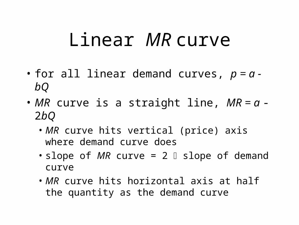
• for all linear demand curves, p = a - bQ
• MR curve is a straight line, MR = a - 2bQ• MR curve hits vertical (price) axis where
demand curve does• slope of MR curve = 2 slope of demand curve• MR curve hits horizontal axis at half the
quantity as the demand curve

In our example
• p = 24 – Q• so a = 24 and b = 1 p /Q = -1
• hence MR = p + (p/Q) Q
= (24 – Q) + (-1) Q
= 24 – 2Q

Using calculus
R(Q) = p(Q)Q
if linear:
R(Q) = [a - bQ]Q = aQ - bQ2
MR = dR/dQ = a - 2bQ

MR and elasticity of demand
• MR at any given quantity depends on• demand curve's height (price)• demand curve's shape (elasticity)
• thus, it depends on its elasticity

Derive MR/elasticity formula
• demand elasticity:
= (Q/Q)/(p/p) = (Q/p)(p/Q)
• MR = p + (p/Q) Q
= p + (p/Q)(Q/p)p1
1p

MR and price
• MR
• MR closer to p the more elastic is demand• where demand curve hits price axis (Q = 0),
demand curve is perfectly elastic MR = p• MR = 0 where demand elasticity is = -1• MR < 0 where demand is inelastic: 0 > -1
11p

Table 11.1 Quantity, Price, Marginal Revenue, and Elasticity for the Linear Inverse Demand Curve p=24-Q

Figure 11.2 Elasticity of Demand and Total, Average, and Marginal Revenue
p, $ per unit
Demand ( p = 24 – Q)
Perfectly elastic
Perfectlyinelastic
Elastic, < –1
Inelastic, –1 < < 0
= –1
p = –1
Q = 1Q = 1
MR = –2
Q, Units per day
24
12
0 12 24MR = 24 – 2Q

Choosing price or quantity
• monopoly can set p or Q to maximize its profit, • monopoly is constrained by market demand curve
• it cannot set both Q and p (cannot pick a point above demand curve)
• if monopoly sets p, demand curve determines Q
• if monopoly sets Q, demand curve determines p
• because monopoly wants to maximize , it chooses same profit-maximizing solution whether it sets p or Q

Profit maximization
all firms, including monopolies, use a two-step analysis
1. firm determines output, Q*, at which it makes highest , where
• MR = MC• in elastic portion of demand curve
2. firm decides whether to produce Q* or shut down: p AVC

Figure 11.3 Maximizing Profit
12
18
24
8
6
108
144
60
60 12 24
R, , $
0 126 24
AC
AVCe
Demand
= 60
MC
MR
Q, Units per day
Revenue, R
Profit,
Q, Units per day
p, $ per unit
(a) Monopolized Market
(b) Profit, Revenue

SR cost in our example
• C(Q) = Q2 + 12
• MC = dC(Q)/dQ = 2Q
• AVC = VC/Q = Q2/Q = Q
• AC = C/Q = (Q2 + 12)/Q = Q + 12/Q

Profit is maximized where
• MR = 24 – 2Q = 2Q = MC
Q = 6
• inverse demand: p = 24 – Q = 24 – 6 = 18
• AVC = Q = 6 < p = 18 so produce > 0 because AC = Q + 12/Q = 8 < p = 18

Market power
ability of a firm to charge a price above marginal cost profitably

No check on bank market power
banks exercise substantial market power on the rate for bounced checks
• although you had no idea that a check wouldn't clear, bank charges you an average of $4.75 to $7.50 (up to $10)
• large banks charge more than small ones• bad check writer also pays an average of
$15 to $19.50 (up to $30)

Bank costs
• bank's handling fees for bad checks = $1.32• most checks eventually clear (check writer
merely miscalculated balances)• even including losses from fraud, total MC
= $2.70 (Center for the Study of Responsive Law)
• thus, banks are exercising substantial market power: price > MC

Market power and shape of demand curve
• market power depends on shape of demand curve (elasticity)
• at profit-maximizing quantity:
11MR p MC
1
1 1/
p
MC
Lerner index (price markup)
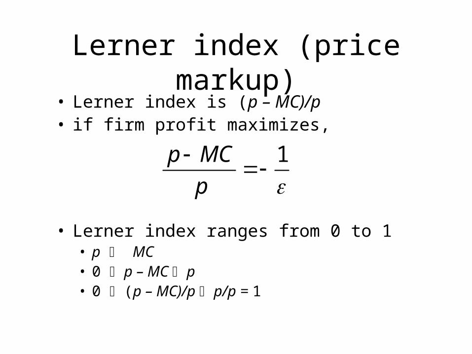
1p MC
p
• Lerner index is (p – MC)/p• if firm profit maximizes,
• Lerner index ranges from 0 to 1• p MC• 0 p – MC p• 0 (p – MC)/p p/p = 1


Causes of market power
monopoly's demand curve is relatively inelastic if
• consumers are willing to pay "virtually anything" for it
• no close substitutes for firm's product exist• other firms can't enter market• other similar firms are located far away• other firms’ products very different

Welfare effects of monopoly
• welfare = consumer surplus + producer surplus
• W = CS + PS
• welfare is < under monopoly than under competition
• monopoly sets p > MC, causing deadweight loss (DWL)

= 18
Figure 11.5 Deadweight Loss of Monopoly
p, $ per unit
Demand
Q , Units per day
MR
MC
pc = 16B = $12
D =$60
C =$2
E = $4MR = MC = 12
A = $18pm
24
Q m = 6 Q c = 8 24120
em
ec

Solved problem
• in our linear example,
• how does subjecting a monopoly to a specific tax of = $8 per unit affect• monopoly optimum • welfare of consumers, the monopoly, and
society?
• what is tax incidence on consumers?

Solved Problem 11.1
p, $ per unit
Demand
Q, Units per day
MR
MC1 (before tax)
MC2 (after tax)
p1 = 18
D E
C
F
G
B
A = $8
0
8
p2 = 20
24
Q2 = 4 Q1= 6 2412
e1
e2

Competitive vs. monopoly sugar tax incidence
• incidence of a tax on consumers may be less for a monopolized than a competitive market
• in 1996, Florida voted on (and rejected) a one-cents-per-pound excise tax on refined cane sugar in the Florida Everglades Agricultural Area
• given linear supply (or marginal cost) and demand curves the tax incidence on consumers from this tax is• 70% if the market is competitive• 41% if monopolistic
• thus, a competitive Florida sugar industry passes on substantially more of the tax to demanders than it would if the industry were monopolized

Welfare effects of taxes
• governments use ad valorem taxes (p per unit) more often than specific taxes ( per unit) – why?
• suppose both taxes cut output by the same amount
• which one raises the most government tax revenue?

Figure 11.6 Ad Valorem Versus Specific Tax
p, $ per unit
A
B
Before-taxdemand, D
Q, Units per year
MR
MC
e1
e2
p2
p1
pa = (1 – )p2
ps = p2 –
Q2 Q1 MRa
Da
MRs
Ds

Why monopolies?
• firm has cost advantage over others firms
• government created monopoly
• merger of several firms into a single firm
• firms act collectively: cartel
• strategies - such as threats of violence - that discourage other firms from entering market

Sources of cost advantages
• firm controls a key input:
• essential facility: scarce resource that rival needs to use to survive• firm knows of superior technology, or • has better way of organizing production

Natural monopoly
• market has a natural monopoly if one firm can produce total market output at lower cost than could several firms
• if cost for Firm i to produces qi is C(qi), condition for a natural monopoly is
C(Q) < C(q1) + C(q2) + ... + C(qn),• where Q = q1 + q2 + .. + qn is sum of output
of any n > 2 firms

Sufficient condition
natural monopoly if
• AC curve falls at any observed quantity for all firms
• economies of scale

Electricity example
• F = $60 (build plant & connect houses)
• MC = m = $10 (constant)
• AC = m + F/Q = 10 + 60/Q, declines as output rises

Costs of producing Q = 12
# of firms output AC = 10+60/Q C
1 12 $15 $180
2 6 $20 $240
having only one firm produce avoids a
second fixed cost (MC doesn’t vary with
number of firms)

Figure 11.7 Natural Monopoly
15
20
40
10
60 12 15
AC = 10 + 60/Q
MC = 10
Q, Units per day
AC, MC,$ per unit

Public utilities
apparently believing they’re natural monopolies, governments grant monopoly rights for essential good or service “public utilities”
• water• gas• electric power• mail delivery
Electric power utilities
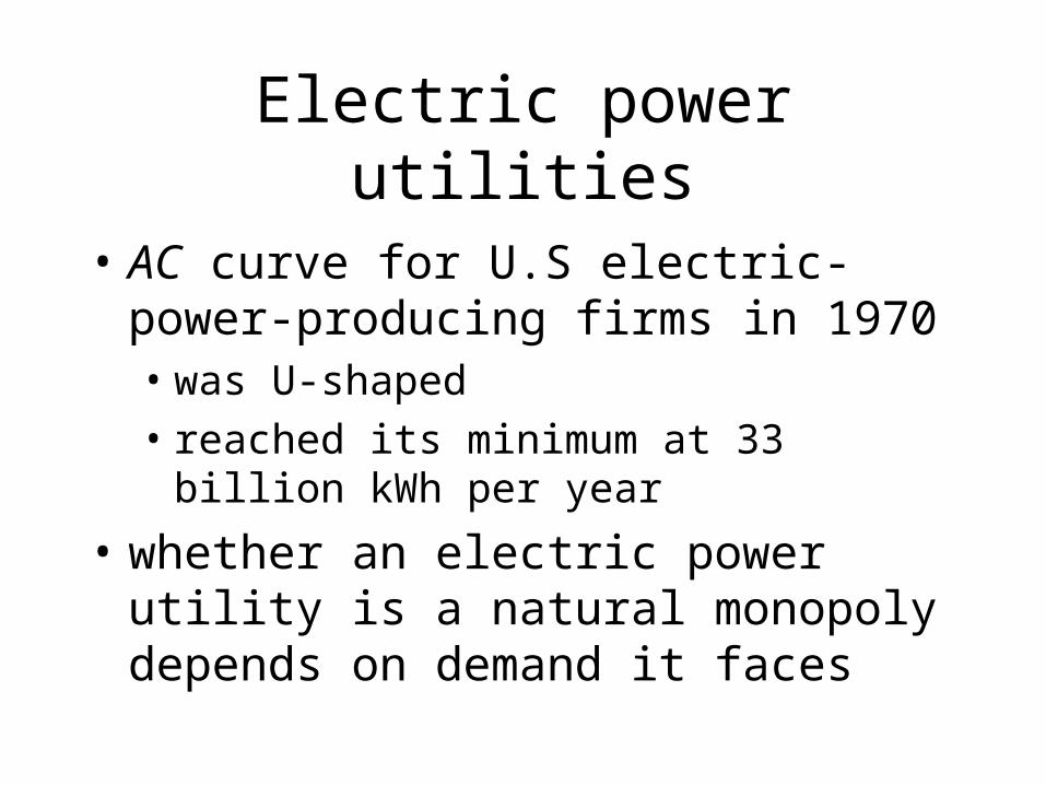
• AC curve for U.S electric-power-producing firms in 1970 • was U-shaped • reached its minimum at 33 billion kWh per year
• whether an electric power utility is a natural monopoly depends on demand it faces

Economies of scale
• natural monopolies: most electric companies operated in regions of substantial economies of scale• Newport Electric produced 0.5 billion kWh/year• Iowa Southern Utilities: 1.3 billion kWh/year
• not natural monopolies: a few operated in upward-sloping section of AC curve• Southern produced 54 kWh/year• 2 firms could produce that quantity at 3¢ less per
thousand kWh than could a single firm

Application Electric Power Utilities
4.85
5.10
4.79
Cost, $ perthousand kWh
0 33 66Q , Billion kWh per year
AC
D

Government created monopolies
• barriers to entry (e.g, patents)• own and manage many monopolies
• postal services• garbage collection• utilities
• electricity• water• gas• phone services

Barriers to entry
governments prevent other firms from entering a market in 3 ways
• by making it difficult for new firms to obtain a license to operate
• by granting a firm rights to be a monopoly
• by auctioning rights to be a monopoly

Patents
• grants an inventor right to be monopoly provider of good for a number of years
• stimulates research

Iceland’s government creates genetic monopoly
• starting in 874, Viking crews from western Norway grabbed young Celtic women from Ireland and took them to Iceland
• 11 centuries later, the descendents of these 10,000 to 15,000 pirates and their about five-times-as-many slave wives form an unusually isolated population with a relatively homogeneous gene pool
• Iceland has tissue samples dating back to the 1940s and meticulous records on every citizen since 1915
• careful genealogic records have been kept that allows researchers to trace disease genes back more than 10 generations

deCODE Genetics • Dr. Kari Stefansson believed that the unique genetic dataset
of the 286,000 current Icelanders (and their forbearers) would help pinpoint genetics of some serious common diseases
• he formed a firm, deCODE Genetics• in 1998, deCODE acquired 12 years of monopoly rights to
the genetic, medical, and genealogical records of Iceland for about $200 million
• the firm agreed to provide Icelanders for free with drugs and diagnostic tools stemming from their research
• the firm has collected voluntary blood samples from tens of thousands of people to augment their databases
• by 2002, deCODE announced findings for a number of diseases and had revenues of $13.4 million

Drug patent: Botox
• Dr. Alan Scott turned a deadly poison, botulinum toxin, into a miracle drug to treat• strabismus, or cross-eyes, which affects about
4% of children• blepharospasm, an uncontrollable closure of the
eyes, which left about 25,000 Americans functionally blind before his discovery
• his patented drug, Botox, is sold by Allergan Inc.

Other uses
• Dr. Scott has been amused to see several of the unintended beneficiaries of his research at the Academy Awards
• even before it was explicitly approved for cosmetic use, many doctors were injecting Boxtox into the facial muscles of actors, models, and other people to smooth out their wrinkles
• ideally for Allergan, the treatment is only temporary, lasting up to 120 days, so repeated injections are necessary

Profits
• Allergan had expected to sell $400 million worth of Botox in 2002
• however, in April 2002, the FDA approved Botox for cosmetic purposes—allows Allegran to advertise the drug widely
• The firm expects Botox to eventually earn a $1 billion a year (becoming another Viagra)

Compare
• Mattel sold $1.4 billion worth of Barbie dolls over 37 years

Justification
• patent monopoly profits spur new research
• people benefit greatly from many inventions (new drugs)

Botox profit maximization
• Dr. Scott can produce a vial of Botox in his lab for about $25
• Allergan sells a vtal to doctors for about $400• assuming that the firm is setting its price to maximize its
short-run profit, the elasticity of demand for Botox is determined by:
• thus, demand it faces is only slightly elastic
4001.067.
400 25
p
p MC

Linear demand
• if the demand curve is linear and elasticity of demand is ‑1.067 at 2002 monopoly optimum (1 million vials sold at $400 each), Allergan’s inverse demand function is
p = 775 – 375Q.• demand curve:
• slope is -375• hits price axis at $775• hits quantity axis at 2.07 million vials per year
• corresponding marginal revenue curve isMR = 775 – 750Q,
• strikes the price axis at $775• has twice the slope, -750, as the demand curve

Monopoly optimum
• intersection of the marginal revenue and marginal cost curves,
MR = 775 – 750Q = 25 = MC,
• determines the monopoly equilibrium at the profit-maximizing quantity of 1 million vials per year and a price of $400 per vial

25
400
p , $ per vial
Q , Millions vials of Botox per year1
A = $187.5 million
MC = AVC
Demand
MR2
775
2.07
e c
e m
B = $375 million C = $187.5 million

Botox Benefits
• SR relief from eye problems and wrinkles (CS at monopoly price):
A = $187.5 million per year• LR CS after patent expired (buy at MC):
A + B + C = $750 million per year• Patent monopoly profit (ignoring fixed costs):
B = $375 million per year

Auctions
• Oakland cable TV• SF auctioned monopoly rights to store cars towed
for illegal parking• monopoly, City Tow, collects $40 per car, of which
$15.03 goes to the city
• losing company's bid promised the city only $7.50
• ASUC tried to create a bookstore monopoly without holding an auction

Government actions that reduce market power
• antitrust laws prohibit monopolization, price fixing, and so forth
• regulations prevent monopolies from exercising all of their market power

Optimal price regulation
• price regulation may eliminate DWL
• regulation is optimal if it leads to "competitive" outcome

Figure 11.8 Optimal Price Regulation
p , $ per unit
Regulated demand
Market demand
Q , Units per day2412860
MRMR r
MC
18
24
16
DE
CB
A em
eo

Nonoptimal price regulation
• welfare is reduced if government does not set price optimally
• if regulated p is < minimum of monopoly's AVC, monopoly shuts down
• if regulated price is between shut-down point and monopoly price but not equal to competitive price• too little is produced
• welfare is below competitive level

Figure 11.9 Regulating an Electric Utility
p, Yen (¥) perhundred KWH
31230 34 54
A
B
Demand
Q, Billion kWh per year
30.3
26.9
22.321.919.5
MR
ACMC
53
e1
e2
e3

Solved problem 11.3
What's the effect of a price regulation on a monopoly that is below the competitive price?

Solved Problem 11.3
p, $ per unit
Regulated demand
Market demand
Q, Units per day
MRMR
MC
p1 D
E
C
BA
p2
Q 2 Q1 Qd
e1
e2
Excess demand
r

Creation and destruction of an aluminum monopoly
• cost advantages and government actions gave Aluminum Company of America (Alcoa) a U.S. monopoly in aluminum
• monopoly lasted for decades

Alcoa becomes a monopoly
• Alfred Hall invented and patented a new process in 1893
• allowed his firm, Pittsburgh Reduction (which became Alcoa) to produce aluminum at much lower cost than competitors
• this firm controlled most domestic and many international sources of bauxite ore
Alcoa was only American producer of aluminum
WWI to WWII
• Alcoa faced some competition from foreign producers, but U.S. established high tariffs on aluminum imports
• during WWI, when foreign competitors were unable to effectively produce and sell in other countries, Alcoa became an exporter
• Alcoa continued to export after war• between WWI and WWII, Alcoa remained only
aluminum smelter (producer) in U.S. due to its technological advantages and economies of scale

WWII
• demand for aluminum increased substantially with start of WWII
• aluminum was used to produce planes and other manufactured products for the war effort.
• during WWII, government financed new plants that were built and run by Alcoa and encouraged development of other aluminum producers

Break up
• at end of WWII in 1945, U.S. Supreme Court ruled Alcoa monopoly should be broken up
• government-financed Alcoa plants sold at low prices to Reynolds Metals Company & Permanente Metals Corporation (owned by Henry Kaiser) creating oligopoly by 1950• Alcoa: 50.9% of all sales• Reynolds: 30.9%• Kaiser Aluminum & Chemical Corporation (renamed
Permanente Metals): 18.2%

Textbook prices
• textbook authors tell students that they urge the publisher to charge lower prices
• are they telling the truth?

Sharing textbook revenues
• college-textbook publishers usually pay authors a royalty: fraction of wholesale revenues
• why pay a percentage of revenues rather than• lump-sum payment• percentage of profit?
Explanations
• neither authors nor publishers can accurately forecast sales, hence agreeing on a lump-sum payment is difficult
• authors don't want a percentage of profit because they don't trust publishers to accurately report profit

Maximizing joint profit
Which royalty method(s) maximizes joint profit: sum of publisher’s and author’s profit?
Author’s royalty is a
A. fraction of revenue
B. fraction of economic profit
C. lump-sum payment

Problem with revenue sharing
• leads to inefficiency: too few books are sold
• no inefficiency with • lump-sum fee • percentage of profit

Lump-sum fee
• if publisher paid author fixed fee, L, publisher would get residual profit
• hence publisher has an incentive to maximize joint profit,
• number of books that maximizes joint profit, Q*, maximizes residual profit, - L
• to sell Q*, publisher must set optimal price p*

Profit, $
0
, Joint profit
Books per year
– L,
Publisher’s profit
’
E *
E
Q*

Percentage of joint profit
• if used, publisher would set price to maximize joint profit, , which maximizes both parties’ shares
• however, authors do not trust publishers to truthfully report economic profit• even without falsifying its accounts, publisher can
report very low profit• because many costs of publishing are shared across
textbooks (joint product)
• authors put more trust in reported revenue

Model
• demand for textbook is downward sloping• so there is some market power• rival texts limit the market power
• constant marginal cost


Dominant firm/competitive fringe
• dominant firm (DF): a price-setting firm that competes with price-taking firms (competitive fringe)
• DF maximizes its profit given • its cost curves and • demand curve it faces• (before fringe enters, DF faces market demand)

Residual demand curve
after entry, DF faces residual demand curve: the market demand that is not met by other firms (competitive fringe) at any given price:
Dr(p) = D(p) – Sf(p)
where Sf is fringe’s supply curve

Figure 11.10 Dominant Firm-Competitive Fringe Equilibrium
p, $ per unit
Q, Units of output per year
MCd
Dr
Sf
MRr
ef d
D
Q*dq*
dQ*f
p1
p*
p2

1. Monopoly profit maximization
• chooses p or Q
• maximizes profit where MR = MC
• operates if p AVC

2. Market power
• ability of a firm to charge a price above MC and earn a positive profit
• more elastic is demand at Q where monopoly maximizes its profit• closer is its p to its MC• closer is Lerner Index, (p - MC)/p, to zero
(competitive level)
3. Welfare effects of monopoly
• because a monopoly's p > MC
• too little output is produced
• society suffers a DWL
• consumers are worse off
• monopoly's profit > competitive level

4. Cost advantages that create monopolies
firm may become a monopoly if it
• controls a key input
• has superior knowledge about producing or distributing a good
• has substantial economies of scale
• in markets with substantial economies of scale, single seller is a natural monopoly
5. Government actions that create monopolies
• governments may establish
• government-owned and operated monopolies
• private monopolies by
• establishing barriers to entry
• patents

6. Government actions that reduce market power
• government can eliminate welfare harm of a monopoly by forcing firm to set its price at competitive level
• government can eliminate or reduce harms of monopoly by allowing or facilitating entry