chapter 11: variable stars, light curves & periodicity variable star astronomy – chapter 11...

Chapter 11: Variable Stars, Light Curves & Periodicity

Introduction

Variable stars are, quite simply, stars that change brightness. More than 30,000 are known and catalogued, and many thousands more are suspected variables. Their light variations are a vital clue to their nature, but professional astronomers do not have the time or the telescopes to monitor the brightness of thousands of variables night after night; their efforts are directed toward understanding specific aspects of the stars using such sophisticated instruments as spectrographs, photometers, radio telescopes, and satellites. Such instruments enable us to probe many different regions of the spectrum, such as X-rays, ultraviolet, infrared, and radio wavelengths. Yet it is crucial to measure the stars in ordinary visual light (the optical region of the spectrum) as well. The data obtained with special instruments and in shorter or longer wavelengths of light are compared with optical measurements , which serve as a

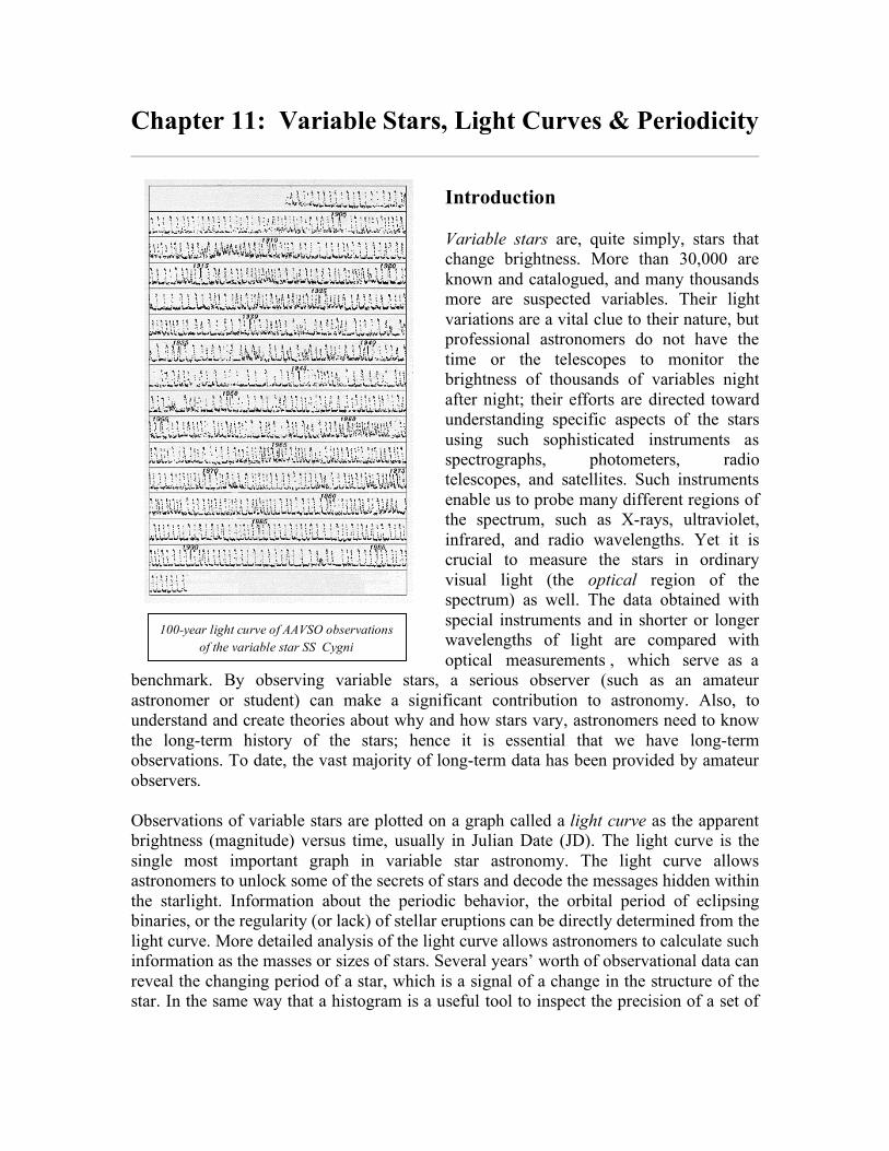
benchmark. By observing variable stars, a serious observer (such as an amateur astronomer or student) can make a significant contribution to astronomy. Also, to understand and create theories about why and how stars vary, astronomers need to know the long-term history of the stars; hence it is essential that we have long-term observations. To date, the vast majority of long-term data has been provided by amateur observers. Observations of variable stars are plotted on a graph called a light curve as the apparent brightness (magnitude) versus time, usually in Julian Date (JD). The light curve is the single most important graph in variable star astronomy. The light curve allows astronomers to unlock some of the secrets of stars and decode the messages hidden within the starlight. Information about the periodic behavior, the orbital period of eclipsing binaries, or the regularity (or lack) of stellar eruptions can be directly determined from the light curve. More detailed analysis of the light curve allows astronomers to calculate such information as the masses or sizes of stars. Several years’ worth of observational data can reveal the changing period of a star, which is a signal of a change in the structure of the star. In the same way that a histogram is a useful tool to inspect the precision of a set of

100-year light curve of AAVSO observations of the variable star SS Cygni

AAVSO Variable Star Astronomy – Chapter 11

measurements, we can visualize the nature of a star’s variation more easily by plotting a light curve of apparent magnitude versus time.

Light curves show that many variable stars are periodic. Periodic phenomena repeat in a regular way that is predictable. However, the line between periodic phenomena and non-periodic phenomena is not always a sharp one. Sometimes a process may seem to be periodic from a large-scale perspective, while investigation on a fine scale reveals non- periodic variations. Consider the change in apparent altitude of the Sun. If you measure the highest apparent altitude of the Sun each day for a week, you will not notice much change. The Sun seems to reach the same maximum altitude each day. Over a period of a month, however, changes will become obvious. But if we take measurements each day from December 31st until the summer solstice around June 21st, the apparent daily altitude of the Sun gets higher and higher. This is still non-periodic behavior. If we take our measurements for an entire year, from December 31st to December 31st, we will see a definite pattern. When we examine the change in the apparent altitude of the Sun over several years, we see that in addition to monthly variations, it follows a regular pattern with a period of one year.

Many variable stars do exhibit simple periodic behavior. Some semiregular variables have time intervals of periodic behavior in between non-periodic intervals. Some have two separate periodic cycles superimposed over each other, affecting the overall result. The only way to determine the periodicity is by plotting and analyzing light curves. The emerging patterns will then tell their story.

There are four main classes of variable stars: pulsating and eruptive variables whose variability is intrinsic—due to physical changes in the star or stellar system; and eclipsing binary and rotating stars whose variability is extrinsic—due to an eclipse of one star by another or the effect of stellar rotation. Below is a brief description of several different types of variable stars with their corresponding light curves. There is also more detailed information about some of the variables mentioned below throughout the Hands-On Astrophysics manual. A general discussion of variables is the focus of the Space Talk in Chapter 5 (pp. 87–88); the Space Talk in Chapter 7 (pp. 118–121) is about Cepheids and the distance scale; the Space Talk in Chapter 12 (pp. 225–228) is about omicron Ceti (Mira); Poster Page 12.1 in Chapter 12 features SS Cygni; and Poster Page 13.1 in Chapter 13 is about beta Persei (Algol). In addition, a summary of the different types of variable stars is included in the Appendix, and a discussion of variable stars is presented in the accompanying HOA video entitled Variable Stars.


I. Intrinsic Variable Stars A. Pulsating Variable Stars Pulsating variables change brightness because they change their size and/or shape; the whole star is actually “vibrating.” Most of them simply expand and contract repeatedly, swelling and shrinking in a continuing cycle of size changes; this is known as the fundamental mode of pulsation. Others change not only their size, but the internal arrangement of material within the star as well. Still others change shape, alternately flattening and elongating, or showing even more complex shape changes. And to make things yet more complicated, some stars vibrate in more than one way (more than one mode) at the same time. Like most vibrating systems, pulsating variables repeat their changes; they tend to be periodic. (See the Space Talk in Chapter 12, pp. 225–228.)

One important class of pulsating variables is the Cepheid variables. These large yellow stars pulsate with periods from 1 to 70 days, with an amplitude of light variation up to 2 magnitudes. They are intrinsically very bright (high luminosity). The greater the absolute magnitude (luminosity) of a Cepheid, the longer its period. In fact, there is a strict relationship between a Cepheid’s period and its luminosity, called the period-luminosity relationship. We can determine the period of a Cepheid from its light curve; then, using the period of the Cepheid, we can apply the period-luminosity relationship to compute the Cepheid’s luminosity. Knowing its magnitude (how bright it appears to observers on Earth) and its luminosity (how bright it actually is) allows us to compute its distance from us, thereby enabling us to use Cepheid variables as distance markers. For example, just as astronomers in the first half of this century used Cepheid variables within the Milky Way itself to measure distances within our own galaxy, we can measure the distance to any given galaxy by computing the distance to its Cepheid variables. (See also the discussion in the Space Talk in Chapter 7, pp. 118–121.)

The light curve for the Cepheid variable X Cygni is shown below; each dot represents one observation. (All observations of X Cyg, and all subsequent light curves come from the AAVSO International Database, unless otherwise noted.) One of the largest groups of pulsating variables is the long-period variables, or LPVs. They are further divided into two major subclasses, the Mira-type and the semiregular variables. The visual light curves of Mira-type variables show well-defined periods ranging from 80 to nearly 1000 days, with amplitudes of 2.5 magnitudes or more. Mira- type variables are red giant stars, often of enormous size. Many of them are slowly


ejecting a steady stream of matter into the surrounding space; this mass loss can have very dramatic consequences for their future evolution. This class of variable is named after the star Mira (also known as omicron Ceti), the first such star discovered (see the Space Talk in Chapter 12, pp. 225–228); its light curve is shown below.

Yet another group of pulsating stars is the semiregular variables. These giants and supergiants show appreciable periodicity accompanied by intervals of irregular light variation. The periods range from 30 to 1000 days, with light amplitudes of not more than one to two magnitudes. An example is Z Ursae Majoris. RV Tauri stars are also variables that pulsate. These yellow supergiants have a characteristic light variation with alternating deep and shallow minima. Their periods, defined as the interval between two deep minima, range from 30 to 150 days. The light amplitude may vary as much as four magnitudes. Many of these variables show long- term cyclic variations in brightness from hundreds to thousands of days. An example of an RV Tauri variable star light curve is that of R Scuti.


B. Eruptive (Cataclysmic) Variable Stars Another major category of variables is the eruptive variables. These are not one-star systems, but two stars orbiting very close to each other, one of them a normal Sun-like or giant star, the other a white dwarf star. White dwarf stars are very compressed: they may pack the mass of our entire Sun into a size no bigger than the Earth. Some of the outermost material from the larger star is pulled away by the white dwarf’s gravity, but this material does not fall directly onto the white dwarf. Instead, it builds up in a disk called an accretion disk, which orbits the white dwarf. The combination of normal or giant star, white dwarf, and accretion disk can lead to some very spectacular celestial fireworks. That is why, instead of varying smoothly like most pulsating variables, eruptive variables exhibit outbursts of activity, usually brightening by a large amount. The changes in their light curves are usually very unpredictable, and tend to be sudden and dramatic; that is why these stars are also called “cataclysmic variables.” Novae explosions (eruptions) occur in close binary systems consisting of a white dwarf orbiting a larger and cooler star. A layer of hydrogen-rich material is slowly accreted from the cooler star onto the compact white dwarf. The accreted material provides the fuel for the nova explosion—a thermonuclear fusion reaction similar to the detonation of a hydrogen bomb. The system increases in brightness by 7 to 16 magnitudes in a matter of one to several hundred days. After the eruption, the light slowly fades back to its original brightness over several years or decades, as shown in the light curve of V1500 Cygni at right. Systems which have undergone two or more nova-like eruptions during their recorded history are referred to as recurrent novae. Such recurrent eruptions have a slightly smaller amplitude than that which is observed in novae. An example of a recurrent nova is RS Ophiuchi.


Yet another class of cataclysmic variable stars is called dwarf novae. These are close binary systems made up of a Sun-like star, a white dwarf, and an accretion disk surrounding the white dwarf. As matter accumulates in the accretion disk, the disk becomes unstable. Eventually, matter from the unstable disk will fall onto the white dwarf, leading to an outburst. There are three sub-classes of dwarf novae.

Dwarf novae of the U Geminorum sub-class (also called SS Cygni sub-class) are also in close binary systems, with orbital periods on the order of a few hours. After intervals of well-defined quiescence at minimum magnitude, they brighten suddenly within 1–2 days. Depending on the star, the eruptions occur at intervals of 30 to 500 days. The light amplitude of the outbursts ranges from two to six magnitudes with a duration of 5 to 20 days. An example is SS Cygni. Z Camelopardalis stars, the second dwarf novae sub-class, are physically similar to U Geminorum stars. Their eruptions occur at intervals of 10 to 30 days or more; however, the quiescent level of Z Camelopardalis stars is not well-defined. In addition, the cyclic variations are interrupted by intervals of constant brightness called standstills (also called stillstands). The standstills last the equivalent of several cycles (sometimes years), with the star “stuck” at a brightness approximately a third of the way from maximum to minimum. In general, at the end of a standstill, the star continues to fade to its quiescent level, as in the light curve of the prototype star Z Camelopardalis, below. SU Ursae Majoris stars, the third dwarf novae sub-class, are also physically similar to U Geminorum stars. They have short orbital periods of less than two hours. In addition, they have two distinct kinds of outbursts: one is short, with a duration of one to several days, faint and more frequent; the other (superoutburst) is long, with a duration of 10 to 20 days, bright and less frequent. During superoutbursts, small-amplitude, periodic


modulations (superhumps) appear with periods two to three percent longer than the orbital period of the system. The light curve of SU Ursae Majoris appears below; can you find the superoutburst? Another group of eruptive variables is the symbiotic stars, which display semiperiodic nova-like outbursts of up to four magnitudes. These are close binary systems with one component a red giant and the other a hot blue star. They are embedded in nebulosity, a region of gas and dust. An example is Z Andromedae. R Coronae Borealis variables are high-luminosity stars (supergiants) which go into “outburst” not by brightening, but by fading! They spend most of their time at maximum magnitude, and at irregular intervals fade by one to nine magnitudes, slowly recovering to their maximum magnitude after a few months or years. The drop in brightness is believed to be caused by the formation of soot in the star’s atmosphere, which is abnormally rich in carbon. When the carbon veil is blown away, the star returns to maximum magnitude. The light curve (one-day means) of R Coronae Borealis is shown below.


Perhaps the most spectacular of all variables is the supernova. A supernova is the violent end of a massive star during which the star quite literally explodes, blasting most of its material out into space in seconds. As a result, it can brighten by 20 magnitudes or more; a large supernova may briefly outshine the entire rest of the galaxy. The tremendous explosion will leave behind a fragment of very dense material at its center. This may take the form of a neutron star, whose material is compressed to the density of an atomic nucleus. Or it may be so compressed that it forms a black hole, a region where the gravity is so strong that nothing, not even light, can escape.

The light curve of the spectacular Supernova 1987A, which appeared in 1987 in the Large Magellanic Cloud (a dwarf galaxy near our own Milky Way), is shown above. The material blown off in a supernova explosion is rich in complex elements such as carbon, nitrogen, oxygen, and iron. Eons later, this material can condense as part of a newly-forming star system. The enrichment of our galaxy by supernova explosions has provided the necessary complex elements to form Earth-like planets, and even life. It is no exaggeration to say that we are stardust: many atoms in our bodies, including carbon, calcium, iron, and magnesium, were synthesized within the core of a star, and probably ejected by a supernova explosion.

A supernova happens, on average, about every 300 years in a galaxy. The last supernova in our own galaxy was in the year 1054, over 900 years ago. Are we overdue? Stars vary when they are in the stages of birth, old age, or death, all of which are periods of extreme instability in the life of a star. Many pulsating variables, for example, are near the end of their lives, and running out of their main fuel, hydrogen. Thermonuclear fusion does not simply turn on at birth and quietly turn off when the hydrogen is exhausted: fuels other than hydrogen can be burned, causing a wide variety of nuclear reactions and changes to the star’s structure. The changes in the fuel economy of a star can upset the delicate balance between gravity and radiation pressure which has kept the star stable for most of its lifetime. Through the variations in their brightness, these stars “talk” to us—they try to tell us their story. Thus by studying variable stars, astronomers try to put together the puzzle of how stars evolve and die.


II. Extrinsic Variable Stars A. Eclipsing Binaries Eclipsing binaries are binary star systems whose members eclipse each other, blocking one another’s light, thereby causing the system to look fainter to observers on Earth. The light curve of an eclipsing binary depends on the sizes and brightnesses of the stars, their separation from each other, and the geometry of our view from Earth. For example, the first star may be larger, and totally eclipse the second, while the second only partially eclipses the first. The time between primary eclipses is the orbital period of the binary system. Detailed analysis of the light curve shape yields much information about the size, mass, and shape of the stars, and the shape of their orbits. Beta Persei (Algol), whose folded light curve is shown below, is an eclipsing binary that can be seen with the unaided eye. (Folded light curves, or phase diagrams, have two or more cycles superimposed on each other. They will be examined in greater detail in Chapter 12.) B. Rotating Variables Rotating variables are rapidly rotating stars, often in binary systems, that undergo small-amplitude changes in light which may be due to dark or bright spots on the star’s surface, similar to sunspots on our own Sun.


Investigation 11.1: Recognizing Periodic Curves

A periodic curve is one which repeats identically within a fixed time interval. Study the following curves and determine which ones seem to exhibit periodic behavior. Determine the maxima, the minima, and the periods. From the description of the types of variable stars included with this investigation, what type(s) of variable star(s) do you think each light curve represents?


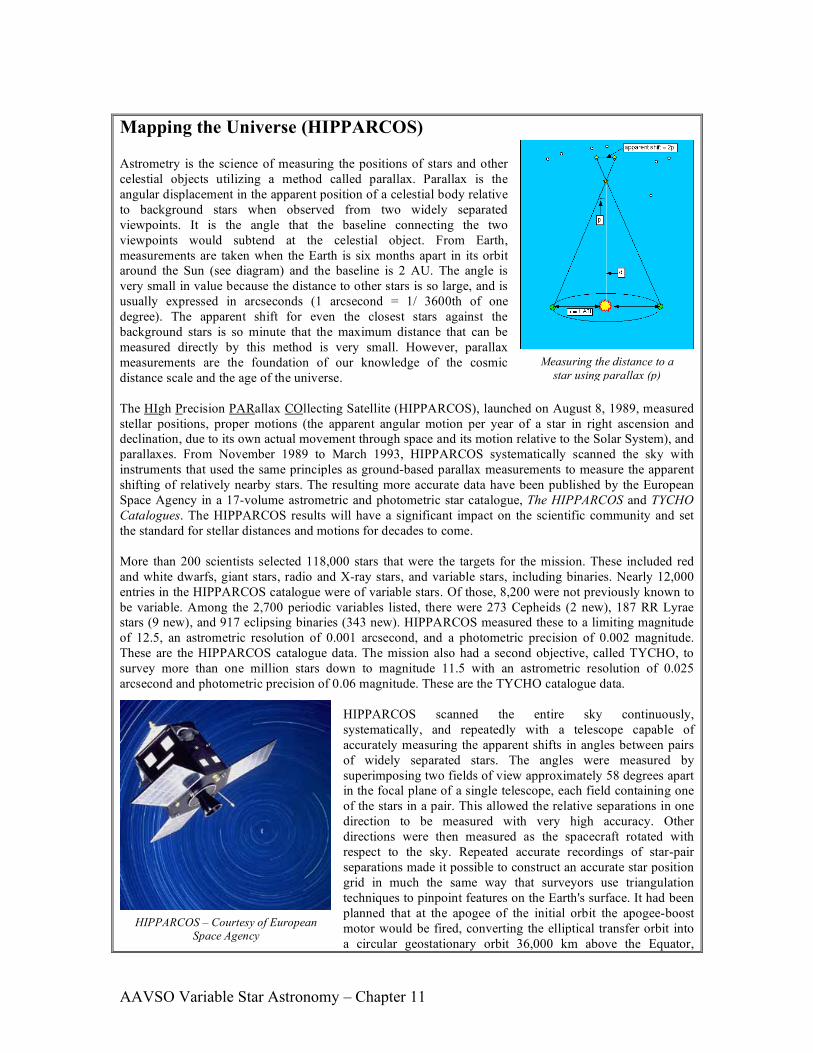
Mapping the Universe (HIPPARCOS) Astrometry is the science of measuring the positions of stars and other celestial objects utilizing a method called parallax. Parallax is the angular displacement in the apparent position of a celestial body relative to background stars when observed from two widely separated viewpoints. It is the angle that the baseline connecting the two viewpoints would subtend at the celestial object. From Earth, measurements are taken when the Earth is six months apart in its orbit around the Sun (see diagram) and the baseline is 2 AU. The angle is very small in value because the distance to other stars is so large, and is usually expressed in arcseconds (1 arcsecond = 1/ 3600th of one degree). The apparent shift for even the closest stars against the background stars is so minute that the maximum distance that can be measured directly by this method is very small. However, parallax measurements are the foundation of our knowledge of the cosmic distance scale and the age of the universe. The HIgh Precision PARallax COllecting Satellite (HIPPARCOS), launched on August 8, 1989, measured stellar positions, proper motions (the apparent angular motion per year of a star in right ascension and declination, due to its own actual movement through space and its motion relative to the Solar System), and parallaxes. From November 1989 to March 1993, HIPPARCOS systematically scanned the sky with instruments that used the same principles as ground-based parallax measurements to measure the apparent shifting of relatively nearby stars. The resulting more accurate data have been published by the European Space Agency in a 17-volume astrometric and photometric star catalogue, The HIPPARCOS and TYCHO Catalogues. The HIPPARCOS results will have a significant impact on the scientific community and set the standard for stellar distances and motions for decades to come. More than 200 scientists selected 118,000 stars that were the targets for the mission. These included red and white dwarfs, giant stars, radio and X-ray stars, and variable stars, including binaries. Nearly 12,000 entries in the HIPPARCOS catalogue were of variable stars. Of those, 8,200 were not previously known to be variable. Among the 2,700 periodic variables listed, there were 273 Cepheids (2 new), 187 RR Lyrae stars (9 new), and 917 eclipsing binaries (343 new). HIPPARCOS measured these to a limiting magnitude of 12.5, an astrometric resolution of 0.001 arcsecond, and a photometric precision of 0.002 magnitude. These are the HIPPARCOS catalogue data. The mission also had a second objective, called TYCHO, to survey more than one million stars down to magnitude 11.5 with an astrometric resolution of 0.025 arcsecond and photometric precision of 0.06 magnitude. These are the TYCHO catalogue data.

HIPPARCOS scanned the entire sky continuously, systematically, and repeatedly with a telescope capable of accurately measuring the apparent shifts in angles between pairs of widely separated stars. The angles were measured by superimposing two fields of view approximately 58 degrees apart in the focal plane of a single telescope, each field containing one of the stars in a pair. This allowed the relative separations in one direction to be measured with very high accuracy. Other directions were then measured as the spacecraft rotated with respect to the sky. Repeated accurate recordings of star-pair separations made it possible to construct an accurate star position grid in much the same way that surveyors use triangulation techniques to pinpoint features on the Earth's surface. It had been planned that at the apogee of the initial orbit the apogee-boost motor would be fired, converting the elliptical transfer orbit into a circular geostationary orbit 36,000 km above the Equator,

Measuring the distance to a star using parallax (p)

HIPPARCOS – Courtesy of European Space Agency


where the satellite would be maneuvered to a longitude of 12 degrees West, a location suitable for 24-hour per day contact with the ground control station at the European Space Operations Center (ESOC) in Germany. After the apogee-boost motor fired, the solar panels and communications antennae would be deployed and the satellite would start its slow scanning motion. However, the apogee-boost motor failed to fire, which left HIPPARCOS in a low elliptical orbit that took it through the Van Allen belts, exposing the solar panels to possibly serious radiation damage. Fortunately the panels were more resistant to radiation than was thought, and the satellite still managed to collect data 60 percent of the time in spite of the highly eccentric orbit, thereby allowing Hipparcos to exceed all expectations and produce the most accurate astrometric star catalogue to date. Hipparchus of Nicaea, a Greek astronomer who lived from 190 to 120 BC, first calculated the distance of the Moon from the Earth by measuring the Moon's parallax. Hipparchus also made the first star map and catalogue of 1,080 stars, which, when compared with observations made by his predecessors, led to the discovery of precession the shifting of the Earth's rotational axis. This was achieved by measurements with the unaided eye, the resolution power of which is limited to a few minutes of arc. These early observations were rarely accurate to more than –30 minutes of arc. Little advance was made in astrometry until Tycho Brahe, using his brass quadrant and other recently invented instruments, carried out a long series of observations during the second half of the 16th century. His observations led to Kepler's Laws of planetary motion. In 1609, Galileo began using a new instrument for observations, the optical telescope, which led to a significant change for astrometry. The angular error in astrometric measurements fell to –15 seconds of arc in the 1600's, and to –8 seconds of arc by 1725. Edmund Halley re-measured the rate of precession and compared the results with those of Hipparchus and others. While most stars displayed a general drift amounting to a precession of about 50 seconds of arc per year, Halley announced in 1718 that three stars, Aldebaran, Sirius, and Arcturus, were displaced from their expected positions by large fractions of a degree. Halley deduced that each star had its own "proper motion." Improvements in observational precision revealed the proper motions of many more stars, and in 1783 William Herschel found that he could partly explain these motions by assuming that the Sun itself was moving. This suggested that some stars might be relatively close to the Sun, and so astronomers intensified their efforts to detect "trigonometric parallax," the apparent oscillation in a star's position arising from the Earth's annual motion around the Sun. Friedrich Bessel was the first to publish a parallax value for a star in 1838, following his studies of the motion of 61 Cygni. Bessel's careful analysis of the measurement errors and his use of both coordinates on the sky gave credibility to his results, after many previous claims from astronomers to have measured a stellar parallax. Thomas Henderson is credited with the first measurement of stellar parallax, that of the bright star Alpha Centauri, from observations made at the Cape of Good Hope, in 1832–33. Although he did not analyze the measurements for several years, the two components of this star, together with a faint companion called Proxima Centauri, form the nearest known group of stars to the Sun, at a distance of 4.2 light-years. Observations improved substantially with the invention of photography. In 1887, a worldwide cooperative program among observatories from 18 countries, called "Carte du Ciel," used the same techniques and observing strategies to measure 13 million stars with a precision of –1 arcsecond. Since then, determinations of photographic trigonometric parallaxes have been made at more than a dozen observatories. The technique is to measure the shift of the selected star relative to a few stars surrounding it on some 20 or more plates taken over a number of years. Several thousand parallaxes have now been measured from the ground, but only a few hundred parallaxes are considered to be known with an accuracy of better than -20 percent of astrometric ground measurements. Any further progress on the ground was considered unlikely, since the most significant uncertainties remaining are caused by the Earth's atmosphere. In the early 1960's, some astronomers considered that the best prospect for major advances in measuring the positions and motions of stars was to go into space. The result was the launch of HIPPARCOS in 1989, with its precision in measurement in the range of milliarcseconds.


Core Activity 11.2: Analyzing the Light Curve for Star X

You have already statistically analyzed the observational data for Star X. Now you will analyze the variation in magnitude for this star by plotting the data from Table 10.4, and drawing the light curve. You may have already drawn a rough light curve and estimated the period of a star, especially if you have observed delta Cep. We will now take a more systematic approach to the analysis of variable stars. A. Plotting Individual Observational Data

1. A light curve is a plot of apparent magnitude versus time (JD). The magnitude is always plotted on the vertical (y) axis, with the brightest magnitude number (smallest number) at the top, and the dimmest magnitude number (largest number) at the bottom. Time, in the Julian Day unit, is always plotted along the horizontal (x) axis. Construct your graph with a scale that is proportional to your data, number and label the axes, and plot your observational data for Star X. (Use your own observational data, not the class average data.)

2. Draw a smooth “best-fit” curve through your data points. Remember not to

connect the dots! The individual points are not important—the general trend of the points will give us the information we want about the star’s behavior.

3. Identify the regions on your graph where Star X is brightest and dimmest. The

point at which a star is brightest is called its maximum (plural: maxima); its dimmest point is call the minimum (plural: minima).

a. What are the magnitude and the time of each maximum?

b. What are the magnitude and the time of each minimum?

4. A complete variation in light output of a variable star, from maximum to

maximum or from minimum to minimum, is called a cycle. Has your star gone through one or more cycles? The length of the cycle (the difference between two successive minima or two successive maxima) is called the period. Using your light curve, find the period in days using two successive maxima or minima.

What is the period of Star X?


B. Plotting Class Average Data

1. On the same graph, plot the class average values for Star X from Table 10.4 with a different symbol. Draw a smooth line through these points.

a. Do the class average values give the same value for magnitude and time of maximum and minimum? Why or why not?

b. Determine the period using two successive maxima or minima. Which result do you have more confidence in—your data or the class average data? Why?

2. In column [H] of Table 10.4, you recorded the standard error of the average for

each data point. Using this information, draw error bars on all the points of the class average data in your graph. Remember, if the average for a given time is 3.5 and the standard deviation of the average is 0.032, then the true value should be 3.5 + 0.032 magnitudes. (Since 0.032 goes to too many decimal places for your graph, simply drop the last digit.)

Are the error bars different sizes for each point?

3. To get an idea of the nature of the variability of the star, draw two smooth curves

through the error bars, one through the tops of the bars, the other one through the bottoms of the bars. The class average values, then, will be between these two curves. The area inside these two curves is referred to as the envelope. The band, or envelope, represents 68% of the observations within the interval of average values you selected. The larger the envelope, the larger the spread in your data measurement, and therefore the less confidence there is in the average of the interval. Likewise, the smaller the envelope, the smaller the spread and the closer the data measurements are to each other. Therefore we can have more confidence in the average of the interval.

a. Compare your curve with the class average curve. Are there any significant

differences? b. Does your curve fall within the envelope?


Activity 11.3: Analyzing the Light Curve for Delta Cephei

If you have classroom observational data for delta Cep and you have performed the necessary statistical analysis, plot the light curve and determine the periodicity for your data and the class average data. Construct the error bars and the envelope. Compare and discuss the results. Note: If you want to compare the results for Star X and delta Cep, or any other variable, remember that intercomparisons cannot be made unless the data are plotted on graphs with the same scale. This will make it easy for you to visually compare the differences and/or similarities of all stars you plot.


Core Activity 11.4: Pogson’s Method of Bisected Chords

So far you have determined the maxima and minima by visual inspection, which may have struck you as a not-so-very-scientific approach, especially since the difference between two successive maxima or minima is used to calculate the period, and this might not be adequate information for period determination. There is a more accurate method of making this determination, called Pogson’s method of bisected chords. This method uses neither the high points (peaks) to determine maxima, nor the low points (dips) to determine minima. Instead, the total event, the variation of the star from beginning to end, is taken into consideration. An illustration of this method is shown in Figure 11.1 below for determination of the maximum magnitude.

Figure 11.1


To determine periodicity with Pogson’s method:

1. Using the plotted graph with the best-fit smooth light curve of V Cas below (Figure 11.2), draw several straight lines (chords). The chords are drawn parallel to the x-axis and at various magnitudes through the rises and declines of the light curve. The midpoint of each chord is measured and marked (bisected). (Refer to Figure 11.1 on the preceding page.)

2. Draw a smooth line through the midpoints of the chords and continue it upwards

until it reaches the light curve. Draw a perpendicular line from this point down to the x-axis. This is the date of maximum. Read across to the y-axis from the point at which the line intersected the light curve to find the magnitude at maximum.

3. To determine the date of maximum, the chords were drawn inside the peaks. Use

the same method to determine the date of minimum, only now draw the chords inside the dips. Draw a smooth line through the midpoints of the chords, and continue it downwards until it reaches the light curve. Draw a perpendicular line from this point down to the x-axis to find the date of minimum. Read across to the y-axis from the point at which the line intersected the light curve to find the magnitude at minimum.

4. The line which bisects the midpoints may be a curve itself, and there may be

observations which give a brighter or fainter magnitude, respectively, than the magnitude of maximum or minimum indicated by the intersection of the midpoint line with the light curve. That is, the magnitude at maximum may not be the brightest magnitude in the cycle, and magnitude at minimum may not be the faintest. After you have determined the maxima and minima dates, calculate the period.

NOTE: Since using Pogson ’s method to determine periodicity requires a large set of data, you will not be able to use Star X data for this activity, and probably not for class observational data of delta Cephei.

Figure 11.2


Core Activity 11.5: VSTAR

VSTAR is a flexible software package developed at the AAVSO which enables you to plot light curves and analyze them in both simple and sophisticated ways. Your instructor will give you a copy of the user’s manual. Read the instructions about how to start the program, how to load data, and how to change the view. Learn how to choose which time range of data to load, and learn how to change the limits of JD and magnitude in the on-screen plot.

VSTAR includes an archive of data from AAVSO observers for several stars. Let us use this program to study some of the data in its archive. Run the VSTAR program, and load data from the “ARCHIVE” file for the star V Cas. [NOTE: If more than one person or group of people runs the program at the same time over a computer network, make sure each is running in a different subdirectory. If two groups or individuals run the program in the same subdirectory, they will overwrite each other’s log files.) Do not load all the available data; when it asks you for the “JD to start,” enter 2447000, and when it asks you for the “JD to end,” enter 2449000 (this will load 2,000 days of data, from JD 2447000 to 2449000). Look at the light curve; can you tell what kind of variable this is? Estimating maxima by eye You will notice that as you move the cursor around the screen, the program constantly displays the cursor location in time (JD) and magnitude. You can conveniently use this display to estimate the times and magnitudes of the maxima of V Cas.

Magnify the time scale so that you have a close-up look at the first maximum in these data. Place the cursor where you believe the maximum is located, both in time and in magnitude. If you hit the “P” key, VSTAR will record the time and magnitude of that point in its log file. VSTAR will also ask if you want to attach a comment to that record; you can just hit <ENTER> (no comment is necessary).

Now change the view so that you have a close-up look at the next maximum in these data. Again, place the cursor where you believe the maximum is located, and hit the “P” key, recording this information in your log file. Repeat this procedure for every maximum from JD 2447000 to 2449000. Then exit the VSTAR program.


Now look at the file VSTAR.LOG (the log file created by VSTAR). It should have one line for each maximum, listing the time (JD) and magnitude of your estimate. For example, we found 9 maxima between JD 2447000 and 2449000: 2447125.5172 7.9500 2447351.7242 8.1500 2447571.7241 7.7000 2447795.8621 8.2500 2448020.0000 8.2500 2448228.2759 7.9000 2448473.7931 7.8000 2448692.4138 7.8000 2448921.3793 7.8000 VSTAR records both time and magnitude to the nearest 0.0001, but that is more accuracy than we can expect by eye, so we’ll only use times to the nearest 0.01 day, and magnitudes to the nearest tenth. We can estimate the period as the time from one maximum to the next, so for each maximum (except the first one), take its JD and subtract the JD of the previous maximum. With 9 maxima, this gives us 8 estimates of the period; our estimates are listed in the following table: JD Magnitude Period 2447125.5172 7.9500 2447351.7242 8.1500 226.21 2447571.7241 7.7000 220.00 2447795.8621 8.2500 224.14 2448020.0000 8.2500 224.14 2448228.2759 7.9000 208.28 2448473.7931 7.8000 245.52 2448692.4138 7.8000 218.62 2448921.3793 7.8000 228.97 Now compute the average period, and the standard deviation. Finally, compute the standard deviation of the average. For our estimates, the average period is 224.48 days, with a standard deviation of 10.58, while the standard deviation of the average is 3.74. Comparing one time span to another Now repeat exactly the same procedure as above, with one exception: instead of studying the data from JD 2447000 to 2449000, study the data from JD 2440000 to 2442000. Estimate each maximum, and estimate the periods as the times from each maximum to


the next. Compute the average period, the standard deviation, and the standard deviation of the average. Is the period of V Cas the same from JD 2440000 to 2442000 as it was from JD 2447000 to 2449000? Yet another way to estimate maxima Now we will learn yet another way to estimate the time and magnitude of maximum: by fitting a polynomial. Once again, run the VSTAR program. Load the data for V Cas from JD 2447000 to 2449000. Change the view so that you have a close-up of the first maximum; adjust the “view window” so that your screen shows a single cycle of V Cas, starting at minimum, with maximum approximately in the middle of the screen, and ending with the next minimum.

Now hit the <F3> key (fit a polynomial). This instructs VSTAR to fit a smooth curve to the data, a curve of a type known as a polynomial. VSTAR will ask you for the polynomial degree, by prompting

Polynomial degree = 4

Change the “4” to “16” (so we can fit a 16th-degree polynomial), then hit <ENTER>. Now VSTAR will compute a 16th-degree polynomial fit to the data on your screen, and graph that smooth-fit curve as a red line. It will also show you a new menu at the bottom of the screen, the “polynomial menu.”

Now hit the <F5> key (locate MAX/min). VSTAR will ask you to place the cursor near the maximum/minimum you want to identify, then click the left mouse button (or keyboard equivalent). Place the cursor where you believe the maximum lies, then click the mouse button (or keyboard equivalent). VSTAR will compute the maximum or minimum which is closest to your cursor, and plot a blue cross at that location. It will also save the time and magnitude of that point to your log file. Now hit the <ESCape> key; this will take you out of the “polynomial menu” and back to the “main menu.” Repeat this procedure for every maximum from JD 2447000 to JD 2449000. Isolate each individual cycle (from minimum to minimum, with maximum approximately in the middle), fit a 16th-degree polynomial, and let VSTAR compute the time and magnitude of maximum. When you have finished, exit the VSTAR program.

Now look at the file VSTAR.LOG. It contains a lot of information you do not need, but it also has lines that look like this: 2447126.3306 7.8869 = MAX/min


This is the VSTAR estimate of the time and magnitude of maximum by polynomial fit. Remove from the file VSTAR.LOG all lines except these, leaving only the MAX/min estimates. We found 9 maxima between JD 2447000 and 2449000: 2447126.3306 7.8869 = MAX/min 2447352.5845 8.0180 = MAX/min 2447574.1225 7.6731 = MAX/min 2447798.9394 8.0078 = MAX/min 2448019.3119 8.0074 = MAX/min 2448231.7122 7.8539 = MAX/min 2448475.3867 7.8820 = MAX/min 2448694.9989 7.8019 = MAX/min 2448922.5602 7.6872 = MAX/min Again, we can estimate the period as the time from one maximum to the next. So again, we have 8 estimates of the period of V Cas: JD Magnitude Period 2447126.3306 7.8869 2447352.5845 8.0180 226.2539 2447574.1225 7.6731 221.5380 2447798.9394 8.0078 224.8169 2448019.3119 8.0074 220.3725 2448231.7122 7.8539 212.4003 2448475.3867 7.8820 243.6745 2448694.9989 7.8019 219.6122 2448922.5602 7.6872 227.5613 For each maximum (except the first), take the JD of maximum and subtract the JD of the previous maximum to get an estimate of the period. Compute the average period, the standard deviation, and the standard deviation of the average. For our estimates, the average period is 224.53 days, the standard deviation is 9.07, and the standard deviation of the average is 3.21 days.

Now repeat exactly the same procedure as above, with one exception: instead of studying the data from JD 2447000 to 2449000, study the data from JD 2440000 to 2442000. Estimate each maximum by fitting a 16th-degree polynomial, and estimate the periods as the times from each maximum to the next. Compute the average period, the standard deviation, and the standard deviation of the average. Is the period of V Cas the same from JD 2440000 to 2442000 as it was from JD 2447000 to 2449000?


Radar Guns and Speeding Stars The frequency of a wave as it leaves its stationary source is the same as the frequency of the same wave being detected by an observer. If either the source or observer is moving, however, a perceived change in frequency occurs. We are familiar with the fact that horns and sirens of cars, trains, and ambulances have a higher pitch, or frequency, when they are approaching us, and a lower frequency when they are moving away from us. The change in apparent frequency, and therefore wavelength, of a wave motion as a result of relative motion of the source and observer is known as the Doppler effect, and it works for any source which produces a wavelength, whether it is sound or electromagnetic radiation. As a source emitting a specific frequency moves forward, the wavelengths get "compressed" in front of the source and stretched out behind the source. For electromagnetic radiation emitted from a moving source, the amount of this change is known as the Doppler shift. For a source moving towards the observer, the observed wavelength is shorter than it would be if source and observer had no relative motion along the line joining them. This change to shorter wavelengths, towards the blue end of the visible spectrum, is called a blueshift. Conversely, if the source is moving away from the observer, there is a change to longer wavelengths, which is called a redshift. When there is no relative motion between a source and the observer, the wavelength of a spectral line can be given by λ (the Greek letter lambda). If the relative velocity along the line of sight of source and observer is υ , the change in wavelength Δλ of the spectral line is given by:

Δλ /λ = υ/c where c is the speed of light. For values of upsilon comparable with c, a relativistic expression is used:

Δλ /λ = [(c + υ) / (c – υ)]½ – 1 where υ is positive for a receding object and negative for an approaching object. Doppler shifts can be observed in all regions of the electromagnetic spectrum. The Doppler effect has proven itself to be invaluable in the field of astronomy. The radial velocity, vr, is the velocity of a star along the line of sight of an observer. It is calculated directly from the Doppler shift in the lines of the star's spectrum. If the star is receding, there will be a redshift in its spectral lines and the radial velocity will be positive. If the star is approaching, its motion will produce a blueshift and the velocity will be negative. Similarly, the recessional velocities of galaxies can be determined from their redshifts. In this case, the emitting source-the galaxy-is moving away from the wavelengths of EMR it is emitting. The wavelengths become stretched out, producing a Doppler redshift in wavelength for observers on Earth. The rate of this expansion for galaxies is related to the age of the universe. Nearby galaxies are moving away from us at speeds of about 250,000 m/s. Distant galaxies are moving away at speeds up to 90% of the speed of light. The direction that galaxies are rotating can also be determined from Doppler shifts. The part turning towards Earth is blueshifted, and the part turning away is redshifted. The orbital motions of spectroscopic binaries and planetary systems are determined in a similar manner from shifts in spectral lines.


Just as radar guns use the Doppler effect to determine the speeds of moving objects, spectroscopy likewise can tell us the speeds of distant stars and galaxies. Both operate on the same principle of perceived frequency and wavelength changes when emitting sources are moving relative to one another.

Credit: CXC/M.Weiss

Another application of the Doppler effect, besides measuring the expansion of the universe and issuing speeding tickets, is in the medical profession. The Doppler effect forms the basis of a technique used to measure the speed of flow of blood. High-frequency sound waves called ultrasound are directed into an artery. The waves are reflected by red blood cells back to a receiver. The frequency detected at the receiver relative to that emitted by the source indicates the cell's speed. The reflected frequency is combined with some of the sound leaving the source and the combined waves produce a beat frequency which is easily measured, and gives the speed of the flow of the blood in the artery. This helps to determine the location of possible clots or advanced stages of hardening of the arteries. This is a similar arrangement to that used to measure the speed of cars, except that in radar, microwaves are used instead of ultrasound.

Meteorologists also use Doppler radar both in terrestrial and nonterrestrial applications. It is used to measure wind speeds involving severe weather, such as inside tornadoes. It has also helped determine the speeds of the winds on Mars and Venus. Instruments utilizing the Doppler effect are also used to help detect dangerous wind shear at airports. Sometimes it is surprising how a particular principle is applied or used over a wide range of applications. We are usually unaware of the ways that our lives are affected by principles that we often associate with one specific application. Many of us know that the Doppler effect is associated with radar guns and speeding tickets, but not that it helps measure weather, blood flow, and the age of the universe.

This artist's conception depicts the two closely orbiting stars of 44i Bootis. The plots to the right show Chandra data on X-ray emission from Neon ions. The 4 panels show the shift in wavelength at which the Neon X-ray emission peaks as the stars orbit one another. By using the Doppler effect–the same process that causes the frequency of an ambulance's siren to shift up and down as the ambulance approaches and recedes–astronomers were able to pinpoint the location of the source of most of the X-rays.

A team of Georgia Tech researchers, including research engineer Francois Guillot in the School of Mechanical Engineering, is developing an inexpensive, handheld device that uses Doppler ultrasound technology to find veins quickly. Georgia Tech Photo: Gary Meek.

Hurricane Katrina Doppler Radar

0:43 UTC, 8-29-05


SPACE TALK DI Herculis, a seemingly ordinary 8th-magnitude binary star 2,000 light-years from Earth, consists of two young blue stars separated by about one-fifth of the Earth-Sun distance. The two stars orbit their common center of mass, or barycenter, every 10.55 days. Studies of the DI Herculis eclipsing binary system have uncovered variations that are difficult to explain with either Newton’s theory of gravitation or Einstein’s theory of relativity. Because we see the system almost edge-on and the stars are small compared to their separation, DI Herculis exhibits very deep and sharp eclipses, and astronomers can make very precise timings. The eclipse times are used to analyze the orbital motions of the system. These motions are extremely puzzling.

According to Newton’s theory of gravitation, isolated point particles circling one another will retrace the same paths forever. Real stars, however, are not points. They are big, have internal structure, and rotate. Also, their mutual gravities deform both stars. These departures from perfect symmetry cause the point at which the two stars are closest together, called periastron, to rotate about the system’s barycenter. In other words, the stars do not retrace the same closed path: they follow an evolving rosette-like orbit, which continuously changes the times of the eclipses. However, the stars are far enough apart so that the gravity from one star does not deform the other into an egg-shaped object. This is important because any significant deviation from a spherical shape magnifies the tidal force and confuses the distinction between Newtonian effects and relativistic ones. DI Herculis’ periastron is moving at a rate of 0.65" + 0.18" every 100 years. This value is one-third of the expected rate of 1.93" per century, calculated using standard Newtonian physics.

There is an additional contribution to the periastron motion due to the curvature of space predicted by Einstein’s theory of general relativity. The basic premise of general relativity is that gravitational fields change the geometry of spacetime, causing it to become curved. It is this curvature of spacetime that controls the natural motions of bodies. Matter tells spacetime how to curve and spacetime tells matter how to move. General relativity may therefore be considered as a theory of gravitation; the differences between it and Newtonian gravitation only appear when the gravitational fields become very strong, as with black holes, neutron stars, and white dwarfs, or when very accurate measurements can be made with less-massive objects. When it was formulated by Einstein in 1915, general relativity explained a puzzling anomaly in the behavior of Mercury’s orbit. Every planet traces an elliptical path around the Sun. The point where a planet comes closest to the Sun is called perihelion. Each planet’s perihelion advances slightly from orbit to orbit because the other planets exert gravitational tugs. This advance of perihelion means a planet’s orbit rotates with time, tracing a rosette pattern over the course of many revolutions. In the mid-1800’s, it was obvious that Mercury’s perihelion was advancing 43 arcseconds per


century faster than Newton’s laws predicted. Astronomers postulated that a planet closer to the Sun than Mercury was tugging on its orbit, a planet they named Vulcan. The search for Vulcan went on for years. Then Einstein’s theory of general relativity predicted a curvature in the geometry of spacetime around the Sun that would significantly alter the trajectory of nearby Mercury, and the calculation was exactly 43". The mystery of Mercury was explained, and the search for Vulcan was discontinued.

The additional contribution to the periastron motion due to the curvature of space, predicted by the equations of general relativity for DI Herculis, amounts to a relativistic effect of 2o 34" for every 100 years. The net result is that the observed change is seven times smaller than was predicted using prevailing theoretical models. The discrepancy between observation and theory is well determined by several studies, and there is no problem with the observational data. Einstein’s theory of gravity has passed previous observational tests with flying colors. However, there are a number of double stars for which it does not seem to work. DI Her should have provided an excellent test for general relativity in a strong gravitational field. DI Her’s stars are massive enough (4.5 and 5.2 solar masses) and close enough that they significantly curve the spacetime around each other. The curvature should cause the system’s line of apsides, the longest axis of the elliptical orbit, to advance 200 times faster than the Sun causes Mercury’s perihelion to advance.

The possible causes for the discrepancy in apsidal motion—such as a third hidden star, tipped rotation axes, messy internal structures for the DI Her stars, unusual magnetic fields and extreme stellar winds—have all been ruled out. There is no evidence for orbital perturbation; the spectra show an upright orientation; no magnetic fields have been detected; and the observed winds are weak. DI Her is a mystery. No one is willing to abandon general relativity because it has more than proven itself. However, there may well be an addendum to the theory. One possibility is that spacetime has higher dimensions. General relativity works in four dimensions, but extending the theory to include five or more dimensions may explain why the periastron advance of DI Her is much less than expected.

chapter 11: variable stars, light curves & periodicity variable star astronomy – chapter 11...

Documents