chapter 12 cardiac image analysis: motion and deformation

CHAPTER 12Cardiac Image Analysis: Motion andDeformationXenophon PapademetrisYale University

James S. DuncanYale University

Contents

12.1 Introduction 676

12.2 Invasive approaches to measuring myocardialdeformation 678

12.3 Approaches to obtaining estimates of cardiac deformationfrom 4D images 679

12.3.1 Methods relying on magnetic resonance tagging 679

12.3.2 Methods relying on phase contrast MRI 683

12.3.3 Computer-vision-based methods 684

12.4 Modeling used for interpolation and smoothing 686

12.5 Case study: 3D cardiac deformation 690

12.5.1 Obtaining initial displacement data 690

12.5.2 Modeling the myocardium 693

12.5.3 Integrating the data and model terms 694

12.5.4 Results 695

12.6 Validation of results 698

12.7 Conclusions and further research directions 703

12.8 Appendix A: Comparison of mechanical models to regu-larization 704

12.9 References 705

675

676 Cardiac Image Analysis: Motion and Deformation

Short−Axis MR Slice

Right Ventricle

Left Ventricle

Long−Axis MR Slice

Myocardium

Endocardium

Epicardium

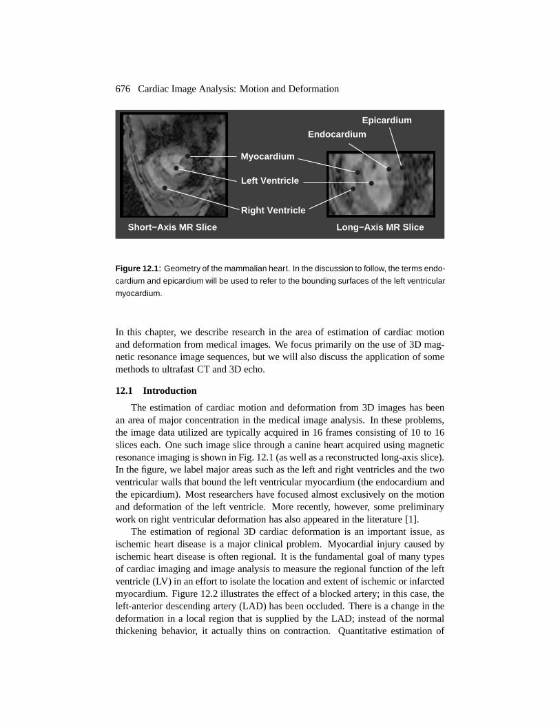
Figure 12.1: Geometry of the mammalian heart. In the discussion to follow, the terms endo-

cardium and epicardium will be used to refer to the bounding surfaces of the left ventricular

myocardium.

In this chapter, we describe research in the area of estimation of cardiac motionand deformation from medical images. We focus primarily on the use of 3D mag-netic resonance image sequences, but we will also discuss the application of somemethods to ultrafast CT and 3D echo.

12.1 Introduction

The estimation of cardiac motion and deformation from 3D images has beenan area of major concentration in the medical image analysis. In these problems,the image data utilized are typically acquired in 16 frames consisting of 10 to 16slices each. One such image slice through a canine heart acquired using magneticresonance imaging is shown in Fig. 12.1 (as well as a reconstructed long-axis slice).In the figure, we label major areas such as the left and right ventricles and the twoventricular walls that bound the left ventricular myocardium (the endocardium andthe epicardium). Most researchers have focused almost exclusively on the motionand deformation of the left ventricle. More recently, however, some preliminarywork on right ventricular deformation has also appeared in the literature [1].

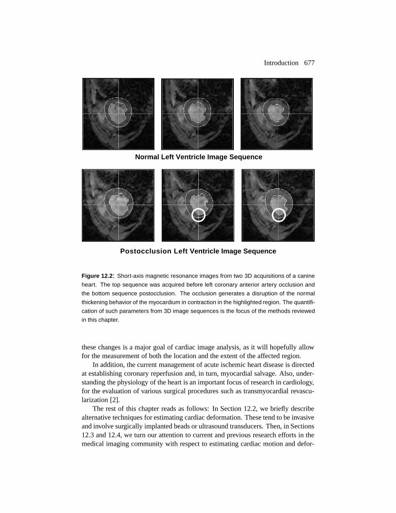
The estimation of regional 3D cardiac deformation is an important issue, asischemic heart disease is a major clinical problem. Myocardial injury caused byischemic heart disease is often regional. It is the fundamental goal of many typesof cardiac imaging and image analysis to measure the regional function of the leftventricle (LV) in an effort to isolate the location and extent of ischemic or infarctedmyocardium. Figure 12.2 illustrates the effect of a blocked artery; in this case, theleft-anterior descending artery (LAD) has been occluded. There is a change in thedeformation in a local region that is supplied by the LAD; instead of the normalthickening behavior, it actually thins on contraction. Quantitative estimation of

Introduction 677

Normal Left Ventricle Image Sequence

Postocclusion Left Ventricle Image Sequence

Figure 12.2: Short-axis magnetic resonance images from two 3D acquisitions of a canine

heart. The top sequence was acquired before left coronary anterior artery occlusion and

the bottom sequence postocclusion. The occlusion generates a disruption of the normal

thickening behavior of the myocardium in contraction in the highlighted region. The quantifi-

cation of such parameters from 3D image sequences is the focus of the methods reviewed

in this chapter.

these changes is a major goal of cardiac image analysis, as it will hopefully allowfor the measurement of both the location and the extent of the affected region.

In addition, the current management of acute ischemic heart disease is directedat establishing coronary reperfusion and, in turn, myocardial salvage. Also, under-standing the physiology of the heart is an important focus of research in cardiology,for the evaluation of various surgical procedures such as transmyocardial revascu-larization [2].

The rest of this chapter reads as follows: In Section 12.2, we briefly describealternative techniques for estimating cardiac deformation. These tend to be invasiveand involve surgically implanted beads or ultrasound transducers. Then, in Sections12.3 and 12.4, we turn our attention to current and previous research efforts in themedical imaging community with respect to estimating cardiac motion and defor-


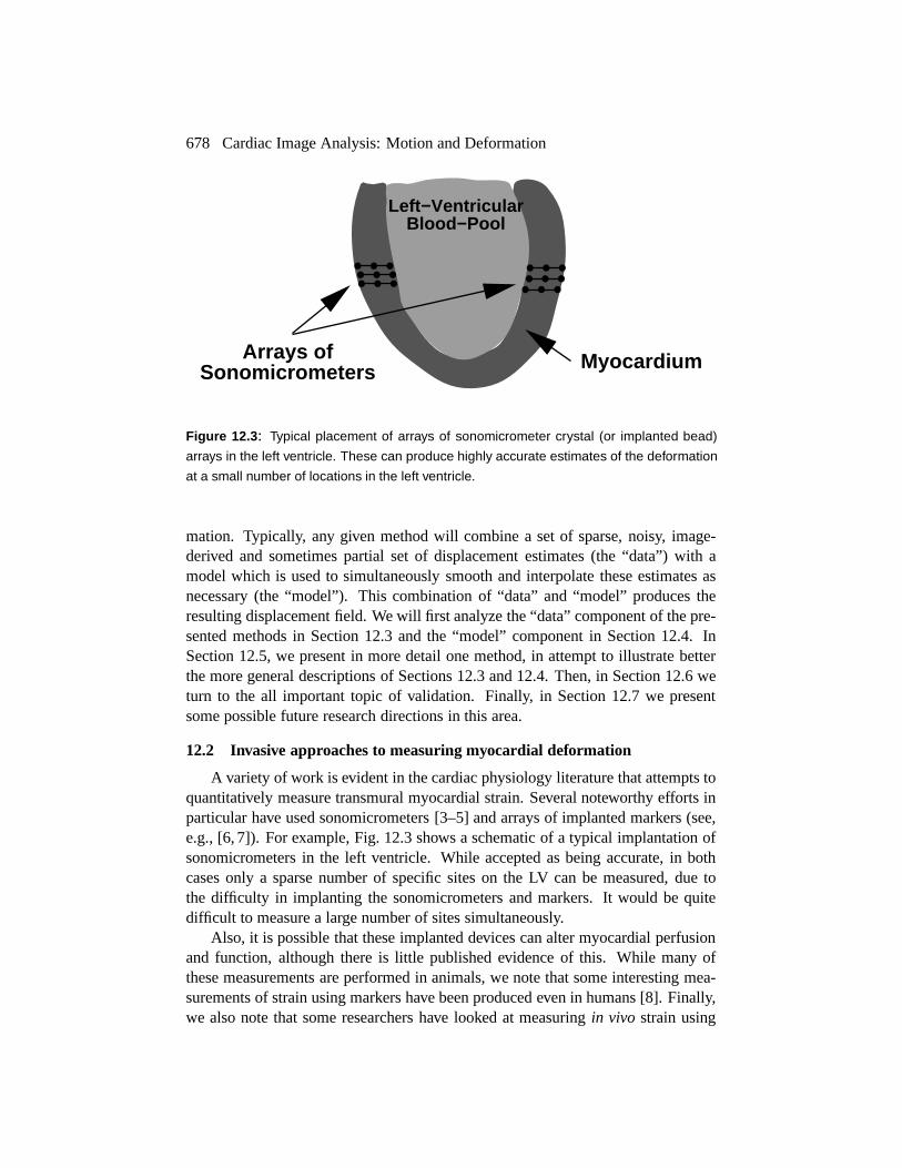
Arrays ofSonomicrometers Myocardium

Left−VentricularBlood−Pool

Figure 12.3: Typical placement of arrays of sonomicrometer crystal (or implanted bead)

arrays in the left ventricle. These can produce highly accurate estimates of the deformation

at a small number of locations in the left ventricle.

mation. Typically, any given method will combine a set of sparse, noisy, image-derived and sometimes partial set of displacement estimates (the “data”) with amodel which is used to simultaneously smooth and interpolate these estimates asnecessary (the “model”). This combination of “data” and “model” produces theresulting displacement field. We will first analyze the “data” component of the pre-sented methods in Section 12.3 and the “model” component in Section 12.4. InSection 12.5, we present in more detail one method, in attempt to illustrate betterthe more general descriptions of Sections 12.3 and 12.4. Then, in Section 12.6 weturn to the all important topic of validation. Finally, in Section 12.7 we presentsome possible future research directions in this area.

12.2 Invasive approaches to measuring myocardial deformation

A variety of work is evident in the cardiac physiology literature that attempts toquantitatively measure transmural myocardial strain. Several noteworthy efforts inparticular have used sonomicrometers [3–5] and arrays of implanted markers (see,e.g., [6, 7]). For example, Fig. 12.3 shows a schematic of a typical implantation ofsonomicrometers in the left ventricle. While accepted as being accurate, in bothcases only a sparse number of specific sites on the LV can be measured, due tothe difficulty in implanting the sonomicrometers and markers. It would be quitedifficult to measure a large number of sites simultaneously.

Also, it is possible that these implanted devices can alter myocardial perfusionand function, although there is little published evidence of this. While many ofthese measurements are performed in animals, we note that some interesting mea-surements of strain using markers have been produced even in humans [8]. Finally,we also note that some researchers have looked at measuring in vivo strain using

Approaches to obtaining estimates of cardiac deformation from 4D images 679

attached strain gauges [9] (as noted in [10]), although little has been pursued alongthese lines.

12.3 Approaches to obtaining estimates of cardiac deformation from 4D im-ages

There are two aspects to this problem; the first relates to the manipulation ofthe acquisition parameters in order to obtain the most-useful images, and the sec-ond to the postprocessing of these images for estimation of cardiac deformation.Regarding the first aspect, a significant level of activity has been performed withinthe magnetic resonance imaging (MRI) community regarding the development ofMR tagging, and to a lesser extent, MR phase velocity imaging. The underlyingphysics of these techniques is beyond the scope of this chapter; the interested readeris referred to a review article by Leon Axel [11].

The second aspect of this problem, the analysis of the images, relates to worktraditionally done in the computer vision community, especially in the areas of non-rigid motion estimation, including the case of variable illumination, segmentation,and surface mapping. A general, although somewhat dated coverage of the fieldcan be found in Horn [12].

In this section, we focus on the image-derived characteristics used to obtain theinitial, somewhat sparse, often noisy and partial displacements and/or velocitiesthat are combined with a model to produce complete and dense displacement anddeformation estimates.

12.3.1 Methods relying on magnetic resonance tagging

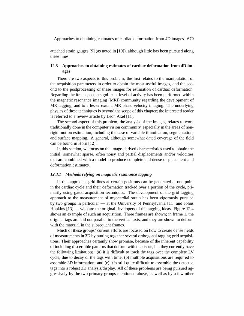
In this approach, grid lines at certain positions can be generated at one pointin the cardiac cycle and their deformation tracked over a portion of the cycle, pri-marily using gated acquisition techniques. The development of the grid taggingapproach to the measurement of myocardial strain has been vigorously pursuedby two groups in particular — at the University of Pennsylvania [11] and JohnsHopkins [13] — who are the original developers of the tagging ideas. Figure 12.4shows an example of such an acquisition. Three frames are shown; in frame 1, theoriginal tags are laid out parallel to the vertical axis, and they are shown to deformwith the material in the subsequent frames.

Much of these groups’ current efforts are focused on how to create dense fieldsof measurements in 3D by putting together several orthogonal tagging grid acquisi-tions. Their approaches certainly show promise, because of the inherent capabilityof including discernible patterns that deform with the tissue, but they currently havethe following limitations: (a) it is difficult to track the tags over the complete LVcycle, due to decay of the tags with time; (b) multiple acquisitions are required toassemble 3D information; and (c) it is still quite difficult to assemble the detectedtags into a robust 3D analysis/display. All of these problems are being pursued ag-gressively by the two primary groups mentioned above, as well as by a few other


Figure 12.4: Samples of short-axis (top) and long-axis (bottom) magnetic resonance im-

ages illustrating magnetic resonance tagging at three time points in the cardiac cycle. Cour-

tesy of Jerry L. Prince, John Hopkins University.

institutions (e.g. [14]).In general, there seem to be three different approaches to estimating initial dis-

placement data from magnetic resonance tagging as follows:

� Tagging in multiple intersecting planes and using the tag intersections astokens for tracking (e.g. [14–16]).

� Tagging in multiple intersecting planes, and then for each tagging plane es-timating the normal direction of motion perpendicular to the plane. Thisgenerates a sense of partial displacements (i.e., the component parallel to thetag lines is missing) to be combined later (e.g. [1, 17]).

� Attempting to model the tag fading over time using a model for the Blochequations and using a variable-brightness optical flow approach to extractthe displacements (e.g. [18, 19]).


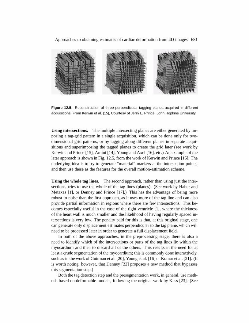
Figure 12.5: Reconstruction of three perpendicular tagging planes acquired in different

acquisitions. From Kerwin et al. [15], Courtesy of Jerry L. Prince, John Hopkins University.

Using intersections. The multiple intersecting planes are either generated by im-posing a tag-grid pattern in a single acquisition, which can be done only for two-dimensional grid patterns, or by tagging along different planes in separate acqui-sitions and superimposing the tagged planes to create the grid later (see work byKerwin and Prince [15], Amini [14], Young and Axel [16], etc.) An example of thelater approach is shown in Fig. 12.5, from the work of Kerwin and Prince [15]. Theunderlying idea is to try to generate “material”-markers at the intersection points,and then use these as the features for the overall motion-estimation scheme.

Using the whole tag lines. The second approach, rather than using just the inter-sections, tries to use the whole of the tag lines (planes). (See work by Haber andMetaxas [1], or Denney and Prince [17].) This has the advantage of being morerobust to noise than the first approach, as it uses more of the tag line and can alsoprovide partial information in regions where there are few intersections. This be-comes especially useful in the case of the right ventricle [1], where the thicknessof the heart wall is much smaller and the likelihood of having regularly spaced in-tersections is very low. The penalty paid for this is that, at this original stage, onecan generate only displacement estimates perpendicular to the tag plane, which willneed to be processed later in order to generate a full displacement field.

In both of the above approaches, in the preprocessing stage, there is also aneed to identify which of the intersections or parts of the tag lines lie within themyocardium and then to discard all of the others. This results in the need for atleast a crude segmentation of the myocardium; this is commonly done interactively,such as in the work of Guttman et al. [20], Young et al. [16] or Kumar et al. [21]. (Itis worth noting, however, that Denney [22] proposes a new method that bypassesthis segmentation step.)

Both the tag detection step and the presegmentation work, in general, use meth-ods based on deformable models, following the original work by Kass [23]. (See


Figure 12.6: An example of a low-frequency tagged MRI image. From Thetokis and Prince

[26]. Courtesy of Jerry L. Prince, John Hopkins University.

also chapter 3 and the review article by McInerney and Terzopoulos [24].) A de-formable model tries to find the curve that minimizes an energy functional thatconsists of an image-based term (typically the gradient) and an internal energy orsmoothness term. In the formulation of [23], it had the form�� !�� "�#� �%$ �'&(�� !�� "� � � � $ �"� �

(12.1)

where��

is the image as a function of the coordinates ��

;�

is the arclengththat parameterizes the curve; and

�and

&are the smoothing parameters. The

gradient term ensures adherence to the image data, whereas the second term tries tokeep the curve smooth. This approach is modified to allow for different deformablemodel geometries, such as grids [21], and for better image adherence terms usingsome knowledge of the underlying physics, such as in the case of [25].

Variable-brightness optical flow methods. In the third case, the whole imageis used, and data are extracted using a variable-brightness optical flow approachon the image intensity. Sinusoidal tagging patterns are primarily used in this case,which provide for the smooth intensity fields needed for efficient optical flow com-putation. See Fig. 12.6 for an example of this.

The variable-brightness part of the algorithm is based on modeling the fadingof the tag intensity over time using a model of the imaging process as generated bythe Bloch equations [18, 19]. For example, in the work of Gupta [19], the signal(brightness) at time ) is modeled as


� � ) �� "!#�$� �%�� &'��)(*�+�,��-��.� �(12.2)

where�/�

is the proton density, 0 ( and 0 � are the relation time constants, 021 is therepetition time, 043 is the echo time, and

!is the tag modulation coefficient. The

first three parameters (� � �

0 (�0 � ) are properties of the underlying tissue, whereas

the last three ( 0 1�053

�.!) are the acquisition parameters. In [19], a composite of the

tissue parameters is estimated as part of the displacement estimation algorithm.As with all intensity-based methods, the original estimates of the displacement

field consist of the component of the displacements perpendicular to the isophotes,(this limitation is known as the aperture problem; see Horn [12] for details) whichare later regularized to produce a full displacement estimate. The quality of theseestimates are highest in the middle of the wall and can be very noisy near themyocardial boundaries. This method has the advantage of not having to detect tagsexplicitly, but here the brightness variation parameters must be either known orestimated. A rough presegmentation of the ventricle is also needed here, to avoidsmoothing across the boundaries. These methods have, to the best knowledge ofthe authors, been applied only in 2D.

12.3.2 Methods relying on phase contrast MRI

Several investigators have employed changes in phase due to motion of tissuewithin a fixed voxel or volume of interest to assist in estimating instantaneous,localized velocities, and ultimately cardiac motion and deformation. While the ba-sic ideas were first suggested by van Dijk [27] and Nayler [28], it was Pelc andhis team [29–31] who first bridged the technique to conventional cine MR imag-ing and permitted the tracking of myocardial motion throughout the cardiac cycle.This technique relies basically on the fact that a uniform motion of tissue in thepresence of a magnetic field gradient produces a change in the MR signal phasethat is proportional to velocity. In principle, these instantaneous Eulerian velocitiescan be derived from each pixel in an image acquisition. An example of such anacquisition is shown in Fig. 12.7.

However, clusters of pixels within regions of interest (ROIs) are typically an-alyzed when predicting point-wise motion, primarily due to signal-to-noise issues.It is worth noting that, as with MR tagging, accurately tracking myocardial mo-tion in 3D requires additional image processing, and little has been reported in theliterature about this problem. Assembling the dense field phase velocity informa-tion into a complete and accurate 3D myocardial deformation map is currently alimiting problem for this technology. Furthermore, current phase-contrast velocityestimates near the endocardial and epicardial boundaries are less accurate. This isdue to the fact that the required size of an ROI — for signal-to-noise purposes —is typically large and can include information from outside the myocardial wall.


Thus, as with MR tagging, the most accurate LV function information is obtainedfrom the middle of the myocardial wall, and the least accurate information is usu-ally near the endocardial and epicardial wall boundaries. In general, there seemto be the following two common approaches to extracting useful information fromphase-contrast images:

� Processing the data directly to estimate strain rate tensors, e.g., [29, 32].

� Integrating the velocities over time, via some form of tracking mechanism toestimate displacements e.g., [33–36].

We also note that Shi [37] combined the phase-contrast velocities with shape-based displacements [38] within an integrated framework that is based on contin-uum mechanics.

12.3.3 Computer-vision-based methods

Quantifying the deformation of the LV can be seen as a two-step process: first,establish correspondence between certain points on the LV at time ) and time ) �+�

;and second, using these correspondences as a guide, solve for a complete mapping(embedding) of the LV between any two time frames. This problem can be posedfor the entire myocardium or just portions of it, such as the endocardial surfacealone. There has been considerable effort, in general, on these two topics, althoughrarely have they been addressed together.

One common approach to establishing correspondence is to track shaperelatedfeatures on the LV over time as reported by Goldgof [39], Ayache [40], McEachen[41], and Shi [38]. An example of such an approach in 2D is shown in Fig. 12.8.The preliminary displacement estimates here are, in general, generated using thefollowing steps:

� Extract the endocardial and epicardial surfaces from the images.

� Calculate the quantity that is used as the shape feature from these surfaces.These tend to be the curvatures; either the principal curvatures as in [38] orthe Gaussian curvature [39].

� Track points on the surfaces from one frame to the next by minimizing ametric such as bending energy or difference in curvature.

Then, the displacement field is smoothed (as was the case with previous meth-ods) to produce the final output displacements. A validation study of shape-basedtracking by comparing trajectories with implanted markers was reported by Shiet al. in [38], who found that the accuracy of tracking was within the resolutionof the image voxel sizes. Another interesting approach by Tagare [42] poses themapping problem in 2D as a bimorphism between two curves, thus eliminating thebasic asymmetry in the tracking process. This has not been extended to 3D yet.


Figure 12.7: One slice from a volumetric dataset obtained using magnetic resonance phase

contrast. The magnitude image is shown in the top left image. The other images show the

magnitudes of the velocity in the X, Y, and Z directions, respectively.

In general, all of the methods here depend on an accurate segmentation of theLV walls, but have the advantage of being imaging modality independent. Theyhave been used on MR, CT [38], and 3D ultrasound [43]. The dependency onobtaining an accurate segmentation, however, remains a significant issue, as therestill are no fully automated robust and efficient LV surface segmentation methods.The accuracy of the LV segmentation needed for these methods to be successful isobviously greater than in the case of methods using MR tagging. This is becausethe surfaces themselves provide the features, as opposed to being bounding sur-faces within which to search for intersections. We will examine a shape-trackingapproach in more detail, in the case study in Section 12.5.

There has been some work done on using the intensity of the images directly


Figure 12.8: Example of the shape-tracking approach. The goal is to map the original

surface to the final surface. For a point ��

on the original surface, a window � of plausible

matching points on the final surface is generated. Then, the point ��

in � that has the

most similar shape properties to ��

is selected as the candidate match point. The distance

function for shape similarity is typically based on the curvature(s).

to track the LV. Song and Leahy [44] used the intensity in ultrafast CT images tocalculate the displacement fields for a beating heart. This is similar in scope to someof the work done with MR tagging (e.g., [19]), but it does not have the advantageof a specially modulated image.

12.4 Modeling used for interpolation and smoothing

In general, the initial displacement fields produced by the methods discussed inthe previous section have the following characteristics:

� They are sparse. Displacements and/or velocities are only available at certainpoints and not for the whole of the myocardium.

� They are noise corrupted. This is an inherent problem in all medical imageanalysis methods, although the level of noise is very method dependent.

� They may be partial. Even where displacements and/or velocities are avail-able, only a certain component of the displacement vector may be known.

The estimation of accurate myocardial deformation requires a dense, smooth,and complete displacement field. This is because the deformation is typically cap-tured in terms of the strain that is a function of the derivatives of the displacement

Modeling used for interpolation and smoothing 687

field. The process of taking derivatives is very noise sensitive, and this is whatmakes this problem so challenging as compared to simply estimating the volumeof the LV which is an integral measure and hence relatively less sensitive to noise.

The interpolation and smoothing of the displacement field has been attackedin a number of ways. This step essentially constitutes the modeling step, and itis data-independent. The models contain implicitly or explicitly the assumptionsmade about the displacement field. All of the “models” currently used in this areaare passive; they ignore the fact that the heart is an actively contracting organ andnot a passive lump of tissue. Some of the modeling strategies are

� Impose a regularization constraint that penalizes the spatial derivatives, eitherexplicitly, as in [17, 19, 45], or combined in some cases with an isochoricconstraint1 [17,44]. This is further developed in the use of explicit continuummechanics models, which behave as regularizers, as in [1, 38, 46].

� Model the displacement field by using a smooth spatial parameterizationsuch as affine [33, 47] or splines [14, 15]. This method is used most oftenwhen displacement field modeling and tag extraction are combined in a sin-gle step, and is driven by the ease of parameterizing the geometry.

� Use of temporal smoothness or damping [1, 37, 42, 48] and temporal period-icity constraints [41].

In a sense, all of the above methods try to penalize the derivatives of the dis-placement, either in space, time, or both. We note that imposing a polynomialdistribution such as an affine model is equivalent to setting all derivatives higherthan a certain order to zero. This is a limiting case of penalizing spatial derivatives.

Spatial smoothness constraints. The application of spatial smoothness con-straints relies on the intuition that given that the myocardium is a single object,its displacement field can be expected to be smooth. If this is violated, then thetissue would tear apart. Therefore, high values of derivatives in the displacementfield (or equivalently high frequency components of its Fourier transform in thespatial sense) are likely to be the result of noise. This results in methods that pe-nalize the spatial derivatives, as in the optical flow method proposed by Horn andSchunk [49]. In this case, the optimal displacement field is found as a trade-offbetween satisfying the gradient constraint equation and a regularization term asfollows:

�� ) � �� (12.3)

1The myocardium is considered to be nearly incompressible and the isochoric constraint tries toenforce this incompressibility.


where the � is the displacement vector field over a space

that can be two- orthree-dimensional, ) is time, and

�represents the image.

The gradient constraint term� � & � � � �� essentially tries to match points of

equal intensity and is the data term, whereas the sum of squared derivatives multi-plied by the smoothness factor

�constitutes the regularizing term. The regularizing

term can be thought of as a model term, as it contains no image-related information.It captures the authors’ prior belief in the properties of the displacement field.

This framework is used in many of the approaches described earlier, althoughit is adapted to either match the data or the prior information. For example, in thecase of the variable-brightness optical flow method [18,19], the gradient constraintterm is replaced by a different measure that allows for the fading in the tag pattern.In a more general case, the gradient constraint term can be replaced by an image-data adherence term. This term tries to find a displacement field that stays close tosome pre-existing displacement estimates obtained by using approaches describedin Section 12.3. For example, if an estimate � �

of the displacement field exists, wecould modify the Horn and Schunk framework as follows:

��

� � �� (12.4)

We can expand on this model by also using an isochoric constraint that tries topenalize volume changes, as was done in [17,44]. This takes the form

� � � � � � and ismotivated by the fact that the myocardium — like most soft tissue — is thought tobe approximately incompressible2 . Alternatives also include the use of thin-splineenergy terms [15] or b-spline terms [14].

The combination of the smoothness and isochoric terms describes the my-ocardium in terms of what is essentially an internal energy function. Continuummechanics models of the myocardium as found in the biomechanics literature [50]are also described as internal energy functions, which also essentially penalizederivatives. So, it is a natural step at this point to try to bring some of this know-ledge into the inverse problem of motion estimation. To do this, the regulariza-tion term is replaced by an explicit mechanical model, which in most cases is anisotropic linear elastic [1, 37, 48] and in the case study we will consider it as trans-versely isotropic. This allows for us to account for the preferential stiffness of themyocardium along the fiber directions. It is interesting to note that, from contin-uum mechanics theory [51], an internal energy function can describe a real materialif and only if it is invariant to rigid translation and rotation; otherwise, this mate-rial violates the second law of thermodynamics. It can be shown that the classicalmodel of Horn and Schunk is not invariant to rotation and would fail this criterion.This is derived in the Appendix.

2There is in fact some change in volume, due to blood flow (reperfusion) into the wall, but this isconsidered to be small.

Modeling used for interpolation and smoothing 689

If we discretize Eq. (12.4), differentiate it with respect to � , and concatenate allthe individual displacements � into a large vector

�, we can write the generalized

expression:

� �� (12.5)

where�

is the assembled matrix of local derivative operators (as in [23]) andis sparse. This contains the model constraints that can be derived either from aregularization term or an explicit continuum mechanics model.

�is the external

driving force that tries to deform the model to adhere to the image data. Thisequation is most easily solved using the finite element method [52] , in cases ofcomplex geometry and especially in three dimensions.

Temporal smoothness constraints. There are two types of temporal smoothnessconstraints in the literature. In the first case, we have an explicit temporal filteringscheme applied to individual displacements. This is primarily, but not exclusively,done in the case where the input data is derived from phase contrast velocity. In thework of Meyer [33], a Kalman-filtering approach is used to smooth the displace-ment field. Zhu [35] and McEachen [41] parameterize the problem in the frequencydomain by expanding the displacement of an individual point over time in terms ofFourier series and try to take advantage of the periodicity of the left-ventricularmotion.

The second case involves extending Eq. (12.5) to include dynamics. This re-sults in the following generalized expression:

�� (12.6)

where�

is a mass matrix and

is a damping matrix. This approach also resultsin a form of temporal smoothing, which is motivated by similar approaches in con-tinuum mechanics. In the work of Park et al. [48], this was reduced to

��

by ignoring the mass matrix and setting the stiffness to 0. In [1], the stiffness termis also preserved. The full dynamical model is employed in Shi [37]; in this case,both shape-based displacements and phase-contrast velocity information are used.The full dynamical model is also used in work done in the computer vision andgraphics communities by Metaxas and Terzopoulos [53].

We note that Pentland [54] and Nastar [55] also use this approach and, by ig-noring the damping term, reduce it to a modal finite element equation, which pa-rameterizes the deformation in terms of the eigenmodes of the stiffness matrix

�.

In both of these approaches, however, there is no explicit notion of correspondencebetween material points, and the displacements are found using a global distancemeasure.


12.5 Case study: 3D cardiac deformation

In order to further clarify the more general statements of the previous sections,in this section we describe one approach to estimating the regional deformation ofthe left ventricle from magnetic resonance images. It has been previously reportedin [43, 46]. We use a biomechanical model to describe the myocardium and shape-based tracking displacement estimates on the epi- and endo cardial walls to generatethe initial displacement estimates. These are integrated in a Bayesian estimationframework, and the overall problem is solved using the finite element method. Thismethod produces quantitative regional 3D cardiac deformation estimates. We alsoshow results from 3D ultrasound data that illustrates the versatility of this approach.

12.5.1 Obtaining initial displacement data

In this work, we used both magnetic resonance and ultrasound images that wereacquired as follows:

MR images. ECG-gated magnetic resonance imaging was performed on a GESigna 1.5 Tesla scanner. Axial images through the LV were obtained with the gra-dient echo cine technique. The imaging parameters were section thickness = 5 mm,no intersection gap, 40 cm field of view, TE 13 msec, TR 28 msec, flip angle 30

�,

flow compensation in the slice and read gradient directions,��

��

matrix, and2 excitations. The resulting 3D image set consists of 16 2D image slices per tempo-ral frame, and 16 temporal 3D frames per cardiac cycle. The dogs were positionedin the magnetic resonance scanner for initial imaging under baseline conditions.The left anterior descending coronary artery was then occluded, creating an infarctregion where there was mechanical disfunction, and a second set of images wasacquired. An example of such an acquisition was shown in Fig. 12.2.

Ultrasound. The images were acquired using an HP Sonos 5500 Ultrasound Sys-tem with a 3D transducer (Transthoracic OmniPlane 21349A (R5012)). The 3Dprobe was placed at the apex of the left ventricle of an open-chest dog using asmall ultrasound gelpad (Aquaflex) as a standoff. Each acquisition consisted of13 to 17 frames per cardiac cycle depending on the heart rate. The angular slicespacing was 5

�, resulting in 36 image slices for each frame.

Image segmentation. The endo- and epicardial surfaces were extracted interac-tively using a software platform [56]. This platform was originally developed forMR image data and subsequently modified to allow for the different geometry andimage characteristics of ultrasound. For the automated part of the segmentation,we used an integrated deformable boundary method on a slice-by-slice basis. Theexternal energy function of the deformable contour consisted of the standard in-tensity term and, in the case of ultrasound images, a texture-based term similar to

Case study: 3D cardiac deformation 691

End−Diastole

End−Systole 3D wireframe in ima ge cards rendering

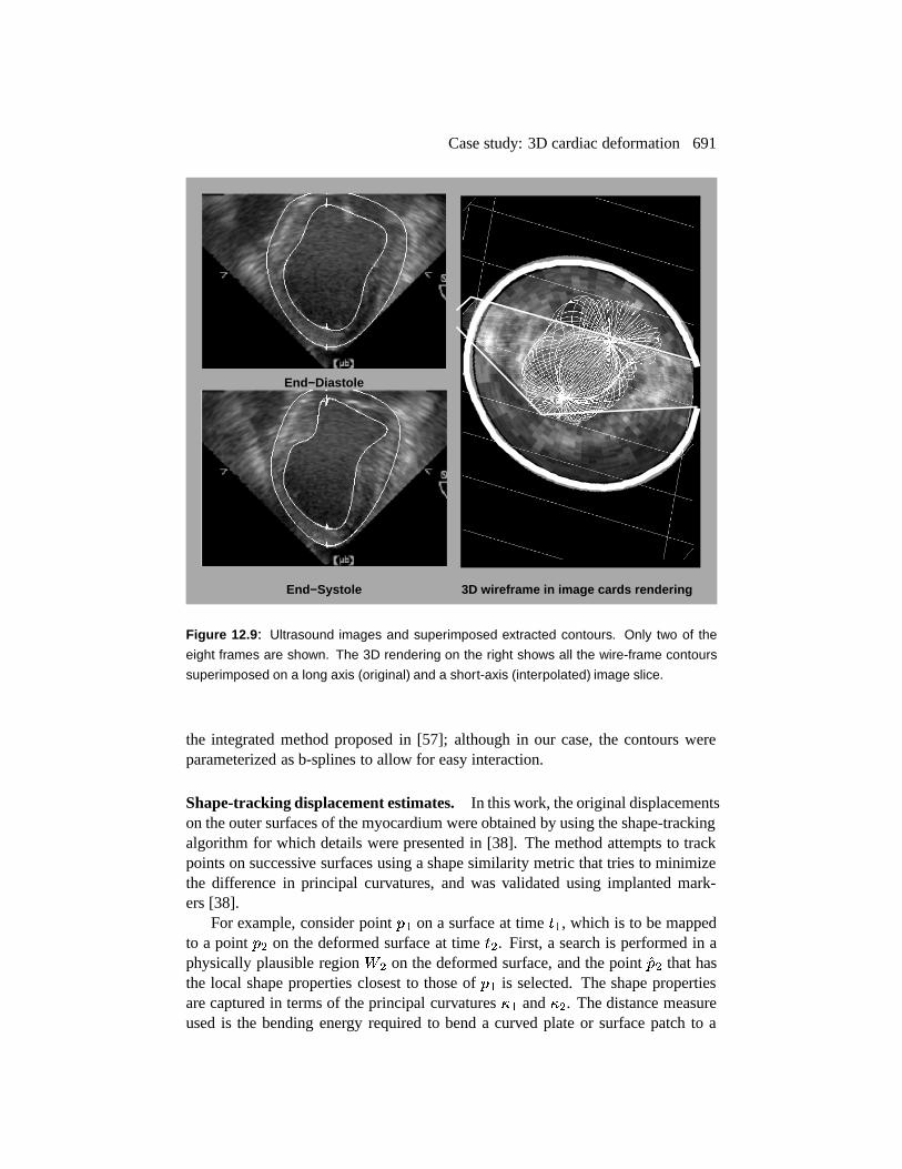
Figure 12.9: Ultrasound images and superimposed extracted contours. Only two of the

eight frames are shown. The 3D rendering on the right shows all the wire-frame contours

superimposed on a long axis (original) and a short-axis (interpolated) image slice.

the integrated method proposed in [57]; although in our case, the contours wereparameterized as b-splines to allow for easy interaction.

Shape-tracking displacement estimates. In this work, the original displacementson the outer surfaces of the myocardium were obtained by using the shape-trackingalgorithm for which details were presented in [38]. The method attempts to trackpoints on successive surfaces using a shape similarity metric that tries to minimizethe difference in principal curvatures, and was validated using implanted mark-ers [38].

For example, consider point � ( on a surface at time ) ( , which is to be mappedto a point � � on the deformed surface at time ) � . First, a search is performed in aphysically plausible region �

�on the deformed surface, and the point

�� that hasthe local shape properties closest to those of � ( is selected. The shape propertiesare captured in terms of the principal curvatures �

(and �

�. The distance measure

used is the bending energy required to bend a curved plate or surface patch to a


newly deformed state. This is labeled as� �� and is defined as� ��

� �� ( � � ( � � �

( � � � � � � � � � � � � ( �2� ��

� � � (12.7)

The displacement estimate vector for each point � ( , � � (is given by� � ( � �� ( ,

��

��

� ��

Confidence measures in the match. The bending energy measurement for all ofthe points inside the search region �

�are recorded as the basis for measuring the

strength and uniqueness of the matching choices. The value of the minimum bend-ing energy in the search region between the matched points indicates the goodnessof the match. Denoting this value as �� , we have the following measurement formatching goodness: �� ( � � � �� ( � �� (12.8)

On the other hand, it is desirable that the chosen matching point is a unique choiceamong the candidate points within the search window. Ideally, the bending energyvalue of the chosen point should be an outlier (much smaller value) compared tothe values of the rest of the points. If we denote the mean value of the bendingenergy measures of all the points inside window �

�except the chosen point as ��

and the standard deviation as �� , we define the uniqueness measure as�� ( �� ( � �� (12.9)

This uniqueness measure has a high value if the bending energy distance� �� to

the chosen point is large compared to some reference value (mean minus standarddeviation of the remaining bending energy measures). Combining these two mea-sures together, we arrive at one confidence measure � �

�� ( � for the matched point�� of point � ( :� �

�� ( �� (�� ( � � �� (�� ( � � (12.10)

where� (�� (�� , and

� � � � are scaling constants for normalization purposes.We normalize the confidences to lie in the range 0 to 1.

Modeling the initial displacement estimates. Given a set of displacement vectormeasurements � �

and confidence measures � �

, we model these estimates proba-bilistically by assuming that the noise in the individual measurements is normallydistributed with zero mean and a variance � � equal to

(�� . In addition, we assume


that the measurements are uncorrelated. Given these assumptions, we can write themeasurement probability for each point as

��

� � �*� ��

�� (12.11)

12.5.2 Modeling the myocardium

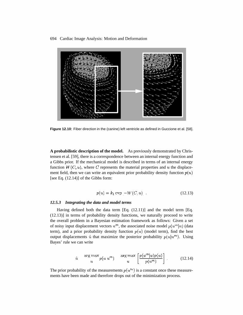
The passive properties of the left-ventricular myocardium are captured using abiomechanical model. We use an anisotropic linear elastic model, which allows usto incorporate information about the preferential stiffness of the tissue along fiberdirections from [58], which are shown in Fig. 12.10. The model is described interms of an internal or strain energy function.

Definition of strain. Consider a body �� , which after time ) moves and de-forms to body � ) � . A point X on �� goes to a point

on � ) � and the trans-

formation gradient�

is defined as� � � ��

. The deformation is expressed interms of the strain tensor � . Because the deformations to be estimated in this workare larger than 5%, we use a finite strain formulation implemented using a loga-rithmic strain �� , which is defined as � �� & . Since the strain tensor is a� ��

symmetric second-rank tensor (matrix), we can rewrite it in vector form as�#� � � (.( � �� ( � � ( �� & . This will enable us to express the tensor equations ina more familiar matrix notation.

Strain energy function. The mechanical model can be defined in terms of astrain energy function. The simplest useful continuum model in solid mechan-ics is the linear elastic one that is of the form �

� � � � � �"� � � & � � � � , where

is a� � �

matrix and defines the material properties of the deforming body, and� � � � is the strain vector that is a function of the displacement. The left ventricle ofthe heart is specifically modeled as a transversely elastic material to account for thepreferential stiffness in the fiber direction, by using this matrix

:

� �"!$#%&&&&&&&&'

!(*) �,+ )(-) �,+/. )( . 0 0 0�,+ )(*) !(-) �,+/. )( . 0 0 0�,+/. ) ( .( ) �,+/. ) ( .( ) !( . 0 0 00 0 0 1�2 !435+ )76( ) 0 00 0 0 0 !8 . 00 0 0 0 0 !8 .

9;::::::::<= (12.12)

where >@? is the fiber stiffness, >BA is cross-fiber stiffness, C-? A � CDA are the corre-sponding Poisson’s ratios, and EF? is the shear modulus across fibers. ( EG?IH> ?�J � � � � � CK? A �� ). If >@? � >�A and CLA � CK? A , this model reduces to the morecommon isotropic linear elastic model. The fiber stiffness was set to be

� � � timesgreater than the cross-fiber stiffness [58]. The Poisson’s ratios were both set to

� �NMto model approximate incompressibility.


Figure 12.10: Fiber direction in the (canine) left ventricle as defined in Guccione et al. [58].

A probabilistic description of the model. As previously demonstrated by Chris-tensen et al. [59], there is a correspondence between an internal energy function anda Gibbs prior. If the mechanical model is described in terms of an internal energyfunction �

� � � � , where

represents the material properties and � the displace-ment field, then we can write an equivalent prior probability density function �

� � �[see Eq. (12.14)] of the Gibbs form:

�� ( ��

� � � � � � (12.13)

12.5.3 Integrating the data and model terms

Having defined both the data term [Eq. (12.11)] and the model term [Eq.(12.13)] in terms of probability density functions, we naturally proceed to writethe overall problem in a Bayesian estimation framework as follows: Given a setof noisy input displacement vectors � �

, the associated noise model ��

� � � (dataterm), and a prior probability density function �

� � � (model term), find the bestoutput displacements

�� that maximize the posterior probability ��

�. Using

Bayes’ rule we can write

��

��

� � � ��

��

� � � (12.14)

The prior probability of the measurements ��

�is a constant once these measure-

ments have been made and therefore drops out of the minimization process.


Taking logarithms in Eq. (12.14) and differentiating with respect to the dis-placement field � results in a system of partial differential equations. When dis-cretized, this system of equations has the same form as Eq. (12.5), with the

�matrix being a function of the mechanical model and the geometry and

�a func-

tion of the data variances. This is solved using the finite element method [52]. Thefirst step in the finite element method is the division or tessellation of the body of in-terest into elements; these are commonly tetrahedral or hexahedral in shape. Oncethis is done, the partial differential equations are written down in integral form foreach element, and then the integral of these equations over all of the elements istaken to produce the final set of equations. For more information, one is referred totextbooks such as Bathe [52] . The final set of equations is then solved to producethe output set of displacements.

For each frame between end-systole (ES) and end-diastole (ED), a two-stepproblem is posed: (a) solving Eq. (12.14) and (b) using a modified nearest-neighbortechnique to map the position of all points on the endo- and epicardial surfacesso they lie on the endo- and epicardial surfaces at the next frame, and solvingEq. (12.14) once more using this added constraint. This ensures that there is nobias in the estimation of the radial strain.

12.5.4 Results

In this section, we present results from the application of this methodology onmultiple (16) sets of multiple time-frame sequences of in vivo left-ventricular MRimages. These consisted of eight canine experiments where images were acquiredbefore and after coronary occlusion. These will be referred to as the normal andpostocclusion studies. We also present some more preliminary results from threecanine experiments using ultrasound images. Of these, one was a normal study andthe other two were postocclusion studies.

In both cases, the images were segmented interactively using [56] and the sur-faces sampled to

� � � voxel resolution, at which point curvatures were calculated andthe shape-tracking algorithm was used to generate initial displacement estimates.The heart wall was divided into 1,000–2,000 hexahedral elements (depending onthe geometry), and the anisotropic linear elastic model was used to regularize thedisplacements. The computational time after the segmentation was on the order of2–4 hrs/dog (depending on the heart rate and hence the number of image frames)on a Silicon Graphics Octane with an R10000 195 MHz processor and 128 MBRAM.

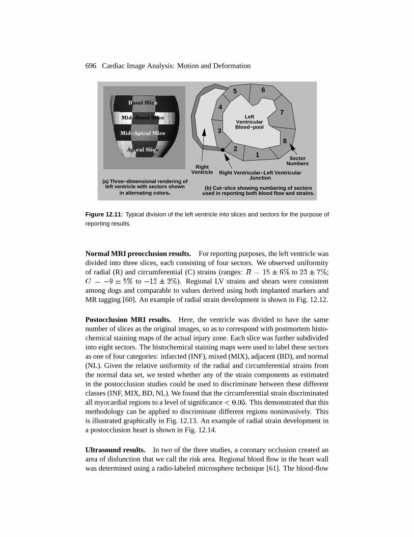
For the purpose of analyzing the results, the left ventricle of the heart wasdivided into a number of cross-sectional slices depending on its size and the postmortem information to which it was compared. Slice 1 was located at the bottomor apex of the ventricle. Each slice was further subdivided into 4 or 8 sectors; anexample is shown in Fig. 12.11.


(a) Three−dimension al rendering of left ventricle with sectors shown

in alternating colo rs .(b) Cut−slice showi ng numbering of sec tors

used in reporting b oth blood flow and strains .

Basal Slice

Apical Slice

Mid−Basal Slice

Mid−Apical Slice

12

3

4

5 6

7

8

RightVentricle

LeftVentricularBlood−pool

Right Ventricular −Left Ventricular Junction

SectorNumbers

Figure 12.11: Typical division of the left ventricle into slices and sectors for the purpose of

reporting results.

Normal MRI preocclusion results. For reporting purposes, the left ventricle wasdivided into three slices, each consisting of four sectors. We observed uniformityof radial (R) and circumferential (C) strains (ranges:

� � ��

to�K��

; � �� to

� ��

). Regional LV strains and shears were consistentamong dogs and comparable to values derived using both implanted markers andMR tagging [60]. An example of radial strain development is shown in Fig. 12.12.

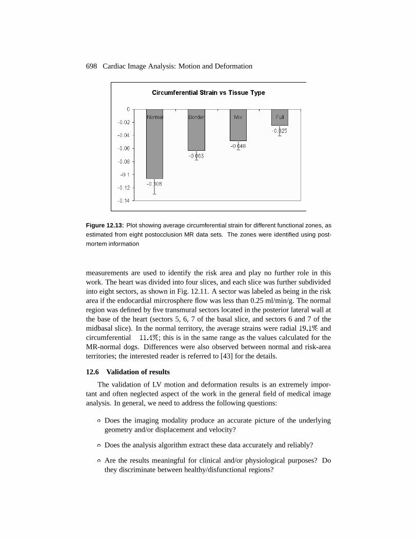
Postocclusion MRI results. Here, the ventricle was divided to have the samenumber of slices as the original images, so as to correspond with postmortem histo-chemical staining maps of the actual injury zone. Each slice was further subdividedinto eight sectors. The histochemical staining maps were used to label these sectorsas one of four categories: infarcted (INF), mixed (MIX), adjacent (BD), and normal(NL). Given the relative uniformity of the radial and circumferential strains fromthe normal data set, we tested whether any of the strain components as estimatedin the postocclusion studies could be used to discriminate between these differentclasses (INF, MIX, BD, NL). We found that the circumferential strain discriminatedall myocardial regions to a level of significance �

� � � � . This demonstrated that thismethodology can be applied to discriminate different regions noninvasively. Thisis illustrated graphically in Fig. 12.13. An example of radial strain development ina postocclusion heart is shown in Fig. 12.14.

Ultrasound results. In two of the three studies, a coronary occlusion created anarea of disfunction that we call the risk area. Regional blood flow in the heart wallwas determined using a radio-labeled microsphere technique [61]. The blood-flow


Frame 1 (ED) Frame 3

Frame 5 Frame 7

Frame 9 (ES)

Radial strain with respect��

�� 0% 30%

Scale: positive strain definedas thickening.

Figure 12.12: Radial strain development in a section of a normal left ventricle, as estimated

from MRI data. Normal behavior is exhibited, which is thickening (red). The strain pattern is

calculated throughout the left ventricle, but it is harder to visualize the full 3D picture, so a

2D cut is shown instead. (For a color version of this Figure see Plate 15 in the color section

of this book.)


Figure 12.13: Plot showing average circumferential strain for different functional zones, as

estimated from eight postocclusion MR data sets. The zones were identified using post-

mortem information

measurements are used to identify the risk area and play no further role in thiswork. The heart was divided into four slices, and each slice was further subdividedinto eight sectors, as shown in Fig. 12.11. A sector was labeled as being in the riskarea if the endocardial mircrosphere flow was less than 0.25 ml/min/g. The normalregion was defined by five transmural sectors located in the posterior lateral wall atthe base of the heart (sectors 5, 6, 7 of the basal slice, and sectors 6 and 7 of themidbasal slice). In the normal territory, the average strains were radial

� � � � � andcircumferential

� �� NM � ; this is in the same range as the values calculated for theMR-normal dogs. Differences were also observed between normal and risk-areaterritories; the interested reader is referred to [43] for the details.

12.6 Validation of results

The validation of LV motion and deformation results is an extremely impor-tant and often neglected aspect of the work in the general field of medical imageanalysis. In general, we need to address the following questions:

� Does the imaging modality produce an accurate picture of the underlyinggeometry and/or displacement and velocity?

� Does the analysis algorithm extract these data accurately and reliably?

� Are the results meaningful for clinical and/or physiological purposes? Dothey discriminate between healthy/disfunctional regions?

Validation of results 699

Frame 1 (ED) Frame 3

Frame 5 Frame 7

Frame 9 (ES)

Radial strain with respect��

�� 0% 30%

Scale: positive strain definedas thickening.

Figure 12.14: Radial strain development in a section of a postocclusion left ventricle, as

estimated from MRI data. Note the infarct region on the right colored as blue-green. Com-

pare the change from Fig. 12.12. (For a color version of this Figure see Plate 16 in the color

section of this book.)


End-Diastole End-Systole

0% 30%-30%

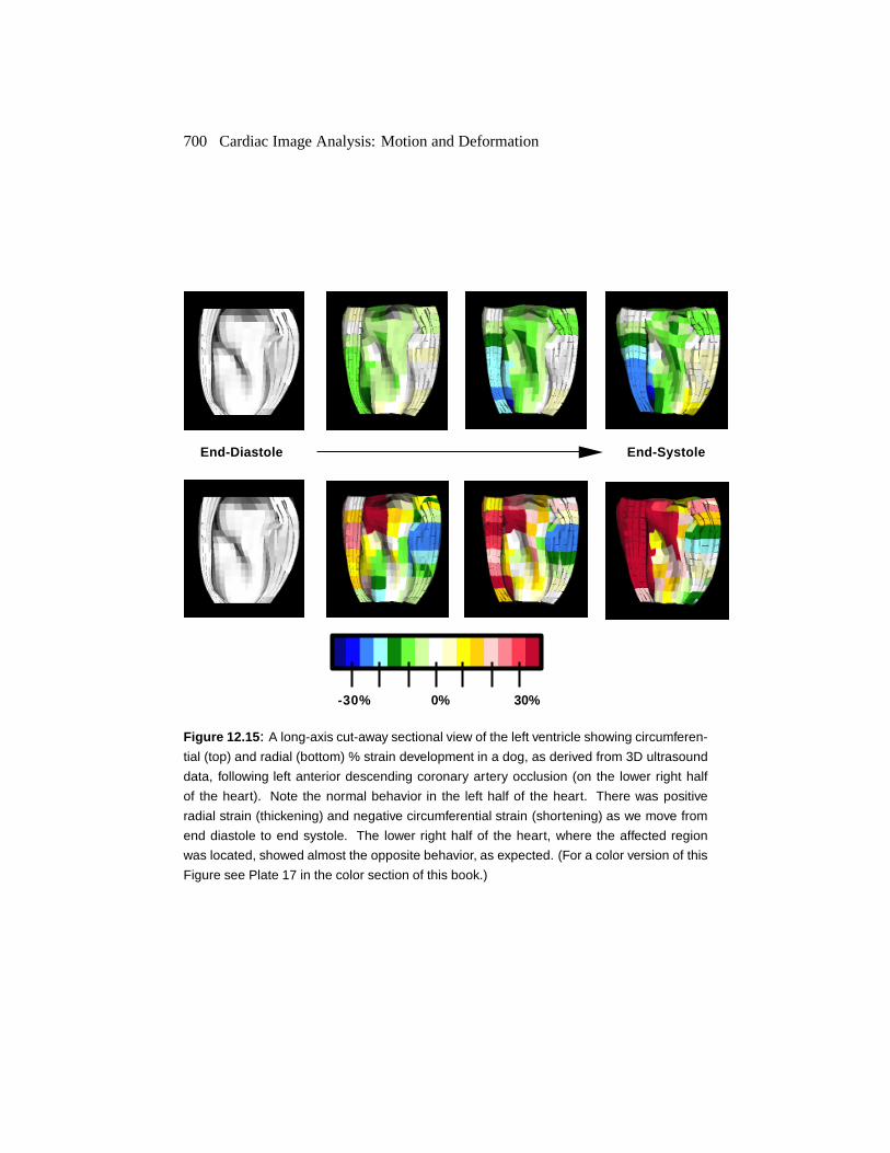
Figure 12.15: A long-axis cut-away sectional view of the left ventricle showing circumferen-

tial (top) and radial (bottom) % strain development in a dog, as derived from 3D ultrasound

data, following left anterior descending coronary artery occlusion (on the lower right half

of the heart). Note the normal behavior in the left half of the heart. There was positive

radial strain (thickening) and negative circumferential strain (shortening) as we move from

end diastole to end systole. The lower right half of the heart, where the affected region

was located, showed almost the opposite behavior, as expected. (For a color version of this

Figure see Plate 17 in the color section of this book.)

Validation of results 701

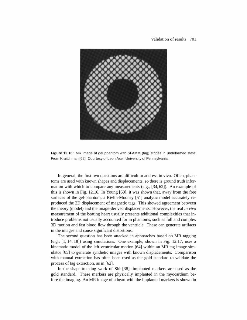
Figure 12.16: MR image of gel phantom with SPAMM (tag) stripes in undeformed state.

From Kraitchman [62]. Courtesy of Leon Axel, University of Pennsylvania.

In general, the first two questions are difficult to address in vivo. Often, phan-toms are used with known shapes and displacements, so there is ground truth infor-mation with which to compare any measurements (e.g., [34, 62]). An example ofthis is shown in Fig. 12.16. In Young [63], it was shown that, away from the freesurfaces of the gel-phantom, a Rivlin-Mooney [51] analytic model accurately re-produced the 2D displacement of magnetic tags. This showed agreement betweenthe theory (model) and the image-derived displacements. However, the real in vivomeasurement of the beating heart usually presents additional complexities that in-troduce problems not usually accounted for in phantoms, such as full and complex3D motion and fast blood flow through the ventricle. These can generate artifactsin the images and cause significant distortions.

The second question has been attacked in approaches based on MR tagging(e.g., [1, 14, 18]) using simulations. One example, shown in Fig. 12.17, uses akinematic model of the left ventricular motion [64] within an MR tag image sim-ulator [65] to generate synthetic images with known displacements. Comparisonwith manual extraction has often been used as the gold standard to validate theprocess of tag extraction, as in [62].

In the shape-tracking work of Shi [38], implanted markers are used as thegold standard. These markers are physically implanted in the myocardium be-fore the imaging. An MR image of a heart with the implanted markers is shown in


Figure 12.17: Example of the use of the cardiac simulator [64,65] used to validate methods

based on MR tagging. Left: the undeformed prolate spheroidal model of the LV in the

reference state. Right: a tagged image corresponding to a selected image plane. From

Amini [14]. Courtesy of Amir A. Amini, Washington University, St Louis.

Figure 12.18: 2D MR image slice of left ventricle with implanted markers used to validate

shape-based displacement estimates. From Shi [38].

Conclusions and further research directions 703

Fig. 12.18. This approach to validation tries to attack the first two questions simul-taneously. Here, algorithm-generated displacements are compared to the markerdisplacements (these are easily identifiable from the images). This technique hasthe disadvantage of comparing trajectories in a smaller number of points; however,it is done on real data, as opposed to simulations.

The third question is not addressed much in the image analysis literature, quan-titatively. Often, an example of the results on a normal and a hypertrophic heartis shown and the differences “correlated” with other evidence from the cardiologyliterature. It is known from both work reported in the case study in this chapter(see Section 12.5) and from the work of Croisille et al. [60], that, on average, thechanges between normal and abnormal regions in terms of radial and circumferen-tial strains is on the order of 10–15 %, and much smaller in the case of borderlineregions. A quick calculation shows that in the case of MR-tagging-based work,where the tags are typically 5 voxels apart at end-diastole, the change in the spac-ing at end-systole is going to be around 0.5 voxels or less. In the case of shape-based methods where the whole of the ventricle is used, this number is somewhatlarger (around 0.8 voxels). If such changes are to be detected reliably, and we wereto ignore accumulated tracking errors after the tags and/or boundaries have beenextracted, we need to be able to extract tags/boundaries at a precision of 0.25–0.4voxel or less. This is currently beyond the performance level of all automatic algo-rithms on real data; hence, manual and semiautomatic algorithms are used in mostcases. In both the case study and [60], the reported results are averaged over a num-ber of studies. This may be useful for exploring the physiology but not plausiblefor diagnosis, unless the results are averaged over large sections of the ventricle.

12.7 Conclusions and further research directions

The major problem/bottleneck in most of the work presented in this chapter isthe extraction of features such as tag lines and especially left ventricular surfacesfrom the image data. As mentioned in the previous section, there is a reliance onmanual and semiautomatic techniques to obtain this information. Another problem,which is less an issue of image analysis and more an issue of medical imagingtechnology, is the difficulty of using magnetic resonance in a clinical setting. It isnot possible to image patients in an emergency room (as is the case for examplewith ultrasound), and metallic objects such as pacemakers cause serious problemsand dangers when placed in the magnet.

As mentioned earlier, most of the models used to smooth and/or interpolate thedisplacement field are passive; they do not contain any active contraction informa-tion. This can result in an underestimation of the deformation, as the model biasesthe results toward no change. This was noted in the work of Park [48] and is thereason why no spatial smoothness was employed there. This, however, is not a suf-ficient solution to the problem, as some spatial smoothing is often needed to copewith the noise in the data and the sparseness in the image information. A possibly


better solution would be to incorporate some knowledge of the active contractionof the left ventricle during the first half of the cardiac cycle. This has the potentialof eliminating the bias problem, although it would introduce more parameters to beset or ideally estimated from the image data.

Magnetic resonance represents a promising modality and the development ofimproved analysis techniques will enhance the possibilities of it being used clin-ically. In the meantime we note that improvements in 3D echo technology, suchas the introduction of harmonic imaging [66] and contrast agents [67], are begin-ning to make this modality an attractive and somewhat cheaper alternative. Somepreliminary work has been reported in the case study (see also [43].) However, seg-menting ultrasound images is a very challenging problem whose solution will mostlikely require the use of temporal as well as spatial information. Some interestingfeature-extraction work was reported in [68].

12.8 Appendix A: Comparison of mechanical models to regularization

In this appendix, we explicitly compare the internal energy function generatedby isotropic linear elasticity with the equivalent energy function generated by theHorn and Schunk regularizer, as shown in Eq. (12.4).

Isotropic linear elasticity. The internal energy function generated by linear elas-ticity has the form:

�� & � �

(12.15)

where�

is the strain tensor written in vector form and

is the matrix of elasticproperties. (See also Section 12.5.2 in the case study.) In the case of infinitesimallinear elasticity, the strain tensor � is defined as

��

�

� � � ��

� � � � (12.16)

The strain is the symmetric component of the displacement to position Jaco-bian. Since it is a symmetric

� � �matrix, we can rewrite it in vector form as

�#� � � (.( � � �� ( � � � ( � � �7�� & � (12.17)

We can also define the complement tensor )�� )�� , which is the small rotationtensor, as the antisymmetric component of this Jacobian. Similarly, we write thisin vector form as

�� (.( � � �� ( � � � ( � � � �� & � (12.18)

References 705

The principle of material frame indifference [51] states that the internal energyfunction must be invariant to rigid translation and rotation. A sufficient conditionis that it must be a function of � and not a function of � .

Relation between regularization and linear elasticity. The internal energy func-tion used by Horn and Schunk can be rewritten as

��

�� & � � �

�� (12.19)

This is a function of the small rotation vector and hence does not satisfy theprinciple of material frame indifference. So this “mechanical” model is unreal-izable, which means that no material could exist with this strain energy function.This is because it contradicts the second law of thermodynamics, since the internalenergy function is not a function of the deformation alone but also a function ofthe rotation � . If the internal energy changes when a global rotation is applied, wearrive at the following problem: Suppose that work is needed to rotate the objectclockwise. From conservation principles, this energy will be returned when the ob-ject is turned counter-clockwise. We can keep turning the object counter-clockwiseto get more and more energy, and in this way we have created a perpetual motionmachine.

Therefore, one could define all realizable mechanical models as the subset ofregularization functionals that are invariant to global translation and rotation. View-ing the problem in this way does not make finding a model necessarily easier, butit does provide a way to eliminate inadmissible models.

12.9 References

[1] E. Haber, D. N. Metaxas, and L. Axel, “Motion analysis of the right ventricle fromMRI images,” in In Medical Image Computing and Computer-Assisted Intervention-MICCAI, (Cambridge, Mass.), October 1998.

[2] N. Gassler, H.-O. Wintzwer, H.-M. Stubbe, A. Wullbrand, and U. Helmchen, “Trans-myocardial laser revascularization: histological features in hyman nonresponder my-ocardium,” Circulation, pp. 371–5, 1997.

[3] K. Gallagher, G. Oksada, M. Miller, W. Kemper, and J. Ross, “Nonuniformity of innerand outer systolic wall thickening in conscious dogs,” Am J. Physiology, vol. 249,pp. H241–H248, 1985.

[4] T. Freeman, J. Cherry, and G. Klassen, “Transmural myocardial deformation in thecanine left ventricular wall,” Am J. Physiology, vol. 235, pp. H523–H530, 1978.

[5] D. P. Dione, P. Shi, W. Smith, P. D. Man, J. Soares, J. S. Duncan, and A. J. Sinusas,“Three-dimensional regional left ventricular deformation from digital sonomicrome-try,” in 19th Annual International Conference of the IEEE Engineering in Medicineand Biology Society, (Chicago, Ill.), pp. 848–851, March 1997.


[6] L. Waldman, Y. Fung, and J. Covell, “Transmural myocardial deformation in thecanine left ventricle,” Circ Res, vol. 57, pp. 152–163, 1985.

[7] G. D. Meier, M. Ziskin, W. P. Santamore, and A. Bove, “Kinematics of the beatingheart,” IEEE Trans Biomed Eng, vol. 27, pp. 319–329, 1980.

[8] N. Ingels, G. Daughters, E. Stinson, and E. Alderman, “Measurement of midwallmyocardial dynamics in intact man by radiography of surgically implanted markers,”Circulation, vol. 52, pp. 859–867, November 1975.

[9] J. M. Dieudonne, “Gradients de directions et la deformations principales dans la paroiventriculaire gauch normale,” J. Physiol. Paris, vol. 61, pp. 305–330, 1969.

[10] H. Azhari et al., “Noninvasive quantification of principal strains in normal caninehearts using tagged MRI images in 3D,” Am. J. Physiol., vol. 264, pp. H205–H216,1993.

[11] L. Axel, “Physics and technology of cardiovascular MR imaging,” Cardiology Clin-ics, vol. 16, no. 2, pp. 125–133, 1998.

[12] B. K. P. Horn, Robot Vision. New York: McGraw-Hill, 1986.

[13] E. R. McVeigh, “Regional myocardial function,” Cardiology Clinics, vol. 16, no. 2,pp. 189–206, 1998.

[14] A. A. Amini, Y. Chen, R. W. Curwen, V. Manu, and J. Sun, “Coupled b-snake gridesand constrained thin-plate splines for analysis of 2-D tissue defomations from taggedMRI,” IEEE Transactions on Medical Imaging, vol. 17, pp. 344–356, June 1998.

[15] W. S. Kerwin and J. L. Prince, “Cardiac material markers from tagged MR images,”Medical Image Analysis, vol. 2, no. 4, pp. 339–353, 1998.

[16] A. A. Young, D. L. Kraitchman, L. Dougherty, and L. Axel, “Tracking and finiteelement analysis of stripe deformation in magnetic resonance tagging,” IEEE Trans-actions on Medical Imaging, vol. 14, pp. 413–421, September 1995.

[17] T. S. Denney, Jr and J. L. Prince, “Reconstruction of 3-D Left Ventricular Motionfrom Planar Tagged Cardiac MR Images: An Estimation Theoretic Approach,” IEEETransactions on Medical Imaging, vol. 14, pp. 625–635, December 1995.

[18] J. L. Prince and E. R. McVeigh, “Motion estimation from tagged MR image se-quences,” IEEE Transactions on Medical Imaging, vol. 11, pp. 238–249, June 1992.

[19] S. N. Gupta and J. L. Prince, “On variable brightness optical flow for tagged MRI,”in Information Processing in Medical Imaging, June 1995.

[20] M. Guttman, J. Prince, and E. McVeigh, “Tag and contour detection in tagged MRimages of the left ventricle,” IEEE Transactions on Medical Imaging, vol. 13, no. 1,pp. 74–88, 1994.

[21] S. Kumar and D. Goldgof, “Automatic tracking of SPAMM grid and the estimation ofdeformation parameters from cardiac images,” IEEE Transactions on Medical Imag-ing, vol. 13, March 1994.

[22] T. S. Denney Jr, “Estimation and detection of myocardial tags in MR images withoutuser-defined myocardial contours,” IEEE Transactions on Medical Imaging, vol. 18,pp. 330–344, April 1999.

References 707

[23] M. Kass, A. Witkin, and D. Terzopoulos, “Snakes: Active contour models,” in Proc.Int. Conf. on Computer Vision, pp. 259–268, 1987.

[24] T. McInerney and D. Terzopoulos, “Deformable models in medical image analysis: asurvey,” Medical Image Analysis, vol. 1, no. 2, pp. 91–108, 1996.

[25] A. A. Amini, R. W. Curwen, R. T. Constable, and J. C. Gore, “MR physics-basedsnake tracking and dense deformations from tagged cardiac images,” in AAAI Int.Symp. Comp. Vision Med. Image Processing., 1994.

[26] S. Androutsellis-Theotokis and J. L. Prince, “Experiments in multiresolution motionestimation for multifrequency tagged cardiac MR images,” in Int. Conf. on ImageProcessing, (Lausanne, Switzerland), September 1996.

[27] P. van Dijk, “Direct cardiac NMR imaging of heart wall and blood flow velocity,” J.Comp. Assist. Tomog., vol. 8, pp. 429–436, 1984.

[28] G. Nayler, N. Firmin, and D. Longmore, “Blood flow imaging by cine magnetic res-onance,” J. Comp. Assist. Tomog., vol. 10, pp. 715–722, 1986.

[29] N. J. Pelc, “Myocardial motion analysis with phase contrast cine MRI,” in Proceed-ings of the 10th Annual SMRM, (San Francisco), p. 17, 1991.

[30] N. J. Pelc, R. Herfkens, and L. Pelc, “3D analysis of myocardial motion and defor-mation with phase contrast cine MRI,” in Proceedings of the 11th Annual SMRM,(Berlin), p. 18, 1992.

[31] N. Pelc, R. Herfkens, A. Shimakawa, and D. Enzmann, “Phase contrast cine magneticresonance imaging,” Magn. Res. Quart., vol. 7, no. 4, pp. 229–254, 1991.

[32] V. Wedeen, “Magnetic Resonance Imaging of Myocardial Kinematics: Techniqueto Detect, Localize and Quantify the Strain Rates of Active Human Myocardium,”Magn. Reson. Med., vol. 27, pp. 52–67, 1992.

[33] F. G. Meyer, R. T. Constable, A. J. Sinusas, and J. S. Duncan, “Tracking MyocardialDeformation Using Phase Contrast MR Velocity Fields: A Stochastic Approach,”IEEE Transactions on Medical Imaging, vol. 15, August 1996.

[34] T. Constable, K. Rath, A. Sinusas, and J. Gore, “Development and evaluation of track-ing algorithms for cardiac wall motion analysis using phase velocity MR imaging,”Magn. Reson. Med., vol. 32, pp. 33–42, 1994.

[35] Y. Zhu, M. Drangove, and N. J. Pelc, “Estimation of deformation gradient and strainfrom cine-pc velocity data,” IEEE Transactions on Medical Imaging, vol. 16, Decem-ber 1997.

[36] R. Herfkens, N. Pelc, L. Pelc, and J. Sayre, “Right ventricular strain measured byphase contrast MRI,” in Proceedings of the 10th Annual SMRM, (San Francisco),p. 163, 1991.

[37] P. Shi, A. J. Sinusas, R. T. Constable, and J. S. Duncan, “Volumetric DeformationAnalysis Using Mechanics-Based Data Fusion: Applications in Cardiac Motion Re-covery,” International Journal of Computer Vision, Kluwer, in-press.


[38] P. Shi, A. J. Sinusas, R. T. Constable, E. Ritman, and J. S. Duncan, “Point-trackedquantitative analysis of left ventricular motion from 3D image sequences,” IEEETransactions on Medical Imaging, in-press.

[39] C. Kambhamettu and D. Goldgof, “Curvature-based approach to point correspon-dence recovery in conformal nonrigid motion,” CVGIP: Image Understanding,vol. 60, pp. 26–43, July 1994.

[40] I. Cohen, N. Ayache, and P. Sulger, “Tracking points on deformable objects usingcurvature information,” in Lecture Notes in Computer Science-ECCV92, pp. 458–466, Springer Verlag, 1992.

[41] J. McEachen, A. Nehorai, and J. Duncan, “A recursive filter for temporal analysisof cardiac function,” in IEEE Workshop on Biomedical Image Analysis, (Seattle),pp. 124–133, June 1994.

[42] H. D. Tagare, “Shape-based nonrigid curve correspondence with application to heartmotion analysis,” IEEE Transactions on Medical Imaging, vol. 18, pp. 570–579, July1999.

[43] X. Papademetris, A. J. Sinusas, D. P. Dione, and J. Duncan, “3D cardiac deformationfrom ultrasound images,” in Medical Image Computing and Computer Aided Inter-vention (MICCAI), (Cambridge, England), pp. 420–429, September 1999.

[44] S. Song and R. Leahy, “Computation of 3D velocity fields from 3D cine CT images,”IEEE Transactions on Medical Imaging, vol. 10, pp. 295–306, Sept 1991.

[45] A. A. Young, “Model tags; direct 3D tracking of heart wall motion from tagged MRIimages,” in MICCAI, (Boston, Massachusetts), pp. 92–101, October 1998.

[46] X. Papademetris, P. Shi, D. P. Dione, A. J. Sinusas, and J. S. Duncan, “Recovery ofsoft tissue object deformation using biomechanical models,” in Information Process-ing in Medical Imaging, (Visegrad, Hungary), pp. 352–357, June 1999.

[47] W. Odell, C. Moore, and E. McVeigh, “Displacement field fitting approach to calcu-late 3D deformations from parallel tagged grids,” J. Mag. Res. Imag., vol. 3, p. P208,1993.

[48] J. Park, D. N. Metaxas, and L. Axel, “Analysis of left ventricular wall motion based onvolumetric deformable models and MRI-SPAMM,” Medical Image Analysis, vol. 1,no. 1, pp. 53–71, 1996.

[49] B. K. P. Horn and B. G. Schunk, “Determining optical flow,” Artificial Intelligence,vol. 17, pp. 185–203, 1981.

[50] P. J. Hunter, A. McCulloch, and P. Nielsen, eds., Theory of Heart. Berlin: Springer-Verlag, 1991.

[51] L. E. Malvern, Introduction to the Mechanics of a Continuous Medium. EnglewoodCliffs, New Jersey: Prentice-Hall, 1969.

[52] K. Bathe, Finite Element Procedures in Engineering Analysis. New Jersey: Prentice-Hall, 1982.

References 709

[53] D. Terzopoulos and D. Metaxas, “Dynamic 3D models with local and global de-formation: deformable superquadrics,” IEEE Transactions on Pattern Analysis andMachine Intelligence, vol. 13, no. 17, 1991.

[54] B. Horowitz and S. Pentland, “Recovery of non-rigid motion and structure,” inProceedings of the IEEE Conference on Computer Vision and Pattern Recognition,(Maui), pp. 325–330, June 1991.

[55] C. Nastar and N. Ayache, “Classification of nonrigid motion in 3D images usingphysics-based vibration analysis,” in Workshop on Biomedical Image Analysis, (Seat-tle, Washington), pp. 61–69, 1994.

[56] X. Papademetris, J. V. Rambo, D. P. Dione, A. J. Sinusas, and J. S. Duncan, “Visuallyinteractive cine-3D segmentation of cardiac MR images,” Suppl. to the J. Am. Coll.of Cardiology, vol. 31, February 1998.

[57] A. Chakraborty, M. Worring, and J. S. Duncan, “On multi-feature integration fordeformable boundary finding,” Proc. Int. Conf. on Computer Vision, pp. 846–851,1995.

[58] J. M. Guccione and A. D. McCulloch, “Finite element modeling of ventricular me-chanics,” in Theory of Heart (P. J. Hunter, A. McCulloch, and P. Nielsen, eds.),pp. 122–144, Berlin: Springer-Verlag, 1991.

[59] G. E. Christensen, R. D. Rabbitt, and M. I. Miller, “3D brain mapping using de-formable neuroanatomy,” Physics in Medicine and Biology, vol. 39, pp. 609–618,1994.

[60] P. Croissile, C. C. Moore, R. M. Judd., J. A. C. Lima, M. Arai, E. R. McVeigh, L. C.Becker, and E. A. Zerhouni, “Differentiation of viable and nonviable myocardium bythe use of three-dimensional tagged MRI in 2-day-old reperfused infarcts.,” Circula-tion, vol. 99, pp. 284–291, 1999.

[61] A. J. Sinusas, K. A. Trautman, J. D. Bergin, D. D. Watson, M. Ruiz, W. H. Smith,and G. A. Beller, “Quantification of area of risk during coronary occlusion and de-gree of myocardial salvage after reperfusion with technetium-99m methoxyisobutylisonitrile.,” Circulation, vol. 82, pp. 1424–37, 1990.

[62] D. L. Kraitchman, A. A. Young, C. C, and L. Axel, “Semi-automatic tracking ofmyocardial motion in MR tagged images,” IEEE Transactions on Medical Imaging,vol. 14, pp. 422–433, September 1995.

[63] A. A. Young, L. Axel, et al., “Validation of tagging with MR imaging to estimatematerial deformation,” Radiology, vol. 188, pp. 101–108, 1993.

[64] T. Arts, W. Hunter, A. Douglas, A. Muijtens, and R. Reneman, “Description of thedeformation of the left ventricle by a kinematic model,” J. Biomechanics, vol. 25,no. 10, pp. 1119–1127, 1992.

[65] E. Waks, J. L. Prince, and A. Douglas, “Cardiac motion simulator for tagged MRI,”in Mathematical Methods in Biomedical Imaging Analysis, pp. 182–191, 1996.

[66] K. Caidahl, E. Kazzam, J. Lingberg, G. N. Andersen, J. Nordanstig, S. R. Dahlqvist,A. Waldenstro, and R. Wikh, “New concept in echocardiography: harmonic imagingof tissue withoug use of contrast agent.,” The Lancet, vol. 352, pp. 1264–1270, 1999.


[67] T. R. Porter, F. Xie, A. Kricsfeld, A. Chiou, and A. Dabestani, “Improved endocardialborder resolution using dobutamin stress endocardiography with intravenous soni-cated dextrose albumin.,” J. Am College of Cardiology, vol. 23, pp. 1440–43, 1994.

[68] M. M.-P. Miguel and J. A. Noble, “2D+T acoustic boundary detection in echocardio-graphy,” in MICCAI, (Boston, Massachusetts), October 1998.

chapter 12 cardiac image analysis: motion and deformation

Documents