chapter 14 statistical models for the prediction …chapter 14 . statistical models for the...
TRANSCRIPT

CHAPTER 14
STATISTICAL MODELS FOR THE PREDICTION OF FIELD-SCALE AND
SPATIAL SALINITY PATTERNS FROM SOIL CONDUCTIVITY SURVEY DATA
S M Lesch
wllection of apparen t soil electrical conductivity Ca) survey data purpose of characterizing various spatially referenced soil propershy
R eived considerable attention in the soils literature over the last d Jdes (Corwin and Lesch 200Sab) Although now commonly used
mJOI precisi011 agriculture survey applications most of the original t l in ECsurvey data was motivated by the need to characterize and oil salinity in a cost-effective manner (Rhoades et a1 1999 H nshy
~ et al 2002) The need for such surveying work is exp ected to ll~~ over time as more agricultural land becomes degraded due to ~ilJtion
par nt soil conductivity survey data often correlat reasonably well til Iariolls soil properties (salinity soil texture soil water content etc) Jlr different field conditions (Corwin and Lesch 2005b Lesch and ~m 2003) However as a general rule EC survey readings tend to be n1~ correlated with soil salinity levels Thus accurate salinity p redicshy can normally be constructed from EC survey data in semi-saline a line fi elds using fairly simple statistical calibration techniques
JIIi mally accurate maps of the field-scale salinity pattern can someshyalso be produced from ECa survey data in marginally saline field
11ided that other important soil properties (such as soil texture and soil Jt~r content) exhibit fairly minimal spatial variation
461
462 AGRIC ULTU RAL SALI NI TY ASSESSMENT AND MA NAGEME T
After ECa surv y data have been acquired in a field calibratlln samples are normally collected a t a certain number f EC sun ( JI_ tions The measured salinity level associated with these soil sampll then used (in conjlmction with the co-located survey data) to e tim
some type of spatial-statistical or geostatistical model This 5 ti1tl~ti
mod I is in turn used to predict the detailed spa tia l soil-salinity pJtt fr m the full set of acquired survey data
This chapter d iscusses th simplest and most fr quently used tdh~tll mod ling approach for calibra ting ECa survey information with mt ured salinity data such as ordinary regression Ordinar y linear regrl I
models represent a special case of a much more general das of mild conunonly known a linear regression models with spatially COrrtIJa
rrors (Schabenberger and Gotway 2005) hierarchical spatial nlllJ (Banerjee et al 2004) or geostatistical mixed linear mod (Haskard tI 2007) This bro( del lass of models in cludes many of th geos ta tisth t chniques familiar to soil scientists such as universal krigin and Jn~r
with external d rift as well as standard regression techniqu s-ordmill linear regre sian (LR) models and analysis of covariance models
The rem aind er of this chapter is organized as follows A tcchni review of the basic linear regression model es timation and validati techniques is p resented in Regression Models and Regres ion Ml~l Validation Tests Some suitable sampling strategies for calibrating lin r regres i n equations are discussed in Sampling Stra tegies while 1M sub quen t section presents a brief overview of th ESAP software pacmiddot age Two alinity assessment examples are then presented in Da Analysis Examples these data analyses demonstrate the stabstical call b ration and prediction t chniques discu s d in this chapter along witl some of the types of analysis outpu t that the ESAP software can produ
Regression Models Estimation and Prediction Formulas
Site-specific p r diction of diverse soil properties from EM survev dal can be ach ieved using regression model estimation and pr diction tcchmiddot niques In the r gression modeling approach advoca ted by Lesch and Corwin (2008) Lesch (2005) Rhoades et a1 (1999) and Lesch et al (1911 a suitable linear equation is specified that relates the target soil prop rtI
of interest to a linear combination of conductivity signa l data readin~
and (possibly) trend smfac coordinates One example of sltch an equlshytion would be
where the response variable (y) represen ts the soil prope rty of inte rl~ t
(eg salinity texture water content) at the ith survey location the predicmiddot
s
If lflab
nd lOrll
t lrions 1Jd ( t - with wplrt J
hl1 U1rrc
i 111 n ll l
mndll il llL y
lik li hllr t el l I q
InW rei U~ d In nwcssil spatially
The Ii (I l ppo (I middotd to ~
llmJudi vh n tJ pLctaliz melle re
ltnn cnli Allh
1( on 1(lw ing I notation roll )wil 1 - X() mcnts (
imlCAL MO DELS FO TH E PREDICTION OF FIELD-SCALE 463
(EMlI EMil CX cy ) represen t the corresponding EM38 vertical Inta l signal readings and associated ith su rvey site coordinate relti pectively the (3 p arameters represent empirical regression lfilicnts and E represents the random error component asso ishythe modeJ Equation 14-1 relates the response variable (e g soil
II I both EJv[ signal and trend surface components and thus can 1~ a signal + trend model The tr n d surface components
i11 Eq 14-] are optional and should only be included if they are necessa ry (i e if the associated parameter estimates are statisshy
)oificant or if the inclusion o f such components is needed to nnbvious spatial trend in a residual plot)
tpt imal estimation of the aforementioned (or similar) regression Jlp~nds on the assumptions placed on the random error com poshy
rro rs ar assumed to be normally distributed and exhibi t spashydation then Eq 14-1 is commonly called a spatial linear regresshylid in the statis tical literature or a kriging with external drift r Ihe geosta tisticalli terature (Cressie 1991 Schab nberger and 21105) Such models can be efficiently estimated using maximum
or restricted m aximum likeLihood fi tt ing techniques (Littell f-JoJ In contrast if the errors can be assLUned to be approximately
then ordinary least squares (OLS) fitting techniques can be this latter ca e the model becomes identical to an ordinar linear
eq uation the only difference being that the predictions are referenced
~keli h(lod of the r sidual errors being approximately uneoa-ela ted I)lli to spatially corr lated) depends primarily on (1) the method
llect the calibration sa mple sites and (2) the degree to which the Ity signal data correla tes with the respons variable of interest
he ignal de ta is strongly corr lated with the targe t soil p roperty and IOIIIJld ampJing strategies a re employed th assump tion of approxishy
nidual independence is often satisfied Fo r detailed discussions these i ues see Lesch and Corwin (2008) and esch (2005)
huugh appropriate prediction statistics can be d rived for either Iflly the OLS results are presented here Additionally 11 of the folshyrlSults are pr sented in matrix nota tion a good review of matrix nirom a regre ion modeling viewpoint is given in Myers (1986) In~ standard matrix notation note that we can express Eq 14-1 as
d ~ e where y repre nts a (n x 1) vector of soil property measureshy(collected across n itls) X represents th e correspondin g (n x p) ion model de ign matrix and e represents the (n x 1) vector of
(I ~ 1 IlJ Ierrors Then under the LU1correlated residual error assumption tlinear unbiased estimate (BLU E) for (3 is
f in It r l pI di (14-2)
464 AGRICULTURAL SALINITY ASSESSMENT AND MANAGEvIENT
with a corresponding variance of
[1
where (J2 represents the regression model mean square error (MSEI( ponent
Likewise the residuals (ie empirical model errors) for Eq I-H defined to be
r = y - Xf3 ( I
and these residuals provide an unbiased estimate of the MSEcompon~l
that is
Now let Yzrepresent the (unknown) vector of soil property values at til the remaining survey locations and define Xz to be the correspondl1 design matrix associates with these sites Then again under the unCunl lated residual error assumption the best linear unbiased predicti (BLUP) of these soil property values can be shown to be
(1--shy
with a corresponding variance estimate of
(1~
Corresponding formulas for both individual and field average pr dkmiddot tion estimates can also be immediately derived from standard linear modmiddot eling theory For example individual survey site predictions (and thlir corresponding variance estimates) become
Yo = xz~
Varyo - yol = (J2(1 + xz(XTXr1x)
where x represents the (1 X p) design vector associated with a specific prediction s ite Likewise the average prediction associated with the entirl nonsampled survey grid can be computed as
htr Ith I
KII 1111 1
tbo In n
thill
hert 111 fr el
(tl
lgue p prdkti M ined
which ro the urv I (a 1
cl Jii oc iatt lb vc e lpplicat
EMf r
e MSE complll l1t
va lues at111 o rresp( ndin
er the un orf iased p reJidic n
(14- )
( 11- 1
I average p r Ji _ j ard linear modshytions (an tl1lir
(14-7)
with a peLi fh I with th entin~
T nSTICAL MODELS FOR THE PR EDICTIO N OF FIELD-SCALE 465
(14-8)
represents the average of the N - n design vectors associated nonsampled survey positions Note that all of these results are n
t
identical to ordinary linear regression model parameter estimashynd prediction formulas presented in standard regression model k(MyeL 1986)
mmy practical survey applications determining the probability new prediction exceeds some specific threshold value is also of L Although no t com monly discussed in most classicallmear modshy
It tbooks regression models can also be used to produce such JDi li~ estimates More specifically upon adopting a Bayesian pershyle the probability that an unobserved Yo lies within the in terval
JIl be computed as
II IT[ab] = Prob(as Yo b) =Jg I(PI_p)dt (14-9)
rl t ~_I) represents a central t-distribution having n - p degrees
fa
tined as
nedom (i the regression model residual degrees of freedom)
1 I )I JVarlYo) and h=(b-Yo)JVarrYo (Press 1989 assuming
Ut prior distributions on the model parameters) These latter probability Jictions can in turn be used to calculate a range interval estimate (RIE)
100 N -
RIE[ab ] =--) IT[ab] (14-10) N-n~
nich represents a prediction of the percentage of nonsampled sites (on L urvey grid) that exhibit soil property values falling within the intershy11 (17 b) For example one might be int rested in predicting the pershy nldge of survey sites in a field with salinity levels in excess of 4 dS m qultions 14-9 and 14-1 0 can be used to calcu[ate this value while
lin ultaneously adjusting out the shrinkage-effect inherent in t he 1 s(lciated regression model predictions Lesch et al (2005) discuss the hove ( timates in more detail and show multiple examples of their
lpplication
In
466 AGRICULTURAL SALINITY ASSESSM EN T AND lyANAGH[r-l
Regression Model Validation Tests
If an ord inary linear regr ssion model is to be Llccessfully 1I
place of the geosta tistical or spa tial linear model then more-r modeling assumptions need to be met In addition to the assumptllln normally d istributed error process the critical assumption in the Ii regressi n modeJ is the uncorrelated residual assumption A formJ for spatial corre la tion in the r sidual pattern can be carried (lut u
either a nested likelihood ratio test or via the Moran residual test middottI (Upton and Fingleton 1985 Haining 1990 iefe lsdorf 2000 h1 berger and Gotway 2005) The likelihood ratio tes t can only be peril after first estima ting a suitable geostatistical or patial linear m( dd I pages 343-344 of Schabenberger and Gotway (2005) for more dictl of this topic] In contras t the Moran test can be carried out directly I I
ordinary regression model residuals As originally introduced by Brandsma and Ke tellapper (lq711 bull
Moran test statistic was d esigned to detect spatially correlated r~id in conditionally and or simultaneously specified spatial 3utoregrc models (Schabenberger and Gotway 2005) H owever it can aisut c u to assess the uncorrelated residual assumption in a general linear mod ing framework The Moran residual test statistic (OM) is defined as
(J Jshy
where r is defined in q 14-4 W rep resen ts a suitably specified proxim matrix and ~ is calculated using Eq 14-2 While the specification ofW be app lication-specific in most soil survey applications it is generalh rmiddot sonable to specify W as a scaled inverse distance squar d matrix Unlit such a specification where dij repr ents the computed distance bclI the ith and Jth sample loca tions the (Vi ii ) elements associated with th~ row of the W matrix are defined as
(1 J-12
respectivel y Brandsma and Ke t Hap per (1979) describe how to calculate the Itrshy
two moments of OM ie E(OM) and Var(oM) [see also Lesch and 0 11
(2008) and Lesch (2005)] The corresponding Moran test score can then bt computed as
(14-b)
5TM I l
lm be co m bull pproac In Idd ition
tint the r umptioll ( th most
n ilW _ of I
t( lmigues
Sampling ~ Regression
Space lir rltng stratt ion mode mployed lmpJillg I
piing BrieJ In genet
Ln1ployed Ir tegies j
rand In 5
hnc tranSE tiple type~
(J 11
(11-1shy
cUculate t11 bull ilr I
sch and Lon in core a n lhtll b
q TISTICAL MODELS FOR THE PREDICTION OF FIELD-SCALE 467
mp red to the upper (one-sided) cumulative standard normal itt density function A test score in excess of 165 (ex = 005) is
Iii interpreted as being statistically significant Provided that the -lOll model has been correctly specified such a test score implies
model residuals exhibit significant patial correlation In this situshyIt parameter estimates and survey predictions may be highly inefshyJnd the mean square error estimate and parameter test statistics ubstantially biased If sufficient data are available (or additional
In be collected) then a suitable spatial or geostatisticallinear modshyrpnlilCh should instead be employed clition to the uncorrelated residual assumption one must also vershyt the model residuals satisfy the usual standard normal error
mption and that the hypothesized model is correctly specified Fortushymost well-known resid ual analysis techniques used in an ordinary Illl analysis are just as useful when applied to a spatially refershy
~ linear regression model These include assessing the assumption of I normality using quantile (QQ) plots and the Shapiro-Wilk test ~Iro dnd Wilk 1965) detecting outliers and or high leverage points of internally or externally studentized residuals) and detecting specification bias (residual versus prediction plots partial regresshy1 rage plots influence plots etc)
1t standard jack-knifing techniques commonly used to assess the preshy~(apabiJity of an ordinary regression model are also directly appli shytmiddot lost standard statistical software packages can readily produce middotknifed residuai and or prediction estimates in a computationally Int manner Cook and Weisberg (1999) and Myers (1986) offer good
ItllS of many relevant regression model diagnostic and assessment
piing Strategies for Spatially Referenced Linear I1ssion Models
rJce limitations preclude a detailed discussion of the numerous samshy strategies one can employ to estimate spatially referenced regresshy
TO models Broadly speaking the most common strategies currently rillyId can be classified as either (1) probability-based (design-based) pii ng (2) prediction-based (modeJ-based) sampling and (3) grid samshy
rn~ Brief descriptions of each of these approaches are given here mgeneral probability-based sampling strategies tend to be commonly
mployed in most spatial research problems Probability-based sampling IJlegies include techniques such as simple random sampling stratified nLiom sampling cluster sampling capture-recapture techniques and ~ transect sampling Thompson (1992) provides a good review of mulshy
bull Itgt types of probability-based sampling strategies
I
1
need tl
STATISTI
I If The ESA middotId middot ~ ale sali)
rJting systei Imiddot patial SO
F(ci fica IIy It (HInd soi
III urrent pul 1nt in th ree ( hrnu~h the en
I-Ca ilJatc odd-based s(
p-~(lItMap~ nd I f 2-D ras tinity data A
f lncl locate t II pwblems 1 ill conductivi
l IlT determin HI ram can al
1 it urvey d I Itil 11 middothips fS P v(rsic
I I PA and th pcrtnrm variou Ul - lIut negativ t I n~ ct condu
1 It inserti 1m ( njunction illr ontent i
Ihc ESAP-R mod I-based s
468 AGRICULTURAL SA LIN ITY ASSESSMENT AND MANAGEMENT
Probability-based sampling strategies have a weJl-developed una ing theory and a r ~ clea rly useful in m any spatial applications (rhl1m 1992 Brus and de Gruijter 1993) H owever they are not designed pt cally for estimating mod Is per se Indeed most probability-based pling strategies expli itly avoid incorporating any parametric nndl assump tions relying in tead upon randomization principles ( hi t
built into the design) fo r drawing statistical inference Pred iction-based ampling sha tegies represent an alternative pp
for d veloping sampling design s tha t ar explicitly foc used toward m estimation The und rJying theory behin d this appr ach for finite pl1r tion sampling an d inference is discussed in detail in Valliant et a1 L More generally response surface d esign theory and optimal experimc design theory represent two closely related statistical research area- also study sampling designs specifically from the model stimation point (A tkinson and Don v 1992 My rs and Montgomery 2002) 1( niques from the e latter two subject areas have been applied to the mal collection of spatial data by Muller (2001) the specification of opt designs for vari gram estimation by Muller and Zimmerman (lCl e timation of spatially referenced regression models by Lesch (20051 Lesch et al (1995) and the estimation of geostatistical linear modllmiddot Brus and Heuvelink (2007) M ina ny et a1 (2007) and Zhu dnd ~ (2006) Conceptually similar types of nonrandom sampling deSign variogram estimation ha e been introd uced by B gaert and Russo (1 Warrick and Myers (1987) and Rus 0 (1984)
G rid sampling represents anoth r form of nonrandom samplin - has been used for many years in the soil sciences Grid sampling hi 1 torically been recommended for accurately mapping soil boundar and or as a pre ursor to an ordinary kriging analysis (Burgl ss et aJ 1 Burgess and Web ter 1984)
Theore tically any of th se ~ ampling approaches can be used fl1r purposes of es timating a regression mod el although eacll appn exhibits various strengths and weakn sses Lesch (2005) compare contrasts p robability-based and prediction-based sampling strategic more detail and highlights some of the shengths of the prediction-ro sampling approach
Overview of the E AP Software Package
Many types of d iver e softwar programs can be utilized for the a ment and quantification of soil salini ty inventory information via soil ll d uctiv ity survey data The more common types of software applicat indude patial mapping software GIS software statistical software j
geophysi al software (when appropriate) Nonetheless th stand-al one comprehensive salinity assessment software packagp re ognized some yea rs ago by the technical staff at the US Salinity Lltshy
r software nh an integr Ilut the data
f Irmld using 1if1rnfl and 5
Data Analysis
lmlllle 1 A SI
t n electror lachella Val
b( usd fl r th each appro h ) e mparl nd ng striltcgll Ircdiction-b
d for th bull il~ ~ ion via llJllon Ire ap plication l soft ar nnd the need tor
pa kag Salini ty Labo
lTlsnCALMODELS FOR THE PREDICTION F FIELD-SCALE 469
AP software package was specifically developed to handle Ito tl linity inventorying and assessment work primarily in to this need (Lesch et a1 2000) If software package contains a series of integrated compreshy~tware programs designed for the Windows XP (or equivalent) rstem This software can be used for the prediction of fieldshy
mal soil salinity information from conductivity survey data and IIIIIuUJ been designed to facilitate the use of cost-effective tedmishy
nli soil salinity assessment and data interpretation teclmiques I1t publicly available shareware version of ESAP (version 235) thrrt data processing programs designed to guide the analyst
~ theentire survey process ESAP-RSSD ESAP-SaltMapper and Ilhmtr The ESAP-RSSD program can be used to generate optimal Nt1 soil sampling designs from conductivity survey data The
r program may be used to generate 1-0 transect plots _[) raster maps of either raw soil conductivity or predicted soil dJta Additionally the SaltMapper software can be used to idenshyIICa te tile line positions in fields suffering drainage-related salinshy
middotiems The ESAP-Calibrate program is normally used to convert l1ductivity data into estimated soil salinity data via either statistishylderministic calibration modeling teclmiques However this latter mcan also be used to estimate other soil properties from conducshyurvey data andor analyze various soil property conductivity hips f version 235 contains two additional utility programs ESAPshy
dnd the DPPC-Calculator The SigDPA program can be used to m1 rarious conductivity data preprocessing chores such as screenshyt negative conductivity readings and or assigning row numbers to -t conductivity survey data The DPPC-Calculator can be used to rt insertion four-probe readings into calculated soil salinity levels
njunction with measured or estimated soil temperature texture and wntent information)
illt FAP-RSSD and ESAP-Calibrate programs contain the bulk of the I-based sampling and statistical modeling algorithms within the
oftware package As discussed the ESAP software package represhyIn integrated self-contained salinity assessment software system
thedata analysis examples presented in the next section were pershyei using the version 235 ESAP software components (ie RSSD
QItand SaltMapper)
mple 1 A survey of a marginally saline lettuce field in Indio California
electromagnetic induction (EMI) survey was performed by the hella Valley Resource Conservation District in June 2003 within a
ul t
u
h
5TA1
( 55
i5 - 6-4
bull amp4 73
bull 13
ClIord System
un (m)
Elaquoutlng v- Nor1hlng
470 AGRICULTURAL SALINITY ASSESSMENT AI-JD MANAGEMENT
14-ha lettuce field located in Indio California The p rimary goal survey were threefold (1) to construct an accurate soil salinity inwI I for the field (2) to determine if this field should be leached before till cropping season and (3) to construct relevan t yield-loss proietti based on the predicted field soil salinity conditions A totailli 2 Geonics EM38 vertical (EMv mS m) and horizontal (EMf- mS m) I
readings were collected across 29 north-south survey tra nsect~ II IU
thi s field and then processed through the USDA-ARS ESAP sofnl package This software selected 12 survey locations for soil samph using a prediction-based ESAP sample design (Lesch et al 20110)samples were collected from 0 to 06 m and 06 m to 12 m depths analyzed for soil salinity (ECe dS m) soil sa tura tion percentage (511 and gravimetric water content (eg ) Table 14-1 lists the univariate mary statistics (mean standard deviation minimum and maximuml the EM38 survey and soil sample data respectively Figure 14-1 the interpolated EMv signal map for this field along with the SP1l
positions of the 12 sampling locations Note also that some advancedshytistical aspects concerning this specific data analysis are discu~c
Lesch and Corwin (2008) The results from an exploratory regression modeling analyse
formed in ESAP suggested that the following naturallog(EC)lo~(F
TABLE 14-1 Basic EM38 and Soil Sample Summary Statistics Indio Lettuce Field
Variable Units N Mean Std Dev Min
EMv mSm 2040 6367 1387 3625
EMH mSm 2040 3802 1028 1763
Variable Units Depoundth N Mean Std Dev Jlin
BCe dS m 0-06 m 20 186 118 072
06 m-12 m 20 193 128 026
SP 0-06 m 20 3695 409 3220
06 m-12 m 20 3292 514 2635
8g 0-06 m 20 1676 341 985 21
06 m-12 m 20 1664 533 1060 2L
Ee = soil alinity EM = EM38 horizontal signal
EM = EM38 vertical signal SP =soi l saturation percentage ag = gravimetric w~tecontent
illg til l Iii I (~f II
gIl ~ion ( t1nJud ivi t)
h rl
In Lli 14 I plh~ i shyII tlu~h [34 I jill the I mlr f~ r a I bl 14--2 P 111M fun ti l
R~II ) C~h
----
EMENT
Ygoal of tJb ~ ity in n t rv befor the til i1 5 proj ctions total of 2040 nSm) signal 1sects with in AP softwarl lil samplil1g 2000) Soil d p ths and
tage (SP X ) va riate s u m shyIximum) for 14-1 sho s the spati al
vanc d stashyisc lls e d in
alysis p ershy) 10 (EM)
8ti s
Max
119 S
8175
1 Ma
2 422
6 392 ) 1555
4410
2] 10
2 20
STATISTI AL MODELS F R THE PREDICTION O F FI ELD-SCALE 471
~-----T 371 5947
3715844
1amp~middot73
) 73
3715741 ~otd System
UTlj(m)
E~ing
vNo~hing 3715638
371 5535
rlGURE14-1 Survey of a margillally saline lettuce field in Indio California Ilowillg tile in terpolated EMv signal map for this field along with the spatial i1i0115of the 12 sampling locations
ngress ion equation sho uld be u sed to d escribe the soil salinity1signal onductivity re la tionship in thi field
~here
Z u = In(EMvt + In(EM(u) and 221 = In(EM v) - In(EMJ-lJ (14-15)
In Eg 14-14 the subscript j = 1 2 carre ponds to the two sampljng depths = 12 2040 conesponds to the EM38 sampling locations 30j
through f34i rep resent the two sets of regression model parameters (which define the two d epth-specific prediction functions) and the residual errors for each sampling depth are assumed to be spatially uncorrebted fable 142 presents the key summary s ta tisti s for each es timated regresshyion function th s s ta ti tics include th R2 roo t mean square error RVfSE) estimate overall model F-score and associated p-value and the
580760 580863 580966 581 172581 069
472 AGRICULTURAL SALINITY ASSESSMENT AND MANAGEMENT
TABLE 14-2 Summary Statistics for Depth-Specific In(ECJ Une I
Regression Models Indio Lettuce Field
Depth RMSE F-score Pr gt F Moran Score r
0-06 m 0922 0196 3137 lt0001 0652
06-12 m 0798 0490 1054 0004 -0067
corresponding Moran test score and p-value These latter Moran suggest that the uncorrelated residual assumption is valid
bull
f11
Lik~
residual QQ plots (not shown) confirm that the regression model err follow a normal distribution and hence the ordinary linear regr modeling approach can be adopted Additionally the R2 value~ ~u tha t these regression models can be used to describe 92 and 80 OlC
o to 06 m and 06 to 12 m observed spatiallog(EC) patterns in thi~ II
respectively The spatial salinity pattern in the 0 to 06 m depth was of prim
interest in this survey More specifically the field was scheduled II bull leached if (1) 50)10 of the field was predicted to exhibit 0 to 06 mdlr salinity levelsgt 2 dS m andor the field average In(ECe) level exc In(2) = 0693 or (2) 25 of the field was predicted to exhibit 0 to 00 depth salinity levels gt3 dSm Table 14-3 presents the predicted Ill average In(ECe) levels (and corresponding 95 confidence intervalsl well as the range interval estimates for both sampling d pths Thes dictions can be automatically calculated in the poundSAP software pack (using Eqs 14-8 through 14-10 respectively) Figure 14-2 shows thecorrmiddot
TABLE 14-3 Regression Model Predicted Field Average In(EC) Levels and Range Interval Estimates Indio Lettuce Field
0-06 m Depth 06-12 mOct
TT I5TI fJ
(060 em)
( 1 5
15 - 2
bull 5
bull 11)
Old Sy m
U1l 1m)
lulln9 ot1hlng
nCLlRL 14-2 Tlli 11- 1 This 1111
111 rl(lil ti llg tile b 1 grid lsillg an
rOlJin~ predict lIlld ( ithin th rJI1~formcd ind
bull 11 1dilL~ ta bl Sill
I Ill r LIl ts sh lJ4 not ne d to
Field average In(ECe) 0494 0548
95 confidence interval (035 064) (019091)
Range Interval Estimates ( Area of Field Classified into RlEs)
lt20 dS m 665 548
20-30 dSm 229 199
30~OdSm 101 200
gt60 dS m 05 53
I (J-I9J and 665 l 11t to b belc Ml ca k ula l d to lllpl mcnting a I
ithin the p r tl1 l lT vegetable lSI I ftwar c il kd relative yi bull n~1 equations F I ifure 14-3 sh v
RIE = range interval estimate lu c bas d on a
58
ND MANAGEMENT
Specific In(ECJ Linear lee Field
Moran Score Pr gtz~
0652 0257 - 0067 gt 05
lese latter Moran scor tion is valid Likewise ~greSS ion In d I rror~ mary ~ear fE~gress i m the R value sugg sf ~be 92 and 80 f the e) patt rns in thj fiel
lj
epth was f prima ry was ch ed uled to be hibit 0 to 06 m depth n(ECe) level exceeded I to exhibit 0 to 06 m t the predicted field lfidence in terval ) as 19 dep ths These p reshy1P software p ack ge 14-2 shows the COrr _
Average In(ECc
)
ettuce Field
06-12 m Dep th
0548
(019091)
~s)
548
199
200
53
ATISTICAL MODELS FOR THE PREDICTION O F FIELD-SCALE 473
3716947
fCe (0-60 em)
lSIrn
( 15
15- Z 371 5844
bull 2- 25
bull ) 25
371 5741 CIIord System
UTM(m)
X Eesting Y NDr1hing
3715638
3715535
580760 580863 580966 581069 581172
fICURE 14-2 The corresponding predicted spatial salinity map for the field in Fi 14-1 This map was produced within the ESAP SaltMapper progralll by illterpolating the back-trallsformed illdividualln(Ee) predictiolls OlltO (l fine shymtlir grid Ising an adjllstable smoothing kernel
sponding predicted spatial salinity map for this field This map was p roshyduced (within the E AP SaltMapper program) by interpolating the backshytransformed individ ual ln(ECe) predic tions onto a fine-mesh grid using an adjustable smoothing kernel
The results shown in Table 14-3 and Fig 14-2 suggest that this fi Id docs not need to be leached The 0 to 06 m field average In(ECe) timate is 0494 and 665 of the individual 0 to 06 m depth predictions are ca lshyculated to be below 2 dSm Additionally only 1O6(Yo of thes predictions dre calculated to exceed 3 dSm Thus none of the specified criteria for implementing a leaching process are met in this field
Within the preceding 5 years th landowner had grown alt mating winter vegetable crops of romaine lettuce and broccoli in this field The ESAP software can be used to convert the Fig 14-2 salinity map into p roshyjleted relative yield loss maps for these crops Llsing standard salt-tolershyance equations published for these vegetables (Mass and H offman 1977) Figure 14- shows the projected relative yield los map f r romaine letshytuce based on a threshold of 13 dSm a slope estima te of 13 yield loss
474 ACR ICULTURAL SALINITY ASSESSMENT AND MANAGEMf
Yield Loss
lt 10
bull 10 - lO
bull 20 - 30
bull ) 30
Coord System
UTM (m)
x Essting Y Northing
580760
FIGURE 14-3 For the field shown in Figs 14-1 and 14-2 the projected IT
yield loss map for romaine lettuce based on a threshold of 13 dSm I ~ll mate of 13 yield loss per one unit increase in Eee (beyolld tlze threswldl 8020 root-weighting distribution (for the O-m to 06-111 and 06-11 t(ll depths respectively)
per one unit increase in ECe (beyond the threshold) and a 8010 ~ root-weighting distribution (for the 0 to 06-m and 06- to l2-m d~p respectively) The calculated field average romaine lettllce yield I this field is 87 The corresponding calculated field average yield 0 broccoli is lt 1 (using a threshold of 28 a slope of 92 and a 7Q 30 root-weighting distribution) These additional yield loss estim also suggest that a full-scale leaching of this field is currently UnI bull
ranted particularly if broccoli is the next scheduled crop in the rolatlon
Example 2 Pre- and postleaching surveys of a Coachella Valley vegetable field
Pre- and postleaching EM surveys were performed by Us Salimi Laboratory personnel in July and October 2003 within a 13-ha veget~ field located in Thermal California The main goal of this survey W(I)
spatially quantify the leaching process and determine the percent redu middot tion in the post- versus preleaching median salinity levels in the field
r i tiit
F ~
~ I
I
I
E
l dil ~ l b1J iml
) MANAGEMf N r
----- 311
I
d
by Us Sa lin it i lmplEs acquired from 0-06 m silmpling depth ~i1 alin ity 13-ha egetabl f M38 hori zontal signal is sur vey wa~ 1(1 EM38 vertica l Signal
e percent r dUlshy iOil ioltl turation percentage ls in the field t Til imdric water content
81089 58117
the projected rtllli 13 dSIIl a sloJlI t d tlie tlireslwrl) mJ rand O6-11 to 11
and a 801 tn O 6- to 12-m dep th ettuc y ield Ill~ rni rag y i ld lot tnr 2degIc and a 70 III
i Id l oss estimate curren tly Ull W 1r
p in th r tation
II Valley
I ~TGnCtL ivl0DELS FOR THE PREDICTION O F FIELD-SCALE 4 75
12~land 1288 G onics EM38 vertical (EMv mSm) and horizonshym 1m) signal readings were collected within this field during
~ Jl1d postleaching survey processes respectively and processed tIlt U DA-ARS ESAP software package This softwltlfe was again lect 12 locations for soil sampling in each survey using a preshy
N ld ESAP sample design (Lesch et aI 2000) Soil samples were 1tTtlm the 0 to 06 m sample depth and analyzed for soil salinity
m) oil saturation percentage (Sr ) and gravimetric water II ) Table 14-4 lists the univariate summary sta tistics for the
urrt and 0 to 06 m sample data associated with each survey ull that one soil sample in the preleaching survey event had to be
rJlJ due to contamination during the laboratory analysis proceshyfl~ures 14-4 and 14-5 show the interpolated July (prdeaching) and r f1llStleaching) EM signal maps for this field along with the spashyItions of the sampling locations
n~ results from an exploratory regression modeling analYSis pershyd in [SAP confirmed that the following simple 10g(ECcllog(EM) illl1 equation could be used to describe the soil salinity signal conshy
l ltv rrlationsnip for each survey event in this field
(14-16 )
TBLE 14-4 Basic EM38 and Soil Sample Summary Statistics Coachella Valley Vegetable Fielda
Lnits Date N Mean StdDev Min Max
mS m July 1243 2325 912 1063 7975
mS m July 1243 4435 1329 2725 12463
mS m October 1288 3099 1310 1525 12188
mS m October 1288 4826 1869 2775 17538
dS m July 11 183 099 075 369 0 1(1 July 11 3253 236 2944 3733
July 11 012 003 006 016
dS m October 12 098 039 063 194
October 12 3407 588 2863 4633 010 October 12 024 010 011 044
476 AG RI CULTURAL SALI NITY ASSESSMENT AND MANAGEM T
~----------------------______________~ 371ffi1
EMh mSm
lt 17
3717423bull 17 - 23
bull 23 - 29
bull gt 29
371732 Coord System
UTM (m)
X Ellsting Y Northing
3711Z35
t----------------r--------T--------+ 37171 41
575566 5751160 575754 5758048 5759042
FIGURE 14-4 The interpolated July (preleaching) EMH signal maps of II Coachella Valley California vegetable field along with the spatial positiolls or tlie sampling locations
w h r Z jij = In(EMvi) + In(EMHij) In Eq 14-16 the subscrip t j = 1 2 no corr pon 5 to the two sampling dates the i subscript correspond to the EM38 sampling 10 ations acquired d uring each survey process ~OJ ~IJi and ((3021 ~ul represen t the two sets of regression model parameters (which define the two time-dependen t p redic tion functions) and the residual errors for each samp ling dep th are again assLUned to be spa tially uncorreshylated _ Table 14-5 pres n th key summary stati s tics for each estimated regression fun ti on these sta tistics again include the R2 root mean square error (RMSE) estimate overall model F-score and associated p-value and the corr ponding Moran tes t score an d p-value The Moran scores and residual QQ plots (not sh own) suggest that the normally distributed uncorrelated residual assumption is valid Th RMSE and R2 values sugshyge t that th postleaching LR model is more aCCl1r te this increase in preshyd iction ac macy is mos t likely d u to the pr sence of higher and more unishyfonn soil moisture conditions du ring the post-leaching survey process
In Sep tember 2003 a to tal f 64 cm of Colorado Ri er w ater was applied to this field 0 er a seven-day leaching cycle_ The leaching was pe rfo rmed using 25 m-wide p onding basins laid out across the field
STATISTI
EMh
mSJm
( 22
22 - 31
bull 31 - 40
bull gt 40
Coord System UTM (m)
X Etlsling
Y North ing
51
flGURE 14-5 Th
Ifter the soil hac basins were laser located within th the north edge of
alculations fron ing the leaching I infiltrated the soi tern was 93deg)
The temporal c depth was of prim predicted pre- anc ne postleaching
TABLE 14--5 ~
Regressi
Date
July 0600
October 0837
Mf I
lite R2 RMSE F-Score Pr gt F Moran Score Pr gt 2M
ul) 0600 0340 1351 0005 -137 gt 05
ltober 0837 0148 5137 gt 0001 - 055 gt 05
575941
1I111J1i 0 u (siI iOl tJ
t 2 nIH
ld t th 13011 f3u l s (which residudl -m corashytimdtLd
-ITISTICAL MODELS FOR THE PREDICTIO N OF FIELD-SCALE 477
3717524
3717430
3717336
371 7242
3717148
575563 575657 575751 575846 575940
JRE 14-5 The same field as in Fig 14-4 in October (postcaching)
rIh soil had been deep-chiseled plowed and land-planed The m~ were laser-leveled and the water was released from a standpipe lIeUwithin the northwest corner of the field (a head channel along north edge of the fie ld was used to deliver the water to each basin)
Jmiddotu la tions from the flow and volume measurements performed durshy the leaching process suggested that approximately 55 cm of water iltra ted the soil and that the distribution uniformity of the basin sysshy WdS 93 he temporal change in the spatial salinity pattern in the 0 to 06 m ~Ul was of primary interest in this survey Table 14-6 shows the ESAPshydieted pre- and postleaching salinity summary statistics for this field f postleaching median salinity level is estimated to be 0 91 dSm
TABLE 14-5 Summary Statistics for Time-Specific In(EC) Linear Regression Models Coachella Valle2 Vegetable Field
478 AGRICULTURAL SALINITY ASSESSMENT AND MANAGEtIENT
TABLE 14-6 Regression Model Predicted Field Average In(ECJ Lel and RaI1ge Interval Estimates Coachella Valley Vegetable Field
July Octob
Field average In(ECe) 0513 -OOIlS
95 confidence interval (026076) (-019 0
Range Interval Estimates (deglr Area of Field Oassified into RIEs)
lt10 dSm 166 680
10-15 dSm 272 255
15-20 dSm 214 46
20-30 dSm 209 17
lt 30 dSm 139 02
RlE range interval estimate
which represents about a 46 decrease over the pre-leaching level (161 The ESAP-Calibrate software can perform a t-test on the differencr between two field median (log mean) estimates the corresponding t-scon is this example is -514 (p lt 00001) Additionally 68 of the field is e limiddot mated to exhibit postleaching salinity levels below 1 dSm and less thJn 2 of the field exceeds 2 dS m These estimates imply a substantial leachmiddot ing effect given that the corresponding preleaching estimates were 167 laquo 1 dSm) and 348 (gt 2 dSm) respectively
The predicted pre- and postleaching 0 to 06 m salinity m aps for this field are shown in Figs 14-6 and 14-7 A pronounced leaching effect call be clearly seen in the postleaching salinity map and the near-surface salinity levels across the entire field appear to be significantly reduced Thes results are perhaps not that surprising given the large volume of water used during the leaching process (= 83 ha-m)
Finally it is worthwhile to observe that the raw October (postleaching) EM38 ignal data exhibited a higher average level than the July (pre leachmiddot ing) da ta (see Table 14-4 and Figs 14-4 and 14-5) The general increase in the EM signal response was again most likely due to the elevated nearmiddot surface soil moisture conditions The top 30 cm of the soil profile A d
particularly dry during the July survey these dry surface conditions undoubtedly depressed the EM38 signal response These results demonmiddot strate why a direct interpretation of EM38 signal data is often misleading Note that the median near-surface soil salinity level in this field decreased by nearly 46 even though the average horizontal EM signal reading increased from 233 mSm to 310 mS m
Ce (0-60 em)
dSm
( 15
bull 5 - 2
bull 2 3
bull ) 3
Coord System
un (m)
X EI18ttng Y Nurthing
I IGLlR pound 14-6 TI ~IllWII ill Figs 14shy
fee (0-60 ern)
dSm
( 1
1 - 15
bull 15 - 2
bull ) 2
Coord System
UTt4 (m)
X Eftsting
yen Northing
FlG UR 14-7 T ~IIOWIl in Fig 14shynllr-surface salim
October
aIlY
-19 O
6RU
251
46
17
02
er 16]
IS for thi 2ffe t ( 11 r -s u rface reduced olum bull of
eaching) treleachshycreasE in gtd n arshyfi l wa Id i ti n demonshyeading creased ead ing
3717517
3717423
3717329
371 7235
3717141
575566 575660 575754 575848 575942
mE 14-6 Thc prcdictcd preleachillg 0- to 06-m salinity map for the field 1 ill Figs 14-4 and 14-5
3717524
371 7430
371n36 Jon System iITM (m)
Eesling NOl1hing
371 7242
3717148
575846 575940 575563 575657 575751
GURE 14-7 Thc prtdicted postlcaclzing 0- to O6-1Il salinity map for the field UJllIIl ill Fig 14-6 A pronoll nced leaching effect can be clearly secn here and the 11 lIljizce salinity levels across the entire field appear to be significantly reduced
479
480 AGRICULTURAL SALINITY ASSESSMENT AND MANAGEMENT
SUMMARY
This chapter demonstrates that a practical regression-based meth ogy for the prediction of field-scale spatiai salinity patterns from conductivity survey data has substantial advantages in program f r management of soil salinity The basic parameter estimate and salini~r diction formulas for the ordinary linear regression model haw r reviewed along with the necessary modeling assumptions that hart bot
built into the ESAP model which also provides guidance for soil salir sampling The two case studies presented highlight the model estima1 and salinity prediction capabilities of the ESAP software and demonlr how bulk soil electrical conductivity survey data can be efficientl) inll preted and used to quantify field-scale soil salinity information
It is worthwhile to note that although the focus of this chapter has blt on predicting soil salinity from survey conductivity data the aSSOOJI statistical prediction methods discussed here are actually quite genw Indeed these methods can be used to effectively model many difftrrnl soil property sensor data relationships provided that the underl)in modeling assumptions are satisfied For a review of these more gener cali bra tion techniques see Lesch and Corwin (2003) and or the referen contained in Table 1 of Corwin and Lesch (2005a)
REFERENCES
Atkinson A c and Donev A N (1992) OptimulIl experimental desiglls OxforJ University Press Oxford UK
Banerjee S Carlin B P and Gelfand A E (2004) Hierarchical modeling alld anai sis for spatial data CRC Press Boca Raton Fla
Bogaert P and Russo D (1999) Optimal spatial sampling design for the estimiddot mation of the variogram based on a least squares approach Water Resolll RI 351275-1289
Brandsma A 5 and Ketellapper R H (1979) Further evidence on alternatilt procedures for testing of spatial autocorrelation amongst regreSSion disturmiddot bances in Exploratory and explanatory statistical analysis of spatial data C P A Bartels and R H Ketellapper eds Martinlls Nijhoff Boston 113- 136
Brus D J and de Gruijter J J (1993) Design-based versus model-based EliU mates of spatial means Theory and application in environmental soil science Environmetrics 4 123-152
Brus D L and Heuvelink G B M (2007) Optimization of sample patterns for universal kriging of environmental variables GCIJdemta 138 8amp-95
Burgess T M and Webster R (1984) Optimal sampling strategy for mapping soil types 1 Distribution of boundary spacings ] Soil Sci 35 641-654
Burgess T M Webster R and McBrahley A B (1981) Optimal interpolation and isarithmic mapping of soil properties IV Sampling strategy ] Soil Sci 32 643-654
STATISTIC
I~ R D and V IIIIC John 1
If In L anc 1 1IlLl r~ lllents i
(2005b) e 1lltll1ductivit)
ie I i C (1 H I1Illg R (1990)
brid)1 niver~
1 ~lrd K A Ct tlln 1Ild spatial
Illldrir J M I lJl)2) Inciire( r If I J PIlsical nd l C ToppI
l h S tv (200
ld lrizing spat h S M end
hlI from anei h 11- r idual
I t h ~ M and lJI1CC model b
L1rVl~ data II~h M 0 1
lurKl uctiv ity ltll1iV Electrol
h I Rhl 1IIlIl lwT and tl
Ir gtd Us ~ I I (h S M Stl
~o)i ni ly usin ~amping alg md estima ti
I itt~ l R c Mi for mixed
~llt1lt E V ane r IrriJ alld [
rl inasny B d l~orithD1 L
WI r W ( H Tds 2nd e(
I ~e[ W lt
mation EI Mvers R 1-1 I
r rs Boste lIvers R H
~ and product cw York
I TiC L 10DELS FOR THE PREDICTION OF FIELD-SCALE 481
ml IVlisberg S (1999) Applied regression illcudillg computing and 1111 viley Jnd Sons New York l llld l esch S M (2005a) Apparent soil electrical conductivity nlllb in agriculture Camp Electron Ag 46 11-43 I~~ ) Characterizing soil spatial variability with apparent so il electrishy~dl it l Survey protocols Camp Electron Ag 46 103-134 l (1491) Statis tics for spatial data John Wiley and Sons N ew York jQQ(l) Spatial data allalysis in the social and clcoiwllmental sciences Camshy
flll lrsit) Press Cambridge UK (lillis B R and Verbyla A P (2007) Anisotropic Matern corr lashy
pJtial prediction using REML J Ag Bio Environ Stats 12147-160 I 1 H Das B Corwin D L Wraith J M and Kachanoski R G
Infircct measurement of solute concentration in Methods ofsoil analysis 11(711mehods Soil Science Society of America Book Series J H Dane t TIIPP cds Soil Sciene Society of America Madison Wise 1274-1306 (2lO~) ensor-directed r sponse surface sampling designs for charshyns patial variation in soil properties Camp Electron Ag 46 153-179
I 1Ila Corwin D L (2008) Prediction of spatial soil property informashy~(m Jncillary sensor data using ordinary linear regression Model derivashyII idu1 1 assumptions and model va lidation tes ts Geoderma148 130-J40
1 and Corwin D L (2003) Using the d ual-pathway parallel conducshy mlllel to determine how different soil properties influence conductivity lilta IVron J 95 365-379 1 CorlVin D L and Robinson D A (2005) Apparent soil electrical
Ju lility mapping as an agricultural management tool in arid zone soils r ellUll Ag 46 351-378
~ Rhoades J D and Corwin D L (2000) ESAP-95 version 2lOR User Ox rd 11md tutorial guide Hescarch Report 146 USDA-AH5 George E Brown
ll US Salinity Laboratory Riverside Calif ~ -1 Strauss D J and Rhoade J D (1995) Spatial prediction of soil
lIlity lIsing electromagnetic ind uction techniques 2 An effic ient spatial r tht tl ml iing algori thm suitable for multiple linear regression model identi fica tion ollr P hmiddotmiddot timc1tion Water Resow Res 31 387-3lt18
R C Milliken G A Stroup W W and Wolfinger R D (J 996) SAS sysshyternHi Illr IJixed lI1odels SAS Institute Inc Ca ry N C n Jbtur~ E V and Hoffman C J (1977) Crop salt tolerance Current assess ment C P m~ al ltt Dmill17ge Div ASCE (103 IR2) 115-134
I y 13 McBratney A B Walvoort D J J (2007) The variance quadtree Oed I tishy I~nrithm Ue for spatial sampling design COlllput Gensei 33383-392 cicnc~middot I r IV G (2001) Coliectillg spatilll dllta Optimum design ofexperiments for random
J 2nd ed Physica-Vcrlag Heidelberg Germany lrno tor IIl r W G and Zimmerman D L (1999) Optimal designs for variogram estishy
mJtIon Ellvilonmetrics 10 23-37 I r R H (1986) Classical and modern regression with applications Duxbury Ir~s Boston
olatinn ~lgt R I-L and Montgomery D C (2002) Response surface methodology Process i S i III muirlct optimizatiull using designed experiments 2nd ed John Wiley and Sons
~ York
482 AGRICULTURAL SALINITY ASSESSMENT AND MANAGEIIEt
Press S J (1989) Bayesiall statistics Principles models alld applicatiolls Jlllm and Sons New York
Rhoades J D Chanduvi F and Lesch S M (1999) Soil salinity asses lIlL111
ods and interprClation of electrical conductivity It(ISllremellts FAO Irrigah Drainage Paper No 57 Food and Agriculture Organisation of th~ l N ations Rome
Ruso D (1984) Design of an optimal sampling network for estimating til ogram Soil Sci Soc Am J 48708-716
Schabenberger 0 and Gotway C A (2005) StaUsticamethods ft)r sliM analysis CRC Press Boca Raton Fla
Shapiro S S and Wilk M B (1965) An analysis of variance tests for norml (complete samples) Biometrika 52 591-611
Thompson S K (1992) Sampling John Wiley and Sons w York Tiefelsdorf M (2000) Modeling spatial processesTile identification and 1II1nlISt
tia relationships in regression residuals by means of Moran s 1 Springer-V 11
New York Upton G and Fingleton B (1985) Spatial data analysis by example John Wile
Sons New York Valliant R Dorfman A H and Royall R M (2000) Finite popillation MIll
and inference A prediction approach John Wiley and Sons New York Warrick A W and Myers D E (1987) Optimization of sampling locati~nt
variogram calculations Water Resow Res 23 496-500 Zhu Z and Stein M L (2006) Spatial samplin g design for prediction with
mated parameters f Ag Bio Ellviron Stats 11 24-44
NOTATION
BLUE = best linear unbiased estimate Eel = soil salinity
EMH = EM38 horizontal signal EMI = electromagnetic induction EMv = EM38 vertical signal
e = (n X 1) vector of residual errors RlE = range interval estimate SP = soil saturation percentage
X = (n X p) regression model design matrix Y = (n X 1) vector of soil property measurements f3 = (p X 1) parameter vector
OM = Moran residual test statistic 6g = gravimetric water content
SP TIA1 IN
TRODU
In arid i trlnl)n of litJrd pial lJtinn 111 mlrodu (JI
table salt r porati uffer fn
lIVDP 1 t r tal derived irri eltiOl tainted ( 1 )xic im lhain R the regi
The J
di trict charge cana ls water region ported [he a~ nium

I
1
need tl
STATISTI
I If The ESA middotId middot ~ ale sali)
rJting systei Imiddot patial SO
F(ci fica IIy It (HInd soi
III urrent pul 1nt in th ree ( hrnu~h the en
I-Ca ilJatc odd-based s(
p-~(lItMap~ nd I f 2-D ras tinity data A
f lncl locate t II pwblems 1 ill conductivi
l IlT determin HI ram can al
1 it urvey d I Itil 11 middothips fS P v(rsic
I I PA and th pcrtnrm variou Ul - lIut negativ t I n~ ct condu
1 It inserti 1m ( njunction illr ontent i
Ihc ESAP-R mod I-based s
468 AGRICULTURAL SA LIN ITY ASSESSMENT AND MANAGEMENT
Probability-based sampling strategies have a weJl-developed una ing theory and a r ~ clea rly useful in m any spatial applications (rhl1m 1992 Brus and de Gruijter 1993) H owever they are not designed pt cally for estimating mod Is per se Indeed most probability-based pling strategies expli itly avoid incorporating any parametric nndl assump tions relying in tead upon randomization principles ( hi t
built into the design) fo r drawing statistical inference Pred iction-based ampling sha tegies represent an alternative pp
for d veloping sampling design s tha t ar explicitly foc used toward m estimation The und rJying theory behin d this appr ach for finite pl1r tion sampling an d inference is discussed in detail in Valliant et a1 L More generally response surface d esign theory and optimal experimc design theory represent two closely related statistical research area- also study sampling designs specifically from the model stimation point (A tkinson and Don v 1992 My rs and Montgomery 2002) 1( niques from the e latter two subject areas have been applied to the mal collection of spatial data by Muller (2001) the specification of opt designs for vari gram estimation by Muller and Zimmerman (lCl e timation of spatially referenced regression models by Lesch (20051 Lesch et al (1995) and the estimation of geostatistical linear modllmiddot Brus and Heuvelink (2007) M ina ny et a1 (2007) and Zhu dnd ~ (2006) Conceptually similar types of nonrandom sampling deSign variogram estimation ha e been introd uced by B gaert and Russo (1 Warrick and Myers (1987) and Rus 0 (1984)
G rid sampling represents anoth r form of nonrandom samplin - has been used for many years in the soil sciences Grid sampling hi 1 torically been recommended for accurately mapping soil boundar and or as a pre ursor to an ordinary kriging analysis (Burgl ss et aJ 1 Burgess and Web ter 1984)
Theore tically any of th se ~ ampling approaches can be used fl1r purposes of es timating a regression mod el although eacll appn exhibits various strengths and weakn sses Lesch (2005) compare contrasts p robability-based and prediction-based sampling strategic more detail and highlights some of the shengths of the prediction-ro sampling approach
Overview of the E AP Software Package
Many types of d iver e softwar programs can be utilized for the a ment and quantification of soil salini ty inventory information via soil ll d uctiv ity survey data The more common types of software applicat indude patial mapping software GIS software statistical software j
geophysi al software (when appropriate) Nonetheless th stand-al one comprehensive salinity assessment software packagp re ognized some yea rs ago by the technical staff at the US Salinity Lltshy
r software nh an integr Ilut the data
f Irmld using 1if1rnfl and 5
Data Analysis
lmlllle 1 A SI
t n electror lachella Val
b( usd fl r th each appro h ) e mparl nd ng striltcgll Ircdiction-b
d for th bull il~ ~ ion via llJllon Ire ap plication l soft ar nnd the need tor
pa kag Salini ty Labo
lTlsnCALMODELS FOR THE PREDICTION F FIELD-SCALE 469
AP software package was specifically developed to handle Ito tl linity inventorying and assessment work primarily in to this need (Lesch et a1 2000) If software package contains a series of integrated compreshy~tware programs designed for the Windows XP (or equivalent) rstem This software can be used for the prediction of fieldshy
mal soil salinity information from conductivity survey data and IIIIIuUJ been designed to facilitate the use of cost-effective tedmishy
nli soil salinity assessment and data interpretation teclmiques I1t publicly available shareware version of ESAP (version 235) thrrt data processing programs designed to guide the analyst
~ theentire survey process ESAP-RSSD ESAP-SaltMapper and Ilhmtr The ESAP-RSSD program can be used to generate optimal Nt1 soil sampling designs from conductivity survey data The
r program may be used to generate 1-0 transect plots _[) raster maps of either raw soil conductivity or predicted soil dJta Additionally the SaltMapper software can be used to idenshyIICa te tile line positions in fields suffering drainage-related salinshy
middotiems The ESAP-Calibrate program is normally used to convert l1ductivity data into estimated soil salinity data via either statistishylderministic calibration modeling teclmiques However this latter mcan also be used to estimate other soil properties from conducshyurvey data andor analyze various soil property conductivity hips f version 235 contains two additional utility programs ESAPshy
dnd the DPPC-Calculator The SigDPA program can be used to m1 rarious conductivity data preprocessing chores such as screenshyt negative conductivity readings and or assigning row numbers to -t conductivity survey data The DPPC-Calculator can be used to rt insertion four-probe readings into calculated soil salinity levels
njunction with measured or estimated soil temperature texture and wntent information)
illt FAP-RSSD and ESAP-Calibrate programs contain the bulk of the I-based sampling and statistical modeling algorithms within the
oftware package As discussed the ESAP software package represhyIn integrated self-contained salinity assessment software system
thedata analysis examples presented in the next section were pershyei using the version 235 ESAP software components (ie RSSD
QItand SaltMapper)
mple 1 A survey of a marginally saline lettuce field in Indio California
electromagnetic induction (EMI) survey was performed by the hella Valley Resource Conservation District in June 2003 within a
ul t
u
h
5TA1
( 55
i5 - 6-4
bull amp4 73
bull 13
ClIord System
un (m)
Elaquoutlng v- Nor1hlng
470 AGRICULTURAL SALINITY ASSESSMENT AI-JD MANAGEMENT
14-ha lettuce field located in Indio California The p rimary goal survey were threefold (1) to construct an accurate soil salinity inwI I for the field (2) to determine if this field should be leached before till cropping season and (3) to construct relevan t yield-loss proietti based on the predicted field soil salinity conditions A totailli 2 Geonics EM38 vertical (EMv mS m) and horizontal (EMf- mS m) I
readings were collected across 29 north-south survey tra nsect~ II IU
thi s field and then processed through the USDA-ARS ESAP sofnl package This software selected 12 survey locations for soil samph using a prediction-based ESAP sample design (Lesch et al 20110)samples were collected from 0 to 06 m and 06 m to 12 m depths analyzed for soil salinity (ECe dS m) soil sa tura tion percentage (511 and gravimetric water content (eg ) Table 14-1 lists the univariate mary statistics (mean standard deviation minimum and maximuml the EM38 survey and soil sample data respectively Figure 14-1 the interpolated EMv signal map for this field along with the SP1l
positions of the 12 sampling locations Note also that some advancedshytistical aspects concerning this specific data analysis are discu~c
Lesch and Corwin (2008) The results from an exploratory regression modeling analyse
formed in ESAP suggested that the following naturallog(EC)lo~(F
TABLE 14-1 Basic EM38 and Soil Sample Summary Statistics Indio Lettuce Field
Variable Units N Mean Std Dev Min
EMv mSm 2040 6367 1387 3625
EMH mSm 2040 3802 1028 1763
Variable Units Depoundth N Mean Std Dev Jlin
BCe dS m 0-06 m 20 186 118 072
06 m-12 m 20 193 128 026
SP 0-06 m 20 3695 409 3220
06 m-12 m 20 3292 514 2635
8g 0-06 m 20 1676 341 985 21
06 m-12 m 20 1664 533 1060 2L
Ee = soil alinity EM = EM38 horizontal signal
EM = EM38 vertical signal SP =soi l saturation percentage ag = gravimetric w~tecontent
illg til l Iii I (~f II
gIl ~ion ( t1nJud ivi t)
h rl
In Lli 14 I plh~ i shyII tlu~h [34 I jill the I mlr f~ r a I bl 14--2 P 111M fun ti l
R~II ) C~h
----
EMENT
Ygoal of tJb ~ ity in n t rv befor the til i1 5 proj ctions total of 2040 nSm) signal 1sects with in AP softwarl lil samplil1g 2000) Soil d p ths and
tage (SP X ) va riate s u m shyIximum) for 14-1 sho s the spati al
vanc d stashyisc lls e d in
alysis p ershy) 10 (EM)
8ti s
Max
119 S
8175
1 Ma
2 422
6 392 ) 1555
4410
2] 10
2 20
STATISTI AL MODELS F R THE PREDICTION O F FI ELD-SCALE 471
~-----T 371 5947
3715844
1amp~middot73
) 73
3715741 ~otd System
UTlj(m)
E~ing
vNo~hing 3715638
371 5535
rlGURE14-1 Survey of a margillally saline lettuce field in Indio California Ilowillg tile in terpolated EMv signal map for this field along with the spatial i1i0115of the 12 sampling locations
ngress ion equation sho uld be u sed to d escribe the soil salinity1signal onductivity re la tionship in thi field
~here
Z u = In(EMvt + In(EM(u) and 221 = In(EM v) - In(EMJ-lJ (14-15)
In Eg 14-14 the subscript j = 1 2 carre ponds to the two sampljng depths = 12 2040 conesponds to the EM38 sampling locations 30j
through f34i rep resent the two sets of regression model parameters (which define the two d epth-specific prediction functions) and the residual errors for each sampling depth are assumed to be spatially uncorrebted fable 142 presents the key summary s ta tisti s for each es timated regresshyion function th s s ta ti tics include th R2 roo t mean square error RVfSE) estimate overall model F-score and associated p-value and the
580760 580863 580966 581 172581 069
472 AGRICULTURAL SALINITY ASSESSMENT AND MANAGEMENT
TABLE 14-2 Summary Statistics for Depth-Specific In(ECJ Une I
Regression Models Indio Lettuce Field
Depth RMSE F-score Pr gt F Moran Score r
0-06 m 0922 0196 3137 lt0001 0652
06-12 m 0798 0490 1054 0004 -0067
corresponding Moran test score and p-value These latter Moran suggest that the uncorrelated residual assumption is valid
bull
f11
Lik~
residual QQ plots (not shown) confirm that the regression model err follow a normal distribution and hence the ordinary linear regr modeling approach can be adopted Additionally the R2 value~ ~u tha t these regression models can be used to describe 92 and 80 OlC
o to 06 m and 06 to 12 m observed spatiallog(EC) patterns in thi~ II
respectively The spatial salinity pattern in the 0 to 06 m depth was of prim
interest in this survey More specifically the field was scheduled II bull leached if (1) 50)10 of the field was predicted to exhibit 0 to 06 mdlr salinity levelsgt 2 dS m andor the field average In(ECe) level exc In(2) = 0693 or (2) 25 of the field was predicted to exhibit 0 to 00 depth salinity levels gt3 dSm Table 14-3 presents the predicted Ill average In(ECe) levels (and corresponding 95 confidence intervalsl well as the range interval estimates for both sampling d pths Thes dictions can be automatically calculated in the poundSAP software pack (using Eqs 14-8 through 14-10 respectively) Figure 14-2 shows thecorrmiddot
TABLE 14-3 Regression Model Predicted Field Average In(EC) Levels and Range Interval Estimates Indio Lettuce Field
0-06 m Depth 06-12 mOct
TT I5TI fJ
(060 em)
( 1 5
15 - 2
bull 5
bull 11)
Old Sy m
U1l 1m)
lulln9 ot1hlng
nCLlRL 14-2 Tlli 11- 1 This 1111
111 rl(lil ti llg tile b 1 grid lsillg an
rOlJin~ predict lIlld ( ithin th rJI1~formcd ind
bull 11 1dilL~ ta bl Sill
I Ill r LIl ts sh lJ4 not ne d to
Field average In(ECe) 0494 0548
95 confidence interval (035 064) (019091)
Range Interval Estimates ( Area of Field Classified into RlEs)
lt20 dS m 665 548
20-30 dSm 229 199
30~OdSm 101 200
gt60 dS m 05 53
I (J-I9J and 665 l 11t to b belc Ml ca k ula l d to lllpl mcnting a I
ithin the p r tl1 l lT vegetable lSI I ftwar c il kd relative yi bull n~1 equations F I ifure 14-3 sh v
RIE = range interval estimate lu c bas d on a
58
ND MANAGEMENT
Specific In(ECJ Linear lee Field
Moran Score Pr gtz~
0652 0257 - 0067 gt 05
lese latter Moran scor tion is valid Likewise ~greSS ion In d I rror~ mary ~ear fE~gress i m the R value sugg sf ~be 92 and 80 f the e) patt rns in thj fiel
lj
epth was f prima ry was ch ed uled to be hibit 0 to 06 m depth n(ECe) level exceeded I to exhibit 0 to 06 m t the predicted field lfidence in terval ) as 19 dep ths These p reshy1P software p ack ge 14-2 shows the COrr _
Average In(ECc
)
ettuce Field
06-12 m Dep th
0548
(019091)
~s)
548
199
200
53
ATISTICAL MODELS FOR THE PREDICTION O F FIELD-SCALE 473
3716947
fCe (0-60 em)
lSIrn
( 15
15- Z 371 5844
bull 2- 25
bull ) 25
371 5741 CIIord System
UTM(m)
X Eesting Y NDr1hing
3715638
3715535
580760 580863 580966 581069 581172
fICURE 14-2 The corresponding predicted spatial salinity map for the field in Fi 14-1 This map was produced within the ESAP SaltMapper progralll by illterpolating the back-trallsformed illdividualln(Ee) predictiolls OlltO (l fine shymtlir grid Ising an adjllstable smoothing kernel
sponding predicted spatial salinity map for this field This map was p roshyduced (within the E AP SaltMapper program) by interpolating the backshytransformed individ ual ln(ECe) predic tions onto a fine-mesh grid using an adjustable smoothing kernel
The results shown in Table 14-3 and Fig 14-2 suggest that this fi Id docs not need to be leached The 0 to 06 m field average In(ECe) timate is 0494 and 665 of the individual 0 to 06 m depth predictions are ca lshyculated to be below 2 dSm Additionally only 1O6(Yo of thes predictions dre calculated to exceed 3 dSm Thus none of the specified criteria for implementing a leaching process are met in this field
Within the preceding 5 years th landowner had grown alt mating winter vegetable crops of romaine lettuce and broccoli in this field The ESAP software can be used to convert the Fig 14-2 salinity map into p roshyjleted relative yield loss maps for these crops Llsing standard salt-tolershyance equations published for these vegetables (Mass and H offman 1977) Figure 14- shows the projected relative yield los map f r romaine letshytuce based on a threshold of 13 dSm a slope estima te of 13 yield loss
474 ACR ICULTURAL SALINITY ASSESSMENT AND MANAGEMf
Yield Loss
lt 10
bull 10 - lO
bull 20 - 30
bull ) 30
Coord System
UTM (m)
x Essting Y Northing
580760
FIGURE 14-3 For the field shown in Figs 14-1 and 14-2 the projected IT
yield loss map for romaine lettuce based on a threshold of 13 dSm I ~ll mate of 13 yield loss per one unit increase in Eee (beyolld tlze threswldl 8020 root-weighting distribution (for the O-m to 06-111 and 06-11 t(ll depths respectively)
per one unit increase in ECe (beyond the threshold) and a 8010 ~ root-weighting distribution (for the 0 to 06-m and 06- to l2-m d~p respectively) The calculated field average romaine lettllce yield I this field is 87 The corresponding calculated field average yield 0 broccoli is lt 1 (using a threshold of 28 a slope of 92 and a 7Q 30 root-weighting distribution) These additional yield loss estim also suggest that a full-scale leaching of this field is currently UnI bull
ranted particularly if broccoli is the next scheduled crop in the rolatlon
Example 2 Pre- and postleaching surveys of a Coachella Valley vegetable field
Pre- and postleaching EM surveys were performed by Us Salimi Laboratory personnel in July and October 2003 within a 13-ha veget~ field located in Thermal California The main goal of this survey W(I)
spatially quantify the leaching process and determine the percent redu middot tion in the post- versus preleaching median salinity levels in the field
r i tiit
F ~
~ I
I
I
E
l dil ~ l b1J iml
) MANAGEMf N r
----- 311
I
d
by Us Sa lin it i lmplEs acquired from 0-06 m silmpling depth ~i1 alin ity 13-ha egetabl f M38 hori zontal signal is sur vey wa~ 1(1 EM38 vertica l Signal
e percent r dUlshy iOil ioltl turation percentage ls in the field t Til imdric water content
81089 58117
the projected rtllli 13 dSIIl a sloJlI t d tlie tlireslwrl) mJ rand O6-11 to 11
and a 801 tn O 6- to 12-m dep th ettuc y ield Ill~ rni rag y i ld lot tnr 2degIc and a 70 III
i Id l oss estimate curren tly Ull W 1r
p in th r tation
II Valley
I ~TGnCtL ivl0DELS FOR THE PREDICTION O F FIELD-SCALE 4 75
12~land 1288 G onics EM38 vertical (EMv mSm) and horizonshym 1m) signal readings were collected within this field during
~ Jl1d postleaching survey processes respectively and processed tIlt U DA-ARS ESAP software package This softwltlfe was again lect 12 locations for soil sampling in each survey using a preshy
N ld ESAP sample design (Lesch et aI 2000) Soil samples were 1tTtlm the 0 to 06 m sample depth and analyzed for soil salinity
m) oil saturation percentage (Sr ) and gravimetric water II ) Table 14-4 lists the univariate summary sta tistics for the
urrt and 0 to 06 m sample data associated with each survey ull that one soil sample in the preleaching survey event had to be
rJlJ due to contamination during the laboratory analysis proceshyfl~ures 14-4 and 14-5 show the interpolated July (prdeaching) and r f1llStleaching) EM signal maps for this field along with the spashyItions of the sampling locations
n~ results from an exploratory regression modeling analYSis pershyd in [SAP confirmed that the following simple 10g(ECcllog(EM) illl1 equation could be used to describe the soil salinity signal conshy
l ltv rrlationsnip for each survey event in this field
(14-16 )
TBLE 14-4 Basic EM38 and Soil Sample Summary Statistics Coachella Valley Vegetable Fielda
Lnits Date N Mean StdDev Min Max
mS m July 1243 2325 912 1063 7975
mS m July 1243 4435 1329 2725 12463
mS m October 1288 3099 1310 1525 12188
mS m October 1288 4826 1869 2775 17538
dS m July 11 183 099 075 369 0 1(1 July 11 3253 236 2944 3733
July 11 012 003 006 016
dS m October 12 098 039 063 194
October 12 3407 588 2863 4633 010 October 12 024 010 011 044
476 AG RI CULTURAL SALI NITY ASSESSMENT AND MANAGEM T
~----------------------______________~ 371ffi1
EMh mSm
lt 17
3717423bull 17 - 23
bull 23 - 29
bull gt 29
371732 Coord System
UTM (m)
X Ellsting Y Northing
3711Z35
t----------------r--------T--------+ 37171 41
575566 5751160 575754 5758048 5759042
FIGURE 14-4 The interpolated July (preleaching) EMH signal maps of II Coachella Valley California vegetable field along with the spatial positiolls or tlie sampling locations
w h r Z jij = In(EMvi) + In(EMHij) In Eq 14-16 the subscrip t j = 1 2 no corr pon 5 to the two sampling dates the i subscript correspond to the EM38 sampling 10 ations acquired d uring each survey process ~OJ ~IJi and ((3021 ~ul represen t the two sets of regression model parameters (which define the two time-dependen t p redic tion functions) and the residual errors for each samp ling dep th are again assLUned to be spa tially uncorreshylated _ Table 14-5 pres n th key summary stati s tics for each estimated regression fun ti on these sta tistics again include the R2 root mean square error (RMSE) estimate overall model F-score and associated p-value and the corr ponding Moran tes t score an d p-value The Moran scores and residual QQ plots (not sh own) suggest that the normally distributed uncorrelated residual assumption is valid Th RMSE and R2 values sugshyge t that th postleaching LR model is more aCCl1r te this increase in preshyd iction ac macy is mos t likely d u to the pr sence of higher and more unishyfonn soil moisture conditions du ring the post-leaching survey process
In Sep tember 2003 a to tal f 64 cm of Colorado Ri er w ater was applied to this field 0 er a seven-day leaching cycle_ The leaching was pe rfo rmed using 25 m-wide p onding basins laid out across the field
STATISTI
EMh
mSJm
( 22
22 - 31
bull 31 - 40
bull gt 40
Coord System UTM (m)
X Etlsling
Y North ing
51
flGURE 14-5 Th
Ifter the soil hac basins were laser located within th the north edge of
alculations fron ing the leaching I infiltrated the soi tern was 93deg)
The temporal c depth was of prim predicted pre- anc ne postleaching
TABLE 14--5 ~
Regressi
Date
July 0600
October 0837
Mf I
lite R2 RMSE F-Score Pr gt F Moran Score Pr gt 2M
ul) 0600 0340 1351 0005 -137 gt 05
ltober 0837 0148 5137 gt 0001 - 055 gt 05
575941
1I111J1i 0 u (siI iOl tJ
t 2 nIH
ld t th 13011 f3u l s (which residudl -m corashytimdtLd
-ITISTICAL MODELS FOR THE PREDICTIO N OF FIELD-SCALE 477
3717524
3717430
3717336
371 7242
3717148
575563 575657 575751 575846 575940
JRE 14-5 The same field as in Fig 14-4 in October (postcaching)
rIh soil had been deep-chiseled plowed and land-planed The m~ were laser-leveled and the water was released from a standpipe lIeUwithin the northwest corner of the field (a head channel along north edge of the fie ld was used to deliver the water to each basin)
Jmiddotu la tions from the flow and volume measurements performed durshy the leaching process suggested that approximately 55 cm of water iltra ted the soil and that the distribution uniformity of the basin sysshy WdS 93 he temporal change in the spatial salinity pattern in the 0 to 06 m ~Ul was of primary interest in this survey Table 14-6 shows the ESAPshydieted pre- and postleaching salinity summary statistics for this field f postleaching median salinity level is estimated to be 0 91 dSm
TABLE 14-5 Summary Statistics for Time-Specific In(EC) Linear Regression Models Coachella Valle2 Vegetable Field
478 AGRICULTURAL SALINITY ASSESSMENT AND MANAGEtIENT
TABLE 14-6 Regression Model Predicted Field Average In(ECJ Lel and RaI1ge Interval Estimates Coachella Valley Vegetable Field
July Octob
Field average In(ECe) 0513 -OOIlS
95 confidence interval (026076) (-019 0
Range Interval Estimates (deglr Area of Field Oassified into RIEs)
lt10 dSm 166 680
10-15 dSm 272 255
15-20 dSm 214 46
20-30 dSm 209 17
lt 30 dSm 139 02
RlE range interval estimate
which represents about a 46 decrease over the pre-leaching level (161 The ESAP-Calibrate software can perform a t-test on the differencr between two field median (log mean) estimates the corresponding t-scon is this example is -514 (p lt 00001) Additionally 68 of the field is e limiddot mated to exhibit postleaching salinity levels below 1 dSm and less thJn 2 of the field exceeds 2 dS m These estimates imply a substantial leachmiddot ing effect given that the corresponding preleaching estimates were 167 laquo 1 dSm) and 348 (gt 2 dSm) respectively
The predicted pre- and postleaching 0 to 06 m salinity m aps for this field are shown in Figs 14-6 and 14-7 A pronounced leaching effect call be clearly seen in the postleaching salinity map and the near-surface salinity levels across the entire field appear to be significantly reduced Thes results are perhaps not that surprising given the large volume of water used during the leaching process (= 83 ha-m)
Finally it is worthwhile to observe that the raw October (postleaching) EM38 ignal data exhibited a higher average level than the July (pre leachmiddot ing) da ta (see Table 14-4 and Figs 14-4 and 14-5) The general increase in the EM signal response was again most likely due to the elevated nearmiddot surface soil moisture conditions The top 30 cm of the soil profile A d
particularly dry during the July survey these dry surface conditions undoubtedly depressed the EM38 signal response These results demonmiddot strate why a direct interpretation of EM38 signal data is often misleading Note that the median near-surface soil salinity level in this field decreased by nearly 46 even though the average horizontal EM signal reading increased from 233 mSm to 310 mS m
Ce (0-60 em)
dSm
( 15
bull 5 - 2
bull 2 3
bull ) 3
Coord System
un (m)
X EI18ttng Y Nurthing
I IGLlR pound 14-6 TI ~IllWII ill Figs 14shy
fee (0-60 ern)
dSm
( 1
1 - 15
bull 15 - 2
bull ) 2
Coord System
UTt4 (m)
X Eftsting
yen Northing
FlG UR 14-7 T ~IIOWIl in Fig 14shynllr-surface salim
October
aIlY
-19 O
6RU
251
46
17
02
er 16]
IS for thi 2ffe t ( 11 r -s u rface reduced olum bull of
eaching) treleachshycreasE in gtd n arshyfi l wa Id i ti n demonshyeading creased ead ing
3717517
3717423
3717329
371 7235
3717141
575566 575660 575754 575848 575942
mE 14-6 Thc prcdictcd preleachillg 0- to 06-m salinity map for the field 1 ill Figs 14-4 and 14-5
3717524
371 7430
371n36 Jon System iITM (m)
Eesling NOl1hing
371 7242
3717148
575846 575940 575563 575657 575751
GURE 14-7 Thc prtdicted postlcaclzing 0- to O6-1Il salinity map for the field UJllIIl ill Fig 14-6 A pronoll nced leaching effect can be clearly secn here and the 11 lIljizce salinity levels across the entire field appear to be significantly reduced
479
480 AGRICULTURAL SALINITY ASSESSMENT AND MANAGEMENT
SUMMARY
This chapter demonstrates that a practical regression-based meth ogy for the prediction of field-scale spatiai salinity patterns from conductivity survey data has substantial advantages in program f r management of soil salinity The basic parameter estimate and salini~r diction formulas for the ordinary linear regression model haw r reviewed along with the necessary modeling assumptions that hart bot
built into the ESAP model which also provides guidance for soil salir sampling The two case studies presented highlight the model estima1 and salinity prediction capabilities of the ESAP software and demonlr how bulk soil electrical conductivity survey data can be efficientl) inll preted and used to quantify field-scale soil salinity information
It is worthwhile to note that although the focus of this chapter has blt on predicting soil salinity from survey conductivity data the aSSOOJI statistical prediction methods discussed here are actually quite genw Indeed these methods can be used to effectively model many difftrrnl soil property sensor data relationships provided that the underl)in modeling assumptions are satisfied For a review of these more gener cali bra tion techniques see Lesch and Corwin (2003) and or the referen contained in Table 1 of Corwin and Lesch (2005a)
REFERENCES
Atkinson A c and Donev A N (1992) OptimulIl experimental desiglls OxforJ University Press Oxford UK
Banerjee S Carlin B P and Gelfand A E (2004) Hierarchical modeling alld anai sis for spatial data CRC Press Boca Raton Fla
Bogaert P and Russo D (1999) Optimal spatial sampling design for the estimiddot mation of the variogram based on a least squares approach Water Resolll RI 351275-1289
Brandsma A 5 and Ketellapper R H (1979) Further evidence on alternatilt procedures for testing of spatial autocorrelation amongst regreSSion disturmiddot bances in Exploratory and explanatory statistical analysis of spatial data C P A Bartels and R H Ketellapper eds Martinlls Nijhoff Boston 113- 136
Brus D J and de Gruijter J J (1993) Design-based versus model-based EliU mates of spatial means Theory and application in environmental soil science Environmetrics 4 123-152
Brus D L and Heuvelink G B M (2007) Optimization of sample patterns for universal kriging of environmental variables GCIJdemta 138 8amp-95
Burgess T M and Webster R (1984) Optimal sampling strategy for mapping soil types 1 Distribution of boundary spacings ] Soil Sci 35 641-654
Burgess T M Webster R and McBrahley A B (1981) Optimal interpolation and isarithmic mapping of soil properties IV Sampling strategy ] Soil Sci 32 643-654
STATISTIC
I~ R D and V IIIIC John 1
If In L anc 1 1IlLl r~ lllents i
(2005b) e 1lltll1ductivit)
ie I i C (1 H I1Illg R (1990)
brid)1 niver~
1 ~lrd K A Ct tlln 1Ild spatial
Illldrir J M I lJl)2) Inciire( r If I J PIlsical nd l C ToppI
l h S tv (200
ld lrizing spat h S M end
hlI from anei h 11- r idual
I t h ~ M and lJI1CC model b
L1rVl~ data II~h M 0 1
lurKl uctiv ity ltll1iV Electrol
h I Rhl 1IIlIl lwT and tl
Ir gtd Us ~ I I (h S M Stl
~o)i ni ly usin ~amping alg md estima ti
I itt~ l R c Mi for mixed
~llt1lt E V ane r IrriJ alld [
rl inasny B d l~orithD1 L
WI r W ( H Tds 2nd e(
I ~e[ W lt
mation EI Mvers R 1-1 I
r rs Boste lIvers R H
~ and product cw York
I TiC L 10DELS FOR THE PREDICTION OF FIELD-SCALE 481
ml IVlisberg S (1999) Applied regression illcudillg computing and 1111 viley Jnd Sons New York l llld l esch S M (2005a) Apparent soil electrical conductivity nlllb in agriculture Camp Electron Ag 46 11-43 I~~ ) Characterizing soil spatial variability with apparent so il electrishy~dl it l Survey protocols Camp Electron Ag 46 103-134 l (1491) Statis tics for spatial data John Wiley and Sons N ew York jQQ(l) Spatial data allalysis in the social and clcoiwllmental sciences Camshy
flll lrsit) Press Cambridge UK (lillis B R and Verbyla A P (2007) Anisotropic Matern corr lashy
pJtial prediction using REML J Ag Bio Environ Stats 12147-160 I 1 H Das B Corwin D L Wraith J M and Kachanoski R G
Infircct measurement of solute concentration in Methods ofsoil analysis 11(711mehods Soil Science Society of America Book Series J H Dane t TIIPP cds Soil Sciene Society of America Madison Wise 1274-1306 (2lO~) ensor-directed r sponse surface sampling designs for charshyns patial variation in soil properties Camp Electron Ag 46 153-179
I 1Ila Corwin D L (2008) Prediction of spatial soil property informashy~(m Jncillary sensor data using ordinary linear regression Model derivashyII idu1 1 assumptions and model va lidation tes ts Geoderma148 130-J40
1 and Corwin D L (2003) Using the d ual-pathway parallel conducshy mlllel to determine how different soil properties influence conductivity lilta IVron J 95 365-379 1 CorlVin D L and Robinson D A (2005) Apparent soil electrical
Ju lility mapping as an agricultural management tool in arid zone soils r ellUll Ag 46 351-378
~ Rhoades J D and Corwin D L (2000) ESAP-95 version 2lOR User Ox rd 11md tutorial guide Hescarch Report 146 USDA-AH5 George E Brown
ll US Salinity Laboratory Riverside Calif ~ -1 Strauss D J and Rhoade J D (1995) Spatial prediction of soil
lIlity lIsing electromagnetic ind uction techniques 2 An effic ient spatial r tht tl ml iing algori thm suitable for multiple linear regression model identi fica tion ollr P hmiddotmiddot timc1tion Water Resow Res 31 387-3lt18
R C Milliken G A Stroup W W and Wolfinger R D (J 996) SAS sysshyternHi Illr IJixed lI1odels SAS Institute Inc Ca ry N C n Jbtur~ E V and Hoffman C J (1977) Crop salt tolerance Current assess ment C P m~ al ltt Dmill17ge Div ASCE (103 IR2) 115-134
I y 13 McBratney A B Walvoort D J J (2007) The variance quadtree Oed I tishy I~nrithm Ue for spatial sampling design COlllput Gensei 33383-392 cicnc~middot I r IV G (2001) Coliectillg spatilll dllta Optimum design ofexperiments for random
J 2nd ed Physica-Vcrlag Heidelberg Germany lrno tor IIl r W G and Zimmerman D L (1999) Optimal designs for variogram estishy
mJtIon Ellvilonmetrics 10 23-37 I r R H (1986) Classical and modern regression with applications Duxbury Ir~s Boston
olatinn ~lgt R I-L and Montgomery D C (2002) Response surface methodology Process i S i III muirlct optimizatiull using designed experiments 2nd ed John Wiley and Sons
~ York
482 AGRICULTURAL SALINITY ASSESSMENT AND MANAGEIIEt
Press S J (1989) Bayesiall statistics Principles models alld applicatiolls Jlllm and Sons New York
Rhoades J D Chanduvi F and Lesch S M (1999) Soil salinity asses lIlL111
ods and interprClation of electrical conductivity It(ISllremellts FAO Irrigah Drainage Paper No 57 Food and Agriculture Organisation of th~ l N ations Rome
Ruso D (1984) Design of an optimal sampling network for estimating til ogram Soil Sci Soc Am J 48708-716
Schabenberger 0 and Gotway C A (2005) StaUsticamethods ft)r sliM analysis CRC Press Boca Raton Fla
Shapiro S S and Wilk M B (1965) An analysis of variance tests for norml (complete samples) Biometrika 52 591-611
Thompson S K (1992) Sampling John Wiley and Sons w York Tiefelsdorf M (2000) Modeling spatial processesTile identification and 1II1nlISt
tia relationships in regression residuals by means of Moran s 1 Springer-V 11
New York Upton G and Fingleton B (1985) Spatial data analysis by example John Wile
Sons New York Valliant R Dorfman A H and Royall R M (2000) Finite popillation MIll
and inference A prediction approach John Wiley and Sons New York Warrick A W and Myers D E (1987) Optimization of sampling locati~nt
variogram calculations Water Resow Res 23 496-500 Zhu Z and Stein M L (2006) Spatial samplin g design for prediction with
mated parameters f Ag Bio Ellviron Stats 11 24-44
NOTATION
BLUE = best linear unbiased estimate Eel = soil salinity
EMH = EM38 horizontal signal EMI = electromagnetic induction EMv = EM38 vertical signal
e = (n X 1) vector of residual errors RlE = range interval estimate SP = soil saturation percentage
X = (n X p) regression model design matrix Y = (n X 1) vector of soil property measurements f3 = (p X 1) parameter vector
OM = Moran residual test statistic 6g = gravimetric water content
SP TIA1 IN
TRODU
In arid i trlnl)n of litJrd pial lJtinn 111 mlrodu (JI
table salt r porati uffer fn
lIVDP 1 t r tal derived irri eltiOl tainted ( 1 )xic im lhain R the regi
The J
di trict charge cana ls water region ported [he a~ nium
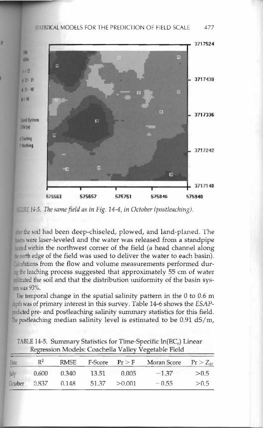
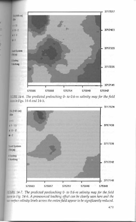