Chapter 15

1D Regression

... estimates of the linear regression coefficients are relevant to the linearparameters of a broader class of models than might have been suspected.

Brillinger (1977, p. 509)After computing β, one may go on to prepare a scatter plot of the points

(βxj, yj), j = 1, ..., n and look for a functional form for g(·).Brillinger (1983, p. 98)

Regression is the study of the conditional distribution Y |x of the responseY given the (p − 1) × 1 vector of nontrivial predictors x. The scalar Y is arandom variable and x is a random vector. A special case of regression ismultiple linear regression. In Chapter 2 the multiple linear regression modelwas Yi = wi,1η1 +wi,2η2 + · · ·+wi,pηp + ei = wT

i η+ ei for i = 1, . . . , n. In thischapter, the subscript i is often suppressed and the multiple linear regressionmodel is written as Y = α + x1β1 + · · · + xp−1βp−1 + e = α + βTx + e. Theprimary difference is the separation of the constant term α and the nontrivialpredictors x. In Chapter 2, wi,1 ≡ 1 for i = 1, ..., n. Taking Y = Yi, α = η1,βj = ηj+1, and xj = wi,j+1 and e = ei for j = 1, ..., p − 1 shows that thetwo models are equivalent. The change in notation was made because thedistribution of the nontrivial predictors is very important for the theory ofthe more general regression models.

Definition 15.1: Cook and Weisberg (1999a, p. 414). In a 1Dregression model, the response Y is conditionally independent of x given asingle linear combination βT x of the predictors, written

Y x|βT x or Y x|(α + βTx). (15.1)

433

The 1D regression model is also said to have 1–dimensional structure or1D structure. An important 1D regression model, introduced by Li and Duan(1989), has the form

Y = g(α + βTx, e) (15.2)

where g is a bivariate (inverse link) function and e is a zero mean error thatis independent of x. The constant term α may be absorbed by g if desired.

Special cases of the 1D regression model (15.1) include many importantgeneralized linear models (GLMs) and the additive error single index model

Y = m(α + βTx) + e. (15.3)

Typically m is the conditional mean or median function. For example if allof the expectations exist, then

E[Y |x] = E[m(α + βTx)|x] + E[e|x] = m(α + βTx).

The multiple linear regression model is an important special case where m isthe identity function: m(α + βTx) = α + βT x. Another important specialcase of 1D regression is the response transformation model where

g(α + βTx, e) = t−1(α + βTx + e) (15.4)

and t−1 is a one to one (typically monotone) function. Hence

t(Y ) = α + βT x + e.

Chapter 16 shows that many survival models are 1D regression models, in-cluding the Cox (1972) proportional hazards model. Li and Duan (1989, p.1014) note that the class of 1D regression models also includes binary re-gression models, censored regression models, and certain projection pursuitmodels.

Definition 15.2. Regression is the study of the conditional distributionof Y |x. Focus is often on the mean function E(Y |x) and/or the variancefunction VAR(Y |x). There is a distribution for each value of x = xo suchthat Y |x = xo is defined. For a 1D regression,

E(Y |x = xo) = E(Y |βT x = βTxo) ≡ M(βTxo)

andVAR(Y |x = xo) = VAR(Y |βT x = βTxo) ≡ V (βTxo)

434

where M is the kernel mean function and V is the kernel variance function.

Notice that the mean and variance functions depend on the same linearcombination if the 1D regression model is valid. This dependence is typicalof GLMs where M and V are known kernel mean and variance functionsthat depend on the family of GLMs. See Cook and Weisberg (1999a, section23.1). A heteroscedastic regression model

Y = M(βT1 x) +

√V (βT

2 x) e (15.5)

is a 1D regression model if β2 = cβ1 for some scalar c.

In multiple linear regression, the difference between the response Yi and

the estimated conditional mean function α + βTxi is the residual. For more

general regression models this difference may not be the residual, and the

“discrepancy” Yi−M(βTxi) may not be estimating the error ei. To guarantee

that the residuals are estimating the errors, the following definition is usedwhen possible.

Definition 15.3: Cox and Snell (1968). Let the errors ei be iid withpdf f and assume that the regression model Yi = g(xi, η, ei) has a uniquesolution for ei :

ei = h(xi, η, Yi).

Then the ith residualei = h(xi, η, Yi)

where η is a consistent estimator of η.

Example 15.1. Let η = (α, βT )T . If Y = m(α + βT x) + e where m is

known, then e = Y − m(α + βTx). Hence ei = Yi − m(α + βTxi) which is

the usual definition of the ith residual for such models.

Dimension reduction can greatly simplify our understanding of the con-ditional distribution Y |x. If a 1D regression model is appropriate, then the(p − 1)–dimensional vector x can be replaced by the 1–dimensional scalarβT x with “no loss of information about the conditional distribution.” Cookand Weisberg (1999a, p. 411) define a sufficient summary plot (SSP) to be aplot that contains all the sample regression information about the conditionaldistribution Y |x of the response given the predictors.

435

Definition 15.4: If the 1D regression model holds, then Y x|(a+cβTx)for any constants a and c �= 0. The quantity a + cβTx is called a sufficientpredictor (SP), and a sufficient summary plot is a plot of any SP versus Y .

An estimated sufficient predictor (ESP) is α + βTx where β is an estimator

of cβ for some nonzero constant c. A response plot or estimated sufficientsummary plot (ESSP) is a plot of any ESP versus Y .

If there is only one predictor x, then the plot of x versus Y is both asufficient summary plot and a response plot, but generally only a responseplot can be made. Since a can be any constant, a = 0 is often used. Thefollowing section shows how to use the OLS regression of Y on x to obtainan ESP.

15.1 Estimating the Sufficient Predictor

Some notation is needed before giving theoretical results. Let x, a, t, and βbe (p − 1) × 1 vectors where only x is random.

Definition 15.5: Cook and Weisberg (1999a, p. 431). The predic-tors x satisfy the condition of linearly related predictors with 1D structureif

E[x|βT x] = a + tβT x. (15.6)

If the predictors x satisfy this condition, then for any given predictor xj,

E[xj|βTx] = aj + tjβTx.

Notice that β is a fixed (p− 1)× 1 vector. If x is elliptically contoured (EC)with 1st moments, then the assumption of linearly related predictors holdssince

E[x|bTx] = ab + tbbTx

for any nonzero (p − 1) × 1 vector b (see Lemma 14.4). The condition oflinearly related predictors is impossible to check since β is unknown, but thecondition is far weaker than the assumption that x is EC. The stronger ECcondition is often used since there are checks for whether this condition isreasonable, eg use the DD plot. The following proposition gives an equivalent

436

definition of linearly related predictors. Both definitions are frequently usedin the dimension reduction literature.

Proposition 15.1. The predictors x are linearly related iff

E[bT x|βTx] = ab + tbβTx (15.7)

for any (p − 1) × 1 constant vector b where ab and tb are constants thatdepend on b.

Proof. Suppose that the assumption of linearly related predictors holds.Then

E[bT x|βT x] = bT E[x|βTx] = bT a + bT tβT x.

Thus the result holds with ab = bT a and tb = bT t.Now assume that Equation (15.7) holds. Take bi = (0, ..., 0, 1, 0, ..., 0)T ,

the vector of zeroes except for a one in the ith position. Then by Definition15.5, E[x|βT x] = E[Ip−1x|βTx] =

E[

bT1 x...

bTp−1x

| βT x] =

a1 + t1βT x

...ap−1 + tp−1β

Tx

≡ a + tβTx.

QED

Following Cook (1998a, p. 143-144), assume that there is an objectivefunction

Ln(a, b) =1

n

n∑i=1

L(a + bT xi, Yi) (15.8)

where L(u, v) is a bivariate function that is a convex function of the firstargument u. Assume that the estimate (a, b) of (a, b) satisfies

(a, b) = arg mina,b

Ln(a, b). (15.9)

For example, the ordinary least squares (OLS) estimator uses

L(a + bT x, Y ) = (Y − a − bTx)2.

Maximum likelihood type estimators such as those used to compute GLMsand Huber’s M–estimator also work, as does the Wilcoxon rank estima-tor. Assume that the population analog (α∗, β∗) is the unique minimizer of

437

E[L(a+bTx, Y )] where the expectation exists and is with respect to the jointdistribution of (Y, xT )T . For example, (α∗, β∗) is unique if L(u, v) is strictlyconvex in its first argument. The following result is a useful extension ofBrillinger (1977, 1983).

Theorem 15.2 (Li and Duan 1989, p. 1016): Assume that the x arelinearly related predictors, that (Yi, x

Ti )T are iid observations from some joint

distribution with Cov(xi) nonsingular. Assume L(u, v) is convex in its firstargument and that β∗ is unique. Assume that Y x|βTx. Then β∗ = cβfor some scalar c.

Proof. See Li and Duan (1989) or Cook (1998a, p. 144).

Remark 15.1. This theorem basically means that if the 1D regressionmodel is appropriate and if the condition of linearly related predictors holds,then the (eg OLS) estimator b ≡ β

∗ ≈ cβ. Li and Duan (1989, p. 1031)show that under additional conditions, (a, b) is asymptotically normal. Inparticular, the OLS estimator frequently has a

√n convergence rate. If the

OLS estimator (α, β) satisfies β ≈ cβ when model (15.1) holds, then theresponse plot of

α + βTx versus Y

can be used to visualize the conditional distribution Y |(α + βT x) providedthat c �= 0.

Remark 15.2. If b is a consistent estimator of β∗, then certainly

β∗ = cxβ + ug

where ug = β∗ − cxβ is the bias vector. Moreover, the bias vector ug = 0if x is elliptically contoured under the assumptions of Theorem 15.2. Thisresult suggests that the bias vector might be negligible if the distribution ofthe predictors is close to being EC. Often if no strong nonlinearities arepresent among the predictors, the bias vector is small enough so that

bTx is a useful ESP.

Remark 15.3. Suppose that the 1D regression model is appropriate andY x|βTx. Then Y x|cβT x for any nonzero scalar c. If Y = g(βT x, e)and both g and β are unknown, then g(βT x, e) = ha,c(a + cβTx, e) where

ha,c(w, e) = g(w − a

c, e)

438

for c �= 0. In other words, if g is unknown, we can estimate cβ but we cannot determine c or β; ie, we can only estimate β up to a constant.

A very useful result is that if Y = m(x) for some function m, then mcan be visualized with both a plot of x versus Y and a plot of cx versusY if c �= 0. In fact, there are only three possibilities, if c > 0 then the twoplots are nearly identical: except the labels of the horizontal axis change.(The two plots are usually not exactly identical since plotting controls to“fill space” depend on several factors and will change slightly.) If c < 0,then the plot appears to be flipped about the vertical axis. If c = 0, thenm(0) is a constant, and the plot is basically a dot plot. Similar results holdif Yi = g(α + βTxi, ei) if the errors ei are small. OLS often provides a usefulestimator of cβ where c �= 0, but OLS can result in c = 0 if g is symmetricabout the median of α + βTx.

Definition 15.6. If the 1D regression model (15.1) holds, and a specificestimator such as OLS is used, then the ESP will be called the OLS ESPand the response plot will be called the OLS response plot.

Example 15.2. Suppose that xi ∼ N3(0, I3) and that

Y = m(βT x) + e = (x1 + 2x2 + 3x3)3 + e.

Then a 1D regression model holds with β = (1, 2, 3)T . Figure 1.11 shows thesufficient summary plot of βTx versus Y , and Figure 1.12 shows the sufficientsummary plot of −βTx versus Y . Notice that the functional form m appearsto be cubic in both plots and that both plots can be smoothed by eye or witha scatterplot smoother such as lowess. The two figures were generated withthe following R/Splus commands.

X <- matrix(rnorm(300),nrow=100,ncol=3)

SP <- X%*%1:3

Y <- (SP)^3 + rnorm(100)

plot(SP,Y)

plot(-SP,Y)

We particularly want to use the OLS estimator (α, β) to produce anestimated sufficient summary plot. This estimator is obtained from the usualmultiple linear regression of Yi on xi, but we are not assuming that themultiple linear regression model holds; however, we are hoping that the 1D

439

regression model Y x|βT x is a useful approximation to the data and thatβ ≈ cβ for some nonzero constant c. In addition to Theorem 15.2, niceresults exist if the single index model is appropriate. Recall that

Cov(x, Y ) = E[(x− E(x))((Y − E(Y ))T ].

Definition 15.7. Suppose that (Yi, xTi )T are iid observations and that

the positive definite (p − 1) × (p − 1) matrix Cov(x) = ΣX and the (p −1)× 1 vector Cov(x, Y ) = ΣX,Y . Let the OLS estimator (α, β) be computed

from the multiple linear regression of Y on x plus a constant. Then (α, β)estimates the population quantity (αOLS, βOLS) where

αOLS = E(Y ) − βTOLSE(x) and βOLS = Σ−1

X ΣX,Y. (15.10)

The following notation will be useful for studying the OLS estimator.Let the sufficient predictor z = βTx and let w = x − E(x). Let r =w − (ΣXβ)βTw.

Theorem 15.3. In addition to the conditions of Definition 15.7, alsoassume that Yi = m(βTxi) + ei where the zero mean constant variance iiderrors ei are independent of the predictors xi. Then

βOLS = Σ−1X ΣX,Y = cm,Xβ + um,X (15.11)

where the scalarcm,X = E[βT (x − E(x)) m(βTx)] (15.12)

and the bias vectorum,X = Σ−1

X E[m(βTx)r]. (15.13)

Moreover, um,X = 0 if x is from an EC distribution with nonsingular ΣX,and cm,X �= 0 unless Cov(x, Y ) = 0. If the multiple linear regression modelholds, then cm,X = 1, and um,X = 0.

The proof of the above result is outlined in Problem 15.2 using an ar-gument due to Aldrin, Bφlviken, and Schweder (1993). If the 1D regressionmodel is appropriate, then typically Cov(x, Y ) �= 0 unless βT x follows asymmetric distribution and m is symmetric about the median of βTx.

Definition 15.8. Let (α, β) denote the OLS estimate obtained from theOLS multiple linear regression of Y on x. The OLS view is a response plot

of a + βTx versus Y . Typically a = 0 or a = α.

440

Remark 15.4. All of this awkward notation and theory leads to a ratherremarkable result, perhaps first noted by Brillinger (1977, 1983) and calledthe 1D Estimation Result by Cook and Weisberg (1999a, p. 432). The resultis that if the 1D regression model is appropriate, then the OLS view willfrequently be a useful estimated sufficient summary plot (ESSP). Hence the

OLS predictor βTx is a useful estimated sufficient predictor (ESP).

Although the OLS view is frequently a good ESSP if no strong nonlinear-ities are present in the predictors and if cm,X �= 0 (eg the sufficient summaryplot of βTx versus Y is not approximately symmetric), even better estimatedsufficient summary plots can be obtained by using ellipsoidal trimming. Thistopic is discussed in the following section and follows Olive (2002) closely.

15.2 Visualizing 1D Regression

If there are two predictors, even with a distribution that is not EC, Cookand Weisberg (1999a, ch. 8) demonstrate that a 1D regression can be visual-ized using a three–dimensional plot with Y on the vertical axes and the twopredictors on the horizontal and out of page axes. Rotate the plot about thevertical axes. Each combination of the predictors gives a two dimensional“view.” Search for the view with a smooth mean function that has the small-est possible variance function and use this view as the estimated sufficientsummary plot.

For higher dimensions, Cook and Nachtsheim (1994) and Cook (1998a, p.152) demonstrate that the bias um,X can often be made small by ellipsoidaltrimming. To perform ellipsoidal trimming, an estimator (T, C) is computedwhere T is a (p − 1) × 1 multivariate location estimator and C is a (p −1) × (p − 1) symmetric positive definite dispersion estimator. Then the ithsquared Mahalanobis distance is the random variable

D2i = (xi − T )TC−1(xi − T ) (15.14)

for each vector of observed predictors xi. If the ordered distances D(j) areunique, then j of the xi are in the hyperellipsoid

{x : (x − T )TC−1(x − T ) ≤ D2(j)}. (15.15)

The ith case (Yi, xTi )T is trimmed if Di > D(j). Thus if j ≈ 0.9n, then about

10% of the cases are trimmed.

441

We suggest that the estimator (T, C) should be the classical sample meanand covariance matrix (x, S) or a robust estimator such as covfch. Whenj ≈ n/2, the covfch estimator attempts to make the volume of the hyperel-lipsoid given by Equation (15.15) small.

Ellipsoidal trimming seems to work for at least three reasons. The trim-ming divides the data into two groups: the trimmed cases and the remainingcases (xM , YM ) where M% is the amount of trimming, eg M = 10 for 10%trimming. If the distribution of the predictors x is EC then the distributionof xM still retains enough symmetry so that the bias vector is approximatelyzero. If the distribution of x is not EC, then the distribution of xM willoften have enough symmetry so that the bias vector is small. In particular,trimming often removes strong nonlinearities from the predictors and theweighted predictor distribution is more nearly elliptically symmetric thanthe predictor distribution of the entire data set (recall Winsor’s principle:“all data are roughly Gaussian in the middle”). Secondly, under heavy trim-ming, the mean function of the remaining cases may be more linear than themean function of the entire data set. Thirdly, if |c| is very large, then the biasvector may be small relative to cβ. Trimming sometimes inflates |c|. FromTheorem 15.3, any of these three reasons should produce a better estimatedsufficient predictor.

Example 15.3. Cook and Weisberg (1999a, p. 351, 433, 447) gave adata set on 82 mussels sampled off the coast of New Zealand. The variablesare the muscle mass M in grams, the length L and height H of the shellin mm, the shell width W and the shell mass S. The robust and classicalMahalanobis distances were calculated, and Figure 15.1 shows a scatterplotmatrix of the mussel data, the RDi’s, and the MDi’s. Notice that manyof the subplots are nonlinear. The cases marked by open circles were givenweight zero by the cov.mcd algorithm, and the linearity of the retained caseshas increased. Note that only one trimming proportion is shown and thata heavier trimming proportion would increase the linearity of the cases thatwere not trimmed.

The two ideas of using ellipsoidal trimming to reduce the bias and choos-ing a view with a smooth mean function and smallest variance function canbe combined into a graphical method for finding the estimated sufficient sum-mary plot and the estimated sufficient predictor. Trim the M% of the caseswith the largest Mahalanobis distances, and then compute the OLS estima-

442

Figure 15.1: Scatterplot for Mussel Data, o Corresponds to Trimmed Cases

443

tor (αM , βM ) from the cases that remain. Use M = 0, 10, 20, 30, 40, 50, 60,

70, 80, and 90 to generate ten plots of βT

Mx versus Y using all n cases. Inanalogy with the Cook and Weisberg procedure for visualizing 1D structurewith two predictors, the plots will be called “trimmed views.” Notice thatM = 0 corresponds to the OLS view.

Definition 15.9. The best trimmed view is the trimmed view with asmooth mean function and the smallest variance function and is the estimatedsufficient summary plot. If M∗ = E is the percentage of cases trimmed that

corresponds to the best trimmed view, then βT

Ex or αE+βT

Ex is the estimatedsufficient predictor.

The following examples illustrate the R/Splus regpack function trviews

that is used to produce the ESSP. If R is used instead of Splus, the command

library(MASS)

needs to be entered to access the function cov.mcd called by trviews. Therobust estimators cov.fch and cov.mbacan also be used. The functiontrviews is used in Problem 15.6. The estimator can be used to simultane-ously detect whether the data is following a multiple linear regression model

or some other single index model. Plot αE + βT

Ex versus Y and add the iden-tity line. If the plotted points follow the identity line then the MLR model isreasonable, but if the plotted points follow a nonlinear mean function, thena nonlinear single index model may be reasonable.

Example 15.2 continued. The command

trviews(X, Y)

produced the following output.

Intercept X1 X2 X3

0.6701255 3.133926 4.031048 7.593501

Intercept X1 X2 X3

1.101398 8.873677 12.99655 18.29054

Intercept X1 X2 X3

0.9702788 10.71646 15.40126 23.35055

Intercept X1 X2 X3

0.5937255 13.44889 23.47785 32.74164

444

Intercept X1 X2 X3

1.086138 12.60514 25.06613 37.25504

Intercept X1 X2 X3

4.621724 19.54774 34.87627 48.79709

Intercept X1 X2 X3

3.165427 22.85721 36.09381 53.15153

Intercept X1 X2 X3

5.829141 31.63738 56.56191 82.94031

Intercept X1 X2 X3

4.241797 36.24316 70.94507 105.3816

Intercept X1 X2 X3

6.485165 41.67623 87.39663 120.8251

The function generates 10 trimmed views. The first plot trims 90% of thecases while the last plot does not trim any of the cases and is the OLS view.To advance a plot, press the right button on the mouse (in R, highlightstop rather than continue). After all of the trimmed views have beengenerated, the output is presented. For example, the 5th line of numbers in

the output corresponds to α50 = 1.086138 and βT

50 where 50% trimming wasused. The second line of numbers corresponds to 80% trimming while the

last line corresponds to 0% trimming and gives the OLS estimate (α0, βT

0 ) =(a, b). The trimmed views with 50% and 90% trimming were very good.We decided that the view with 50% trimming was the best. Hence βE =(12.60514, 25.06613, 37.25504)T ≈ 12.5β. The best view is shown in Figure15.2 and is nearly identical to the sufficient summary plot shown in Figure1.11. Notice that the OLS estimate = (41.68, 87.40, 120.83)T ≈ 42β. TheOLS view is shown in Figure 1.13, and is again very similar to the sufficientsummary plot, but it is not quite as smooth as the best trimmed view.

The plot of the estimated sufficient predictor versus the sufficient predic-tor is also informative. Of course this plot can usually only be generated forsimulated data since β is generally unknown. If the plotted points are highlycorrelated (with |corr(ESP,SP)| > 0.95) and follow a line through the origin,then the estimated sufficient summary plot is nearly as good as the sufficientsummary plot. The simulated data used β = (1, 2, 3)T , and the commands

SP <- X %*% 1:3

ESP <- X %*% c(12.60514, 25.06613, 37.25504)

plot(ESP,SP)

445

ESP

Y

-100 -50 0 50 100

-500

050

0

ESSP for Gaussian Predictors

Figure 15.2: Best View for Estimating m(u) = u3

ESP

SP

-100 -50 0 50 100

-10

-50

510

CORR(ESP,SP) is Approximately One

Figure 15.3: The angle between the SP and the ESP is nearly zero.

446

generated the plot shown in Figure 15.3.

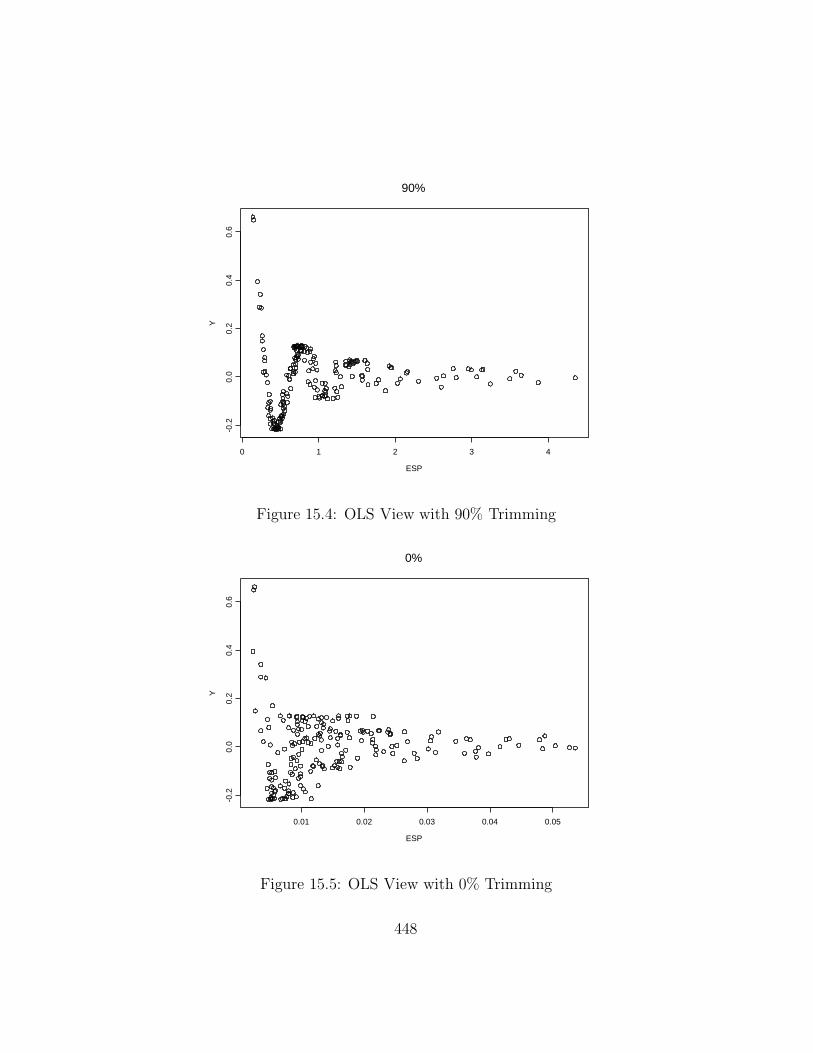
Example 15.4. An artificial data set with 200 trivariate vectors xi

was generated. The marginal distributions of xi,j are iid lognormal forj = 1, 2, and 3. Since the response Yi = sin(βT xi)/β

Txi where β =(1, 2, 3)T , the random vector xi is not elliptically contoured and the func-

tion m is strongly nonlinear. Figure 15.5 shows the OLS view where βT

0 =(0.0032, 0.0011, 0.0047)T and Figure 15.4 shows the best trimmed view where

βT

90 = (0.086, 0.182, 0.338)T ≈ 0.1β, roughly. Notice that it is difficult to vi-sualize the mean function with the OLS view, and notice that the correlationbetween Y and the ESP is very low. By focusing on a part of the data wherethe correlation is high, it may be possible to improve the estimated sufficientsummary plot. For example, in Figure 15.4, temporarily omit cases thathave ESP less than 0.3 and greater than 0.75. From the untrimmed cases,obtained the ten trimmed estimates β90, ..., β0. Then using all of the data,obtain the ten views. The best view could be used as the ESSP.

Application 15.1. Suppose that a 1D regression analysis is desired ona data set, use the trimmed views as an exploratory data analysis techniqueto visualize the conditional distribution Y |βT x. The best trimmed view isan estimated sufficient summary plot. If the single index model (15.3) holds,the function m can be estimated from this plot using parametric modelsor scatterplot smoothers such as lowess. Notice that Y can be predictedvisually using up and over lines.

Application 15.2. The best trimmed view can also be used as a diag-nostic for linearity and monotonicity.

For example in Figure 15.2, if ESP = 0, then Y = 0 and if ESP = 100,then Y = 500. Figure 15.2 suggests that the mean function is monotone butnot linear, and Figure 15.4 suggests that the mean function is neither linearnor monotone.

Application 15.3. Assume that a known 1D regression model is as-sumed for the data. Then the best trimmed view can be used as a diagnosticfor whether the assumed model is appropriate.

The trimmed views are sometimes useful even when the assumption oflinearly related predictors fails. OLS frequently performs well if there are nostrong nonlinearities present in the predictors.

447

ESP

Y

0 1 2 3 4

-0.2

0.0

0.2

0.4

0.6

90%

Figure 15.4: OLS View with 90% Trimming

ESP

Y

0.01 0.02 0.03 0.04 0.05

-0.2

0.0

0.2

0.4

0.6

0%

Figure 15.5: OLS View with 0% Trimming

448

15.3 Predictor Transformations

As a general rule, inferring about the distribution of Y |X from a lowerdimensional plot should be avoided when there are strong nonlinearities

among the predictors.Cook and Weisberg (1999b, p. 34)

Even if the multiple linear regression model is valid, a model based on asubset of the predictor variables depends on the predictor distribution. If thepredictors are linearly related (eg EC), then the submodel mean and vari-ance functions are generally well behaved, but otherwise the submodel meanfunction could be nonlinear and the submodel variance function could benonconstant. For 1D regression models, the presence of strong nonlinearitiesamong the predictors can invalidate inferences. A necessary condition forx to have an EC distribution (or for no strong nonlinearities to be presentamong the predictors) is for each marginal plot of the scatterplot matrix ofthe predictors to have a linear or ellipsoidal shape if n is large.

One of the most useful techniques in regression is to remove gross nonlin-earities in the predictors by using predictor transformations. Power trans-formations are particularly effective. A multivariate version of the Box–Coxtransformation due to Velilla (1993) can cause the distribution of the trans-formed predictors to be closer to multivariate normal, and the Cook andNachtsheim (1994) procedure can cause the distribution to be closer to ellip-tical symmetry. Marginal Box-Cox transformations also seem to be effective.Power transformations can also be selected with slider bars in Arc.

There are several rules for selecting marginal transformations visually.(Also see discussion in Section 3.1.) First, use theory if available. Supposethat variable X2 is on the vertical axis and X1 is on the horizontal axis andthat the plot of X1 versus X2 is nonlinear. The unit rule says that if X1 andX2 have the same units, then try the same transformation for both X1 andX2.

Power transformations are also useful. Assume that all values of X1 andX2 are positive. Let λ be the power of the transformation. Then the followingfour rules are often used.

The log rule states that positive predictors that have the ratio betweentheir largest and smallest values greater than ten should be transformed tologs. See Cook and Weisberg (1999a, p. 87).

Secondly, if it is known that X2 ≈ Xλ1 and the ranges of X1 and X2 are

449

such that this relationship is one to one, then

Xλ1 ≈ X2 and X

1/λ2 ≈ X1.

Hence either the transformation Xλ1 or X

1/λ2 will linearize the plot. This

relationship frequently occurs if there is a volume present. For example letX2 be the volume of a sphere and let X1 be the circumference of a sphere.The plot of log(X1) versus log(X2) will also be linear.

Thirdly, the bulging rule states that changes to the power of X2 and thepower of X1 can be determined by the direction that the bulging side of thecurve points. If the curve is hollow up (the bulge points down), decrease thepower of X2. If the curve is hollow down (the bulge points up), increase thepower of X2 If the curve bulges towards large values of X1 increase the powerof X1. If the curve bulges towards small values of X1 decrease the power ofX1. See Tukey (1977, p. 173–176).

Finally, Cook and Weisberg (1999a, p. 86) give the following rule.To spread small values of a variable, make λ smaller.To spread large values of a variable, make λ larger.

For example, in Figure 15.10c, small values of Y and large values of FESPneed spreading, and using log(Y ) would make the plot more linear.

15.4 Variable Selection

A standard problem in 1D regression is variable selection, also called subset ormodel selection. Assume that model (15.1) holds, that a constant is alwaysincluded, and that x = (x1, ..., xp−1)

T are the p − 1 nontrivial predictors,which we assume to be of full rank. Then variable selection is a search fora subset of predictor variables that can be deleted without important loss ofinformation. This section follows Olive and Hawkins (2005) closely.

Variable selection for the 1D regression model is very similar to variableselection for the multiple linear regression model (see Section 3.4). To clarifyideas, assume that there exists a subset S of predictor variables such thatif xS is in the 1D model, then none of the other predictors are needed inthe model. Write E for these (‘extraneous’) variables not in S, partitioningx = (xT

S , xTE)T . Then

SP = α + βT x = α + βTSxS + βT

ExE = α + βTSxS. (15.16)

450

The extraneous terms that can be eliminated given that the subset S is inthe model have zero coefficients.

Now suppose that I is a candidate subset of predictors, that S ⊆ I andthat O is the set of predictors not in I . Then

SP = α + βTx = α + βTSxS = α + βT

SxS + βT(I/S)xI/S + 0TxO = α + βT

I xI ,

(if I includes predictors from E, these will have zero coefficient). For anysubset I that contains the subset S of relevant predictors, the correlation

corr(α + βTxi, α + βTI xI,i) = 1. (15.17)

This observation, which is true regardless of the explanatory power ofthe model, suggests that variable selection for 1D regression models is simplein principle. For each value of j = 1, 2, ..., p − 1 nontrivial predictors, keeptrack of subsets I that provide the largest values of corr(ESP,ESP(I)). Anysuch subset for which the correlation is high is worth closer investigationand consideration. To make this advice more specific, use the rule of thumbthat a candidate subset of predictors I is worth considering if the samplecorrelation of ESP and ESP(I) satisfies

corr(α + βTxi, αI + β

T

I xI,i) = corr(βTxi, β

T

I xI,i) ≥ 0.95. (15.18)

The difficulty with this approach is that fitting all of the possible sub-models involves substantial computation. An exception to this difficulty ismultiple linear regression where there are efficient “leaps and bounds” algo-rithms for searching all subsets when OLS is used (see Furnival and Wilson1974). Since OLS often gives a useful ESP, the following all subsets procedurecan be used for 1D models when p < 20.

• Fit a full model using the methods appropriate to that 1D problem to

find the ESP α + βTx.

• Find the OLS ESP αOLS + βT

OLSx.

• If the 1D ESP and the OLS ESP have “a strong linear relationship”(for example |corr(ESP, OLS ESP)| ≥ 0.95), then infer that the 1Dproblem is one in which OLS may serve as an adequate surrogate forthe correct 1D model fitting procedure.

451

• Use computationally fast OLS variable selection procedures such asforward selection, backward elimination and the leaps and bounds al-gorithm along with the Mallows (1973) Cp criterion to identify pre-dictor subsets I containing k variables (including the constant) withCp(I) ≤ min(2k, p).

• Perform a final check on the subsets that satisfy the Cp screen by usingthem to fit the 1D model.

For a 1D model, the response, ESP and vertical discrepancies V =Y −ESP are important. When the multiple linear regression (MLR) modelholds, the fitted values are the ESP: Y = ESP , and the vertical discrepanciesare the residuals.

Definition 15.10. a) The plot of αI + βT

I xI,i versus α + βTxi is called

an EE plot (often called an FF plot for MLR).

b) The plot of discrepancies Yi − αI − βT

I xI,i versus Yi − α − βTxi is called

a VV plot (often called an RR plot for MLR).

c) The plots of αI + βT

I xI,i versus Yi and of α + βTxi versus Yi are called

estimated sufficient summary plots or response plots.

Many numerical methods such as forward selection, backward elimination,stepwise and all subset methods using the Cp criterion (Jones 1946, Mallows1973), have been suggested for variable selection. The four plots in Definition15.10 contain valuable information to supplement the raw numerical resultsof these selection methods. Particular uses include:

• The key to understanding which plots are the most useful is the obser-vation that a wz plot is used to visualize the conditional distributionof z given w. Since a 1D regression is the study of the conditionaldistribution of Y given α + βTx, the response plot is used to visual-ize this conditional distribution and should always be made. A majorproblem with variable selection is that deleting important predictorscan change the functional form m of the model. In particular, if a mul-tiple linear regression model is appropriate for the full model, linearitymay be destroyed if important predictors are deleted. When the singleindex model (15.3) holds, m can be visualized with a response plot.Adding visual aids such as the estimated parametric mean function

452

m(α + βTx) can be useful. If an estimated nonparametric mean func-

tion m(α + βTx) such as lowess follows the parametric curve closely,

then often numerical goodness of fit tests will suggest that the model isgood. See Chambers, Cleveland, Kleiner, and Tukey (1983, p. 280) andCook and Weisberg (1999a, p. 425, 432). For variable selection, theresponse plots from the full model and submodel should be very similarif the submodel is good.

• Sometimes outliers will influence numerical methods for variable selec-tion. Outliers tend to stand out in at least one of the plots. An EE plotis useful for variable selection because the correlation of ESP(I) andESP is important. The EE plot can be used to quickly check that thecorrelation is high, that the plotted points fall about some line, thatthe line is the identity line, and that the correlation is high because therelationship is linear, rather than because of outliers.

• Numerical methods may include too many predictors. Investigators canexamine the p–values for individual predictors, but the assumptionsneeded to obtain valid p–values are often violated; however, the OLS ttests for individual predictors are meaningful since deleting a predictorchanges the Cp value by t2 − 2 where t is the test statistic for thepredictor. See Section 15.5, Daniel and Wood (1980, p. 100-101) andthe following two remarks.

Remark 15.5. Variable selection with the Cp criterion is closely relatedto the partial F test that uses test statistic FI. Suppose that the full modelcontains p predictors including a constant and the submodel I includes k pre-dictors including a constant. If n ≥ 10p, then the submodel I is “interesting”if Cp(I) ≤ min(2k, p).

To see this claim notice that the following results are properties of OLSand hold even if the data does not follow a 1D model. If the candidate modelof xI has k terms (including the constant), then

FI =SSE(I)− SSE

(n − k) − (n − p)/

SSE

n − p=

n − p

p − k

[SSE(I)

SSE− 1

]where SSE is the “residual” sum of squares from the full model and SSE(I)is the “residual” sum of squares from the candidate submodel. Then

Cp(I) =SSE(I)

MSE+ 2k − n = (p − k)(FI − 1) + k (15.19)

453

where MSE is the “residual” mean square for the full model. Let ESP(I) =

αI + βT

I xI be the ESP for the submodel and let VI = Y − ESP (I) so that

VI,i = Yi − αI + βT

I xI,i. Let ESP and V denote the corresponding quantitiesfor the full model. Using Proposition 3.2 and Remark 3.2 with corr(r, rI)replaced by corr(V, VI), it can be shown that

corr(V, VI ) =

√SSE

SSE(I)=

√n − p

Cp(I) + n − 2k=

√n − p

(p − k)FI + n − p.

It can also be shown that Cp(I) ≤ 2k corresponds to corr(V, VI) ≥ dn where

dn =

√1 − p

n.

Notice that for a fixed value of k, the submodel Ik that minimizes Cp(I) alsomaximizes corr(V, VI ). If Cp(I) ≤ 2k and n ≥ 10p, then 0.948 ≤ corr(V, VI),and both corr(V, VI) → 1.0 and corr(OLS ESP, OLS ESP(I)) → 1.0 asn → ∞. Hence the plotted points in both the VV plot and the EE plot willcluster about the identity line (see Proposition 3.2).

Remark 15.6. Suppose that the OLS ESP and the standard ESP arehighly correlated: |corr(ESP, OLS ESP)| ≥ 0.95. Then often OLS variableselection can be used for the 1D data, and using the p–values from OLSoutput seems to be a useful benchmark. To see this, suppose that n > 5pand first consider the model Ii that deletes the predictor Xi. Then model Ii

has k = p − 1 predictors including the constant, and the test statistic is ti

wheret2i = FIi.

Using (15.19) and Cp(Ifull) = p, it can be shown that

Cp(Ii) = Cp(Ifull) + (t2i − 2).

Using the screen Cp(I) ≤ min(2k, p) suggests that the predictor Xi shouldnot be deleted if

|ti| >√

2 ≈ 1.414.

If |ti| <√

2 then the predictor can probably be deleted since Cp decreases.More generally, it can be shown that Cp(I) ≤ 2k iff

FI ≤ p

p − k.

454

Now k is the number of terms in the model including a constant while p− kis the number of terms set to 0. As k → 0, the partial F test will reject Ho:βO = 0 (ie, say that the full model should be used instead of the submodelI) unless FI is not much larger than 1. If p is very large and p − k is verysmall, then the change in SS F test will tend to suggest that there is a modelI that is about as good as the full model even though model I deletes p − kpredictors.

The Cp(I) ≤ k screen tends to overfit. We simulated multiple linearregression and single index model data sets with p = 8 and n = 50, 100, 1000and 10000. The true model S satisfied Cp(S) ≤ k for about 60% of thesimulated data sets, but S satisfied Cp(S) ≤ 2k for about 97% of the datasets.

In many settings, not all of which meet the Li–Duan sufficient conditions,the full model OLS ESP is a good estimator of the sufficient predictor. Ifthe fitted full 1D model Y x|(α + βT x) is a useful approximation to thedata and if βOLS is a good estimator of cβ where c �= 0, then a subset Iwill produce a response plot similar to the response plot of the full modelif corr(OLS ESP, OLS ESP(I)) ≥ 0.95. Hence the response plots based onthe full and submodel ESP can both be used to visualize the conditionaldistribution of Y .

Assuming that a 1D model holds, a common assumption made for variableselection is that the fitted full model ESP is a good estimator of the sufficientpredictor, and the usual numerical and graphical checks on this assumptionshould be made. To see that this assumption is weaker than the assumptionthat the OLS ESP is good, notice that if a 1D model holds but βOLS estimatescβ where c = 0, then the Cp(I) criterion could wrongly suggest that allsubsets I have Cp(I) ≤ 2k. Hence we also need to check that c �= 0.

There are several methods are for checking the OLS ESP, including: a) ifan ESP from an alternative fitting method is believed to be useful, check thatthe ESP and the OLS ESP have a strong linear relationship: for examplethat |corr(ESP, OLS ESP)| ≥ 0.95. b) Often examining the OLS responseplot shows that a 1D model is reasonable. For example, if the data are tightlyclustered about a smooth curve, then a single index model may be appro-priate. c) Verify that a 1D model is appropriate using graphical techniquesgiven by Cook and Weisberg (1999a, p. 434-441). d) Verify that x has anEC distribution with nonsingular covariance matrix and that the mean func-tion m(α + βT x) is not symmetric about the median of the distribution of

455

α + βTx. Then results from Li and Duan (1989) suggest that c �= 0.Condition a) is both the most useful (being a direct performance check)

and the easiest to check. A standard fitting method should be used whenavailable (eg, for parametric 1D models such as GLMs). Conditions c) andd) need x to have a continuous multivariate distribution while the predictorscan be factors for a) and b). Using trimmed views results in an ESP thatcan sometimes cause condition b) to hold when d) is violated.

To summarize, variable selection procedures, originally meant for MLR,can often be used for 1D data. If the fitted full 1D model Y x|(α + βTx)is a useful approximation to the data and if βOLS is a good estimator of cβwhere c �= 0, then a subset I is good if corr(OLS ESP, OLS ESP(I)) ≥ 0.95.If n is large enough, Remark 15.5 implies that this condition will hold ifCp(I) ≤ 2k or if FI ≤ 1. This result suggests that within the (large) subclassof 1D models where the OLS ESP is useful, the OLS partial F test is robust(asymptotically) to model misspecifications in that FI ≤ 1 correctly suggeststhat submodel I is good. The OLS t tests for individual predictors are alsomeaningful since if |t| <

√2 then the predictor can probably be deleted since

Cp decreases while if |t| ≥ 2 then the predictor is probably useful even whenthe other predictors are in the model. Section 15.5 provides related theory,and the following examples help illustrate the above discussion.

Example 15.5. This example illustrates that the plots are useful forgeneral 1D regression models such as the response transformation model.Cook and Weisberg (1999a, p. 351, 433, 447, 463) describe a data set on 82mussels. The response Y is the muscle mass in grams, and the four predictorsare the logarithms of the shell length, width, height and mass. The logarithmtransformation was used to remove strong nonlinearities that were evidentin a scatterplot matrix of the untransformed predictors. The Cp criterionsuggests using log(width) and log(shell mass) as predictors. The EE and VVplots are shown in Figure 15.6ab. The response plots based on the full andsubmodel are shown in Figure 15.6cd and are nearly identical, but not linear.

When log(muscle mass) is used as the response, the Cp criterion suggestsusing log(height) and log(shell mass) as predictors (the correlation betweenlog(height) and log(width) is very high). Figure 15.7a shows the RR plotand 2 outliers are evident. These outliers correspond to the two outliers inthe response plot shown in Figure 15.7b. After deleting the outliers, the Cp

criterion still suggested using log(height) and log(shell mass) as predictors.

456

SFIT

FF

IT

-10 0 10 20 30 40

-10

010

2030

40

a) EE Plot

SRES

FR

ES

-5 0 5 10 15

-10

-50

510

15

b) VV Plot

FFIT

Y

-10 0 10 20 30 40

010

2030

4050

c) Response Plot (Full)

SFIT

Y

-10 0 10 20 30 40

010

2030

4050

d) Response Plot (Sub)

Figure 15.6: Mussel Data with Muscle Mass as the Response

SRES

FR

ES

-1.0 -0.8 -0.6 -0.4 -0.2 0.0 0.2 0.4

-1.0

-0.6

-0.2

0.2

a) RR Plot with Two Outliers

SFIT

Y

1.0 1.5 2.0 2.5 3.0 3.5 4.0

01

23

4

b) Linear Response Plot

Figure 15.7: Mussel Data with log(Muscle Mass) as the Response

457

FFIT

Y

-4 -2 0 2

-4-2

02

4

a) Full Response Plot

FFIT

FR

ES

-4 -2 0 2

-2-1

01

2

b) Full Residual Plot

SFIT

Y

-4 -2 0 2

-4-2

02

4

c) Submodel Response Plot

SFIT

SR

ES

-4 -2 0 2

-2-1

01

2

d) Submodel Residual Plot

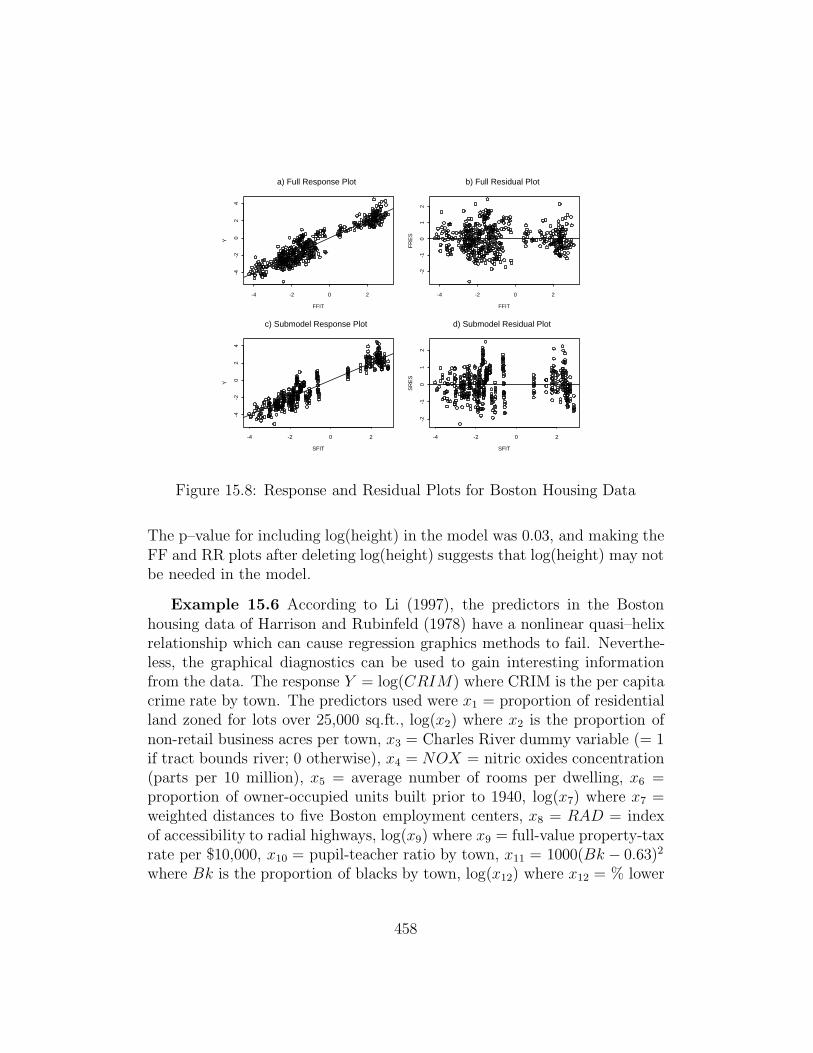
Figure 15.8: Response and Residual Plots for Boston Housing Data

The p–value for including log(height) in the model was 0.03, and making theFF and RR plots after deleting log(height) suggests that log(height) may notbe needed in the model.

Example 15.6 According to Li (1997), the predictors in the Bostonhousing data of Harrison and Rubinfeld (1978) have a nonlinear quasi–helixrelationship which can cause regression graphics methods to fail. Neverthe-less, the graphical diagnostics can be used to gain interesting informationfrom the data. The response Y = log(CRIM) where CRIM is the per capitacrime rate by town. The predictors used were x1 = proportion of residentialland zoned for lots over 25,000 sq.ft., log(x2) where x2 is the proportion ofnon-retail business acres per town, x3 = Charles River dummy variable (= 1if tract bounds river; 0 otherwise), x4 = NOX = nitric oxides concentration(parts per 10 million), x5 = average number of rooms per dwelling, x6 =proportion of owner-occupied units built prior to 1940, log(x7) where x7 =weighted distances to five Boston employment centers, x8 = RAD = indexof accessibility to radial highways, log(x9) where x9 = full-value property-taxrate per $10,000, x10 = pupil-teacher ratio by town, x11 = 1000(Bk − 0.63)2

where Bk is the proportion of blacks by town, log(x12) where x12 = % lower

458

SFIT2

Y

-3 -2 -1 0 1 2 3

-4-2

02

4

a) Response Plot with X4 and X8

NOX

RA

D

0.4 0.5 0.6 0.7 0.8

510

1520

b) Outliers in Predictors

Figure 15.9: Relationships between NOX, RAD and Y = log(CRIM)

status of the population, and log(x13) where x13 = median value of owner-occupied homes in $1000’s. The full model has 506 cases and 13 nontrivialpredictor variables.

Figure 15.8ab shows the response plot and residual plot for the full model.The residual plot suggests that there may be three or four groups of data,but a linear model does seem plausible. Backward elimination with Cp

suggested the “min Cp submodel” with the variables x1, log(x2), NOX, x6,log(x7), RAD, x10, x11 and log(x13). The full model had R2 = 0.878 and σ =0.7642. The Cp submodel had Cp(I) = 6.576, R2

I = 0.878, and σI = 0.762.Deleting log(x7) resulted in a model with Cp = 8.483 and the smallest coeffi-cient p–value was 0.0095. The FF and RR plots for this model (not shown)looked like the identity line. Examining further submodels showed that NOXand RAD were the most important predictors. In particular, the OLS coeffi-cients of x1, x6 and x11 were orders of magnitude smaller than those of NOXand RAD. The submodel including a constant, NOX, RAD and log(x2) hadR2 = 0.860, σ = 0.811 and Cp = 67.368. Figure 15.8cd shows the responseplot and residual plot for this submodel.

Although this submodel has nearly the same R2 as the full model, theresiduals show more variability than those of the full model. Nevertheless,

459

SUBV

FU

LLV

0 20 40 60

020

4060

a) VV Plot

SESP

FE

SP

0 5 10 15

05

1015

b) EE Plot

FESP

Y

0 5 10 15

020

4060

80

c) Full Model EY Plot

SESP

Y

0 5 10 15

020

4060

80

d) Submodel EY Plot

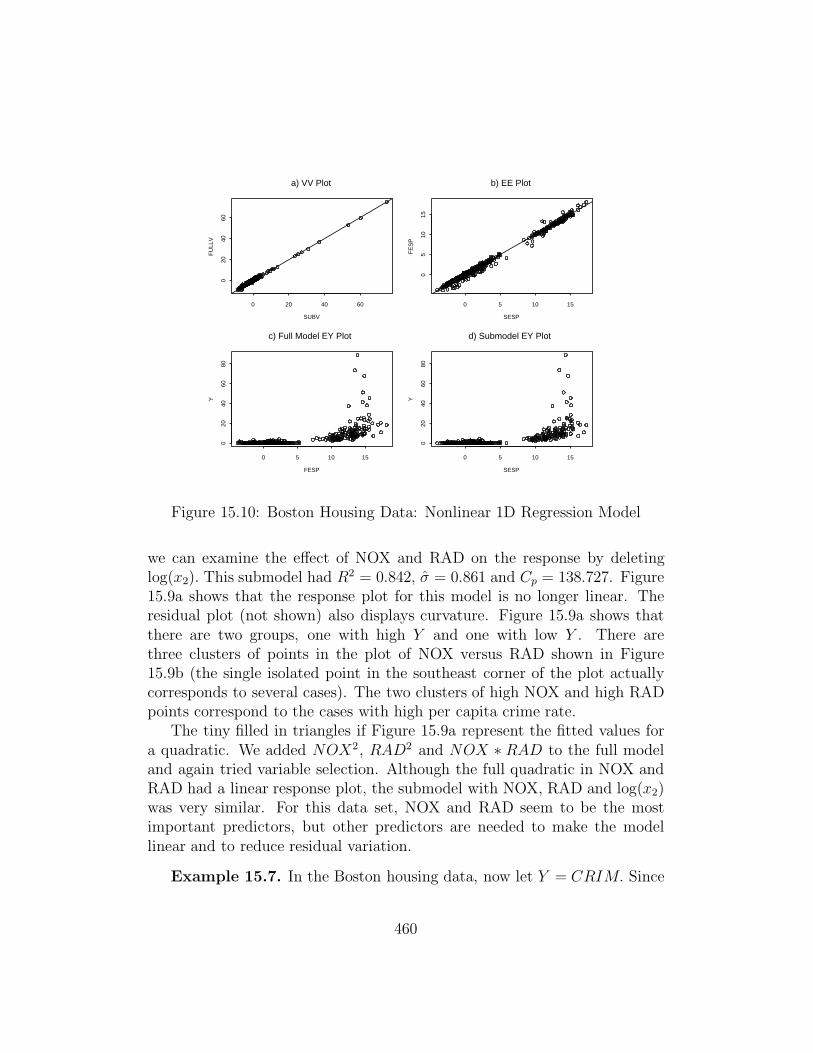
Figure 15.10: Boston Housing Data: Nonlinear 1D Regression Model

we can examine the effect of NOX and RAD on the response by deletinglog(x2). This submodel had R2 = 0.842, σ = 0.861 and Cp = 138.727. Figure15.9a shows that the response plot for this model is no longer linear. Theresidual plot (not shown) also displays curvature. Figure 15.9a shows thatthere are two groups, one with high Y and one with low Y . There arethree clusters of points in the plot of NOX versus RAD shown in Figure15.9b (the single isolated point in the southeast corner of the plot actuallycorresponds to several cases). The two clusters of high NOX and high RADpoints correspond to the cases with high per capita crime rate.

The tiny filled in triangles if Figure 15.9a represent the fitted values fora quadratic. We added NOX2, RAD2 and NOX ∗ RAD to the full modeland again tried variable selection. Although the full quadratic in NOX andRAD had a linear response plot, the submodel with NOX, RAD and log(x2)was very similar. For this data set, NOX and RAD seem to be the mostimportant predictors, but other predictors are needed to make the modellinear and to reduce residual variation.

Example 15.7. In the Boston housing data, now let Y = CRIM. Since

460

log(Y ) has a linear relationship with the predictors, Y should follow a nonlin-ear 1D regression model. Consider the full model with predictors log(x2), x3,x4, x5, log(x7), x8, log(x9) and log(x12). Regardless of whether Y or log(Y )is used as the response, the minimum Cp model from backward eliminationused a constant, log(x2), x4, log(x7), x8 and log(x12) as predictors. If Y is theresponse, then the model is nonlinear and Cp = 5.699. Remark 15.5 suggeststhat if Cp ≤ 2k, then the points in the VV plot should tightly cluster aboutthe identity line even if a multiple linear regression model fails to hold. Fig-ure 15.10 shows the VV and EE plots for the minimum Cp submodel. Theresponse (EY) plots for the full model and submodel are also shown. Notethat the clustering in the VV plot is indeed higher than the clustering in theEE plot. Note that the response plots are highly nonlinear but are nearlyidentical.

15.5 Inference

This section follows Chang and Olive (2010) closely. Inference can be per-formed for trimmed views if M is chosen without using the response, eg ifthe trimming is done with a DD plot, and the dimension reduction (DR)method such as OLS is performed on the data (YMi, xMi) that remains aftertrimming M% of the cases with ellipsoidal trimming based on the MBA orFCH estimator.

First we review some theoretical results for OLS as a DR method andgive the main theoretical result for OLS. Let

Cov(x) = E[(x− E(x))(x − E(x))T] = Σx

and Cov(x, Y ) = E[(x− E(x))(Y − E(Y ))] = ΣxY . Let the OLS estimatorbe (αOLS, βOLS). Then the population coefficients from an OLS regression ofY on x are

αOLS = E(Y ) − βTOLSE(x) and βOLS = Σ−1

x ΣxY. (15.20)

Let the data be (Yi, xi) for i = 1, ..., n. Let the p×1 vector η = (α, βT )T ,let X be the n × p OLS design matrix with ith row (1, xT

i ), and let Y =(Y1, ..., Yn)

T . Then the OLS estimator η = (XT X)−1XTY . The sample co-variance of x is

Σx =1

n − 1

n∑i=1

(xi − x)(xi − x)T where the sample mean x =1

n

n∑i=1

xi.

461

Similarly, define the sample covariance of x and Y to be

ΣxY =1

n

n∑i=1

(xi − x)(Yi − Y ) =1

n

n∑i=1

xiYi − x Y .

The first result shows that η is a consistent estimator of η.i) Suppose that (Yi, x

Ti )T are iid random vectors such that Σ−1

x and ΣxY

exist. ThenαOLS = Y − β

T

OLSxD→ αOLS

andβOLS =

n

n − 1Σ

−1

x ΣxYD→ βOLS as n → ∞.

The following OLS results need some notation. Many 1D regression mod-els have an error e with

σ2 = Var(e) = E(e2). (15.21)

Let e be the error residual for e. Let the population OLS residual

v = Y − αOLS − βTOLSx (15.22)

withτ 2 = E[(Y − αOLS − βT

OLSx)2] = E(v2), (15.23)

and let the OLS residual be

r = Y − αOLS − βT

OLSx. (15.24)

Typically the OLS residual r is not estimating the error e and τ 2 �= σ2, butthe following results show that the OLS residual is of great interest for 1Dregression models.

Assume that a 1D model holds, Y x|(α + βT x), which is equivalent toY x|βTx. Then under regularity conditions, results ii) – iv) below hold.

ii) Li and Duan (1989): βOLS = cβ for some constant c.iii) Li and Duan (1989) and Chen and Li (1998):

√n(βOLS − cβ)

D→ Np−1(0, COLS) (15.25)

where

COLS = Σ−1x E[(Y − αOLS − βT

OLSx)2(x −E(x))(x− E(x))T ]Σ−1x . (15.26)

462

iv) Chen and Li (1998): Let A be a known full rank constant k × (p− 1)matrix. If the null hypothesis Ho: Aβ = 0 is true, then

√n(AβOLS − cAβ) =

√nAβOLS

D→ Nk(0, ACOLSAT )

andACOLSAT = τ 2AΣ−1

x AT . (15.27)

Notice that COLS = τ 2Σ−1x if v = Y − αOLS − βT

OLSx x or if the MLRmodel holds. If the MLR model holds, τ 2 = σ2.

To create test statistics, the estimator

τ 2 = MSE =1

n − p

n∑i=1

r2i =

1

n − p

n∑i=1

(Yi − αOLS − βT

OLSxi)2

will be useful. The estimator COLS =

Σ−1

x

[1

n

n∑i=1

[(Yi − αOLS − βT

OLSxi)2(xi − x)(xi − x)T ]

]Σ

−1

x (15.28)

can also be useful. Notice that for general 1D regression models, the OLSMSE estimates τ 2 rather than the error variance σ2.

v) Result iv) suggests that a test statistic for Ho : Aβ = 0 is

WOLS = nβT

OLSAT [AΣ−1

x AT ]−1AβOLS/τ 2 D→ χ2k, (15.29)

the chi–square distribution with k degrees of freedom.

Before presenting the main theoretical result, some results from OLSMLR theory are needed. Let the p× 1 vector η = (α, βT )T , the known k × pconstant matrix A = [a A] where a is a k × 1 vector, and let c be a knownk × 1 constant vector. Following Seber and Lee (2003, p. 99–106), the usualF statistic for testing Ho : Aη = c is

F0 =(SSE(Ho) − SSE)/k

SSE/(n − p)= (15.30)

(Aη − c)T [A(XTX)−1AT]−1(Aη − c)/(kτ 2)

463

where MSE = τ 2 = SSE/(n − p), SSE =∑n

i=1 r2i and

SSE(Ho) =

n∑i=1

r2i (Ho)

is the minimum sum of squared residuals subject to the constraint Aη = c.Recall that if Ho is true, the MLR model holds and the errors ei are iidN(0, σ2), then Fo ∼ Fk,n−p, the F distribution with k and n − p degrees offreedom. Also recall that if Zn ∼ Fk,n−p, then

ZnD→ χ2

k/k (15.31)

as n → ∞.The main theoretical result of this section is Theorem 15.4 below. This

theorem and (15.31) suggest that OLS output, originally meant for testingwith the MLR model, can also be used for testing with many 1D regressiondata sets. Without loss of generality, let the 1D model Y x|(α + βTx) bewritten as

Y x|(α + βTRxR + βT

OxO)

where the reduced model is Y x|(αR + βTRxR) and xO denotes the terms

outside of the reduced model. Notice that OLS ANOVA F test correspondsto Ho: β = 0 and uses A = Ip−1. The tests for Ho: βi = 0 use A =(0, ..., 0, 1, 0, ..., 0) where the 1 is in the ith position and are equivalent to theOLS t tests. The test Ho: βO = 0 uses A = [0 I j] if βO is a j×1 vector, andthe test statistic (15.30) can be computed by running OLS on the full modelto obtain SSE and on the reduced model to obtain SSE(R) ≡ SSE(Ho).

In the theorem below, it is crucial that Ho: Aβ = 0. Tests for Ho:Aβ = 1, say, may not be valid even if the sample size n is large. Also,confidence intervals corresponding to the t tests are for cβi, and are usuallynot very useful when c is unknown.

Theorem 15.4. Assume that a 1D regression model (15.1) holds andthat Equation (15.29) holds when Ho : Aβ = 0 is true. Then the teststatistic (15.30) satisfies

F0 =n − 1

knWOLS

D→ χ2k/k

as n → ∞.

464

Proof. Notice that by (15.29), the result follows if F0 = (n−1)WOLS/(kn).Let A = [0 A] so that Ho:Aη = 0 is equivalent to Ho:Aβ = 0. FollowingSeber and Lee (2003, p. 106),

(XTX)−1 =

(1n

+ xTD−1x −xTD−1

−D−1x D−1

)(15.32)

where the (p − 1) × (p − 1) matrix

D−1 = [(n − 1)Σx]−1 = Σ−1

x /(n − 1). (15.33)

Using A and (15.32) in (15.30) shows that F0 =

(AβOLS)T

[[0 A]

(1n

+ xTD−1x −xT D−1

−D−1x D−1

) (0T

AT

)]−1

AβOLS/(kτ 2),

and the result follows from (15.33) after algebra. QED

Ellipsoidal trimming can be used to create outlier resistant 1D methodsthat can give useful results when the assumption of linearly related predictors(15.6) is violated. To perform ellipsoidal trimming, a robust estimator ofmultivariate location and dispersion (T, C) is computed and used to createthe Mahalanobis distances Di(T, C). The ith case (Yi, xi) is trimmed ifDi > D(j). For example, if j ≈ 0.9n, then about M% = 10% of the cases aretrimmed, and OLS can be computed from the cases that remain.

For theory and outlier resistance, the choice of (T, C) and M are im-portant. The MBA estimator (TMBA, CMBA) will be used for (T, C) (al-though the FCH estimator may be a better choice because of its combinationof speed, robustness and theory). The classical Mahalanobis distance uses(T, C) = (x, Σx). Denote the robust distances by RDi and the classical dis-tances by MDi. Then the DD plot of the MDi versus the RDi can be usedto choose M . The plotted points in the DD plot will follow the identity linewith zero intercept and unit slope if the predictor distribution is multivariatenormal (MVN), and will follow a line with zero intercept but non–unit slopeif the distribution is elliptically contoured with nonsingular covariance ma-trix but not MVN. Delete M% of the cases with the largest MBA distancesso that the remaining cases follow the identity line (or some line through theorigin) closely. Let (YMi, xMi) denote the data that was not trimmed wherei = 1, ..., nM . Then apply OLS on these nM cases.

465

As long as M is chosen only using the predictors, OLS theory will applyif the data (YM , xM) satisfies the regularity conditions. For example, if theMLR model is valid and the errors are iid N(0, σ2), then the OLS estimator

ηM = (XTMXM )−1XT

MY M ∼ Np(η, σ2(XTMXM)−1).

More generally, let φM = limn→∞ n/nM , let cM be a constant and let βM

denote the OLS estimator applied to (YMi, xMi) with

√n(βM − cMβ) =

√n√

nM

√nM (βM − cMβ)

D→ Np−1(0, φMCM ). (15.34)

If Ho : Aβ = 0 is true and CM is a consistent estimator of CM , then

WM = nM βT

MAT [ACMAT ]−1AβM/τ 2M

D→ χ2k.

Notice that M = 0 corresponds to the full data set and n0 = n.

A tradeoff is that low amounts of trimming may not work while largeamounts of trimming may be inefficient if low amounts of trimming worksince n/nM ≥ 1 and the diagonal elements of CM typically become largerwith M .

Trimmed views can also be used to select M ≡ MTV . If the MLR modelholds and OLS is used, then the resulting trimmed views estimator βM,TV is√

n consistent, but need not be asymptotically normal.Adaptive trimming can be used to obtain an asymptotically normal esti-

mator that may avoid large efficiency losses. First, choose an initial amountof trimming MI by using, eg, MI = 50 or the DD plot. Let β denote

the first direction of the DR method. Next compute |corr(βT

Mx, βT

MIx)| for

M = 0, 10, ..., 90 and find the smallest value MA ≤ MI such that the absolutecorrelation is greater than 0.95. If no such value exists, then use MA = MI .The resulting adaptive trimming estimator is asymptotically equivalent tothe estimator that uses 0% trimming if β0 is a consistent estimator of c0βand if βMI

is a consistent estimator of cMIβ.

The following example and Tables 15.1 and 15.2 show that ellipsoidaltrimming can be useful for 1D regression when x is not EC. There is a myththat transforming predictors is free, but using a log transformation for theexample below will destroy the 1D structure.

466

0 1000000

1500

00

ESP

Y

a) M = 0

0 10000 25000

015

0000

ESP

Y

b) M = 10

0 4000 10000

015

0000

ESP

Y

c) M = 30

0 2000 40000

1500

00

ESP

Y

d) M = 90

Figure 15.11: Trimmed Views

Example 15.8. An artificial data set was generated with Y = (α +βT x)3 + e where n = 100, α = 0, β = (1, 2, 3)T , e ∼ N(0, 1) and xi ∼lognormal(0, 1) for i = 1, 2, 3 where the xi are iid. Figure 15.11 shows thetrimmed views for M = 0, 10, 30 and 90. Table 15.1 shows the values of βM .Notice that the 30% and 90% trimmed views capture the cubic functionmuch better then the OLS = 0% trimmed view. Notice that β30 ≈ 205β andβ90 ≈ 86β.

Table 15.1: Trimming with Non-EC Predictors, β = c(1, 2, 3)T

M β1 β2 β3

0 346.034 3394.260 9000.22610 292.575 731.751 1616.62530 191.516 421.577 616.20190 86.024 160.877 258.987

467

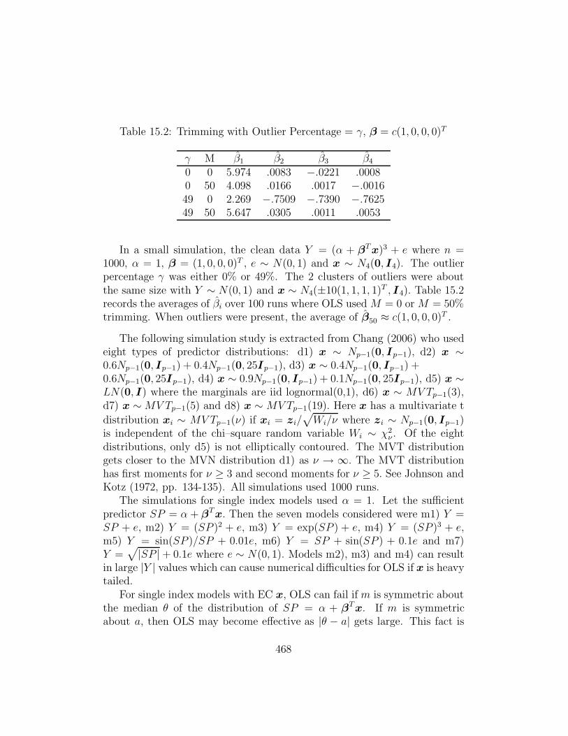
Table 15.2: Trimming with Outlier Percentage = γ, β = c(1, 0, 0, 0)T

γ M β1 β2 β3 β4

0 0 5.974 .0083 −.0221 .00080 50 4.098 .0166 .0017 −.001649 0 2.269 −.7509 −.7390 −.762549 50 5.647 .0305 .0011 .0053

In a small simulation, the clean data Y = (α + βT x)3 + e where n =1000, α = 1, β = (1, 0, 0, 0)T , e ∼ N(0, 1) and x ∼ N4(0, I4). The outlierpercentage γ was either 0% or 49%. The 2 clusters of outliers were aboutthe same size with Y ∼ N(0, 1) and x ∼ N4(±10(1, 1, 1, 1)T , I4). Table 15.2records the averages of βi over 100 runs where OLS used M = 0 or M = 50%trimming. When outliers were present, the average of β50 ≈ c(1, 0, 0, 0)T .

The following simulation study is extracted from Chang (2006) who usedeight types of predictor distributions: d1) x ∼ Np−1(0, Ip−1), d2) x ∼0.6Np−1(0, Ip−1) + 0.4Np−1(0, 25Ip−1), d3) x ∼ 0.4Np−1(0, Ip−1) +0.6Np−1(0, 25Ip−1), d4) x ∼ 0.9Np−1(0, Ip−1) + 0.1Np−1(0, 25Ip−1), d5) x ∼LN(0, I) where the marginals are iid lognormal(0,1), d6) x ∼ MV Tp−1(3),d7) x ∼ MV Tp−1(5) and d8) x ∼ MV Tp−1(19). Here x has a multivariate t

distribution xi ∼ MV Tp−1(ν) if xi = zi/√

Wi/ν where zi ∼ Np−1(0, Ip−1)is independent of the chi–square random variable Wi ∼ χ2

ν . Of the eightdistributions, only d5) is not elliptically contoured. The MVT distributiongets closer to the MVN distribution d1) as ν → ∞. The MVT distributionhas first moments for ν ≥ 3 and second moments for ν ≥ 5. See Johnson andKotz (1972, pp. 134-135). All simulations used 1000 runs.

The simulations for single index models used α = 1. Let the sufficientpredictor SP = α + βTx. Then the seven models considered were m1) Y =SP + e, m2) Y = (SP )2 + e, m3) Y = exp(SP ) + e, m4) Y = (SP )3 + e,m5) Y = sin(SP )/SP + 0.01e, m6) Y = SP + sin(SP ) + 0.1e and m7)Y =

√|SP | + 0.1e where e ∼ N(0, 1). Models m2), m3) and m4) can resultin large |Y | values which can cause numerical difficulties for OLS if x is heavytailed.

For single index models with EC x, OLS can fail if m is symmetric aboutthe median θ of the distribution of SP = α + βTx. If m is symmetricabout a, then OLS may become effective as |θ − a| gets large. This fact is

468

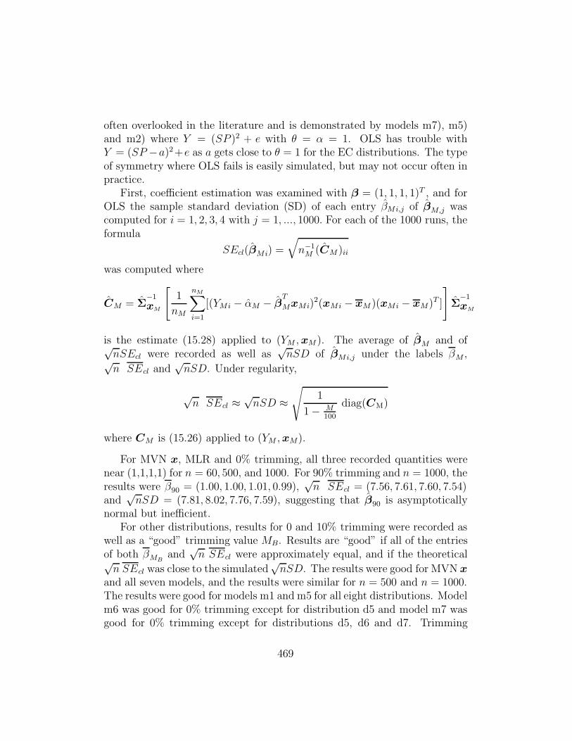
often overlooked in the literature and is demonstrated by models m7), m5)and m2) where Y = (SP )2 + e with θ = α = 1. OLS has trouble withY = (SP −a)2+e as a gets close to θ = 1 for the EC distributions. The typeof symmetry where OLS fails is easily simulated, but may not occur often inpractice.

First, coefficient estimation was examined with β = (1, 1, 1, 1)T , and forOLS the sample standard deviation (SD) of each entry βMi,j of βM,j wascomputed for i = 1, 2, 3, 4 with j = 1, ..., 1000. For each of the 1000 runs, theformula

SEcl(βMi) =

√n−1

M (CM )ii

was computed where

CM = Σ−1

xM

[1

nM

nM∑i=1

[(YMi − αM − βT

MxMi)2(xMi − xM )(xMi − xM)T ]

]Σ

−1

xM

is the estimate (15.28) applied to (YM , xM ). The average of βM and of√nSEcl were recorded as well as

√nSD of βMi,j under the labels βM ,√

n SEcl and√

nSD. Under regularity,

√n SEcl ≈

√nSD ≈

√1

1 − M100

diag(CM)

where CM is (15.26) applied to (YM , xM).

For MVN x, MLR and 0% trimming, all three recorded quantities werenear (1,1,1,1) for n = 60, 500, and 1000. For 90% trimming and n = 1000, theresults were β90 = (1.00, 1.00, 1.01, 0.99),

√n SEcl = (7.56, 7.61, 7.60, 7.54)

and√

nSD = (7.81, 8.02, 7.76, 7.59), suggesting that β90 is asymptoticallynormal but inefficient.

For other distributions, results for 0 and 10% trimming were recorded aswell as a “good” trimming value MB. Results are “good” if all of the entriesof both βMB

and√

n SEcl were approximately equal, and if the theoretical√n SEcl was close to the simulated

√nSD. The results were good for MVN x

and all seven models, and the results were similar for n = 500 and n = 1000.The results were good for models m1 and m5 for all eight distributions. Modelm6 was good for 0% trimming except for distribution d5 and model m7 wasgood for 0% trimming except for distributions d5, d6 and d7. Trimming

469

Table 15.3: OLS Coefficient Estimation with Trimming

m x M βM

√nSEcl

√nSD

m2 d1 0 2.00,2.01,2.00,2.00 7.81,7.79,7.76,7.80 7.87,8.00,8.02,7.88m5 d4 0 −.03,−.03,−.03,−.03 .30,.30,.30,.30 .31,.32,.33,.31m6 d5 0 1.04,1.04,1.04,1.04 .36,.36,.37,.37 .41,.42,.42,.40m7 d6 10 .11,.11,.11,.11 .58,.57,.57,.57 .60,.58,.62,.61

usually helped for models m2, m3 and m4 for distributions d5 – d8. Forn = 500, Table 15.3 shows that βM estimates cMβ and the average of theChen and Li (1998) SE is often close to the simulated SD.

Next testing was considered. Let FM denote the OLS statistic (15.30)applied to the nM cases (YM , xM) that remained after trimming. Ho wasrejected for OLS if FM > Fk,nM−p(0.95). Let p be the proportion of runswhere H0 was rejected. Since 1000 runs were used, the count 1000p ∼ bi-nomial(1000, 1 − δn) where 1 − δn converges to the true large sample level1 − δ. The standard error for the proportion is

√p(1 − p)/1000 ≈ 0.0069

for p = 0.05. An observed coverage p ∈ (0.03, 0.07) suggests that there is noreason to doubt that the true level is 0.05.

Suppose a 1D model holds but Y x. Then the Yi are iid and the modelreduces to Y = E(Y )+ e = cα + e where e = Y −E(Y ). As a special case, ifY = m(α+βT x)+e and if Y x, then Y = m(α)+e. For the correspondingtest H0 : β = 0 versus H1 : β �= 0, the OLS F statistic (15.30) is invariantwith respect to a constant. This test is interesting since if Ho holds, then theresults do not depend on the 1D model (15.1), but only on the distributionof x and the distribution of e. Since βOLS = cβ, power can be good ifc �= 0. The OLS test is equivalent to the ANOVA F test from MLR of Y onx. Under H0, the test should perform well provided that the design matrixis nonsingular and the error distribution and sample size are such that thecentral limit theorem holds. For the simulated data with β = 0, the modelis linear and normal, and the exact OLS level is 0.05 for n > p. Table 15.4illustrates this claim for n = 100 and n = 500.

Next the test Ho : β2 = 0 was considered. The OLS test is equivalent

470

Table 15.4: Rejection Proportions for H0: β = 0

x n F n Fd1 100 0.041 500 0.050d2 100 0.050 500 0.045d3 100 0.047 500 0.050d4 100 0.045 500 0.048d5 100 0.055 500 0.061d6 100 0.042 500 0.036d7 100 0.054 500 0.047d8 100 0.044 500 0.060

Table 15.5: Rejection Proportions for Ho: β2 = 0

m x 70 60 50 40 30 20 10 0 ADAP1 1 .061 .056 .062 .051 .046 .050 .044 .043 .0435 1 .019 .023 .019 .019 .020 .022 .027 .037 .0292 2 .023 .024 .026 .070 .183 .182 .142 .166 .0404 3 .027 .058 .096 .081 .071 .057 .062 .123 .1206 4 .026 .024 .030 .032 .028 .044 .051 .088 .0887 5 .058 .058 .053 .054 .046 .044 .051 .037 .0373 6 .021 .024 .019 .025 .025 .034 .080 .374 .0366 7 .027 .032 .023 .041 .047 .053 .052 .055 .055

471

to the t test from MLR of Y on x. The true model used α = 1 and β =

(1, 0, 1, 1)T . To simulate adaptive trimming, |corr(βT

Mx, βTx)| was computedfor M = 0, 10, ..., 90 and the initial trimming proportion MI maximized thiscorrelation. This process should be similar to choosing the best trimmed viewby examining 10 plots. The rejection proportions were recorded for M =0, ..., 90 and for adaptive trimming. The seven models, eight distributionsand sample sizes n = 60, 150, and 500 were used.

The test that used adaptive trimming had proportions ≤ 0.072 except formodel m4 with distributions d2, d3, d4, d6, d7 and d8; m2 with d4, d6 andd7 for n = 500 and d6 with n = 150; m6 with d4 and n = 60, 150; m5 withd7 and n = 500 and m7 with d7 and n = 500. With the exception of m4,when the adaptive p > 0.072, then 0% trimming had a rejection proportionnear 0.1. Occasionally adaptive trimming was conservative with p < 0.03.The 0% trimming worked well for m1 and m6 for all eight distributions andfor d1 and d5 for all seven models. Models m2 and m3 usually benefitedfrom adaptive trimming. For distribution d1, the adaptive and 0% trimmingmethods had identical p for n = 500 except for m3 where the values were0.038 and 0.042. Table 15.5 used n = 150 and supports the claim that theadaptive trimming estimator can be asymptotically equivalent to OLS (0%trimming) and that trimming can greatly improve the type I error.

15.6 Complements

For 1D regression models, suppose that |corr(βT

OLSx, βTx)| ≥ 0.95 where β

is a good estimator of dβ for d �= 0, or that the 1D regression can be visualizedwith the OLS response plot. For example, the plotted points cluster tightlyabout the mean function m. Then OLS should be a useful 1D estimatorand output originally meant for MLR is also often useful for 1D regression(1DR) data. In particular, i) βOLS estimates β for MLR and cβ for 1DR.ii) The F test statistics tend to have a χ2

k/k limiting distribution for MLR,and the Fk,n−p cutoffs tend to be useful for exploratory purposes for 1DR. iii)Variable selection with the Cp statistic is effective. iv) The MSE estimatesσ2 for MLR and τ 2 for 1DR. v) The OLS response plot is a very effectivetool for visualizing the regression and outlier detection. The estimated meanfunction for MLR is the unit slope line through the origin, but tends to benonlinear for 1DR. vi) Resistant

√n consistent estimators based on OLS and

ellipsoidal trimming exist for both MLR and 1DR. vii) Cook’s distance is a

472

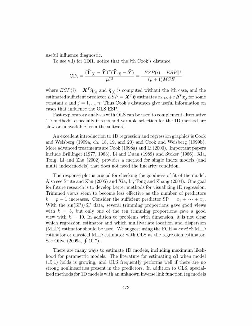
useful influence diagnostic.To see vii) for 1DR, notice that the ith Cook’s distance

CDi =(Y (i) − Y )T (Y (i) − Y )

pσ2=

‖ESP (i) − ESP‖2

(p + 1)MSE

where ESP (i) = XT η(i) and η(i) is computed without the ith case, and the

estimated sufficient predictor ESP = XT η estimates αOLS+c βTxj for someconstant c and j = 1, ..., n. Thus Cook’s distances give useful information oncases that influence the OLS ESP.

Fast exploratory analysis with OLS can be used to complement alternative1D methods, especially if tests and variable selection for the 1D method areslow or unavailable from the software.

An excellent introduction to 1D regression and regression graphics is Cookand Weisberg (1999a, ch. 18, 19, and 20) and Cook and Weisberg (1999b).More advanced treatments are Cook (1998a) and Li (2000). Important papersinclude Brillinger (1977, 1983), Li and Duan (1989) and Stoker (1986). Xia,Tong, Li and Zhu (2002) provides a method for single index models (andmulti–index models) that does not need the linearity condition.

The response plot is crucial for checking the goodness of fit of the model.Also see Stute and Zhu (2005) and Xia, Li, Tong and Zhang (2004). One goalfor future research is to develop better methods for visualizing 1D regression.Trimmed views seem to become less effective as the number of predictorsk = p − 1 increases. Consider the sufficient predictor SP = x1 + · · · + xk.With the sin(SP)/SP data, several trimming proportions gave good viewswith k = 3, but only one of the ten trimming proportions gave a goodview with k = 10. In addition to problems with dimension, it is not clearwhich regression estimator and which multivariate location and dispersion(MLD) estimator should be used. We suggest using the FCH = covfchMLDestimator or classical MLD estimator with OLS as the regression estimator.See Olive (2009a,

∮10.7).

There are many ways to estimate 1D models, including maximum likeli-hood for parametric models. The literature for estimating cβ when model(15.1) holds is growing, and OLS frequently performs well if there are nostrong nonlinearities present in the predictors. In addition to OLS, special-ized methods for 1D models with an unknown inverse link function (eg models

473

(15.2) and (15.3)) have been developed, and often the focus is on develop-ing asymptotically efficient methods. See the references in Cavanagh andSherman (1998), Delecroix, Hardle and Hristache (2003), Hardle, Hall andIchimura (1993), Horowitz (1998), Hristache, Juditsky, Polzehl, and Spokoiny(2001), Stoker (1986), Weisberg and Welsh (1994), Xia (2006) and Xia, Tong,Li and Zhu (2002).

Some of these methods standardize β so β1 = 1. This standardizationmay cause problems for testing β = 0 and β1 = 0.

Several papers have suggested that outliers and strong nonlinearities needto be removed from the predictors. See Brillinger (1991), Cook (1998a, p.152), Cook and Nachtsheim (1994) and Li and Duan (1989, p. 1011, 1041,1042). Trimmed views were introduced by Olive (2002, 2004b). Li, Cookand Nachtsheim (2004) find clusters, fit OLS to each cluster and then poolthe OLS estimators into a final estimator. This method uses all n caseswhile trimmed views gives M% of the cases weight zero. The trimmed viewsestimator will often work well when outliers and influential cases are present.

Section 15.4 follows Olive and Hawkins (2005) closely. The literatureon numerical methods for variable selection in the OLS multiple linear re-gression model is enormous, and the literature for other given 1D regressionmodels is also growing. Li, Cook and Nachtsheim (2005) give an alternativemethod for variable selection that can work without specifying the model.Also see, for example, Claeskins and Hjort (2003), Efron, Hastie, Johnstoneand Tibshirani (2004), Fan and Li (2001, 2002), Hastie (1987), Kong andXia (2007), Lawless and Singhai (1978), Leeb and Potscher (2006), Naik andTsai (2001), Nordberg (1982) and Tibshirani (1996). For generalized linearmodels, forward selection and backward elimination based on the AIC crite-rion are often used. See Chapters 11, 12 and 13, Agresti (2002, p. 211-217),Cook and Weisberg (1999a, p. 485, 536-538). Again, if the variable selectiontechniques in these papers are successful, then the estimated sufficient pre-dictors from the full and candidate model should be highly correlated, andthe EE, VV and response plots will be useful. Survival regression modelsalso use AIC. See Chapter 16.

The variable selection model with x = (xTS , xT

E)T and SP = α + βT x =α + βT

SxS is not the only variable selection model. Burnham and Anderson(2004) note that for many data sets, the variables can be ordered in decreasing

474

importance from x1 to xp−1. The “tapering effects” are such that if n >> p,then all of the predictors should be used, but for moderate n it is better todelete some of the least important predictors.

Section 15.5 followed Chang and Olive (2010) closely. More examplesand simulations are in Chang (2006). Severini (1998) discusses when OLSoutput is relevant for the Gaussian additive error single index model. Li andDuan (1989) and Li (1997) suggest that OLS F tests are asymptotically validif x is multivariate normal and if βOLS = Σ−1

x ΣxY �= 0. Freedman (1981),

Brillinger (1983) and Chen and Li (1998) also discuss Cov(βOLS). Formaltesting procedures for the single index model are given by Simonoff and Tsai(2002) and Gao and Liang (1997). Chang and Olive (2007) shows how toapply ellipsoidal trimming to general 1D methods, including OLS.

The mussel data set is included as the file mussel.lsp in the Arc softwareand can be obtained from the web site (http://www.stat.umn.edu/arc/).The Boston housing data can be obtained from the text website or from theSTATLIB website (http://lib.stat.cmu.edu/datasets/boston).

15.7 Problems

15.1. Refer to Definition 15.3 for the Cox and Snell (1968) definition forresiduals, but replace η by β.

a) Find ei if Yi = µ + ei and T (Y ) is used to estimate µ.b) Find ei if Yi = xT

i β + ei.c) Find ei if Yi = β1 exp[β2(xi − x)]ei where the ei are iid exponential(1)

random variables and x is the sample mean of the x′is.

d) Find ei if Yi = xTi β + ei/

√wi.

15.2∗. (Aldrin, Bφlviken, and Schweder 1993). Suppose

Y = m(βTx) + e (15.35)

where m is a possibly unknown function and the zero mean errors e are inde-pendent of the predictors. Let z = βTx and let w = x −E(x). Let Σx,Y =Cov(x, Y ), and let Σx =Cov(x) = Cov(w). Let r = w − (Σxβ)βT w.

a) Recall that Cov(x, Y ) = E[(x − E(x))(Y − E(Y ))T ] and show thatΣx,Y = E(wY ).

475

b) Show that E(wY ) = Σx,Y = E[(r + (Σxβ)βT w) m(z)] =

E[m(z)r] + E[βT w m(z)]Σxβ.

c) Using βOLS = Σ−1x Σx,Y , show that βOLS = c(x)β + u(x) where the

constantc(x) = E[βT (x − E(x))m(βTx)]

and the bias vector u(x) = Σ−1x E[m(βT x)r].

d) Show that E(wz) = Σxβ. (Hint: Use E(wz) = E[(x−E(x))xTβ] =E[(x− E(x))(xT − E(xT ) + E(xT ))β].)

e) Assume m(z) = z. Using d), show that c(x) = 1 if βT Σxβ = 1.

f) Assume that βTΣxβ = 1. Show that E(zr) = E(rz) = 0. (Hint: FindE(rz) and use d).)

g) Suppose that βT Σxβ = 1 and that the distribution of x is multivariatenormal. Then the joint distribution of z and r is multivariate normal. Usingthe fact that E(zr) = 0, show Cov(r, z) = 0 so that z and r are independent.Then show that u(x) = 0.

(Note: the assumption βT Σxβ = 1 can be made without loss of gen-erality since if βTΣxβ = d2 > 0 (assuming Σx is positive definite), theny = m(d(β/d)T x) + e ≡ md(η

T x) + e where md(u) = m(du), η = β/d andηTΣxη = 1.)

15.3. Suppose that you have a statistical model where both fitted valuesand residuals can be obtained. For example this is true for time series andfor nonparametric regression models such as Y = f(x1, ..., xp) + e where

y = f(x1, ..., xp) and the residual e = Y − f(x1, ..., xp). Suggest graphs forvariable selection for such models.

476

Output for Problem 15.4.

BEST SUBSET REGRESSION MODELS FOR CRIM

(A)LogX2 (B)X3 (C)X4 (D)X5 (E)LogX7 (F)X8 (G)LogX9 (H)LogX12

3 "BEST" MODELS FROM EACH SUBSET SIZE LISTED.

ADJUSTED

k CP R SQUARE R SQUARE RESID SS MODEL VARIABLES

-- ----- -------- -------- --------- ---------------

1 379.8 0.0000 0.0000 37363.2 INTERCEPT ONLY

2 36.0 0.3900 0.3913 22744.6 F

2 113.2 0.3025 0.3039 26007.8 G

2 191.3 0.2140 0.2155 29310.8 E

3 21.3 0.4078 0.4101 22039.9 E F

3 25.0 0.4036 0.4059 22196.7 F H

3 30.8 0.3970 0.3994 22442.0 D F

4 17.5 0.4132 0.4167 21794.9 C E F

4 18.1 0.4125 0.4160 21821.0 E F H

4 18.8 0.4117 0.4152 21850.4 A E F

5 10.2 0.4226 0.4272 21402.3 A E F H

5 10.8 0.4219 0.4265 21427.7 C E F H

5 12.0 0.4206 0.4252 21476.6 A D E F

6 5.7 0.4289 0.4346 21125.8 A C E F H

6 9.3 0.4248 0.4305 21279.1 A C D E F

6 10.3 0.4237 0.4294 21319.9 A B E F H

7 6.3 0.4294 0.4362 21065.0 A B C E F H

7 6.3 0.4294 0.4362 21066.3 A C D E F H

7 7.7 0.4278 0.4346 21124.3 A C E F G H

8 7.0 0.4297 0.4376 21011.8 A B C D E F H

8 8.3 0.4283 0.4362 21064.9 A B C E F G H

8 8.3 0.4283 0.4362 21065.8 A C D E F G H

9 9.0 0.4286 0.4376 21011.8 A B C D E F G H

15.4. The output above is for the Boston housing data from softwarethat does all subsets variable selection. The full model is a 1D transformationmodel with response variable Y = CRIM and uses a constant and variablesA, B, C, D, E, F, G and H. (Using log(CRIM) as the response would give anMLR model.) From this output, what is the best submodel? Explain briefly.

477

15.5∗. a) Show that Cp(I) ≤ 2k if and only if FI ≤ p/(p − k).

b) Using (15.19), find E(Cp) and Var(Cp) assuming that an MLR modelis appropriate and that Ho (the reduced model I can be used) is true.

c) Using (15.19), Cp(Ifull) = p and the notation in Section 15.4, showthat

Cp(Ii) = Cp(Ifull) + (t2i − 2).

R/Splus Problems

Warning: Use the command source(“A:/regpack.txt”) to downloadthe programs. See Preface or Section 17.2. Typing the name of theregpack function, eg trviews, will display the code for the function. Use theargs command, eg args(trviews), to display the needed arguments for thefunction.

15.6. Use the following R/Splus commands to make 100 N3(0, I3) casesand 100 trivariate non-EC cases.

n3x <- matrix(rnorm(300),nrow=100,ncol=3)

ln3x <- exp(n3x)

In R, type the command library(MASS).

a) Using the commands pairs(n3x) and pairs(ln3x) and include both scat-terplot matrices in Word. (Click on the plot and hit Ctrl and c at the sametime. Then go to file in the Word menu and select paste.) Are strongnonlinearities present among the MVN predictors? How about the non-ECpredictors? (Hint: a box or ball shaped plot is linear.)

b) Make a single index model and the sufficient summary plot with thefollowing commands

ncy <- (n3x%*%1:3)^3 + 0.1*rnorm(100)

plot(n3x%*%(1:3),ncy)

and include the plot in Word.c) The command trviews(n3x, ncy) will produce ten plots. To advance the

plots, click on the rightmost mouse button (and in R select stop) to advanceto the next plot. The last plot is the OLS view. Include this plot in Word.

478

d) After all 10 plots have been looked at the output will show 10 estimatedpredictors. The last estimate is the OLS (least squares) view and might looklike

Intercept X1 X2 X3

4.417988 22.468779 61.242178 75.284664

If the OLS view is a good estimated sufficient summary plot, then theplot created from the command (leave out the intercept)

plot(n3x%*%c(22.469,61.242,75.285),n3x%*%1:3)

should cluster tightly about some line. Your linear combination will be dif-ferent than the one used above. Using your OLS view, include the plot usingthe command above (but with your linear combination) in Word. Was thisplot linear? Did some of the other trimmed views seem to be better thatthe OLS view, that is, did one of the trimmed views seem to have a smoothmean function with a smaller variance function than the OLS view?

e) Now type the R/Splus command

lncy <- (ln3x%*%1:3)^3 + 0.1*rnorm(100).

Use the command trviews(ln3x,lncy) to find the best view with a smoothmean function and the smallest variance function. This view should not bethe OLS view. Include your best view in Word.

f) Get the linear combination from your view, say (94.848, 216.719, 328.444)T ,and obtain a plot with the command

plot(ln3x%*%c(94.848,216.719,328.444),ln3x%*%1:3).

Include the plot in Word. If the plot is linear with high correlation, thenyour response plot in e) should be good.

15.7. (At the beginning of your R/Splus session, use thesource(“A:/regpack.txt”) command (and library(MASS) in R.))

a) Perform the commands

> nx <- matrix(rnorm(300),nrow=100,ncol=3)

> lnx <- exp(nx)

> SP <- lnx%*%1:3

> lnsincy <- sin(SP)/SP + 0.01*rnorm(100)

479

For parts b), c) and d) below, to make the best trimmed view withtrviews, ctrviews or lmsviews, you may need to use the function twice.The first view trims 90% of the data, the next view trims 80%, etc. The lastview trims 0% and is the OLS view (or lmsreg view). Remember to advancethe view with the rightmost mouse button (and in R, highlight “stop”). Thenclick on the plot and next simultaneously hit Ctrl and c. This makes a copyof the plot. Then in Word, use the menu commands “Copy>paste.”

b) Find the best trimmed view with OLS and covfch with the followingcommands and include the view in Word.

> trviews(lnx,lnsincy)

(With trviews, suppose that 40% trimming gave the best view. Theninstead of using the procedure above b), you can use the command

> essp(lnx,lnsincy,M=40)

to make the best trimmed view. Then click on the plot and next simultane-ously hit Ctrl and c. This makes a copy of the plot. Then in Word, use themenu commands “Copy>paste”. Click the rightmost mouse button (and inR, highlight “stop”) to return the command prompt.)

c) Find the best trimmed view with OLS and (x, S) using the followingcommands and include the view in Word. See the paragraph above b).

> ctrviews(lnx,lnsincy)

d) Find the best trimmed view with lmsreg and cov.mcd using the fol-lowing commands and include the view in Word. See the paragraph aboveb).

> lmsviews(lnx,lnsincy)

e) Which method or methods gave the best response plot? Explain briefly.

480