HEC-RAS: 1D VS 2DA COMPARISON OF MODELING RESULTS

Presented By:Wesley “Ross” Perry, PE CFM

What Is HEC-RAS?

Hydrologic

Engineering

Center -

River

Analysis

System

1995 – HEC-RAS V1.0◦ 1D Steady Flow

2006 – HEC-RAS V4.0◦ 1D Unsteady Flow

2016 – HEC-RAS V5.0◦ 2D Unsteady Flow

June 2018 – HEC-RAS V5.0.5

History

➢Powerful Computer Software Used Worldwide

➢Hydraulic Modeling of Water Flow Through Rivers and Other Channels◦ 1D Steady Flow Hydraulics

◦ 1D & 2D Unsteady Flow Hydraulics

◦ Sediment Transport-Mobile Bed Modeling

◦ Water Temperature Analysis

◦ Water Quality Modeling

All Using a Common Geometric Data Representation

It’s FREE!

Subcritical, Supercritical, Mixed Flow

HEC-RAS Today

1D Model Calculations

How Does It Work – 1D Models

One Dimension (1D)

Discharge & Velocities Calculated for One Dimension Only➢Vector Along Channel Slope

➢Perpendicular to Cross Sections

How Does It Work – 1D Models

0.2

0.1

0.0

Steady Flow Example from Chapter 4 Plan: Existing Conditions Run 9/6/2018

Legend

WS 10 yr

Ground

Bank Sta

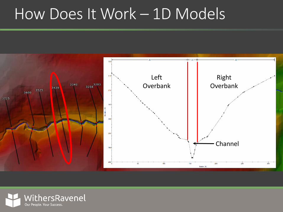
How Does It Work – 1D Models

LeftOverbank

RightOverbank

Channel

Downstream Boundary Conditions➢Known WSE (Tailwater Condition)

➢Normal Depth (Slope)

➢Critical Depth

➢Flow / Stage Hydrograph

➢Rating Curve

How Does It Work – 1D Models

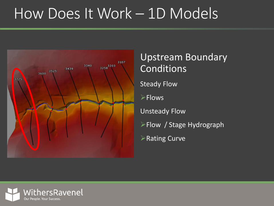
Upstream Boundary Conditions

Steady Flow

➢Flows

Unsteady Flow

➢Flow / Stage Hydrograph

➢Rating Curve

How Does It Work – 1D Models

Standard Step Method(Conservation of Mass & Energy)

0.2

0.1

0.0

Steady Flow Example from Chapter 4 Plan: Existing Conditions Run 9/6/2018

Legend

WS 10 yr

Ground

Bank Sta

𝑍2 + 𝑌2 +α2𝑉2

2

2𝑔+= 𝑍1 + 𝑌1 +

α1𝑉12

2𝑔+ ℎ𝑒

Potential Energy

Kinetic Energy

How Does It Work – 1D Models

Losses

𝑉 = ൗ𝑄 𝐴

Energy Losses

ℎ𝑒 = 𝐿𝑆𝑓 + 𝐶α2𝑉2

2

2𝑔−

α1𝑉12

2𝑔

𝑛𝑐 =σ𝑖=1𝑁 (𝑃𝑖𝑛𝑖

1.5)

𝑃

2/3

Friction Losses – Manning’s EquationComposite “n” Value:

Contraction & Expansion(User Defined)

How Does It Work – 1D Models

Computation Procedure

Iterative Process

➢Determine Downstream WSE

➢Assume WSE for Upstream XS

➢Solve for Conveyance & Velocity Head

➢Calculate Friction Slope and Solve for Energy Losses

➢Solve Energy Equation for Upstream WSE

➢Compare (Difference >0.01 ft?)

How Does It Work – 1D Models

Mixed Flow Regimes𝐹𝑛 =

𝑉

(𝑔𝐴𝐵)0.5

Froude Number

<1 = Subcritical Flow

>1 = Supercritical Flow

Supercritical Flow

Subcritical Flow

Hydraulic Jump

How Does It Work – 1D Models

Other Equations➢ Momentum Equations➢ Bridge Hydraulics

➢ Expansion Reach Length & Rate Equations➢ Contraction Reach Length & Rate Equations➢ Pressure & Weir Flow Equations➢ Yarnell/Pier Equations

➢ Culvert Hydraulics➢ Orifice & Weir Flow Equations➢ Inlet and Outlet Control Equations➢ Losses (Entrance, Exit, Friction, Etc…)

How Does It Work – 1D Models

1D HEC-RAS Model – Isometric View

2D Models Calculations

How Does It Work – 2D Models

Two Dimension (2D)

Discharge & Velocities Calculated for Two Dimensions➢X & Y Directions at Each Cell Face➢Allows for lateral and upstream flows

How Does It Work – 2D Models

1D

1D vs 2D Models

2D

How Does It Work – 2D Models

2D Flow Area

How Does It Work – 2D Models

2D Flow Area – Flexible Mesh

Single Cell

Elevation

X

Y

Top View

Large Cells Retain Underlying Terrain Details

How Does It Work – 2D Models

How Does It Work – 2D Models

Manning’s ValuesLand Cover Layer

➢Each Color Represents Different “n” Value

➢“n” Value Assigned to Each Cell Face

How Does It Work – 2D Models

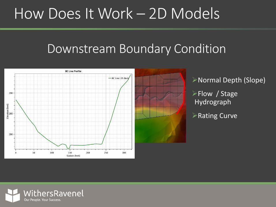
Downstream Boundary Condition

➢Normal Depth (Slope)

➢Flow / Stage Hydrograph

➢Rating Curve

How Does It Work – 2D Models

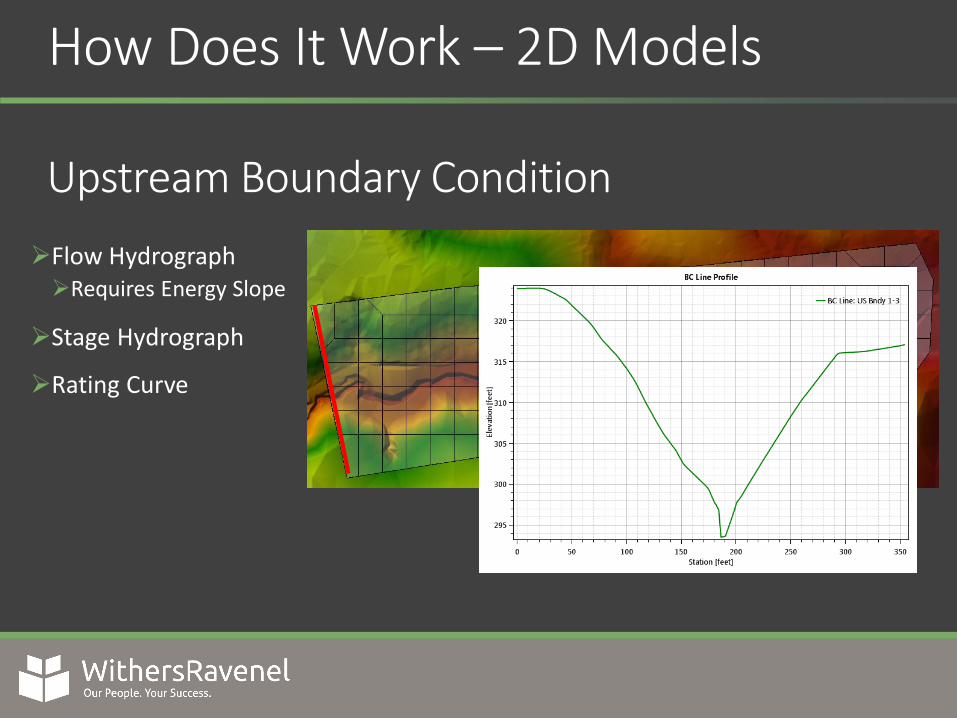
Upstream Boundary Condition

➢Flow Hydrograph➢Requires Energy Slope

➢Stage Hydrograph

➢Rating Curve

How Does It Work – 2D Models

Calculations: Full St. Venant (Full Momentum)

1

𝐴

δ𝑄

δ𝑡+1

𝐴

δ

δ𝑥

𝑄

𝐴

2

+ gδ𝑦

δ𝑥− 𝑔 𝑆𝑜 − 𝑆𝑓 = 0

Inertia Diffusive Wave

LocalAccel.

ConvectiveAccel.

PressureGradient

Gravity Friction

How Does It Work – 2D Models

COMPARISON OF RESULTSSingle Channel

1D Model 2D Model

Comparison: Single Channel

1D & 2D Model Inputs – Geometry

1D Model Cross Section 2D Model Profile Along Same Alignment

Comparison: Single Channel

1D & 2D Model Inputs – Geometry & Manning’s

Comparison: Single Channel

100-Yr, 24-HrPeak Flow = 680 cfs

1D & 2D Model Inputs – Boundary Conditions

Downstream Boundary ConditionNormal Depth: Slope = 0.005 ft/ft

Single Channel

Cross Section1D

Max WSE2D

Max WSEDifference

3600 296.01 296.45 0.44

3525 294.59 295.76 1.17

3439 293.12 293.75 0.63

3340 291.74 292.82 1.08

3258 290.55 292.81 2.26

3203 289.86 290.46 0.60

3107 288.90 289.69 0.79

3017 287.75 287.95 0.20

2858 285.76 286.34 0.58

2758 284.79 285.28 0.49

2658 284.23 284.51 0.28

2525 283.56 283.75 0.19

2435 282.29 282.45 0.16

2281 280.15 280.22 0.07

2211 279.56 279.22 -0.34

Maximum Difference (ft): 2.26

Average Difference (ft): 0.57

Comparison: Single Channel

2D Model

1D Model

1D WSE Profile

2D WSE Profile

Topographic Surface

COMPARISON OF RESULTSMultiple Channels

Peak Flow = 363 cfs

Peak Flow = 680 cfs

Peak Flow = 503 cfs Peak Flow = 170 cfs

Comparison: Multi Channels

1D Model Downstream Boundary ConditionNormal Depth: Slope = 0.005 ft/ft

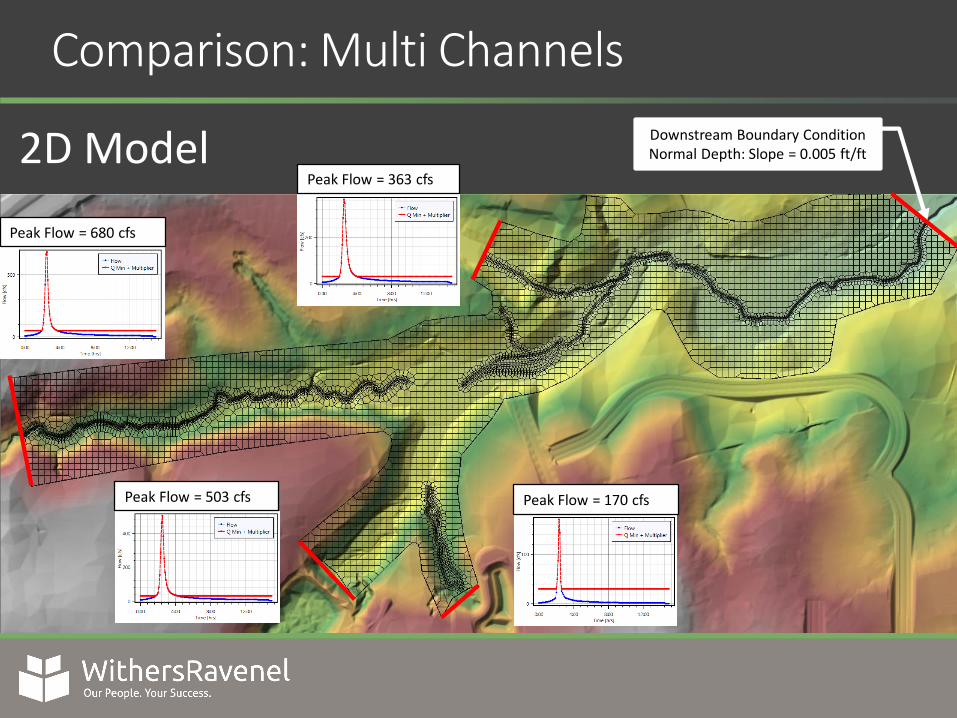
Comparison: Multi Channels

2D ModelPeak Flow = 363 cfs

Peak Flow = 680 cfs

Peak Flow = 503 cfs Peak Flow = 170 cfs

Downstream Boundary ConditionNormal Depth: Slope = 0.005 ft/ft

Multiple Channels

Maximum Difference (ft): 1.72

Average Difference (ft): 1.47

2D Model

1D Model

Comparison: Multi Channels

1D WSE Profile

2D WSE Profile

Topographic Surface

COMPARISON OF RESULTSMultiple Channels w/ Crossings

Comparison: Multi Channels w/ Crossings

1D Model

Geometry & Boundary Conditions➢ Same Geometry as Previous

+ Crossings+ Ineffective Flow Areas

➢ Same Flows (100-Yr, 24Hr)

Comparison: Multi Channels w/ Crossings

Channel Culvert• 72” RCPOverbank Culvert• 60” RCP

Channel Culvert• 84” RCPOverbank Culvert• 3 - 72” RCP

40’ Bridge Span• 6’ Wide Pier

Comparison: Multi Channels w/ Crossings

2D Model

Culvert Crossings Similar to 1DCulverts Discharge to Adjacent CellFaces Instead of Cross Sections

Bridge Crossings Bridge Abutments & PierConveyance ObstructionsUsed to Alter Terrain

Comparison: Multi Channels w/ Crossings

Max WSE Results

2D Model

1D Model

Comparison: Multi Channels w/ Crossings

2D Model

1D Model

Multiple Channels w/ Crossings

Maximum Difference (ft): 3.50

Average Difference (ft): 1.18

1D WSE Profile

2D WSE Profile

Topography Surface

Culvert Crossing

Comparison: Multi Channels w/ Crossings

2D Model

1D Model Multiple Channels w/ Crossings

Maximum Difference (ft): 0.64

Average Difference (ft): 0.33

1D WSE Profile

2D WSE Profile

1D Topography Surface

Culvert Crossing

2D Topography Surface

Comparison: Multi Channels w/ Crossings

2D Model

1D Model

Multiple Channels w/ Crossings

Maximum Difference (ft): 1.44

Average Difference (ft): 0.37

1D WSE Profile

2D WSE Profile2D Topography Surface

(Bridge Pier)

Bridge Crossing

1D Topography Surface

COMPARISON OF RESULTSCascading Dam Failure

Comparison: Cascading Dam Failure

1D Model

Geometry & Boundary Conditions➢ Same Geometry as Previous

+ Inline Structures (Dams)+ Upper Pond (Storage Area)+ Lower Pond (HD Cross Sections)

➢ Same Flows (100-Yr, 24Hr)

Upper Pond

Lower Pond

Comparison: Cascading Dam FailureUpper Dam

Lower Dam

Upper Pond – Storage Area

Breach Parameters – Froehlich (1995a)Initial WSE = Spillway CrestDam Breach at Peak of Inflow Hydrograph

Breach Parameters – Froehlich (1995a)Initial WSE = Spillway CrestDam Breach Once Dam is Overtopped

Upper Pond

Lower Pond

Comparison: Cascading Dam Failure

2D Model

Upper Pond(Storage Area)

Lower Pond(Flow Area) Geometry & Boundary Conditions

➢ Same Geometry as Previous+ 2D/SA Connections (Dams)+ Upper Pond (Storage Area)+ Lower Pond (2D Flow Area)

➢ Same Flows (100-Yr, 24Hr)

Comparison: Cascading Dam Failure

2D Model

1D Model

Comparison: Cascading Dam Failure

2D Model

1D Model

Cascading Dam Breach

Maximum Difference (ft): 2.83

Average Difference (ft): 0.94

1D WSE Profile

2D WSE Profile

Topography Surface

Culvert Crossing

Comparison: Cascading Dam Failure

Cascading Dam Breach

Maximum Difference (ft): 0.89

Average Difference (ft): 0.66

2D Model

1D Model

1D WSE Profile

2D WSE Profile1D Topography Surface

Culvert Crossing

2D Topography Surface

Comparison: Cascading Dam Failure

Cascading Dam Breach

Maximum Difference (ft): 2.94

Average Difference (ft): 1.46

2D Model

1D Model

1D WSE Profile

2D WSE Profile

2D Topography Surface(Bridge Pier)

Bridge Crossing

1D Topography Surface

Lower Dam

Comparison: Cascading Dam Failure

1D Dam Breach Model

2D Dam Breach Model

ASSESSMENT OF RESULTS

Areas of Interest

Multiple Channels with Crossings

Well Defined ChannelRelatively Steep (0.01 ft/ft)

Why the Difference in Results?

1D Model - Velocity

2D Model - Velocity

Areas of Interest

Multiple Channels with CrossingsLarge Bend in Floodplain

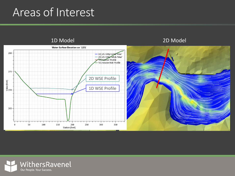
Areas of Interest

2D Model1D Model

1D WSE Profile

2D WSE Profile

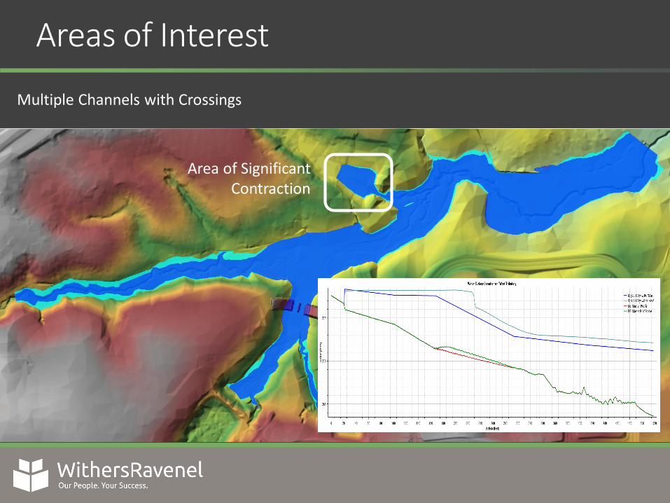
Areas of Interest

Multiple Channels with Crossings

Area of Significant Contraction

Areas of Interest

1D Model 2D Model

Lessons Learned

Pros of 2D vs 1D➢ Unsteady Models Are More Stable➢ Faster Model Build Time➢ Less Subjective Decisions

➢ Ineffective Flow Areas➢ Contraction/Expansion Ratios➢ Cross Section Locations & Spacing

➢ High Resolution Flow Characteristics➢ Velocity➢ Shear Stress➢ Stream Power

➢ Accounts for Inertia➢ Eddies, Super Elevation, etc.

➢ Cool Hydrodynamic Animations!

Cons of 2D vs 1D➢ Need Detailed Topography

➢ Additional Software May be Needed➢ Not Warranted for Small Projects

➢ Longer Run Times➢ No Bridge Hydraulic Structures➢ No Scour Analysis➢ No Pump Stations

When Should You Use 1D Models?

➢ Standard Channel Flows➢ Mostly Uni-Directional Flow➢ Minimal Lateral Expansion/Contraction➢ Relatively Shallow Slopes

➢ FEMA➢ CLOMR/LOMRs➢ No-Rise Flood Studies

➢ Reviewers Request

➢ Bridge Design/Scour Analysis/Channel Stabilization

➢ Pump Stations

➢ Small, Quick Projects➢ Ex: Backwater Elevations

When Should You Use 2D Models?

➢ Anywhere with Detailed Terrain Data

➢ Large Flat Floodplains

➢ No Defined Channel (Flow Path is Uncertain)➢ Alluvial Fans & Estuaries➢ Multiple Flow Paths

➢ Large Meandering Streams

➢ Lateral Flows

➢ High Resolution Hydraulics Around Obstructions

➢ Velocity, Shear Stress, Depth x Velocity

OR….

Mix it Up – 1D & 2D Models

Thank You!

Questions?