hec-ras 1d unsteady flow modeling guidelines
TRANSCRIPT
HEC-RAS 1D UNSTEADY FLOW
MODELING GUIDELINES
June 2019

HEC-RAS 1D Unsteady Flow Modeling Guidelines June 2019 i
Table of Contents
SECTION 1 - INTRODUCTION ........................................................................................1
1.1 Preface..........................................................................................................1 1.2 Application of HEC-RAS Unsteady Flow ...................................................1
SECTION 2 - BOUNDARY CONDITIONS ......................................................................3
2.1 Introduction ..................................................................................................3 2.2 External Boundary Conditions .....................................................................3 2.2.1 Upstream Boundary Conditions ...................................................................4 2.2.2 Downstream Boundary Conditions ..............................................................5 2.3 Internal Boundary Conditions ......................................................................7 2.3.1 Lateral Inflow Hydrographs .........................................................................8 2.3.2 Uniform Lateral Inflow Hydrographs ..........................................................9 2.3.3 Internal Boundary Condition Rating Curves .............................................12 2.3.4 Internal Boundary Condition Stage Hydrographs......................................12 2.4 Minimum Flows .........................................................................................12 2.5 Initial Conditions .......................................................................................12 2.5.1 Initial Flows ...............................................................................................13 2.5.2 Initial Stages...............................................................................................13
SECTION 3 - COMPUTATION OPTIONS .....................................................................14
3.1 General Options .........................................................................................14 3.2 Friction Slope Methods ..............................................................................14 3.3 Mixed Flow ................................................................................................14 3.4 Computation Intervals ................................................................................14 3.5 Advanced Time Step Control.....................................................................15
SECTION 4 - GEOMETRY ..............................................................................................16
4.1 Introduction ................................................................................................16 4.2 Cross-sections ............................................................................................16 4.2.1 HTAB .........................................................................................................16 4.2.2 Reach Lengths ............................................................................................16 4.2.3 Obstructions ...............................................................................................17 4.2.4 Ineffective Flow .........................................................................................18 4.2.5 Contraction and Expansion Coefficients ...................................................20 4.2.6 Pilot Channels ............................................................................................20 4.2.7 Lidded Cross-sections ................................................................................22 4.3 Bridge and Culvert Structures ....................................................................22 4.3.1 Options .......................................................................................................22
HEC-RAS 1D Unsteady Flow Modeling Guidelines June 2019 ii
4.3.2 HTAB .........................................................................................................25 4.3.3 Bridge Modeling Approach .......................................................................26 4.4 Inline Weirs ................................................................................................26 4.5 Lateral Structures .......................................................................................27 4.6 Storage Areas .............................................................................................31 4.6.1 Storage Area Connectors ...........................................................................33 4.7 Junctions ....................................................................................................33 4.8 Levees ........................................................................................................35
SECTION 5 - MODEL DEBUGGING .............................................................................37
5.1 Data Quality ...............................................................................................37 5.2 Cross-Sections............................................................................................37 5.2.1 Common Sources of Instability .................................................................37 5.2.2 Common Data Issues .................................................................................39 5.3 Start-Up and Low Flows ............................................................................39 5.4 High Flows .................................................................................................40 5.5 Reviewing Results .....................................................................................41 5.6 Restart Files and Computed Profiles..........................................................42
SECTION 6 - CONVERTING UNSTEADY FLOW TO STEADY FLOW ....................44
SECTION 7 - MODEL OUTPUTS & DELIVERABLES ................................................51
7.1 Model Files ................................................................................................53 7.2 Boundary Conditions .................................................................................56 7.3 Additional Model Details ...........................................................................63

HEC-RAS 1D Unsteady Flow Modeling Guidelines June 2019 iii
Figure 2-1 - Upstream Flow Boundary Condition .............................................................. 4 Figure 2-2 - Internal Lateral Inflow Boundary Condition (K142A) ................................... 8 Figure 2-3 - Internal Uniform Lateral Inflow Boundary Condition (K142A) .................... 9 Figure 2-4 - Internal Uniform Lateral Inflow Boundary Condition (K142B) .................. 10 Figure 2-5 - Boundary Condition Overview (K142) ........................................................ 11 Figure 2-2-6 - Initial Flow Assignment at Flow Split ....................................................... 13 Figure 4-1 - Overbank Volume ......................................................................................... 17 Figure 4-2 - Example of Obstructed Area Modeled as Storage Area ............................... 17 Figure 4-3 - Single Ineffective Flow Area ........................................................................ 18 Figure 4-4 - Multiple Blocked Ineffective Areas - To Reflect Geometry ........................ 19 Figure 4-5 - Example of Multiple Blocked Ineffective Areas - For Stability ................... 19 Figure 4-6 - Example of a Pilot Channel (Profile View) .................................................. 21 Figure 4-7 - Example of a Pilot Channel (Cross-section View) ....................................... 21 Figure 4-8 - Skew Angle for Oblique Abutments ............................................................. 24 Figure 4-9 - Skew Angle for Parallel Abutments ............................................................. 24 Figure 4-10 - Example of Variable Skew ......................................................................... 24 Figure 4-11 - Inline Weir Added for Stability .................................................................. 26 Figure 4-12 - Example of Lateral Structures at Bridges ................................................... 28 Figure 4-13 - Example of Lateral Structures at Basins ..................................................... 29 Figure 4-14 - Offline Storage Area Example .................................................................... 32 Figure 4-15 - Offline Storage Area Example - Elevation Volume Curve ........................ 32 Figure 4-16 - Illustration of Junction with Storage Area .................................................. 34 Figure 4-17 - Example of Junction with Storage Area ..................................................... 35 Figure 4-18 - Example of Levee and Ineffective Flow Features ...................................... 36 Figure 5-1 - Example of Profile Plot Instabilities ............................................................. 42 Figure 5-2 - Example of Hydrograph with Flow and Stage Instabilities .......................... 43 Figure 7-1 - Unsteady Flow Data Export Table................................................................ 56 Figure 7-2 - Watershed Overview ..................................................................................... 60 Figure 7-3 - Model Overview (Example 1) ...................................................................... 61 Figure 7-4 - Model Overview (Example 2) ...................................................................... 62 Figure 7-5 - HEC-RAS Computation Options and Tolerances ........................................ 64 Figure 7-6 - HEC-RAS Runtime Messages ...................................................................... 65
HEC-RAS 1D Unsteady Flow Modeling Guidelines June 2019 1
SECTION 1 - INTRODUCTION
1.1 Preface
The HEC-RAS 1D Unsteady Flow Modeling Guidelines document establishes standardization for the submittal of the Hydrologic Engineering Center’s River Analysis System (HEC-RAS) one-dimensional (1D) unsteady-state flow (unsteady flow) models submitted to the Harris County Flood Control District (HCFCD). These guidelines will maintain consistency in the approach, parameters, and supporting data used by the engineering community. These guidelines assume the reader knows how to use HEC-RAS to perform one-dimensional (1D) steady flow modeling and focuses on HEC-RAS unsteady flow modeling capabilities.
HCFCD has developed the following guidelines to define the requirements for submitting HEC-RAS unsteady flow models to HCFCD for reviews and approvals. These guidelines will help ensure models and supporting information are consistent for ease of understanding, updating, and incorporating the models into future changes.
All engineering submittals should follow good engineering and modeling practices, and projects must be designed to support the conclusions of the modeling. These modeling guidelines will apply within the jurisdictional limits of Harris County.
HCFCD highly recommends that at the project initiation phase a meeting be held with HCFCD Watershed Management Department. At this meeting, HCFCD will indicate when an unsteady analysis must be included to support No-Adverse Impact (NAI) drainage reports.
1.2 Application of HEC-RAS Unsteady Flow
The use of HEC-RAS unsteady flow to document or support Hydrologic and Hydraulic (H&H) studies and designs is allowed by HCFCD. Currently, the use of HEC-RAS unsteady will not be accepted for modification of Federal Emergency Management Agency (FEMA) mapping or models through HCFCD’s Letter of Map Revision (LOMR) Delegation Program. However, a HEC-RAS unsteady flow model can be used in support of modifications made to FEMA models and mapping. The use of HEC-RAS unsteady can also be used in support of No Adverse Impact studies with prior permission of HCFCD. Regardless, the modeling should be performed using the most current public version of the software available from United States Army Corps of Engineers (USACE) Hydrologic Engineering Center (HEC). A pre-project meeting is recommended with HCFCD when using HEC-RAS unsteady to discuss the approach and assumptions.

HEC-RAS 1D Unsteady Flow Modeling Guidelines June 2019 2
These Modeling Guidelines provide a recommended minimum level of analysis and provide an insight into the expectations of the reviewers when using HEC-RAS unsteady flow. In addition, the engineer must demonstrate that the proposed project is in conformance with both Harris County Regulations and the Harris County Flood Control District (District) Policy Criteria & Procedures Manual (PCPM) and that the proposed project will not adversely impact flood risk upstream, downstream, and adjacent to the project. When the HEC-RAS unsteady flow model is to be used as a tool to support HEC-RAS 1D steady flow modeling impact analyses and FEMA Letter of Map Revisions (LOMRs), the HEC-RAS steady flow model must show no adverse impact. When the HEC-RAS unsteady flow model is to be used as the impact analysis by itself, the HEC-RAS unsteady flow model must show no adverse impact upstream, downstream, and adjacent to the project. An adverse impact is defined as a water surface increase greater than 0.00 feet.

HEC-RAS 1D Unsteady Flow Modeling Guidelines June 2019 3
SECTION 2 - BOUNDARY CONDITIONS
2.1 Introduction
Boundary conditions are a critical and fundamental component of HEC-RAS unsteady flow. When performing an unsteady flow simulation, HEC-RAS applies the momentum and continuity equations to determine the stage and flow at all locations in the model. To solve these equations, external boundary conditions are required at all bounding locations (i.e., typically the upstream and downstream ends of the model). Internal boundary conditions may also be required, depending on the situation, and are located within the model boundaries (i.e., between the upstream and downstream ends of the model). The most common boundary conditions used in a HEC-RAS unsteady flow model include stage hydrographs, flow hydrographs, and normal depth. Additional boundary conditions that may also be used but are typically only used in unique situations include:
• Rating curves.
• Stage and flow mixed conditions.
• Gate opening time series.
• Elevation controlled gates.
• Navigation dams.
• Pump stations.
• Groundwater interflows.
The following sections provide an overview of each type of boundary condition as well as guidelines for their use within Harris County. Guidance is also provided for converting a HEC-RAS unsteady flow model to a steady flow model since boundary conditions will need to be modified for the steady flow model.
2.2 External Boundary Conditions
External boundary conditions are required for a HEC-RAS unsteady flow model and must be included anywhere flow enters or leaves the model. Typical external boundary conditions are stage hydrographs, flow hydrographs, and normal depth and are located at the upstream and downstream ends of the model. The following sections provide guidelines for each type of external boundary condition.
HEC-RAS 1D Unsteady Flow Modeling Guidelines June 2019 4
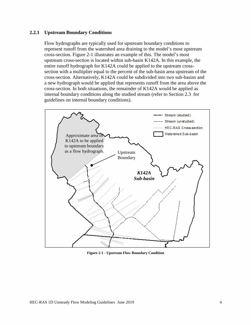
2.2.1 Upstream Boundary Conditions
Flow hydrographs are typically used for upstream boundary conditions to represent runoff from the watershed area draining to the model’s most upstream cross-section. Figure 2-1 illustrates an example of this. The model’s most upstream cross-section is located within sub-basin K142A. In this example, the entire runoff hydrograph for K142A could be applied to the upstream cross-section with a multiplier equal to the percent of the sub-basin area upstream of the cross-section. Alternatively, K142A could be subdivided into two sub-basins and a new hydrograph would be applied that represents runoff from the area above the cross-section. In both situations, the remainder of K142A would be applied as internal boundary conditions along the studied stream (refer to Section 2.3 for guidelines on internal boundary conditions).
Figure 2-1 - Upstream Flow Boundary Condition
K142A Sub-basin
Upstream Boundary
Approximate area of K142A to be applied to upstream boundary as a flow hydrograph.
HEC-RAS 1D Unsteady Flow Modeling Guidelines June 2019 5
2.2.2 Downstream Boundary Conditions
Downstream boundary conditions are required at all locations where flow leaves the model. This is typically a normal depth or rating curve at the most downstream cross-section of a reach, but it may also include storage areas (i.e., if a storage area is used to represent a permanent body of water such as a lake, bay, or ship channel). Downstream boundary locations should also be sufficiently downstream of the point of interest so as not to influence flows or water surface elevations at the study area. They should also be sufficiently far from hydraulic structures to prevent instabilities at the structure and/or downstream boundary. The following sections provide an overview and guidance on defining downstream boundary conditions.
2.2.2.1 Normal Depth
Normal depth should be used as the downstream boundary condition unless prior approval from HCFCD is obtained. In the majority of situations, the downstream water surface elevation and/or flow is unknown, and normal depth provides a reasonable estimate of these. Several situations where normal depth may not be adequate are discussed below. The normal depth method calculates an elevation based on Manning’s equation. To use this method, estimate the slope of the energy grade line that is generally the same as the channel bed slope. Because the normal depth calculation is sensitive to the estimate of the energy grade line, verify that the calculated normal depth is reasonable by comparing the water surface profile slope at the first few cross-sections at the downstream end of the stream with the channel bed slope. If the water surface profile slope is greater than the bed slope, reduce the starting normal depth energy slope. If the water surface profile is less than the bed slope, increase the starting normal depth energy slope. Normal depth should be used with caution in the situations discussed below due to potential instabilities and/or errors. In these situations, consider using other downstream boundary conditions such as rating curves and stage hydrographs instead of normal depth.
• Very mild slopes and/or where flow reverses (e.g., tidal zones and flat urban channels).
• Presence of backwater from a reach downstream of the model, if the timing of the backwater is coincident with the modeled reach (e.g., backwater from a main-stem reach that produces backwater up a minor tributary).
• Constant water surface (e.g., inline detention, bays, lakes, ship channels, etc.).
• Steep slopes that produce supercritical flow.
• Where the channel flows into large bodies of water with channel flowline well below static water level.
HEC-RAS 1D Unsteady Flow Modeling Guidelines June 2019 6
2.2.2.2 Rating Curves
A rating curve boundary condition applies a user-defined table to calculate the water surface elevation based on a given flow rate. Rating curves are typically used where channels flow into large bodies of water with a channel invert significantly below the ordinary water level in the water body (e.g., detention ponds, bays, lakes, ship channels, etc.). Normal depth is often invalid in these situations as the depth calculated can be well below that of the static pool elevation. Rating curves can be generated from physical measurements of the stream or from a steady-state model. Rating curves generated from physical measurements by HCFCD or the United States Geological Survey (USGS) are preferred over rating curves produced by a steady-state model. Rating curves with too few stage-flow points and abrupt changes can cause instabilities and/or errors; therefore, care should be taken when defining rating curves. Rating curves should be used with caution where looped rating curves are likely (i.e. very mild slopes and/or where flow reverses such as tidal zones) due to potential instabilities and/or errors.
2.2.2.3 Stage Hydrographs
A stage hydrograph boundary condition controls the stage at the downstream boundary location and is time dependent. It may only be used with the following downstream boundary types and requires approval by HCFCD.
• Tidal zones.
• Presence of backwater conditions from a receiving reach or permanent pool (e.g., bays and lakes) downstream of the model, if the timing of the backwater is coincident with the reach being modeled (e.g., a main-stem reach produces backwater up a minor tributary at the same time the tributary peak stage occurs).
• When modeling a historic storm event and the model’s downstream boundary is set at a stage gage with an observed historical record.

HEC-RAS 1D Unsteady Flow Modeling Guidelines June 2019 7
2.2.2.4 Flow Hydrographs
A flow hydrograph boundary condition defines the flow rate at the downstream boundary location. It may only be used to simulate historical events during model calibration and requires approval by HCFCD.
2.3 Internal Boundary Conditions
Internal boundary conditions are not required for a HEC-RAS unsteady flow model but must be included anywhere flow enters the model within the model boundaries. Therefore, in practice, most HEC-RAS unsteady flow models include internal boundary conditions. The most common internal boundary condition types are lateral inflow and uniform lateral inflow hydrographs representing runoff from watershed sub-basins generated from a HEC-HMS model. When using runoff hydrographs from a HEC-HMS model, confirm that runoff from sub-basins have not already been accounted for when a junction flow is applied. Care should also be taken to ensure that routings in HEC-HMS are not also being computed in HEC-RAS (i.e., do not ‘double count’ runoff or routings when using HEC-HMS as a source for HEC-RAS boundary conditions). Note that the locations and types of internal boundary conditions should be set up based on the 1% Annual Exceedance Probability (AEP) (i.e., 100-year) storm, not for each AEP, unless otherwise directed or approved by HCFCD. Also, boundary conditions cannot be set within one cross-section of internal boundaries (i.e., structures). The following sections provide an overview and guidelines for setting up internal boundary conditions.

HEC-RAS 1D Unsteady Flow Modeling Guidelines June 2019 8
2.3.1 Lateral Inflow Hydrographs
A lateral inflow hydrograph allows a single flow hydrograph to be applied to the model at a specific location (e.g., cross-section or storage area). Lateral inflow hydrographs should be used to apply point discharges to the modeled stream. For example, where tributaries discharge to the studied stream or where large storm-sewers discharge to the studied stream. Lateral inflows are to be applied to the first cross-section upstream of where the expected flow increases are anticipated to be observed. For example, in Figure 2-2, the grey area should be added as a lateral inflow hydrograph and assigned to the cross-section upstream of where the tributary stream joins the studied stream.
Figure 2-2 - Internal Lateral Inflow Boundary Condition (K142A)
K142A Sub-basin
Approximate area of K142A to be applied as
an internal, lateral inflow boundary
condition
Lateral inflow location
HEC-RAS 1D Unsteady Flow Modeling Guidelines June 2019 9
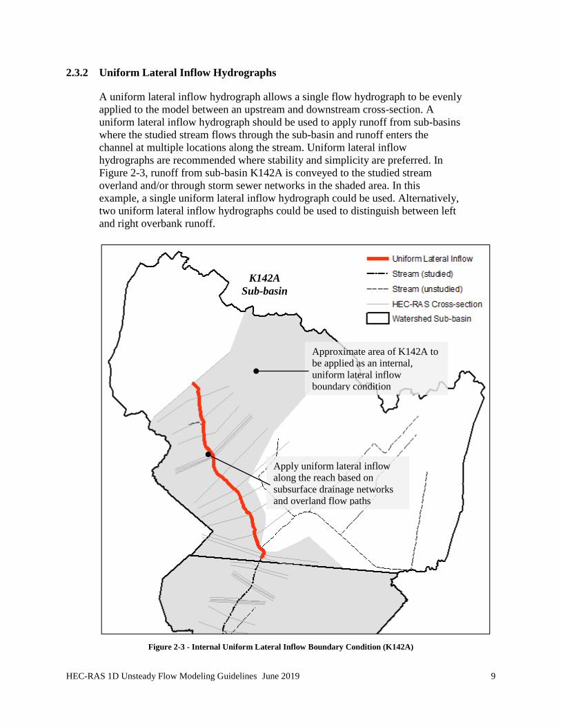
2.3.2 Uniform Lateral Inflow Hydrographs
A uniform lateral inflow hydrograph allows a single flow hydrograph to be evenly applied to the model between an upstream and downstream cross-section. A uniform lateral inflow hydrograph should be used to apply runoff from sub-basins where the studied stream flows through the sub-basin and runoff enters the channel at multiple locations along the stream. Uniform lateral inflow hydrographs are recommended where stability and simplicity are preferred. In Figure 2-3, runoff from sub-basin K142A is conveyed to the studied stream overland and/or through storm sewer networks in the shaded area. In this example, a single uniform lateral inflow hydrograph could be used. Alternatively, two uniform lateral inflow hydrographs could be used to distinguish between left and right overbank runoff.
Figure 2-3 - Internal Uniform Lateral Inflow Boundary Condition (K142A)
K142A Sub-basin
Apply uniform lateral inflow along the reach based on subsurface drainage networks and overland flow paths
Approximate area of K142A to be applied as an internal, uniform lateral inflow boundary condition
HEC-RAS 1D Unsteady Flow Modeling Guidelines June 2019 10
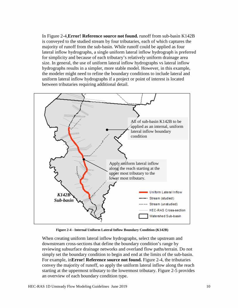
In Figure 2-4,Error! Reference source not found. runoff from sub-basin K142B is conveyed to the studied stream by four tributaries, each of which captures the majority of runoff from the sub-basin. While runoff could be applied as four lateral inflow hydrographs, a single uniform lateral inflow hydrograph is preferred for simplicity and because of each tributary’s relatively uniform drainage area size. In general, the use of uniform lateral inflow hydrographs vs lateral inflow hydrographs results in a simpler, more stable model. However, in this example, the modeler might need to refine the boundary conditions to include lateral and uniform lateral inflow hydrographs if a project or point of interest is located between tributaries requiring additional detail.
Figure 2-4 - Internal Uniform Lateral Inflow Boundary Condition (K142B)
When creating uniform lateral inflow hydrographs, select the upstream and downstream cross-sections that define the boundary condition’s range by reviewing subsurface drainage networks and overland flow paths/terrain. Do not simply set the boundary condition to begin and end at the limits of the sub-basin. For example, inError! Reference source not found. Figure 2-4, the tributaries convey the majority of runoff, so apply the uniform lateral inflow along the reach starting at the uppermost tributary to the lowermost tributary. Figure 2-5 provides an overview of each boundary condition type.
Apply uniform lateral inflow along the reach starting at the upper most tributary to the lower most tributary.
K142B Sub-basin
All of sub-basin K142B to be applied as an internal, uniform lateral inflow boundary condition

HEC-RAS 1D Unsteady Flow Modeling Guidelines June 2019 11
Figure 2-5 - Boundary Condition Overview (K142)
K142B Sub-basin
Lateral inflow at tributary discharge (upstream cross-section)
Upstream flow hydrograph boundary
Downstream stage or normal depth boundary
K142A Sub-basin
Uniform lateral inflow distributed along stream between tributaries
Uniform lateral inflow distributed along stream within sub-basin boundary

HEC-RAS 1D Unsteady Flow Modeling Guidelines June 2019 12
2.3.3 Internal Boundary Condition Rating Curves
As an internal boundary condition, rating curves most often are used to represent complex control structure (e.g., gates and weirs) that HEC-RAS cannot accurately represent or maintain a stable solution. While it is preferred to model control structures in HEC-RAS, rating curves may only be used for control structures where approved by HCFCD.
2.3.4 Internal Boundary Condition Stage Hydrographs
As an internal boundary condition, stage hydrographs are rarely used and require approval by HCFCD.
2.4 Minimum Flows
HEC-RAS unsteady flow requires every cross-section over the entire run simulation to be “wet” meaning a water surface must be present in every cross-section for every time step. A minimum flow rate can be specified to meet this requirement. The unsteady flow editor allows for each inflow hydrograph to have a minimum flow rate set. This is primarily used to maintain continuity when the model is initialized and reduce instabilities during low-flow periods. Engineering judgment and trial-and-error are required to determine the most suitable minimum flow rates and where minimum flows must be set. Adhere to the following guidelines when applying minimum flows:
• Use the lowest minimum flow value at the fewest locations necessary to produce a stable model initiation.
• Minimum flow rates throughout the model should be significantly less than the peak flow at all locations. Generally, minimum flows should approximate base flow conditions or be less than 5% of the 1% AEP peak flow.
• Confirm that storage volumes are not significantly reduced due to the constant minimum flow (e.g., the minimum flow should not result in a significant volume stored in cross-sections or offline storage areas).
2.5 Initial Conditions
Initial conditions are used to set initial values of flow and stage in order for HEC-RAS to compute the initial steady flow water surface profile. Initial flow values are required at upstream boundaries and the upstream cross-section of reaches below internal junctions.
HEC-RAS 1D Unsteady Flow Modeling Guidelines June 2019 13
2.5.1 Initial Flows
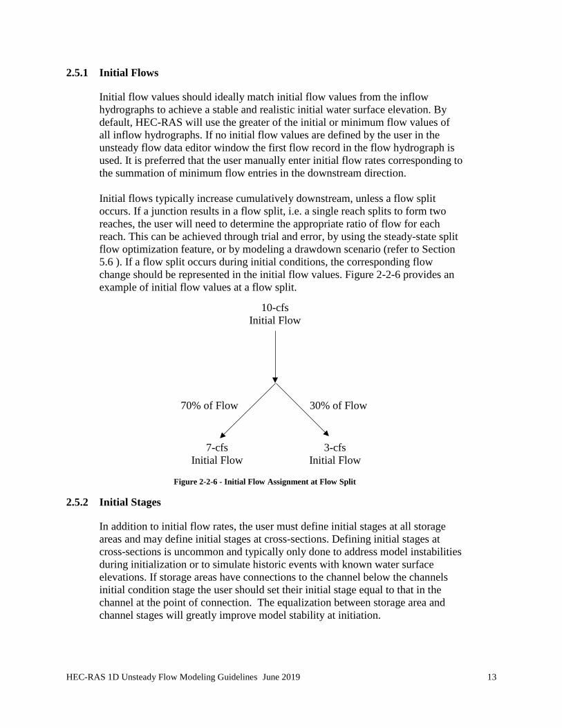
Initial flow values should ideally match initial flow values from the inflow hydrographs to achieve a stable and realistic initial water surface elevation. By default, HEC-RAS will use the greater of the initial or minimum flow values of all inflow hydrographs. If no initial flow values are defined by the user in the unsteady flow data editor window the first flow record in the flow hydrograph is used. It is preferred that the user manually enter initial flow rates corresponding to the summation of minimum flow entries in the downstream direction. Initial flows typically increase cumulatively downstream, unless a flow split occurs. If a junction results in a flow split, i.e. a single reach splits to form two reaches, the user will need to determine the appropriate ratio of flow for each reach. This can be achieved through trial and error, by using the steady-state split flow optimization feature, or by modeling a drawdown scenario (refer to Section 5.6 ). If a flow split occurs during initial conditions, the corresponding flow change should be represented in the initial flow values. Figure 2-2-6 provides an example of initial flow values at a flow split.
Figure 2-2-6 - Initial Flow Assignment at Flow Split
2.5.2 Initial Stages
In addition to initial flow rates, the user must define initial stages at all storage areas and may define initial stages at cross-sections. Defining initial stages at cross-sections is uncommon and typically only done to address model instabilities during initialization or to simulate historic events with known water surface elevations. If storage areas have connections to the channel below the channels initial condition stage the user should set their initial stage equal to that in the channel at the point of connection. The equalization between storage area and channel stages will greatly improve model stability at initiation.
10-cfs Initial Flow
7-cfs Initial Flow
3-cfs Initial Flow
30% of Flow 70% of Flow

HEC-RAS 1D Unsteady Flow Modeling Guidelines June 2019 14
SECTION 3 - COMPUTATION OPTIONS
In general, the HEC-RAS default Computation Options and Tolerances should be maintained. Where specified below, computation options may be changed from the default values to achieve model stability while maintaining computational accuracy. If other defaults are modified the modeler must document the changes and reasons these changes were necessary. 3.1 General Options
The following options may be changed from default values:
• Maximum number of iterations.
• Number of warm-up time steps.
• Time step during warm-up period.
The following options must be set to 3:
• Lateral and inline structure flow stability factors.
• Weir and gate flow submergence decay exponents.
3.2 Friction Slope Methods
Friction slope methods may be changed if approved by the HCFCD. In most cases, these methods should be set to default values.
3.3 Mixed Flow
The mixed flow option should not be used as a default method in models. It should only be selected if you actually have a mixed flow regime situation. It may be used in models that have periods of super-critical flow where standard approaches to improving stability were not successful. The Froude number factor and threshold values may be changed if approved by the HCFCD. In most cases, these methods should be set to default values.
3.4 Computation Intervals
The computation interval is one of the most important parameters entered into an unsteady flow model. The computation interval must be small enough to accurately describe the rise and fall of the hydrograph being routed. A general rule for selecting the computation interval is that the time step should be equal to or less than the time it takes water to travel from one cross-section to the next. For example, a model with a typical cross-section spacing of 500-feet and an estimated peak flood wave velocity of 5 ft/s would indicate a time step of less than 2-minutes. Often cross-sections near bridges are placed with much closer

HEC-RAS 1D Unsteady Flow Modeling Guidelines June 2019 15
spacing. Rapid rise and fall of water surface elevations often occur near bridges, culverts, and in-line weirs. With closer cross-section spacing and rapid changes in profiles, shorter computation intervals are often required. It is recommended that computation intervals of no greater than 1-minute be used for unsteady flow models to be submitted to HCFCD.
3.5 Advanced Time Step Control
Using the Advance Time Step Control option, the “Adjust Time Step Based on Courant” may be used to optimize the time step. Refer to the HEC-RAS 5.0.4 Supplemental UM_CPD-68d guidance manual for more information on this option. The Advance Time Step Control should be used only to assist in identifying a maximum fixed time step. Use of a fixed time step allows impact comparisons to be made between models ran with identical time steps. Alternative to a fixed time step, the user can use the “Adjust Time Step Based on Time Series of Divisors” under Advanced Time Step Control. This feature will allow for setting fixed time steps to be varied during certain portion of the simulation period. The selected times, time steps and divisor steps must be the same between models used for impact analysis. Use of this feature will allow for model comparisons based on identical time step computations while allowing for quicker model run times in some instances. Generally, a time step of 30 seconds or less fixed time step will often be required to produce a stable model. Use of the advance time step control will help identify an optimal time step.

HEC-RAS 1D Unsteady Flow Modeling Guidelines June 2019 16
SECTION 4 - GEOMETRY
4.1 Introduction
HEC-RAS unsteady flow requires additional attention be paid to geometry features as compared to steady flow. Poor quality data and/or data entered incorrectly are common causes of unstable and inaccurate unsteady flow models. The following sections provide an overview of geometric data guidelines and recommendations to be used when developing an unsteady flow model.
4.2 Cross-sections
The following are unsteady flow guidelines that are either specific to unsteady flow (i.e., not applicable to steady flow) or are in addition to those specified for cross-sections in HCFCD H&H Guidance Manual.
4.2.1 HTAB
Hydraulic Tables (HTAB) are used by HEC-RAS to compute rating curves at all cross-sections. This allows the HEC-RAS computational engine to perform calculations faster; however, those computations rely on the rating curves for a solution. A coarse and simplistic rating curve often results in inaccurate and unstable solutions.
The following minimum HTAB values should be used:
• Starting Elevation equal to the cross-section invert (e.g., flowline).
• Increment (i.e., spacing) of 0.1-ft.
• Number of Points sufficient to extend at least 2-ft above the 500-year WSE.
Following the above guidelines and updating values when cross-sections are modified will help create a robust and accurate unsteady flow model. Also note that HEC-RAS sets the HTAB values of interpolated cross-sections to the default. Even if HTAB values have already been set, they must be set for newly interpolated cross-sections.
4.2.2 Reach Lengths
Cross-section downstream reach lengths (i.e., cross-section spacing) should follow the guidance outlined in the HCFCD H&H Guidance Manual. In addition, cross-section spacing in an unsteady flow model should capture significant changes/transitions in overbank volume, since unsteady flow computations are based on volume. Figure 4-1 illustrates proper cross-section spacing to account for the entire overbank storage region and key transitions in the terrain. Note the location of cross-sections at the transition and shortly upstream and downstream

HEC-RAS 1D Unsteady Flow Modeling Guidelines June 2019 17
of the transition. In this case, interpolated cross-section station-elevation data should ideally rely on the actual terrain/bathymetry data.
Figure 4-1 - Overbank Volume
4.2.3 Obstructions
Obstructions may be used to represent areas that do not convey flow, should not be accounted for in storage volume routing, or are permanent water features. An example of using an obstruction in conjunction with an overbank storage area is shown in Figure 4-2. Refer to Section 4.6 for details on using storage areas.
Figure 4-2 - Example of Obstructed Area Modeled as Storage Area
Area blocked and modeled using storage area
Area blocked and modeled using storage area
Incorporates key transitions in overbank terrain
Cross-section with blocked areas
HEC-RAS 1D Unsteady Flow Modeling Guidelines June 2019 18
4.2.4 Ineffective Flow
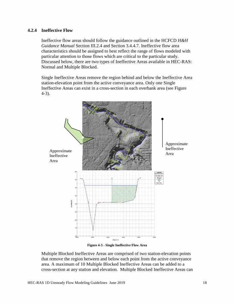
Ineffective flow areas should follow the guidance outlined in the HCFCD H&H Guidance Manual Section III.2.4 and Section 3.4.4.7. Ineffective flow area characteristics should be assigned to best reflect the range of flows modeled with particular attention to those flows which are critical to the particular study. Discussed below, there are two types of Ineffective Areas available in HEC-RAS: Normal and Multiple Blocked. Single Ineffective Areas remove the region behind and below the Ineffective Area station-elevation point from the active conveyance area. Only one Single Ineffective Areas can exist in a cross-section in each overbank area (see Figure 4-3).
Figure 4-3 - Single Ineffective Flow Area
Multiple Blocked Ineffective Areas are comprised of two station-elevation points that remove the region between and below each point from the active conveyance area. A maximum of 10 Multiple Blocked Ineffective Areas can be added to a cross-section at any station and elevation. Multiple Blocked Ineffective Areas can
Approximate Ineffective Area
Approximate Ineffective Area

HEC-RAS 1D Unsteady Flow Modeling Guidelines June 2019 19
be used for complex areas in an attempt to better reflect actual conveyance conditions (see Figure 4-4) and/or improve model stability by creating gradual changes in effective flow area (see Figure 4-5).
Figure 4-4 - Multiple Blocked Ineffective Areas - To Reflect Geometry
Ineffective Areas can also be set to permanent or non-permanent. Permanent Ineffective Areas continue to remove the area from active conveyance after the water surface elevation exceeds the Ineffective Area elevation. Non-permanent Ineffective Areas are temporarily turned off if the water surface elevation exceeds the Ineffective Areas elevation. Non-permanent Ineffective Areas generally cause instabilities near the Ineffective Area elevation due to a significant change in conveyance area that can occur over a single time step.
Figure 4-5 - Example of Multiple Blocked Ineffective Areas - For Stability
Stepped to improve stability

HEC-RAS 1D Unsteady Flow Modeling Guidelines June 2019 20
When evaluating whether to use permanent versus non-permanent ineffective areas, their elevation, and their station, the modeler must play close attention to flow continuity. Reviewing flow in the overbanks both approaching and leaving a structure along with computed weir flow over a structure should be considered when setting ineffective flow area conditions. Given the limitations of ineffective areas (particular upstream and downstream of bridges and culverts), the modeler should give preference to achieving a simple, stable model versus a theoretically perfect representation of the ineffective flow condition. Ultimately it is the modeler’s responsibility to define ineffective flow characteristics based on the purpose and required level of accuracy of the unsteady flow model. If the modeler believes the area of interest is too complex to represent conveyance accurately using 1D cross-sections and ineffective areas, consider converting the area to a combined 1D/2D model.
4.2.5 Contraction and Expansion Coefficients
Contraction and expansion coefficients are not, by default used in unsteady flow modeling. However, they may be considered where abrupt changes occur, model results are not matching observed data, and the modeler believes this is due to the Momentum equation not accurately representing losses at that location. In this scenario, the modeler should demonstrate their rationale and obtain approval by HCFCD. Typical applicability will be in locations introducing major changes in the energy slope such as bridges. To employ the use of contraction/expansion coefficients in unsteady flow modeling, they are defined within the geometry editor, under tables, Contraction/Expansion Coefficients (Unsteady Flow).
4.2.6 Pilot Channels
Pilot channels are used to assist in initializing and maintaining a stable low-flow condition in an unsteady flow model. They are helpful when initial flow rates produce shallow depths (i.e., less than 1-ft) and/or the slope increases downstream (see Figure 4-6). In these conditions, small changes in flow can have significant changes in depth percentage wise causing instabilities and the model fails to converge on a solution due to large oscillations.
Pilot channels offer a simple and elegant solution to the common problem by providing depth to the cross-section at low flows. The user defines the slot width, initial depth, and slope, resulting in either a constant or variable sized Pilot Channel throughout the reach. The Pilot Channel aides the model in producing a solution in which the actual channel is dry while the pilot channel maintains a positive depth (see Figure 4-6). The additional depth of the Pilot Channel produces minimal additional flow area (assuming a reasonable slot depth and width is used) and is ignored during high flows (see Figure 4-7). The pilot channel further improves low flow stability by smoothing out channel flowline irregularities.

HEC-RAS 1D Unsteady Flow Modeling Guidelines June 2019 21
Figure 4-6 - Example of a Pilot Channel (Profile View)
The following criteria should be considered when using Pilot Channels:
• Recommended width of less than 2-ft.
• Recommended minimizing depth while providing a positive downstream slope. A variable slope Pilot Channel is usually needed for long channels with a variable sloped flowline.
• Recommended Manning’s n value equal to or greater than channel Manning’s n value.
Figure 4-7 - Example of a Pilot Channel (Cross-section View)
Pilot channel allows a solution below the channel invert
HEC-RAS 1D Unsteady Flow Modeling Guidelines June 2019 22
4.2.7 Lidded Cross-sections
Lids may be added to cross-sections to represent long tunnels where a culvert feature is not practical or where flow changes are required within the culvert reach. HEC-RAS will treat the cross-section as an open channel cross-section while removing the lid’s area and including the lid’s wetted perimeter in computations. Lidded cross-sections should also be used if the volume within the conduit needs to be considered. Unsteady HEC-RAS does not compute volume within conduits as part of the calculations. Other uses for lidded cross-sections could include modeling of siphons or broken back culverts.
4.2.7.1 Priessman Slot
The user may add a Priessmann Slot to lidded cross-sections to model the lidded cross-sections as a pressurized pipe. Note that this option is only used in Unsteady Flow and is therefore not used in a Steady Flow analysis.
4.3 Bridge and Culvert Structures
Bridges and culverts should follow the guidance outlined in the H&H Guidance Manual. Unsteady flow requires additional parameters that must be defined, as discussed in the following sections.
4.3.1 Options
Unless noted below, all parameters found in the Options menu under the Bridge/Culvert editor should remain at default values unless approved by the HCFCD.
Internal cross-sections may be modified without prior approval by the HCFCD. Internal cross-sections are automatically created by HEC-RAS based on the bounding cross-sections and the bridge structure; therefore, they may not accurately represent the bridge opening. For example, they may be modified to match the bridge opening if the bounding cross-section flowlines and/or banks encroach on the bridge opening. This scenario often results in bridge opening calculations not replicating actual conditions. Manning’s n values may also be adjusted to reflect the bridge opening material (e.g., concrete slope paving) if different than the channel (e.g., earthen channel). Any modifications to internal cross-sections must be noted in the bridge description.

HEC-RAS 1D Unsteady Flow Modeling Guidelines June 2019 23
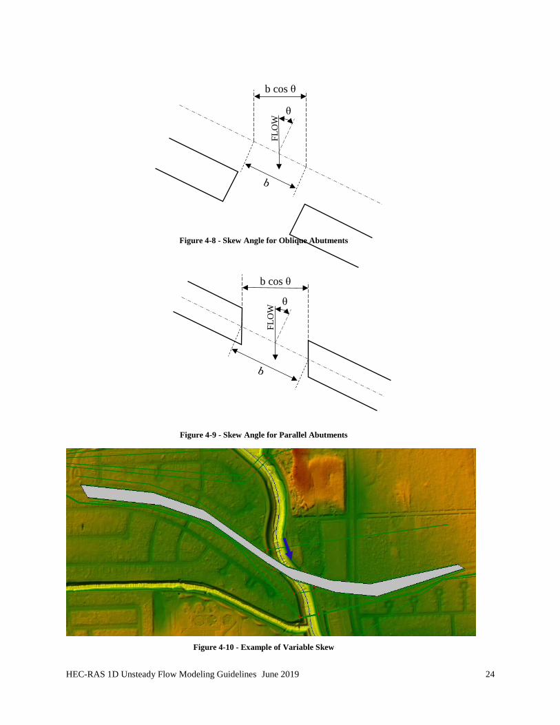
4.3.1.1 Skew
Skew angles may be applied to bridges, piers, and/or bounding cross-sections as necessary. Figure 4-8 and Figure 4-9 illustrate how to calculate bridge skew angles for oblique and parallel abutments (Bradley, J. (1960). Hydraulics of Bridge Waterways (Hydraulic Design Series No. 1). Division of Hydraulic Research, Bureau of Public Roads, U.S. Department of Commerce, Washington D.C.). A skew angle is not required for angles of 20 degrees or less. Application of a skew should be avoided when possible by improved cross-section alignment.
Often, a skew angle is incorrectly applied to an entire cross-section where the channel is skewed but overbanks are not (see Figure 4-10, where the right overbank and channel are skewed approximately 45-degrees while the left overbank is not skewed). Applying a 45-degree skew to the entire cross-section would underestimate overbank volume and cause instabilities. The modeler must determine whether the bridge and/or cross-sections are skewed in the left overbank, channel, and right overbank. If one of these sections is not skewed, the modeler must create “composite” station-elevation data since HEC-RAS only allows for a single skew angle to be applied to the entire bridge and cross-section.
HEC-RAS 1D Unsteady Flow Modeling Guidelines June 2019 24
Figure 4-8 - Skew Angle for Oblique Abutments
Figure 4-9 - Skew Angle for Parallel Abutments
Figure 4-10 - Example of Variable Skew
θ
b cos θ
FL
OW
θ
b cos θ F
LO
W

HEC-RAS 1D Unsteady Flow Modeling Guidelines June 2019 25
4.3.2 HTAB
Similar to cross-sections, bridges require HTAB values to create a family of rating curves when pre-processing the geometry. HEC-RAS requires that the user enters values for the following:
• Number of points on free flow curve (valid range of 10 to 100).
• Number of submerged curves (valid range of 10 to 60).
• Number of points on each submerged curve (valid range of 10-50).
• Headwater maximum elevation.
It is recommended to accept the default of settings for each of the above curves and a headwater maximum elevation greater than the anticipated 500-year WSE. However, the optimal number of points and headwater maximum elevation will depend on the flood events being modeled and the characteristics of the model. While more points and a lower headwater maximum elevation generally results in a more stable model, this is not always the case. For example, fewer points will simplify the rating curves and result in a ‘smoothing’ of the hydraulic structure’s performance. This may result in a more stable model, but may also reduce the model’s accuracy and therefore potentially reduce the model’s stability. Another example that should be watched for is whether a single point on the curves falls at the same elevation as the bridge deck. This could result in a sudden change in flow for a minor change in elevation, which may be realistic, but may also result in an unstable model. Reducing or adding points or changing the headwater maximum elevation could all improve or worsen the situation. The best approach is often trial and error.
As such, the recommendation above is intended to provide a fairly stable and accurate solution for typical models; however, the modeler should review and revise these values as needed to achieve a stable and accurate solution for their situation.
The following values are optional within HEC-RAS but required by the HCFCD, as they can significantly improve model stability and accuracy.
• Tailwater maximum elevation.
• Maximum flow.
The tailwater maximum elevation and maximum flow values should be set based on the maximum storm event being modeled. In most cases, this will be the 500-year event. Note that the elevation and flow should be set slightly above the 500-year event, not exactly equal to the 500-year event. Each of these values will further refine the family of rating curves, resulting in high-resolution curves that generally will result in a more stable and accurate model. However, as discussed

HEC-RAS 1D Unsteady Flow Modeling Guidelines June 2019 26
above, the modeler should review and revise these values as needed to achieve a stable and accurate solution for their situation. Note that the modeler may not manually modify the curves.
4.3.3 Bridge Modeling Approach
The Energy Method (Standard Step) for low and high flow methods should typically be used. Momentum (for low flow) and Pressure and/or Weir (for high flow) methods may be used where necessary to improve model stability and/or accuracy but should be noted in the bridge description. For example, Momentum for low flow may be more applicable where the majority of losses are due to the bridge piers. Associated coefficients for each method should follow the HCFCD H&H Guidance Manual.
4.4 Inline Weirs
Inline weirs are used to represent structures in the channel that impede flow. These structures may include culverts, gates, and/or openings. Parameters for weir and culvert components should follow guidelines discussed in Section 0. By default, HEC-RAS computes flow through/over the weir based on culvert and/or weir flow; however, the Outlet Rating Curve option may be used if a rating curve exists. Use of the Outlet Rating Curves are not typical and requires approval by the HCFCD. Inline weirs may also be used to improve model stability where sudden changes in channel flowline can cause the model to quickly transition from subcritical to supercritical flow and where a pilot channel and/or mixed flow does not resolve the instability. As shown in Figure 4-11, an inline weir can be added just upstream of the transition, forcing the model to compute the transition using the weir equation versus the Momentum Equation. A note should be added to the weir description stating that it is a fictitious structure added for stability.
Figure 4-11 - Inline Weir Added for Stability
HEC-RAS 1D Unsteady Flow Modeling Guidelines June 2019 27
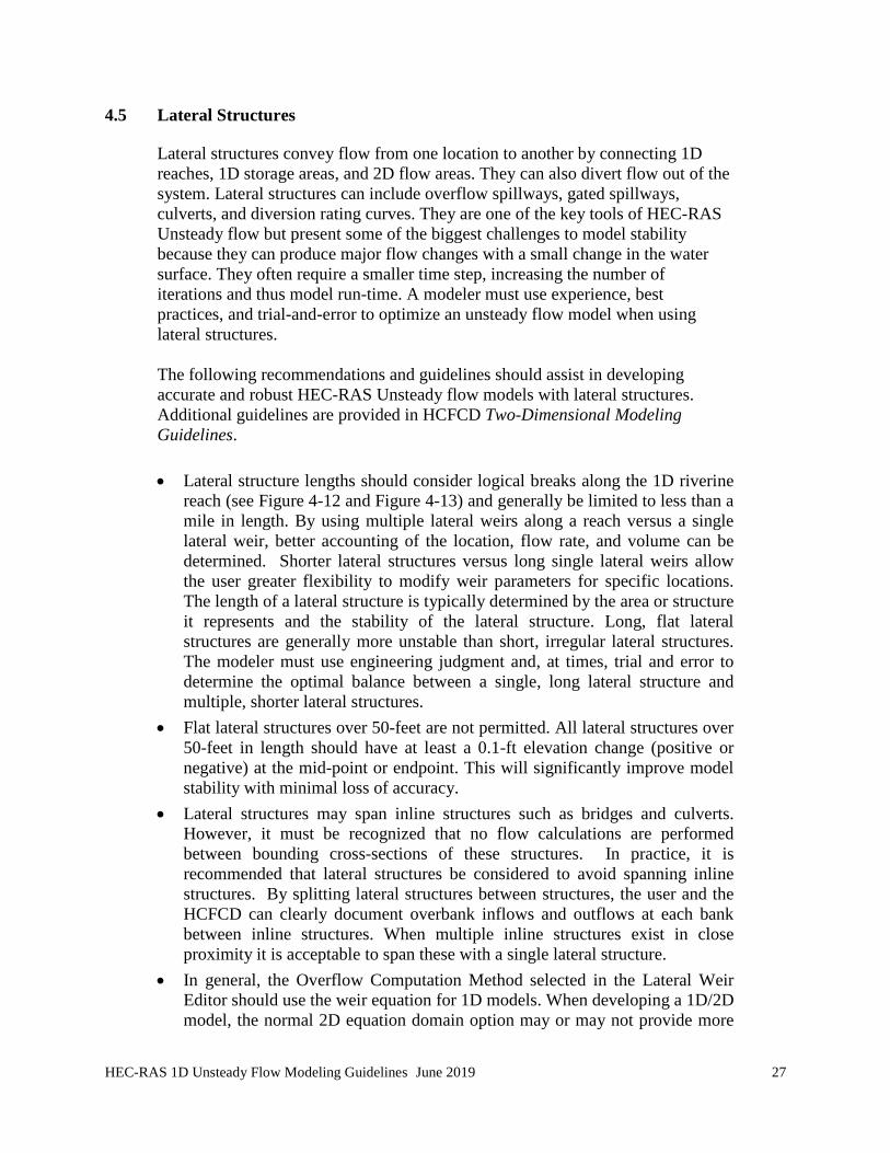
4.5 Lateral Structures
Lateral structures convey flow from one location to another by connecting 1D reaches, 1D storage areas, and 2D flow areas. They can also divert flow out of the system. Lateral structures can include overflow spillways, gated spillways, culverts, and diversion rating curves. They are one of the key tools of HEC-RAS Unsteady flow but present some of the biggest challenges to model stability because they can produce major flow changes with a small change in the water surface. They often require a smaller time step, increasing the number of iterations and thus model run-time. A modeler must use experience, best practices, and trial-and-error to optimize an unsteady flow model when using lateral structures. The following recommendations and guidelines should assist in developing accurate and robust HEC-RAS Unsteady flow models with lateral structures. Additional guidelines are provided in HCFCD Two-Dimensional Modeling Guidelines.
• Lateral structure lengths should consider logical breaks along the 1D riverine reach (see Figure 4-12 and Figure 4-13) and generally be limited to less than a mile in length. By using multiple lateral weirs along a reach versus a single lateral weir, better accounting of the location, flow rate, and volume can be determined. Shorter lateral structures versus long single lateral weirs allow the user greater flexibility to modify weir parameters for specific locations. The length of a lateral structure is typically determined by the area or structure it represents and the stability of the lateral structure. Long, flat lateral structures are generally more unstable than short, irregular lateral structures. The modeler must use engineering judgment and, at times, trial and error to determine the optimal balance between a single, long lateral structure and multiple, shorter lateral structures.
• Flat lateral structures over 50-feet are not permitted. All lateral structures over 50-feet in length should have at least a 0.1-ft elevation change (positive or negative) at the mid-point or endpoint. This will significantly improve model stability with minimal loss of accuracy.
• Lateral structures may span inline structures such as bridges and culverts. However, it must be recognized that no flow calculations are performed between bounding cross-sections of these structures. In practice, it is recommended that lateral structures be considered to avoid spanning inline structures. By splitting lateral structures between structures, the user and the HCFCD can clearly document overbank inflows and outflows at each bank between inline structures. When multiple inline structures exist in close proximity it is acceptable to span these with a single lateral structure.
• In general, the Overflow Computation Method selected in the Lateral Weir Editor should use the weir equation for 1D models. When developing a 1D/2D model, the normal 2D equation domain option may or may not provide more
HEC-RAS 1D Unsteady Flow Modeling Guidelines June 2019 28
stable and accurate results. Current evaluations have shown with the low velocities often encountered within Harris County that the weir equation with a low weir coefficient often provides a more stable model with results negligibly different than that of the 2D equation. When using the Weir Equation, refer to Table 4-1 and the HCFCD Two-Dimensional Modeling Guidelines document for recommended coefficient values.
Figure 4-12 - Example of Lateral Structures at Bridges
Break at major bridge
Break at major bridge

HEC-RAS 1D Unsteady Flow Modeling Guidelines June 2019 29
Figure 4-13 - Example of Lateral Structures at Basins
• In general, lateral structure weir coefficients should be lower than typical inline weirs. Whenever possible, weir coefficients should be calibrated to produce reasonable results.
Table 4-1 - Lateral Structure Weir Coefficients
Item Being Modeled with Lateral Structure
Description Range of Weir Coefficients
Levee/roadway: 3 feet or higher above natural ground
Broad crested weir shape, flow over levee/road acts like weir flow
1.5 to 2.6 (2.0 default)
Levee/roadway: 1 to 3 feet above natural ground
Broad crested weir shape, flow over levee/road acts like weir flow, but
becomes submerged easily
1.0 to 2.0
Natural high ground barrier: 1 to 3 feet high
Does not really act like a weir, but water must flow over high ground to get into
2D flow area
0.5 to 1.0
Non elevated overbank terrain, lateral structure not
elevated above ground
Overland flow escaping the main channel 0.2 to 0.5
Tributary Lateral structure represents the cross-section of a tributary with a depth ≥ 6-ft
at the confluence
2.0
Break at Proposed Basin
Break to limit total length
Captures spillway and berm
Break to allow separate parameters and accounting of tributary flow
HEC-RAS 1D Unsteady Flow Modeling Guidelines June 2019 30
• Use of Linear Routing as a lateral structure type is not common and requires approval by the HCFCD.
• Lateral structures that represent terrain/ground features should be created using GIS coordinates (e.g., use the HEC-RAS Geometry measure tool to draw the lateral structure and copy-paste the cutline coordinates). This will allow the user and the HCFCD to visually match the lateral structure with the overflow location.
• Compute weir flow using the water surface. The majority of lateral structures in Harris County will be located adjacent to the main channel, where weir flow is best computed using the water surface.
• The weir width is used for visualization purposes and does not affect computations.
• Set the weir crest shape to Broad Crested by default. Use of other shapes where appropriate requires approval by the HCFCD and documentation in the lateral structure description.
• Use of a Diversion Rating Curve requires approval by the HCFCD. It should only be used where a known, fixed diversion occurs or where a complex control structure cannot be modeled accurately in HEC-RAS and a known rating curve is available.

HEC-RAS 1D Unsteady Flow Modeling Guidelines June 2019 31
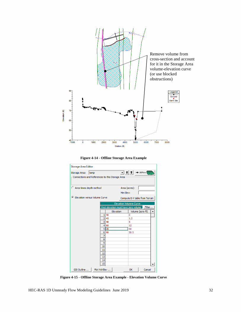
4.6 Storage Areas
Storage areas are generally used to model inline or offline ponding areas (e.g., detention basins) because their computations are more stable and faster than using cross-sections. Storage areas rely on the Continuity equation (not Momentum) and a stage-storage rating curve. They are connected to cross-sections and 2D flow areas using lateral structures and other storage areas using storage area connectors. Storage area boundaries should be delineated to match the outline of the feature being modeled. For example, if the storage area models a detention basin to top of the berm, the storage area boundary should match the berm outline. Storage areas should include elevation vs. storage curves based on the model terrain, design plans, or as-builts. The area times depth method may be used for simple analyses. Offline storage areas may have cross-sections trimmed to the edge of the bank or extended over the storage area. In most cases, the modeler will likely extend the cross-sections over the storage area to allow for conveyance to be computed across the top of the basin during high flow events allowing for a simpler, straightforward comparison between existing and proposed conditions (assuming the storage area includes the proposed basin volume). Figure 4-14 provides an example of an offline storage area with cross-sections extended over the proposed basin. It is critical that the modeler properly assigns the storage area volume to the storage area vs. the cross-sections. In the example, the storage area is used to represent volume below the top of the bank and the cross-section used to represent volume above top of bank. The storage area volume-elevation curve includes volume from the flowline to top of bank. The storage curve should include a stage above top of bank with a very slight increase in volume (see Figure 4-15). This will allow for out-of-bank flood stages to match between the basin and the 1D cross-section. The cross-section station-elevation data below top of bank do not include the storage area grading. This prevents double accounting of volume and allows for effective flow above top of bank to be captured in the cross-sections. In this situation, the manning’s n value of the cross-section within the basin should be set between 0.2 to 0.3. Alternatively, the cross-section could have included the storage area terrain profile and used a blocked obstruction to remove the storage area volume.
HEC-RAS 1D Unsteady Flow Modeling Guidelines June 2019 32
Figure 4-14 - Offline Storage Area Example
Figure 4-15 - Offline Storage Area Example - Elevation Volume Curve
Remove volume from cross-section and account for it in the Storage Area volume-elevation curve (or use blocked obstructions)

HEC-RAS 1D Unsteady Flow Modeling Guidelines June 2019 33
4.6.1 Storage Area Connectors
Storage area connectors are used to connect two storage areas. A single storage area may be connected to multiple other storage areas using multiple connectors. Storage area connector structure types include weir, weir and culvert, and linear routing. A weir or weir and culvert structure type is typically used and should follow the guidelines outlined in the previous sections. Use of Linear Routing requires approval by the HCFCD. Storage area connectors should be drawn from left to right looking downstream (i.e., the direction of flow) so that the headwater and tailwater are indicated correctly.
4.7 Junctions
Junction nodes are used to join and/or split three or more reaches and balance water surface elevations at each cross-section nearest the junction. HEC-RAS uses the distance to the upstream cross-section in the Junction Editor to balance water surface elevations across junctions (i.e., HEC-RAS does not use cross-section downstream reach lengths). For unsteady flow models, water surface elevations at junctions should, by default, be computed using the Energy Balance method. This ensures that each cross-section nearest the junction has an individual water surface elevation computed. However, if the cross-sections are closely spaced (e.g., 50-ft), the channel does not have a steep slope, and the water surface elevations will likely be close in elevation, the Force Equal WS Elevations option may be used. This will provide a more stable and faster solution in these situations. Alternatively, the use of storage areas and lateral weirs may be used as junctions for combining and splitting stream reaches (see Figure 4-16 and Figure 4-17). A 1D Storage Area feature “replaces” the junction node and is drawn at the downstream end of the tributary reach. The tributary is connected to the Storage Area and lateral structures added on the tributary to convey overland flow from upstream of the Storage Area to the main reach (see Figure 4-16 and Figure 4-17). A lateral structure is then added to the main reach with the tailwater set to the Storage Area. Weir coefficients should be set to reflect the likely head loss across the junction. A value of 2.0 appears to produce the most stable and reasonable results in Harris County where backwater often controls the water surface in the tributary; however, it is up to the modeler to determine a reasonable coefficient based on the specific area. A 2D Flow Area may be considered instead of a Storage Area; however, the Storage Area will generally produce a more stable solution and thus may be more practical. This approach provides a stable and robust solution while allowing the main river to be built using a single reach. The approach has been shown to provide results equivalent to the Energy Balance method for areas in Harris County where
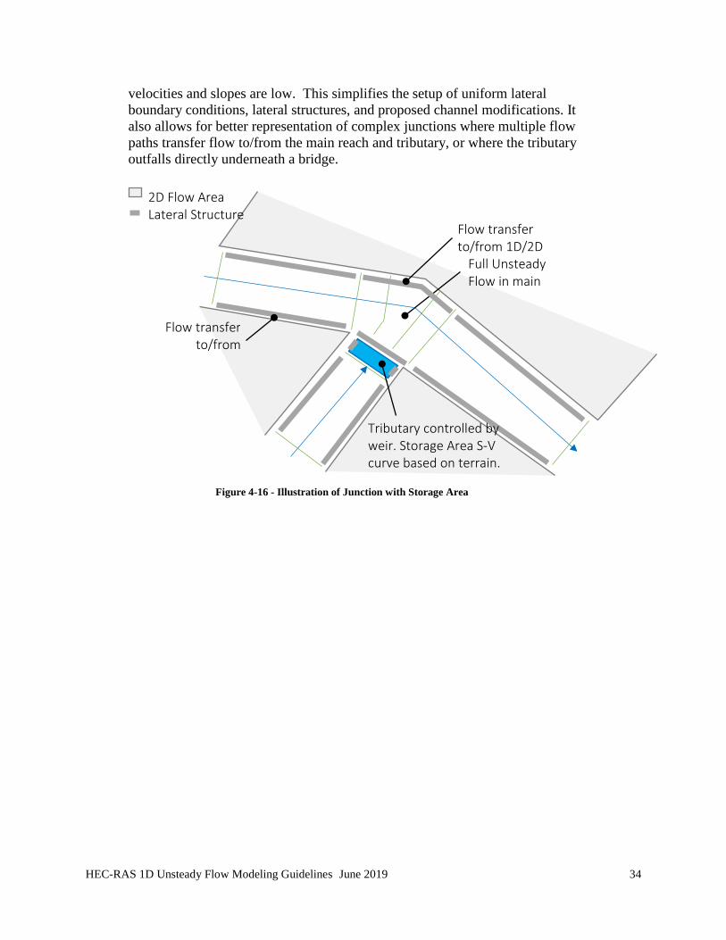
HEC-RAS 1D Unsteady Flow Modeling Guidelines June 2019 34
velocities and slopes are low. This simplifies the setup of uniform lateral boundary conditions, lateral structures, and proposed channel modifications. It also allows for better representation of complex junctions where multiple flow paths transfer flow to/from the main reach and tributary, or where the tributary outfalls directly underneath a bridge.
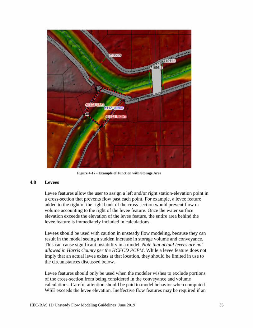
Figure 4-16 - Illustration of Junction with Storage Area
2D Flow Area Lateral Structure
Full Unsteady Flow in main
Flow transfer to/from
Flow transfer to/from 1D/2D
Tributary controlled by weir. Storage Area S-V curve based on terrain.
HEC-RAS 1D Unsteady Flow Modeling Guidelines June 2019 35
Figure 4-17 - Example of Junction with Storage Area
4.8 Levees
Levee features allow the user to assign a left and/or right station-elevation point in a cross-section that prevents flow past each point. For example, a levee feature added to the right of the right bank of the cross-section would prevent flow or volume accounting to the right of the levee feature. Once the water surface elevation exceeds the elevation of the levee feature, the entire area behind the levee feature is immediately included in calculations. Levees should be used with caution in unsteady flow modeling, because they can result in the model seeing a sudden increase in storage volume and conveyance. This can cause significant instability in a model. Note that actual levees are not allowed in Harris County per the HCFCD PCPM. While a levee feature does not imply that an actual levee exists at that location, they should be limited in use to the circumstances discussed below. Levee features should only be used when the modeler wishes to exclude portions of the cross-section from being considered in the conveyance and volume calculations. Careful attention should be paid to model behavior when computed WSE exceeds the levee elevation. Ineffective flow features may be required if an

HEC-RAS 1D Unsteady Flow Modeling Guidelines June 2019 36
area receiving volume behind a levee feature does not fully convey flow. Additionally, if an area receives flow and has significant volume capacity, but is likely to have a lower WSEL than the channel side of the levee feature, alternative modeling techniques should be employed. For example, modeling overbank areas that fill separately or have a WSEL not directly connected to the channel WSEL may require the use of a lateral structure connected to storage areas, 2D flow areas, and/or a separate reach. This will provide a more accurate result and allow for greater flexibility and stability when modeling.
Figure 4-18 - Example of Levee and Ineffective Flow Features
Hydraulically connected but ineffective
Hydraulically connected but ineffective
Consider modeling area as a 2D Flow Area
Consider modeling area as a 2D Flow Area
Hydraulically connected but ineffective Hydraulically connected
but ineffective

HEC-RAS 1D Unsteady Flow Modeling Guidelines June 2019 37
SECTION 5 - MODEL DEBUGGING
The following section summarizes common “debugging” techniques and best practices. While the ultimate goal is a robust, reasonably accurate model, getting there is often challenging and requires experience and training. The following sections provide basic techniques based on experience developing complex unsteady flow models for urban areas like Harris County. 5.1 Data Quality
Ensuring that the data used to generate the model is high quality and correct will resolve a lot of issues and generally increase both robustness and accuracy. Given the high quality of LiDAR, it should be straightforward to incorporate high-quality terrain data in overbanks. Structure data should be surveyed with visual inspections (photos) documenting size and number of openings. Overbank elevations should be blended with channel bathymetry based on survey and/or LiDAR where applicable.
5.2 Cross-Sections
Properly laying out and spacing cross-sections based on flow paths and areas, time step, slope, and velocity is critical. Cross-section spacing and layout should follow the guidance outlined in Section 4.2 and the HCFCD H&H Guidance Manual. The following is additional guidance to help identify issues and/or improve stability.
5.2.1 Common Sources of Instability
The following are common sources of instability and recommended techniques for resolving instabilities related to cross-sections:
• Rapid changes in flow area due to sudden changes in cross-section area between cross-sections
o Add cross-sections, preferably with station-elevation data based on actual terrain and bathymetry data. If data is unavailable, simply interpolate to provide a transition in flow area between cross-sections. Balance cross-section spacing with velocity and time step as discussed in Section 4.2.2 .
o Add ineffective flow and/or blocked areas where realistic and within reason to reduce changes in flow area.
• Rapid changes in flow area in and out of culvert/bridge structures.
o Culverts may have silt deposits or erosion occurring near the entrance and exits of the structures. This may result in the model seeing large grade changes as the flow enters or exits the structures. Modifying the internal cross-sections to match the structure low flow opening or in the case of
HEC-RAS 1D Unsteady Flow Modeling Guidelines June 2019 38
culverts including the sediment as a blocked obstruction within the culvert.
• Super- and sub-critical flows due to high velocities, rapid increases in slope, and/or drops in the channel flowline.
o Run using the Mixed Flow Option turned on if mixed flow regime conditions are present (see Calculation Options and Tolerances within the Unsteady Analysis window and the 1D Mixed Flow Options tab; Check “Mixed Flow Regime”).
o Modify Manning’s n values by a minimal, reasonable amount (e.g., from 0.013 to 0.015) to see if this improves stability. Generally, lower Manning’s n values will create supercritical flow issues during start-up. By increasing the Manning’s n value in areas where the model first computes critical flow it may force a subcritical solution and allow the model to continue to run.
o Add an inline weir structure and/or pilot channel as discussed in Section 4.4 and Section 4.2.6 .
• Overly complex Manning’s n values. Manning’s n-values should follow the guidance specified in the HCFCD H&H Guidance Manual. However, when following best practices and guidelines, it is tempting to represent every change in Manning’s n value. Doing so can have unintentional negative impacts on model accuracy and/or stability. Simplifying Manning’s n-values can often avoid this issue and improve stability without significantly affecting accuracy. Specifically, care should be taken in the following situations:
o Horizontal n values with small spacing combined with Multiple Ineffective areas, particularly when used within the left and right banks. This can create sudden changes in the conveyance area and n-values for small changes in flow and/or WSEL.
o High n-values on channel side slopes and/or benched areas within the left and right bank stations. Instability often occurs due to a large increase in the weighted channel n-value from a small increase in WSEL.
o Low n-values (e.g., 0.013 for concrete channels) for an entire cross-section within the left and right bank stations when combined with high velocities (e.g., > 7 ft/sec). While this scenario may run fine in some situations, it can also cause difficult to diagnose instabilities depending on the channel and bank slopes (i.e., areas of rapid change in slope and/or steep or vertical channel banks).
o Review of the channel n-value from the tabular report should be performed to identify cross-sections that have abrupt changes in n-values when compared to bounding cross-sections.
HEC-RAS 1D Unsteady Flow Modeling Guidelines June 2019 39
5.2.2 Common Data Issues
The following are common cross-section data issues that modelers should be aware of:
• Differences between the total reach length and the actual length of the reach centerline. A simple check can be performed by comparing the Reach Invert Line Length (found in the Geometry Window under GIS Tools, then click Compute Line Length) to the sum of all Channel Downstream Reach Lengths (calculated in Excel). If the model was developed from HEC-GeoRAS with the channel flow path layer copied from the river centerline layer, these should match exactly. More than likely, there will be a difference, particularly for highly sinuous systems with large 100-yr floodplains, where the model has been calibrated for the 100-yr event. Nevertheless, this comparison is often useful and can help identify double counting or loss of reach lengths at specific cross-sections, which often account for major instabilities (not to mention loss of accuracy).
• Differences in the cross-section cut line length and the length based on the station-elevation data. Differences can be identified by turning on the Ratio of Cut Line Length to XS Length (found in the Geometry Window under View Options and Cross-Section Properties). Ratios should equal 1.0 but realistically could span +/- 5% (i.e., 0.95 to 1.05). Ratios greater than 1.0 indicate that station-elevation data is missing or the cut-line is too long. Ratios less than 1.0 indicate the cut-line is too short or there is extra station-elevation data.
5.3 Start-Up and Low Flows
A few simple techniques can resolve most start-up/initialization and low flow issues. With experience and the following techniques, initializing a model should be relatively straightforward.
• Ensure that initial flow rates match the initial flow rates found in the internal boundary conditions (refer to Section 2.5 ).
• Add a minimum flow to the most upstream inflow hydrograph at a rate sufficient to create a low-flow condition (refer to Section 2.4 ).
• Add pilot channels and/or fictitious inline weirs where the enters supercritical flow through sharp drops (refer to Section 4.2.6 ).
• Use warm-up time steps to help generate a stable numerical solution prior to the initial time step.
• Storage areas connected to reaches should have an initial stage set that closely matches the initial WSELs in the receiving channel. (refer to Section 2.5.2 ).

HEC-RAS 1D Unsteady Flow Modeling Guidelines June 2019 40
5.4 High Flows
Debugging high-flows (i.e., bank-full and out-of-bank flows) presents several common challenges, including:
• Overtopping of inline structures (e.g., bridges, weirs, and culverts).
• Overtopping of banks which can activate lateral structures, or if cross-sections extend into overbanks, can activate levees, blocked obstructions, and ineffective flow areas. Overbank flow can also cause instabilities due to simplification of overbank storage volumes and flow paths when using cross-sections vs. 2D Flow Areas.
• Higher velocities and super-critical transitions.
• Reverse flow due to backwater from structures and/or downstream tailwater.
• Review flow continuity across cross-section and structures to avoid un-realistic changes in the flow computed between cross-sections. For example, a high flow rate is computed in the left overbank with the following cross-section showing the majority of flow in the right overbank; however, review of physical conditions indicates a flow transfer between banks would not be as extreme as results indicate. When this is found the use of ineffective flow may be required to control continuity.
Often the main challenge to debugging high flows is isolating the source of instability or error. While utilizing the various detailed outputs can help, it is sometimes impossible to determine the exact source or reason for an instability. In these cases, begin by simplifying the model by removing inline structures, and add each structure back iteratively. Alternatively, or in combination, set bridge computation methods to the Energy only method and iteratively reset each bridge to the Energy, Momentum, etc. methods. Start with a simple model and work to improve robustness as complexity (i.e., “accuracy”) is iteratively added. If overbanks are modeled using 2D Flow Areas or 1D Storage Areas and lateral structures appear unstable (i.e., significant and unrealistic oscillations in flow and/or stage), consider adjusting the weir coefficient (if using the weir equation), subdividing lateral structures, and/or adjusting the weir flow submergence decay exponent and lateral structure flow stability factor. If using a 2D Flow Area, review mesh sizes and arrangements, particularly at the edge of the mesh and where lateral structures end and begin. In general, a combined 1D/2D unsteady flow model with overbanks modeled as 2D Flow Areas should be more robust than a 1D unsteady flow model with overbanks modeled as 1D cross-sections. However, depending on the profile of the banks and flow characteristics, lateral structures can produce instabilities that are challenging to resolve. Overtopping of structures is a common source of instability due to the significant change in flow rate based on a small change in WSEL. This results in an unstable feedback loop in the numerical solution (i.e., a small increase in upstream WSEL,

HEC-RAS 1D Unsteady Flow Modeling Guidelines June 2019 41
then a large increase in flow, then a large decrease in upstream WSEL, then a large decrease in flow). In the majority of scenarios, good data and well-defined cross-sections and structures will solve this problem. To minimize the potential instabilities related to rapid flow changes consider using the following:
• Set a small crest or sag in long weir structures that have a flat grade of 0.1- to 0.2-feet. This will allow the structure to become fully engaged over several time steps.
• Review the weir coefficient to verify appropriateness for condition and not overstating the flow potential over the structure.
• Adjust the stability factors and decay exponents.
• Reduce the time step.
• For bridges:
o Adjust HTAB parameters (refer to Section 4.3.2 ).
o Review the internal cross-sections.
o Change the computational methods to Energy Only (if this provides reasonably accurate results).
5.5 Reviewing Results
The user has several options for viewing model results. The following are some tips on how to identify and diagnose instabilities:
• Setting the Detailed Output Interval at 5- to 15-min and animating the profile plot should identify most instabilities. Instabilities often show up as oscillations in the water surface profile in unstable areas as shown in Figure 5-1. Another common issue is when the model incorrectly maintains supercritical or critical flow at a single cross-section while cross-sections immediately upstream and downstream are subcritical. Note that this will create larger output files and longer post-processing times.
• Using the Profile Output Table and comparing how flow, WSELs, Froude number, conveyance, flow area, composite n-values, and velocity change through a reach and over time can help identify the location of an instability. Note that the Q Total for the Max WSEL profile does not necessarily refer to the maximum flow rate during a simulation. It refers to the flow rate when the maximum WSEL occurs.
• Review the maximum flow rate by plotting the stage-flow hydrograph. The hydrograph can also show when and where instabilities begin (see Figure 5-2) and how they propagate upstream or downstream. It’s also typically faster to output a 5-min hydrograph than 5-min detailed output. Note that hydrographs are by default only created at structures and cross-sections bounding inline structures. To add additional locations, open the Unsteady Flow window, click on the Options menu, and select Stage and Flow Output Locations.
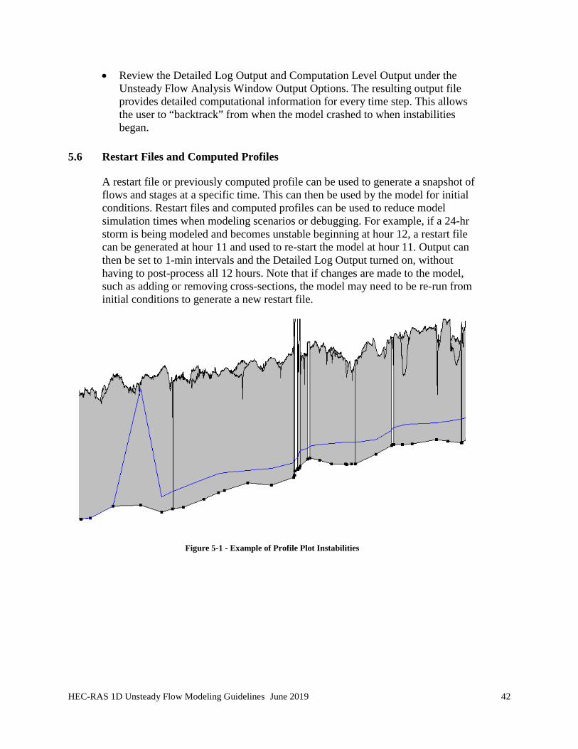
HEC-RAS 1D Unsteady Flow Modeling Guidelines June 2019 42
• Review the Detailed Log Output and Computation Level Output under the Unsteady Flow Analysis Window Output Options. The resulting output file provides detailed computational information for every time step. This allows the user to “backtrack” from when the model crashed to when instabilities began.
5.6 Restart Files and Computed Profiles
A restart file or previously computed profile can be used to generate a snapshot of flows and stages at a specific time. This can then be used by the model for initial conditions. Restart files and computed profiles can be used to reduce model simulation times when modeling scenarios or debugging. For example, if a 24-hr storm is being modeled and becomes unstable beginning at hour 12, a restart file can be generated at hour 11 and used to re-start the model at hour 11. Output can then be set to 1-min intervals and the Detailed Log Output turned on, without having to post-process all 12 hours. Note that if changes are made to the model, such as adding or removing cross-sections, the model may need to be re-run from initial conditions to generate a new restart file.
Figure 5-1 - Example of Profile Plot Instabilities

HEC-RAS 1D Unsteady Flow Modeling Guidelines June 2019 43
Figure 5-2 - Example of Hydrograph with Flow and Stage Instabilities
Instabilities begin

HEC-RAS 1D Unsteady Flow Modeling Guidelines June 2019 44
SECTION 6 - CONVERTING UNSTEADY FLOW TO STEADY FLOW
If a steady flow model is required, the unsteady flow model results can be used to guide the steady flow model flow change locations and HEC-HMS routings. HEC-HMS uses a single-point rating curve for its calculation and cannot model a looped rating curve as is commonly caused by backwater conditions prominent on many streams in Harris County. Due to this inability, weir sizes and coefficients used in modeling mitigation basins in HEC-HMS may not necessarily reflect the true proposed conditions geometry as represented in the unsteady flow model. The goal is to replicate to the extent possible the results of the unsteady flow model in the HEC-HMS model and steady flow HEC-RAS models that are used for regulatory purposes. The modeler must document the differences in parameters used in HEC-HMS to replicate the unsteady flow model results in the No Adverse Impact Report. The following is a simplified example of a conversion from unsteady to steady flow demonstrating one method that can be used for developing a steady flow file using results from the unsteady flow model as a guide:
1. Create a new, blank steady flow file. This will be used to import the peak flow from the unsteady flow model. This is required as HEC-RAS does not provide a summary table of peak flow rates. Note that HEC-RAS output tables present the flow at the maximum WSE which may or may not coincide with actual peak flow.
2. From the steady flow file menu, click “Set Location for DSS Connections” and assign DSS links to all cross-sections as shown below. This will allow modeler to determine where flow change of 5% or more occur indicating need for flow change in steady flow. Note that these locations must be selected as detailed output locations in the Unsteady Plan file to generate hydrographs in the output DSS file.
3. Once each location is added to the table, assign each a DSS link one-by-one to the unsteady flow model’s DSS file. See images on the following page.
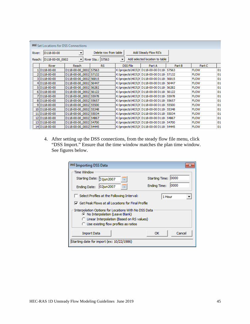
HEC-RAS 1D Unsteady Flow Modeling Guidelines June 2019 45
4. After setting up the DSS connections, from the steady flow file menu, click “DSS Import.” Ensure that the time window matches the plan time window. See figures below.
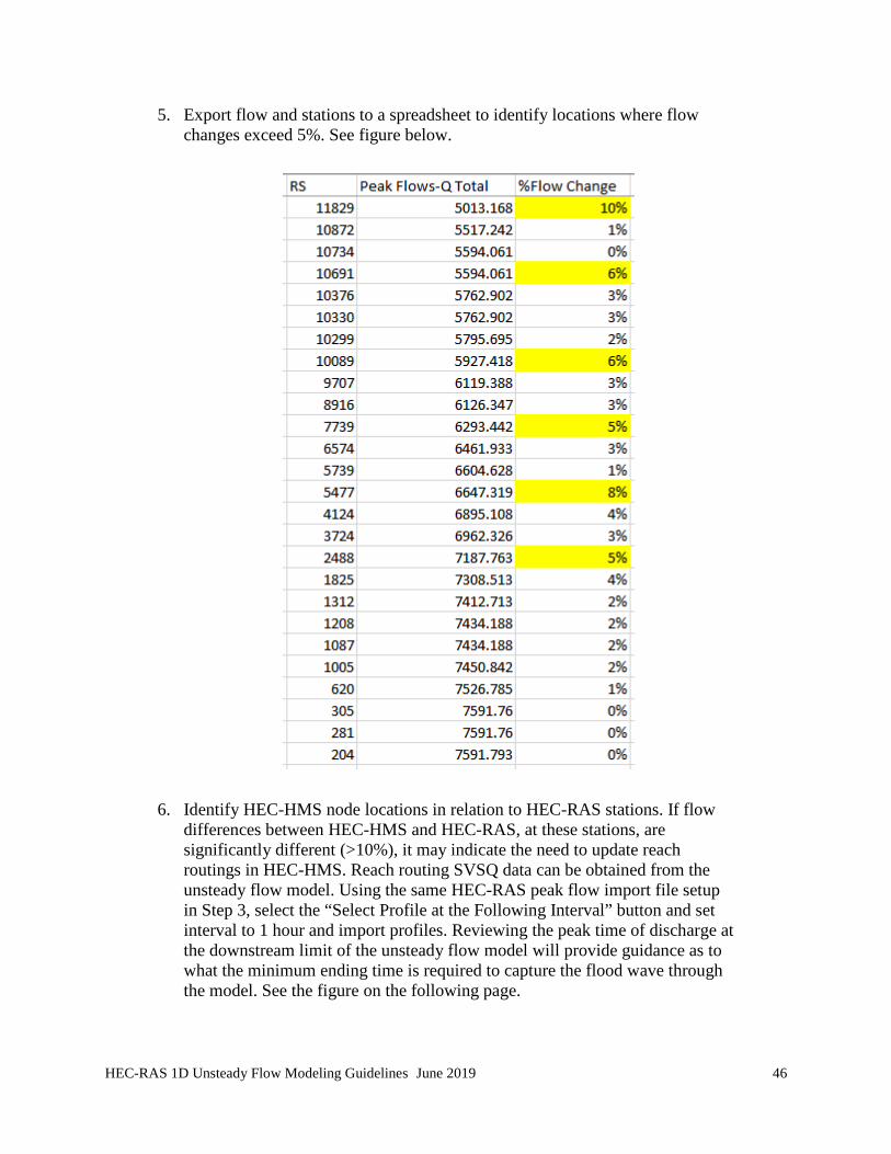
HEC-RAS 1D Unsteady Flow Modeling Guidelines June 2019 46
5. Export flow and stations to a spreadsheet to identify locations where flow changes exceed 5%. See figure below.
6. Identify HEC-HMS node locations in relation to HEC-RAS stations. If flow differences between HEC-HMS and HEC-RAS, at these stations, are significantly different (>10%), it may indicate the need to update reach routings in HEC-HMS. Reach routing SVSQ data can be obtained from the unsteady flow model. Using the same HEC-RAS peak flow import file setup in Step 3, select the “Select Profile at the Following Interval” button and set interval to 1 hour and import profiles. Reviewing the peak time of discharge at the downstream limit of the unsteady flow model will provide guidance as to what the minimum ending time is required to capture the flood wave through the model. See the figure on the following page.

HEC-RAS 1D Unsteady Flow Modeling Guidelines June 2019 47
Once the multiple flow profiles have been imported and the steady flow model ran, select from the main project window File -> Export to HEC-DSS -> Storage Outflow and assign the upstream and downstream stations for the reach(s) and export volume outflow data.
Open the DSS file from HEC-RAS and plot the exported curve. Use the measure tool in HEC-RAS to approximate the upper points of the graph and insert the computed SVSQ into the appropriate HEC-HMS reach. It is likely the graph will have an irregular profile due to backwater effects. By tracing the upper limits of the graph a reasonable representation of unsteady flow routing results through the reach can often be obtained. See the figure on the following page.

HEC-RAS 1D Unsteady Flow Modeling Guidelines June 2019 48
7. Once reasonable agreement in flows are achieved between unsteady and HEC-HMS nodes, use the “Growth” function in excel to interpolate flow changes at the previously identified >5% flow change locations.

HEC-RAS 1D Unsteady Flow Modeling Guidelines June 2019 49
8. Comparing results of the unsteady to steady flow model flows it is found that the two are generally within 10% of each other. For this example, the peak WSE computed by the two models is also within a generally acceptable agreement. If model results are being used for design purposes, the higher WSE of the two models should be used for setting critical elevations. See figure below and on the following page.
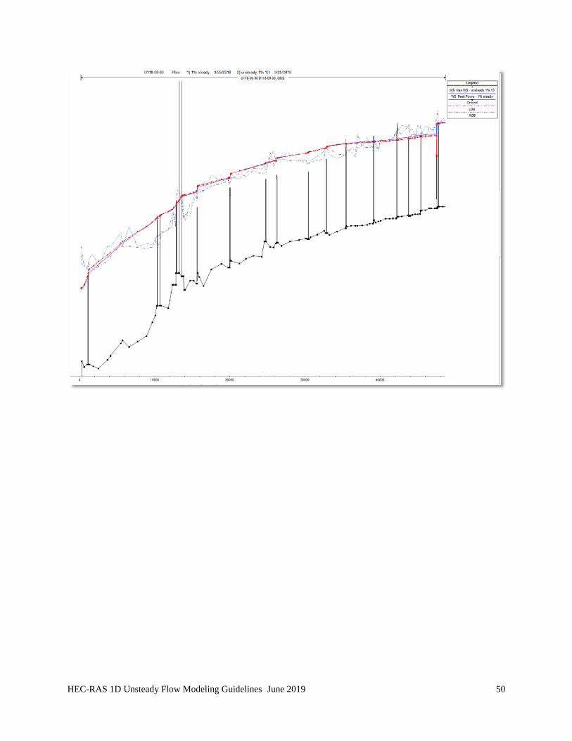
HEC-RAS 1D Unsteady Flow Modeling Guidelines June 2019 50

HEC-RAS 1D Unsteady Flow Modeling Guidelines June 2019 51
SECTION 7 - MODEL OUTPUTS & DELIVERABLES
The following sections summarize the model outputs and deliverables required when a HEC-RAS 1D unsteady flow model is submitted to the HCFCD for review. These outputs and deliverables are in addition to any information required by the HCFCD PCPM. Failure to supply the information in the formats discussed will result in rejection of the submittal. The following is a summary of the required model outputs and deliverables (see following sections for additional details):
• Model files summary table
• Boundary conditions summary table
• HEC-DSS summary table
• Watershed Overview exhibit
• Model Overview exhibit
• Summary of model revisions
• Computation Options and Tolerances screenshot
• HEC-RAS river cutline vs. reach length summary table
• Summary of HEC-RAS runtime messages and explanation of any errors and/or warnings
In addition to the required model outputs and deliverables, the following requires approval by HCFCD and, if used, should be noted and discussed in the report.
• Restart file (for initial conditions)
• Upstream boundary conditions (other than flow)
• Downstream boundary conditions (other than normal depth)
• The following internal boundary conditions: o Rating Curves
o Gate opening time series
o Elevation controlled gates
o Navigation dams
o Pump stations
o Groundwater interflows
o Stage
• Diversion rating curve(s)
• Lateral weir crest shape (if other than Broad Crested)

HEC-RAS 1D Unsteady Flow Modeling Guidelines June 2019 52
• Linear Routing method (when used for Lateral Weirs)
• Bridge / culvert Options (if other than the defaults)
• The following computation options:
o Lateral and inline structure flow stability factors (if other than 3.0)
o Weir and gate flow submergence decay exponents (if other than 3.0)
o Friction slope methods (if other than the defaults)
o Mixed flow Froude number factor (if other than the defaults)
o Mixed flow Froude number threshold (if other than the defaults)
Although the following do not require approval by the HCFCD, note and discuss in the report if any of the following were used:
• Pilot Channels
• Lidded cross-sections (with or without a Priessmann slot)
• Skew(s) (and if used, include skew summary table)
• Inline weir(s) (if only used for stability)
• Storage Area junction method
• Levee features
Lastly, double check that the following (often overlooked) guidelines were met:
• Cross-section HTAB starting elevations equal to the cross-section invert
• Cross-section HTAB increments of 0.1-ft or less
• Cross-section HTAB points sufficient to extend at least 2-ft above the 500-year WSE
• Bridge HTABs set properly, including tailwater maximum elevation and maximum flow
• Ineffective areas set to permanent or non-permanent appropriately
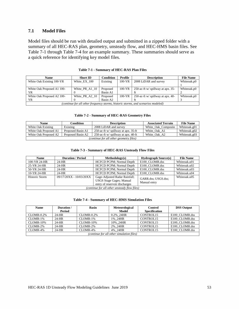
HEC-RAS 1D Unsteady Flow Modeling Guidelines June 2019 53
7.1 Model Files
Model files should be run with detailed output and submitted in a zipped folder with a summary of all HEC-RAS plan, geometry, unsteady flow, and HEC-HMS basin files. See Table 7-1 through Table 7-4 for an example summary. These summaries should serve as a quick reference for identifying key model files.
Table 7-1 - Summary of HEC-RAS Plan Files
Name Short ID Condition Profile Description File Name White Oak Existing 100-YR White_EX_100 Existing 100-YR 2008 LiDAR and survey Whiteoak.p0
1 White Oak Proposed A1 100-YR
White_PR_A1_100
Proposed Basin A1
100-YR 250-ac-ft w/ spillway at apx. 35-ft
Whiteoak.p02
White Oak Proposed A2 100-YR
White_PR_A2_100
Proposed Basin A2
100-YR 250-ac-ft w/ spillway at apx. 40-ft
Whiteoak.p03
(continue for all other frequency storms, historic storms, and scenarios modeled)
Table 7-2 - Summary of HEC-RAS Geometry Files
Name Condition Description Associated Terrain File Name White Oak Existing Existing 2008 LiDAR and survey White_Oak_Composite Whiteoak.g01 White Oak Proposed A1 Proposed Basin A1 250-ac-ft w/ spillway at apx. 35-ft White_Oak_A1 Whiteoak.g02 White Oak Proposed A2 Proposed Basin A2 250-ac-ft w/ spillway at apx. 40-ft White_Oak_A2 Whiteoak.g03
(continue for all other geometry files)
Table 7-3 - Summary of HEC-RAS Unsteady Flow Files
Name Duration / Period Methodology(s) Hydrograph Source(s) File Name 100-YR 24-HR 24-HR HCFCD PCPM; Normal Depth E100_CLOMR.dss Whiteoak.u01 25-YR 24-HR 24-HR HCFCD PCPM; Normal Depth E100_CLOMR.dss Whiteoak.u02 50-YR 24-HR 24-HR HCFCD PCPM; Normal Depth E100_CLOMR.dss Whiteoak.u03 10-YR 24-HR 24-HR HCFCD PCPM; Normal Depth E100_CLOMR.dss Whiteoak.u04 Historic Storm 09/17/20XX - 10/03/20XX Gage-Adjusted Radar Rainfall;
USGS Stage Gages; Manual entry of reservoir discharges
GARR.dss; USGS.dss; Manual entry
Whiteoak.u05
(continue for all other unsteady flow files)
Table 7-4 - Summary of HEC-HMS Simulation Files
Name Duration / Period
Basin Meteorological Model
Control Specification
DSS Output
CLOMR-0.2% 24-HR CLOMR-0.2% 0.2%_24HR CONTROL15 E100_CLOMR.dss CLOMR-1% 24-HR CLOMR-1% 1%_24HR CONTROL15 E100_CLOMR.dss CLOMR-10% 24-HR CLOMR-10% 10%_24HR CONTROL15 E100_CLOMR.dss CLOMR-2% 24-HR CLOMR-2% 2%_24HR CONTROL15 E100_CLOMR.dss CLOMR-4% 24-HR CLOMR-4% 4%_24HR CONTROL15 E100_CLOMR.dss
(continue for all other simulation files)

HEC-RAS 1D Unsteady Flow Modeling Guidelines June 2019 54
In addition, only the model files associated with relevant plans should be submitted. Working runs or alternative scenarios not relevant to the submittal should be deleted. Table 7-5 and Table 7-6 summarize the required model files that should be included in the submittal to support each project model set.
Table 7-5 - HEC-RAS Model Input Files Required
File Name Description
.prj One Project file
.p## One file for each Plan (.P01 to .P99)
.g## One file for each set of Geometry data (.G01 to .G99)
.f## One file for each set of Steady flow data (.F01 to .F99)
.u## One file for each set of Unsteady flow data (.U01 to .U99

HEC-RAS 1D Unsteady Flow Modeling Guidelines June 2019 55
Table 7-6 - HEC-RAS Model Output Files Required
File Name Description
.r## One Run file for each steady flow plan (.R01 to .R99) where ## is same as plan file number
.x## One Run file for each unsteady flow plan (.X01 to .X99) where ## is same as plan file number
.o## One Output file for each plan (.O01 to .O99) where ## is same as plan file number
.g##.hdf One corresponding HDF5 file for each geometry file (g##.hdf) where ## is same as geometry number
.p##.hdf One corresponding HDF5 file for each plan file (p##.hdf) where ## is same as plan file number
.b## One Unsteady Boundary Condition file for each plan file where ## is same as plan file number
.bco## One Plan Log Output file for each plan file where ## is same as plan file number
.c## One geometric pre-processor output file for each set of Geometry data where ## is same as geometry file number
.IC.o## One Initial Conditions file for each unsteady flow plan executed where ## is same as plan file number
.p##.blf One binary log file for each plan executed where ## is same as plan file number
.p##.rst One restart file (hot start) for each unsteady flow plan if option to write is turned on.
.dss Plan results in DSS format
.comp_msgs.txt Computational messages

HEC-RAS 1D Unsteady Flow Modeling Guidelines June 2019 56
7.2 Boundary Conditions
Boundary conditions must be summarized in a minimum of two types of tables for each unsteady flow file, as follows:
• HEC-RAS Boundary Conditions Summary
See Table 7-7 as an example. Columns ID through Comments must be exported from HEC-RAS via the Unsteady Flow Data window (see Figure 7-1). The table should then be appended in Excel with, at minimum, a HEC-DSS Part B Name and Notes column. The table provides the reviewer with a concise summary of all boundary conditions, associated flows and volumes, sources, and relevant information as noted by the modeler.
Figure 7-1 - Unsteady Flow Data Export Table
• HEC-RAS Boundary Conditions DSS Summary
See Table 7-8 as an example. HEC-RAS allows the modeler to extract a summary of boundary condition DSS paths. Within the Unsteady Flow Data editor, select the Options menu, then select DSS Pathname Summary Table. Include the table as a screenshot. Future versions of HEC-RAS may allow the user to export the table to Excel, in which case it can be submitted as a table.
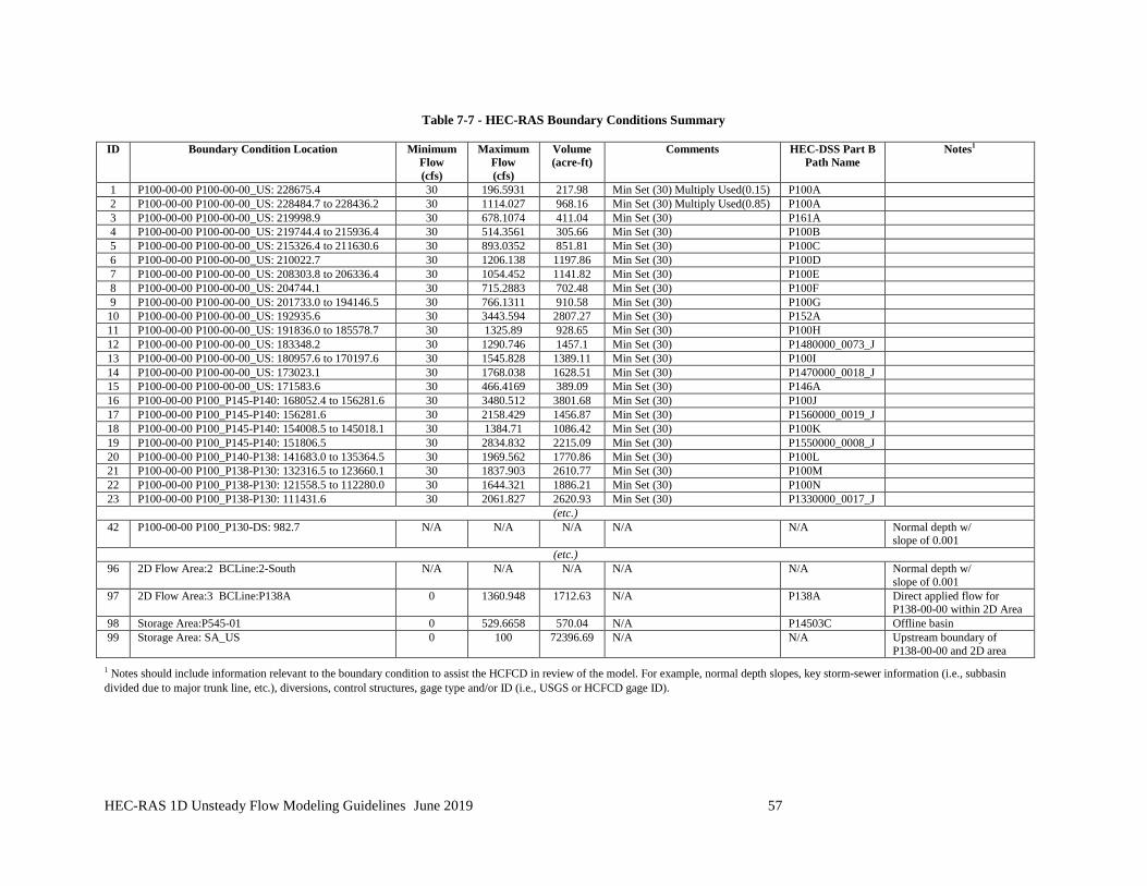
HEC-RAS 1D Unsteady Flow Modeling Guidelines June 2019 57
Table 7-7 - HEC-RAS Boundary Conditions Summary
ID Boundary Condition Location Minimum Flow (cfs)
Maximum Flow (cfs)
Volume (acre-ft)
Comments HEC-DSS Part B Path Name
Notes1
1 P100-00-00 P100-00-00_US: 228675.4 30 196.5931 217.98 Min Set (30) Multiply Used(0.15) P100A 2 P100-00-00 P100-00-00_US: 228484.7 to 228436.2 30 1114.027 968.16 Min Set (30) Multiply Used(0.85) P100A 3 P100-00-00 P100-00-00_US: 219998.9 30 678.1074 411.04 Min Set (30) P161A 4 P100-00-00 P100-00-00_US: 219744.4 to 215936.4 30 514.3561 305.66 Min Set (30) P100B 5 P100-00-00 P100-00-00_US: 215326.4 to 211630.6 30 893.0352 851.81 Min Set (30) P100C 6 P100-00-00 P100-00-00_US: 210022.7 30 1206.138 1197.86 Min Set (30) P100D 7 P100-00-00 P100-00-00_US: 208303.8 to 206336.4 30 1054.452 1141.82 Min Set (30) P100E 8 P100-00-00 P100-00-00_US: 204744.1 30 715.2883 702.48 Min Set (30) P100F 9 P100-00-00 P100-00-00_US: 201733.0 to 194146.5 30 766.1311 910.58 Min Set (30) P100G
10 P100-00-00 P100-00-00_US: 192935.6 30 3443.594 2807.27 Min Set (30) P152A 11 P100-00-00 P100-00-00_US: 191836.0 to 185578.7 30 1325.89 928.65 Min Set (30) P100H 12 P100-00-00 P100-00-00_US: 183348.2 30 1290.746 1457.1 Min Set (30) P1480000_0073_J 13 P100-00-00 P100-00-00_US: 180957.6 to 170197.6 30 1545.828 1389.11 Min Set (30) P100I 14 P100-00-00 P100-00-00_US: 173023.1 30 1768.038 1628.51 Min Set (30) P1470000_0018_J 15 P100-00-00 P100-00-00_US: 171583.6 30 466.4169 389.09 Min Set (30) P146A 16 P100-00-00 P100_P145-P140: 168052.4 to 156281.6 30 3480.512 3801.68 Min Set (30) P100J 17 P100-00-00 P100_P145-P140: 156281.6 30 2158.429 1456.87 Min Set (30) P1560000_0019_J 18 P100-00-00 P100_P145-P140: 154008.5 to 145018.1 30 1384.71 1086.42 Min Set (30) P100K 19 P100-00-00 P100_P145-P140: 151806.5 30 2834.832 2215.09 Min Set (30) P1550000_0008_J 20 P100-00-00 P100_P140-P138: 141683.0 to 135364.5 30 1969.562 1770.86 Min Set (30) P100L 21 P100-00-00 P100_P138-P130: 132316.5 to 123660.1 30 1837.903 2610.77 Min Set (30) P100M 22 P100-00-00 P100_P138-P130: 121558.5 to 112280.0 30 1644.321 1886.21 Min Set (30) P100N 23 P100-00-00 P100_P138-P130: 111431.6 30 2061.827 2620.93 Min Set (30) P1330000_0017_J
(etc.) 42 P100-00-00 P100_P130-DS: 982.7 N/A N/A N/A N/A N/A Normal depth w/
slope of 0.001 (etc.)
96 2D Flow Area:2 BCLine:2-South N/A N/A N/A N/A N/A Normal depth w/ slope of 0.001
97 2D Flow Area:3 BCLine:P138A 0 1360.948 1712.63 N/A P138A Direct applied flow for P138-00-00 within 2D Area
98 Storage Area:P545-01 0 529.6658 570.04 N/A P14503C Offline basin 99 Storage Area: SA_US 0 100 72396.69 N/A N/A Upstream boundary of
P138-00-00 and 2D area
1 Notes should include information relevant to the boundary condition to assist the HCFCD in review of the model. For example, normal depth slopes, key storm-sewer information (i.e., subbasin divided due to major trunk line, etc.), diversions, control structures, gage type and/or ID (i.e., USGS or HCFCD gage ID).

HEC-RAS 1D Unsteady Flow Modeling Guidelines June 2019 58
Table 7-8 - HEC-RAS Boundary Conditions DSS Summary

HEC-RAS 1D Unsteady Flow Modeling Guidelines June 2019 59
At a minimum, the following two exhibits must also be included to supplement the above tables:
• Watershed Overview Exhibit
See Figure 7-2 for an example. The Watershed Overview exhibit should provide an overview of the studied watershed with subbasins, HCFCD M3 and FEMA streams, major landmarks (e.g., highways, roads, etc.), and any other key feature relevant to the study (e.g., project site outline, major detention facilities, etc.).
• Model Overview Exhibit
See Figure 7-3 and Figure 7-4 for examples. The Model Overview exhibit should provide a detailed view of the HEC-RAS model while referencing the watershed, subbasins, and, if useful to the reviewer, HEC-HMS model components. The exhibit should allow the reviewer to visually relate the Boundary Conditions tables to the HEC-RAS model. If HEC-HMS subbasin runoff hydrographs are distributed along the HEC-RAS model using multipliers, it’s recommended that the subbasin shapefile be subdivided and shown in the exhibit. Other reference layers could also be added, such as relevant detention facilities and/or storm sewer systems. This will allow the reviewer to visually confirm boundary condition multiplier values and their rationale for dividing subbasins. Note that this level of detail may not always be warranted, particularly if the modeler approximated subbasin divides (i.e., assigned an approximate percentage, e.g., 75% and 25%, based on visual assessment of the subbasin and not detailed delineation). Figure 7-3 and Figure 7-4 should be considered examples, not templates, that the modeler can use when producing exhibits that best suit their project.
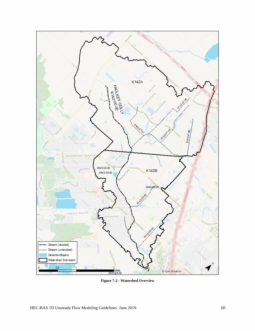
HEC-RAS 1D Unsteady Flow Modeling Guidelines June 2019 60
Figure 7-2 - Watershed Overview
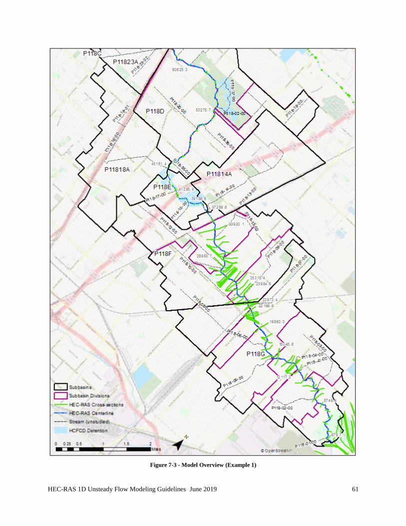
HEC-RAS 1D Unsteady Flow Modeling Guidelines June 2019 61
Figure 7-3 - Model Overview (Example 1)

HEC-RAS 1D Unsteady Flow Modeling Guidelines June 2019 62
Figure 7-4 - Model Overview (Example 2)
687.7
12117.3
33920.1 45161.4
60625.3

HEC-RAS 1D Unsteady Flow Modeling Guidelines June 2019 63
7.3 Additional Model Details
The following are additional model details that must be submitted.
• Summary of model revisions
Provide a summary of key revisions made to an existing model. Major changes should be noted explicitly (e.g., added bridge at Bayou Street, added offline detention basin at Mercer Park, lowered project site channel n value from existing grass to concrete, etc.), while broad, general revisions can be discussed in general (e.g., added breaklines to reflect major highways, revised n values to reflect 2018 land use). Include a plan view exhibit showing new and/or revised cross-sections through the project site. This summary should be presented as a narrative versus a detailed list or table of changes in order to help guide the reviewer (although tables can be included to summary changes).
• Computation Options and Tolerances
The HEC-RAS Computation Options and Tolerances menu should be included as a screenshot for each unsteady flow plan. See Figure 7-5 as an example.
• HEC-RAS River Cutline vs. Reach Lengths
A comparison should be made between the HEC-RAS river reach cutlines and the total reach length of the river reach. See Table 7-9 for an example. The cutline length can be computed in the Geometry window by selecting the GIS Tools menu, Reach Invert Lines Table, and then clicking the Compute Line Length button. To compute the total reach length, in the Geometry window select the Tables menu and Reach Lengths. From the table that appears, export the channel reach length column to Excel and sum the total reach length.
• Summary of Skew Angles
The location and angle of any skews used in the model should be summarized (see Table 7-10 for a template).
• HEC-RAS Runtime Messages
The HEC-RAS Runtime Messages should be copied and pasted for each plan. Any WSE errors greater than 0.1-ft and the modeler’s justification should be discussed. The runtime messages should be copy and pasted (not taken as a screenshot) as shown in Figure A-5. The modeler can refer to errors by referencing the messages or can insert commentary directly in the copy and pasted message. If inserting commentary directly, ensure that the responses are clearly distinguishable from the runtime message text.
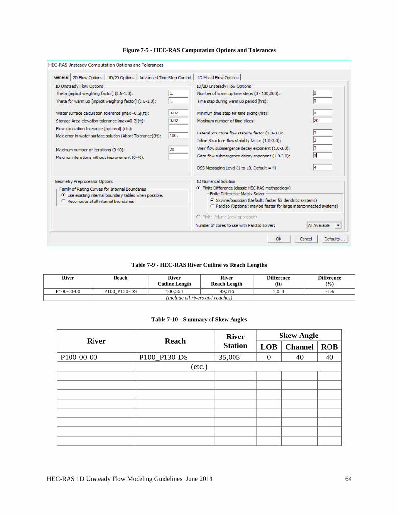
HEC-RAS 1D Unsteady Flow Modeling Guidelines June 2019 64
Figure 7-5 - HEC-RAS Computation Options and Tolerances
Table 7-9 - HEC-RAS River Cutline vs Reach Lengths
River Reach River Cutline Length
River Reach Length
Difference (ft)
Difference (%)
P100-00-00 P100_P130-DS 100,364 99,316 1,048 -1% (include all rivers and reaches)
Table 7-10 - Summary of Skew Angles
River Reach River Station
Skew Angle LOB Channel ROB
P100-00-00 P100_P130-DS 35,005 0 40 40 (etc.)

HEC-RAS 1D Unsteady Flow Modeling Guidelines June 2019 65
Figure 7-6 - HEC-RAS Runtime Messages
Plan: '100YR-H100' (H100.p01) Simulation started at: 25Jul2018 01:16:09 PM Using 64 Bit Computation Engines Performing Unsteady Flow Simulation HEC-RAS 5.0.5 June 2018 Maximum adaptive timestep = 01:00.0 Minimum adaptive timestep = 00:15.0 Initial adaptive timestep = 00:30.0 Initial Backwater, Split flow optimization, iteration 1 Initial Backwater, Split flow optimization, iteration 2 Initial Backwater, Split flow optimization, iteration 3 Initial Backwater, Split flow optimization, iteration 4 Maximum iterations of 20 RS (or Cell) WSEL ERROR 01JUN2007 01:44:00 H1030000 H1030000 19519 33.73 0.023 01JUN2007 01:44:15 H100-00-00 H1180000 130 32.98 0.150 01JUN2007 01:44:30 H100-00-00 H1180000 830.00 35.55 0.062 01JUN2007 01:44:45 H100-00-00 H1180000 130 32.91 0.105 01JUN2007 01:45:00 H100-00-00 H1180000 130 32.95 0.120 01JUN2007 01:45:15 H100-00-00 H1180000 130 32.96 0.118 01JUN2007 01:45:30 H100-00-00 H1180000 130 32.95 0.120 01JUN2007 01:45:45 H100-00-00 H1180000 130 33.00 0.127 01JUN2007 01:46:00 H100-00-00 H1180000 130 32.94 0.128 01JUN2007 01:46:15 H100-00-00 H1180000 130 32.98 0.140 01JUN2007 01:46:30 H100-00-00 H1180000 130 32.98 0.144 01JUN2007 01:46:45 H100-00-00 H1180000 130 32.97 0.144 01JUN2007 01:47:00 H100-00-00 H1180000 130 32.95 0.156 01JUN2007 01:47:15 H100-00-00 H1180000 130 33.04 0.155 01JUN2007 01:47:30 H100-00-00 H1180000 130 32.90 0.137 01JUN2007 01:47:45 H100-00-00 H1180000 130 33.00 0.169 01JUN2007 01:48:00 H100-00-00 H1180000 130 33.03 0.158 01JUN2007 01:48:15 H100-00-00 H1180000 130 33.04 0.155 01JUN2007 01:48:30 H100-00-00 H1180000 130 33.04 0.153 01JUN2007 01:48:45 H100-00-00 H1180000 130 33.18 0.143 01JUN2007 01:49:00 H100-00-00 H1180000 130 33.06 0.122 01JUN2007 01:49:45 H100-00-00 H1180000 130 33.13 0.163 01JUN2007 09:27:15 H100-00-00 H1100000 82.3 34.19 0.054 Writing Results to DSS The maximum xsec wsel error was 0.169 H100-00-00 H1180000 130 at 01JUN2007 01:47:45 The maximum storage area wsel error was 0.023 h103_us_junct at 01JUN2007 01:44:00 Finished Unsteady Flow Simulation Reading Data for Post Process Computations Summary Computation Task Time(hh:mm:ss) Completing Geometry(64) 4 Preprocessing Geometry(64) 5 Unsteady Flow Computations(64) 1:13:55 Post-Processing(64) 1:21 Computing Maps(64) 1 Complete Process 1:15:31
Response: The maximum iterations and errors occur during low flow conditions only. These do not affect peak water surface elevations or flows occurring approximately 14 hours later.