5

Chapter 2: Satellite instruments

Satellite remote sensors are instruments designed to obtain information on the atmospheric composition through the analysis of data acquired without direct contact with the atmosphere. While remote sensors can also be employed from the ground, balloon or aircra�, on satellites they provide a unique global view with a more comprehensive geographical coverage and regular observations. Satellite instruments can o�er total column or height-resolved measurements. For this purpose, satellite instruments take advantage of di�erent interactions of radiation with the atmosphere (e.g., absorption, emission or scattering) and detect wavelengths throughout the electromagnetic spectrum. Disadvantages of satellite instruments are that they are o�en expensive, can be high risk, require complex space-quali�ed instrumentation, and have limited lifetimes.

In this chapter, Section 2.1 presents a general discussion of the satellite measurement techniques and orbit types relevant for the instruments participating in the SPARC Data Initiative. More detailed descriptions of the speci�c instruments, including information on retrieval processes, are given in Section 2.2.

2.1 Satellite measurement techniques

�e satellite instruments participating in the SPARC Data Initiative are all passive sensors. Passive sensors detect natural radiation emitted from an external source (i.e., the sun or stars) or by the atmosphere itself. Active sensors, on the other hand, emit high-energy radiation themselves and detect what is re�ected back from the atmosphere (e.g., LIDARs). In this section, general characteristics of various passive remote sensing techniques are described in terms of measurement geometry and wavelength coverage, however the scope is limited to concepts relevant to this study.

Table 2.1 provides a classi�cation of the instruments participating in the SPARC Data Initiative according to both categories (observation geometry and wavelengths), which are explained in more detail in Sections 2.1.1 and 2.1.2, respectively.

2.1.1 Classi�cation by observation geometry

Satellite instruments can be classi�ed according to their observation geometry into limb-viewing or nadir-viewing sounders. Limb sounders look tangentially through the

atmosphere, while nadir sounders have a downward-viewing observation geometry, pointing towards the Earth’s surface. Limb geometries are the natural choice for stratospheric measurements because the signal is not masked by the denser tropospheric signal, the long ray-path through the atmosphere provides large sensitivity to species with low atmospheric concentrations, and the variation of the observation angle allows vertical scanning of the atmosphere. As a result, altitude information on the observed atmospheric state variables can be obtained at high vertical resolution, while the horizontal resolution is limited. For tropospheric observations, limb measurements are more challenging because of the saturation of measured radiances and the opaqueness of the troposphere due to the presence of clouds, humidity, and generally larger density. For many aspects of tropospheric sounding, nadir sounders are advantageous, due to their small horizontal footprint.

In the following, limb-viewing sounders are further classi�ed according to their measurement modes, which are based on emission, scattering, solar occultation, and stellar occultation. In parts of the satellite observation community the term ‘limb sounding’ is reserved for limb emission and limb scattering measurements, but here the term is used in a more general sense, including the occultation geometry. A description of the nadir emission technique is also provided.

Limb emission

Emission measurements in limb geometry record the signal that is emitted along a horizontal path through the atmosphere and is partly absorbed on its way between the emitting air parcel and the observer (see Figure 2.1). Variation of the elevation angle of the line-of-sight (LOS) allows altitude-resolved temperature and composition measurements from approximately cloud-top height to the thermosphere. In turn, the horizontal resolution is limited to ~300 km unless corrections for LOS gradients are applied, or tomography is used. Since the Planck function at terrestrial temperatures is very low for wavelengths shorter than about 2.5 µm, limb emission measurements are, at least under conditions of local thermodynamic equilibrium, feasible only at wavelengths larger than this threshold, i.e., in the mid-infrared to the microwave spectral region. At these wavelengths, atmospheric scattering is negligible except for clouds and large aerosol particles. Since, in contrast to occultation measurements (see

6 Chapter 2: Satellite instruments

below), no direct illumination source is needed, emission measurements can be obtained during both day and night. Depending on the orbit of the platform, measurements can be performed globally with dense spatial coverage, and the azimuth angle can be arbitrarily chosen as long as the Sun is avoided. A disadvantage of the emission technique compared to occultation measurements is the relatively small signal to noise ratio, which is caused by the faint signal of atmospheric emission. Calibration and determination of the exact elevation angle of the LOSs are crucial to avoid propagation of related errors onto the retrieved trace gas abundance pro�les. Within the SPARC Data Initiative, the limb emission technique is used by Aura-MLS, HIRDLS, LIMS, MIPAS, SMILES, SMR, and UARS-MLS.

Solar occultation

Solar occultation instruments record radiance emitted by the Sun and attenuated along a horizontal ray-path through the atmosphere by extinction, i.e., absorption and scattering (see Figure 2.2). Similar to the limb emission measurements, altitude-resolved information is obtained by variation of the elevation angle of the LOS. However, in contrast to limb emission where the measurement geometry can be freely chosen, the geometry is de�ned by the position of the Sun with respect to that of the satellite and the Earth. Measurements in occultation geometry can only be performed during the sunrise and sunset as seen from the satellite, i.e., two times per orbit, which results in

a limited global coverage and greatly reduced data density (compared to an emission sounder). On the other hand, the Sun provides a large radiance signal, allowing highly precise measurements even at shorter wavelengths. Occultation measurements are usually performed at wavelengths from the UV to the mid-IR. �ese measurements are self-calibrating in a sense that the division of atmospheric spectra by direct Sun (e.g., exo-atmospheric) spectra yields transmission spectra. Within the SPARC Data Initiative, solar occultation is represented by ACE-FTS, ACE-MAESTRO, HALOE, POAM II/III, and SAGE I/II/III.

Stellar occultation

Stellar occultation measurements use the same concept as solar occultation measurements, except that stars act as the radiation source instead of the Sun (see Figure 2.2). Since multiple stars can be used, this results in a larger data density compared to that achieved by solar occultation. Night-time measurements are of better quality than daytime measurements because the scattered solar signal interferes with the target signal of the stars during daytime. �e useful spectral range is limited to wavelengths below about 1  µm. At longer wavelengths terrestrial thermal emission interferes with the stellar signal. Weak stellar radiation and scintillations from atmospheric irregularities are particular challenges of stellar occultation techniques. Within the SPARC Data Initiative, stellar occultation is represented by GOMOS.

Table 2.1: I n s t r u m e n t s classi�ed according to ob-servation geometry and wavelength categories. Only instruments partici-pating in the SPARC Data Initiative, and the measure-ment modes considered, are listed.

Microwave / Sub-mm100 μm - 10 cm

Mid-IR2.5 - 20 μm

Near-IR0.8 - 2.5 μm

VIS / UV< 0.8 μm

Limb emission

UARS-MLSAura-MLS

SMRSMILES

MIPASHIRDLS

LIMS

Solar occultation

ACE-FTSHALOE

POAM II/IIISAGE I/II/III

POAM II/IIISAGE I/II/III

ACE-MAESTRO

Stellar occultation

GOMOS

Limb scattering

SCIAMACHY SCIAMACHYOSIRIS

Nadir emission

TES

LOS

Earth

Instrument

Atmosphere

Figure 2.1: Limb emission observation geometry.The instrument measures radiation emitted by the atmosphere along the LOS.

7Chapter 2: Satellite instruments

Limb scattering

�e radiance received by limb scattering instruments consists of photons originating from the Sun and scattered into the �eld-of-view of the instrument (see Figure 2.3). �e information on the atmospheric state is provided by the scattering itself, or by the absorption of scattered photons along their way through the atmosphere. In contrast to the measurement techniques discussed above, the ray-path is not de�ned by the measurement geometry, but is scattered by the atmosphere into the LOS of the instrument. As for all measurement techniques using the Sun as the source of the signal, measurements are only possible during daylight. On the sunlit part of the globe, good spatial coverage is achieved. �e vertical resolution is similar to that of limb emission and solar occulation instruments. Measurements are made in the UV to the near-infrared range where scattering is relevant. Within the SPARC Data Initiative, limb scattering is represented by OSIRIS and SCIAMACHY.

Nadir emission

Nadir observations are measurements for which the LOS points down to the surface of the Earth. �e signal received by nadir emission instruments can contain photons emitted by the Earth’s surface or atmosphere and transmitted through the atmosphere. In contrast to limb measurements, for which vertically resolved measurements are achieved simply by variation of the elevation angle of the LOS, the altitude information of nadir observations is given by pressure broadening of spectral lines and by varying opacity at di�erent wavelengths. While the altitude resolution is far inferior to that of limb sounders, the horizontal resolution is better, and allows more measurements between clouds that can penetrate lower into the troposphere. �e LOS

through the atmosphere is shorter than in limb sounding, which reduces sensitivity to low abundance species but also reduces opacity problems. Infrared nadir sounding is possible during both day and night, but thermal contrast has an impact on altitude resolution and sensitivity to the abundance of species in the lower troposphere. Nadir infrared measurements require on-board blackbody calibration and a space view for cold space calibration measurements. Uncertainties in surface emissivity can complicate the retrieval process. Within the SPARC Data Initiative, nadir emission measurements are represented by TES. Note that TES is the only nadir-viewing instrument considered by the SPARC Data Initiative. TES evaluations presented in this report account for the relatively broad averaging kernel of the instrument and serve as an example for the more comprehensive comparisons that would be needed when considering nadir instruments (such instruments include, for example SBUV, TOMS, and MOPITT).

2.1.2 Classi�cation by wavelengths

�e di�erent instruments can, in addition to the classi�cation by observation geometry, be classi�ed according to the spectral range in which they operate. Wavelengths used for atmospheric composition measurements range from the microwave to the ultraviolet spectral region. Instruments contributing to the SPARC Data Initiative include both radiometers, which measure a signal spectrally integrated over certain frequency bands, and spectrometers, which provide spectrally resolved measurements. Better spectral resolution allows measurement of trace gas species with weaker spectral signatures. On the other hand, the advantage of lower spectral resolution is a higher signal-to-noise ratio for single measurements, which helps to provide better spatial resolution.

Sun/Star

Atmosphere

LOS

EarthInstrument

Figure 2.2: O c c u l t a -tion observation ge-ometry. The instrument points at the radiation source (the Sun or a star) and measures the radiation attenuated along the LOS.

Sun

Atmosphere

LOS

Earth

Instrument

Figure 2.3: Limb scatter-ing observation geometry. The instrument measures radiation emitted by the Sun and scattered into the �eld-of-view.

8 Chapter 2: Satellite instruments

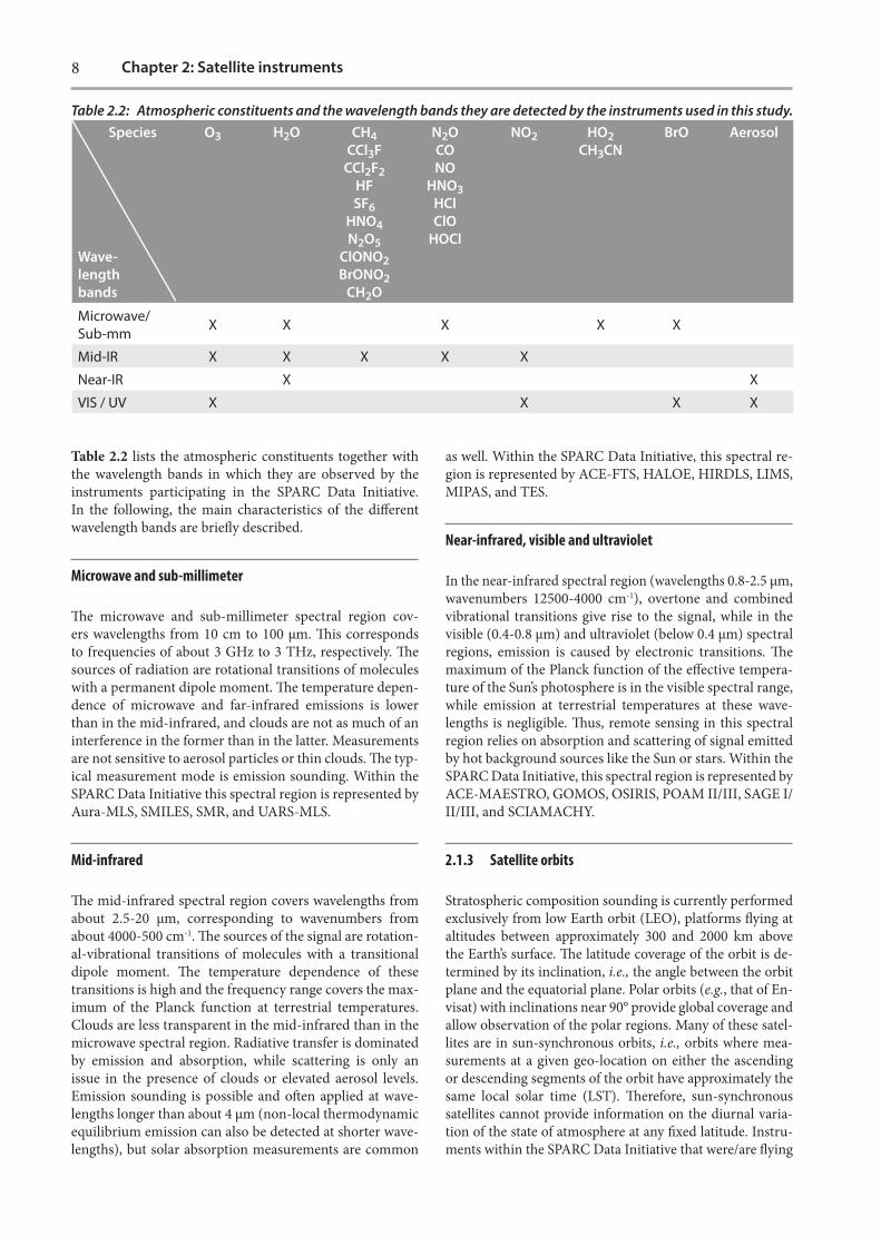
Table 2.2 lists the atmospheric constituents together with the wavelength bands in which they are observed by the instruments participating in the SPARC Data Initiative. In the following, the main characteristics of the di�erent wavelength bands are brie�y described.

Microwave and sub-millimeter

�e microwave and sub-millimeter spectral region cov-ers wavelengths from 10 cm to 100 μm. �is corresponds to frequencies of about 3 GHz to 3 THz, respectively. �e sources of radiation are rotational transitions of molecules with a permanent dipole moment. �e temperature depen-dence of microwave and far-infrared emissions is lower than in the mid-infrared, and clouds are not as much of an interference in the former than in the latter. Measurements are not sensitive to aerosol particles or thin clouds. �e typ-ical measurement mode is emission sounding. Within the SPARC Data Initiative this spectral region is represented by Aura-MLS, SMILES, SMR, and UARS-MLS.

Mid-infrared

�e mid-infrared spectral region covers wavelengths from about 2.5-20 μm, corresponding to wavenumbers from about 4000-500 cm-1. �e sources of the signal are rotation-al-vibrational transitions of molecules with a transitional dipole moment. �e temperature dependence of these transitions is high and the frequency range covers the max-imum of the Planck function at terrestrial temperatures. Clouds are less transparent in the mid-infrared than in the microwave spectral region. Radiative transfer is dominated by emission and absorption, while scattering is only an issue in the presence of clouds or elevated aerosol levels. Emission sounding is possible and o�en applied at wave-lengths longer than about 4 μm (non-local thermodynamic equilibrium emission can also be detected at shorter wave-lengths), but solar absorption measurements are common

as well. Within the SPARC Data Initiative, this spectral re-gion is represented by ACE-FTS, HALOE, HIRDLS, LIMS, MIPAS, and TES.

Near-infrared, visible and ultraviolet

In the near-infrared spectral region (wavelengths 0.8-2.5 μm, wavenumbers 12500-4000 cm-1), overtone and combined vibrational transitions give rise to the signal, while in the visible (0.4-0.8 μm) and ultraviolet (below 0.4 μm) spectral regions, emission is caused by electronic transitions. �e maximum of the Planck function of the e�ective tempera-ture of the Sun’s photosphere is in the visible spectral range, while emission at terrestrial temperatures at these wave-lengths is negligible. �us, remote sensing in this spectral region relies on absorption and scattering of signal emitted by hot background sources like the Sun or stars. Within the SPARC Data Initiative, this spectral region is represented by ACE-MAESTRO, GOMOS, OSIRIS, POAM II/III, SAGE I/II/III, and SCIAMACHY.

2.1.3 Satellite orbits

Stratospheric composition sounding is currently performed exclusively from low Earth orbit (LEO), platforms �ying at altitudes between approximately 300 and 2000 km above the Earth’s surface. �e latitude coverage of the orbit is de-termined by its inclination, i.e., the angle between the orbit plane and the equatorial plane. Polar orbits (e.g., that of En-visat) with inclinations near 90° provide global coverage and allow observation of the polar regions. Many of these satel-lites are in sun-synchronous orbits, i.e., orbits where mea-surements at a given geo-location on either the ascending or descending segments of the orbit have approximately the same local solar time (LST). �erefore, sun-synchronous satellites cannot provide information on the diurnal varia-tion of the state of atmosphere at any �xed latitude. Instru-ments within the SPARC Data Initiative that were/are �ying

Species

Wave-length bands

O3 H2O CH4CCl3F

CCl2F2HFSF6

HNO4N2O5

ClONO2BrONO2

CH2O

N2OCONO

HNO3 HClClO

HOCl

NO2 HO2CH3CN

BrO Aerosol

Microwave/Sub-mm X X X X X

Mid-IR X X X X X

Near-IR X X

VIS / UV X X X X

Table 2.2: Atmospheric constituents and the wavelength bands they are detected by the instruments used in this study.

9Chapter 2: Satellite instruments

on sun-synchronous satellites are Aura-MLS, GOMOS, HIRDLS, LIMS, MIPAS, OSIRIS, POAM II/III, SAGE III, SCIAMACHY, SMR, and TES. Non-sun-synchronous or-bits allow Earth observation at di�erent local times but lead to temporally varying datasets. �is can be an issue when creating climatologies, particularly for species with pro-nounced diurnal variations. Instruments within the SPARC Data Initiative that were/are �ying on non-sun-synchro-nous satellites/platforms are ACE-FTS, ACE-MAESTRO, HALOE, SAGE I/II, SMILES, and UARS-MLS.

2.2 Instrument and retrieval descriptions

�e satellite instruments participating in the SPARC Data Initiative are all passive sensors using a limb viewing ob-servation geometry with the exception of one nadir-view-ing sounder used for particular upper troposphere/lower stratosphere (UTLS) studies (see Section 4.27). �e mea-surement modes of the limb-viewing sounders (emission, scattering, solar occultation, and stellar occultation) deter-mine data coverage and sampling density.

Retrieval processes include a so-called forward model and an inversion algorithm. �e forward model computes radi-ances that would be observed given a state vector of atmo-spheric composition and temperature pro�les. �e inver-sion algorithm then “inverts” these calculations and solves for an atmospheric state from a given set of radiance ob-servations. In many cases (ACE-FTS, Aura-MLS, HALOE, HIRDLS, LIMS, MIPAS, SMR, TES, UARS-MLS), initial retrievals of temperature and pressure are performed us-ing observations of molecules whose abundances are well known (usually CO2 in the infrared and O2 in the micro-wave). Temperature and pressure can be retrieved as sepa-rate products if the emission lines are strong enough (e.g., SMILES, SMR). Some instruments (e.g., OSIRIS, SAGE II, SCIAMACHY) rely on meteorological analyses for temper-ature pro�le information. In either case, accurate knowl-edge of tangent altitude/pressure is required for limb mea-surements.

Uncertainties are typically provided by the operational re-trieval systems, but they generally do not include system-atic e�ects such as the propagation of spectroscopic uncer-tainties. Beyond such uncertainties, retrieval constraints (e.g., smoothing) a�ect the altitude resolution and lead to an imperfect representation of the true atmospheric state. Available validation information is provided separately for each molecule in Chapter 4.

In the following, the di�erent instruments together with their retrieval processes are described, in order of their launch date, with the earliest instrument �rst.

2.2.1 LIMS on Nimbus 7

Nimbus 7 was launched on October 24, 1978, and carried a number of instruments for making measurements of the

state of the middle atmosphere. �e Limb Infrared Monitor of the Stratosphere (LIMS) experiment was a limb-infrared sounder, focused on measurements of temperature, O3, and those species that a�ect ozone (H2O, NO2 and HNO3) [see Gille and Russell, 1984]. Nimbus 7 was in a sun-synchro-nous orbit with a noon and midnight equator crossing time. However, LIMS was designed to look o�-plane, so that the measurements were made near 1pm and 11pm local time at equator crossing. �e resulting sampling pattern can be found in Figure 10 of Gille and Russell [1984]. �e tempera-ture and ozone pro�les extend from cloud-top to near the mesopause, while the pro�les of H2O, HNO3, and NO2 are restricted to the stratosphere, due to their signal-to-noise (S/N) limitations. �e cryogen gases that were used to cool the detectors only lasted until May 28, 1979, as planned. �us, the LIMS dataset extends for about 7.5 months and consists of daily, orbital pro�les from about 64°S to 84°N latitude. �e data were processed with a Version 5 algo-rithm and archived in 1982 at NASA Goddard. More re-cently, the algorithm was revised to Version 6, and new re-trievals were conducted and archived at the Mirador site of the Goddard Earth Sciences and Data Information Services Center (GES DISC) or at http://daac.gsfc.nasa.gov and can be downloaded via �p from there. A separate LIMS website exists at http://www.gats-inc.com/projects.html#lims for viewing daily plots of the data. Descriptions of the qual-ity of the Version 6 temperature, O3, H2O, and HNO3 and NO2 can be found in Remsberg et al. [2004, 2007, 2009, and 2010], respectively.

Retrievals for the LIMS V6 temperature versus pressure (or T(p)) pro�les are described in Remsberg et al. [2004] and references therein. �e algorithm uses a top-down, onion-peeling approach and iterates to achieve a match of the cal-culated and measured radiances for its wide and narrow CO2 radiometer channels in the 15-μm region. A constant CO2 mixing ratio pro�le was assumed for the forward radiance models. Radiance pro�les for the LIMS species channels are registered with pressure according to the associated T(p) pro�les, and their forward models account for the retrieved temperatures. Level 2 pro�les of the temperature and species volume mixing ratio (VMR) are tabulated at 18 levels per de-cade of pressure or at a spacing of 0.88 km. �ey have an ef-fective vertical resolution of 3.7 km. �e retrieval algorithm for NO2 accounts for interfering radiances from H2O, CH4, and the oxygen continuum in the 6-7 μm region. �e algo-rithm for HNO3 accounts for interfering radiances from the primary CFC molecules and from aerosol emissions in the 11-µm region.

2.2.2 SAGE I on AEM-B, SAGE II on ERBS, and SAGE III on Meteor-3M

�e Stratospheric Aerosol and Gas Experiment (SAGE) series of instruments consists of four instruments including the Stratospheric Aerosol Measurement (SAM  II) that span the period from 1978 through 2005. All of the instruments use solar occultation to measure attenuated solar radiation through the Earth’s limb during satellite

10 Chapter 2: Satellite instruments

sunrise and sunset. �e �rst instrument in the series, SAM II on-board Nimbus 7 (1978-1993), consisted of a single 1000-nm aerosol channel with measurements restricted to high latitudes (>53° in both hemispheres). Note, SAM II is not included in the evaluations of this report. SAGE I on-board AEM-B (1979-1981) consisted of four measurement channels (corresponding to wavelengths of 385, 450, 600, and 1000 nm), which were used to infer aerosol extinction pro�les at two wavelengths (450 and 1000 nm) and O3 and NO2 concentration pro�les. SAGE II on-board ERBS (1984-2005) made measurements at seven wavelengths (385, 448, 452, 525, 600, 940, and 1020 nm) from which O3, NO2, H2O and aerosol extinction at four wavelengths (385, 452, 525, and 1020 nm) were retrieved [McCormick et al., 1989]. SAGE III on-board the Russian Meteor-3M satellite was launched on December 2001 and remained operational into December 2005. It used an 800 element Charged Coupled Device (CCD) linear array

detector to provide continuous spectral coverage between 280 and 1040 nm. An additional single photodiode at 1550 nm was used for aerosol extinction measurements. �e SAGE III measurements at 87 channels between 285  and 1545 nm were used to infer vertical pro�les of O3, NO2, H2O, and aerosol extinction at nine wavelengths (285, 448, 521, 602, 676, 755, 868, 1019, and 1545 nm) [�omason and Taha, 2003].

Both SAGE I and II instruments were in inclined (~57°) orbits that permitted near-global coverage over the course of 30 to 40 days (see Figure 2.4). �ere are 15 sunrise and 15 sunset measurements each day that cover a narrow latitude band and are separated by ~24° in longitude. Un-like SAGE I and II, where sunrise and sunset measure-ments alternatively observe the Northern and Southern Hemispheres, all SAGE III sunrise measurements occur in the Southern Hemisphere (30°S to 60°S) while all sunset

Figure 2.4: Sampling pattern and resulting sample density for SAGE II (left) and SAGE III (right). Note, SAGE I provided similar geographical and temporal sampling as SAGE II. For SAGE III, sunrise measurements occur in the Southern Hemi-sphere, and sunset events occur in the Northern Hemisphere.

latit

ude

month

SAGE II annual latitudinal sample pattern

2 4 6 8 10 12−90

−60

−30

0

30

60

90

19901991

month

latit

ude

SAGE II 1990 monthly zonal sample density

2 4 6 8 10 12−90

−60

−30

0

30

60

90

1

3

10

32

100

320

1000

3200

10000

longitude

latit

ude

SAGE II 1990 annual spatial sample density

−180 −90 0 90 180−90

−60

−30

0

30

60

90

1

3

10

32

100

320

1000

3200

10000

latit

ude

month

SAGE III annual latitudinal sample pattern

2 4 6 8 10 12−90

−60

−30

0

30

60

90

20032004

month

latit

ude

SAGE III 2003 monthly zonal sample density

2 4 6 8 10 12−90

−60

−30

0

30

60

90

1

3

10

32

100

320

1000

3200

10000

longitude

latit

ude

SAGE III 2003 annual spatial sample density

−180 −90 0 90 180−90

−60

−30

0

30

60

90

1

3

10

32

100

320

1000

3200

10000

11Chapter 2: Satellite instruments

measurements occur in the Northern Hemisphere (40°N to 80°N) due to its sun-synchronous orbit (see Figure 2.4).

SAGE III additionally operated in lunar occultation mode from which O3, NO2, NO3, and OClO were derived. Currently no aerosol product is produced from lunar occultation measurements. Since there are fewer lunar occultation data from SAGE-III, only measurements from solar occultation are used to create the climatologies used in this report.

An aerosol climatology was developed by the SPARC Assessment of Stratospheric Aerosol Properties (ASAP) and is available on the SPARC Data Centre website (http://www.sparc-climate.org/data-centre/). Months during 2005 that are missing on this website are available by request from Larry �omason (l.w.thomason@nasa.gov).

�e retrieval of trace gas pro�les from SAGE measurements is accomplished by taking the following major steps. First the solar radiance at all measured wavelengths along with spacecra� ephemeris data are processed to produce slant path optical depth pro�les as a function of tangent height. �e total slant path optical depth at a particular wave-length is a linear combination of Rayleigh scattering and other contributed trace gases (e.g., O3, NO2, and aerosol). �e contribution of Rayleigh scattering is �rst removed from the total slant path optical depth before an inversion algorithm is applied to optimally account for the contri-bution of other measured gases. Detailed descriptions of retrieval algorithms for SAGE I, SAGE II, and SAGE III can be found in Chu and McCormick [1979], Chu et al. [1989] and SAGE III ATBD [2002], respectively. �e native data �les can be found via the NASA LaRC data website http:// eosweb.larc.nasa.gov/.

2.2.3 HALOE on UARS

�e Halogen Occultation Experiment (HALOE) was launched on-board the Upper Atmosphere Research Satellite (UARS) on September 12, 1991. �e HALOE instrument performed �awlessly over the UARS lifetime through November 2005. �e UARS was in a 600-km near-circular orbit with a 57o inclination. HALOE used the solar occultation technique and the instrumental methods of gas-�lter radiometry to measure vertical pro�les of HF (2.45 µm), HCl (3.4 µm), CH4 (3.46 µm) and NO (5.26 µm), and broadband radiometry to measure vertical pro�les of NO2 (6.25 µm), H2O (6.6 µm), O3 (9.6 µm), and temperature versus pressure with approximately 2.3 km vertical resolution. HALOE also measured aerosol extinction in the four gas-�lter channels. �e altitude coverage is species-dependent, but is limited to within the 10-150 km range. HALOE measured 15 sunrise and 15  sunset events per day and achieved near-global coverage in approximately a month. �e daily measurement spacing was equal in longitude and varied seasonally in latitude. �e HALOE measurement sampling was in�uenced over the lifetime of the mission by: 1) dri�s in the UARS orbit; 2) the power-sharing mode among UARS instruments due

to a malfunction of the solar array in May 1995; 3) reduced battery power in June 1997; and 4) di�culties with the spacecra� tape-recorder mechanism in October 1999. For a detailed description of the HALOE measurement and retrieval techniques, see Russell et al. [1993]. �e sampling pattern and resulting measurement density from HALOE can be seen in Figure 2.5.

�e HALOE temperature retrieval assumes a CO2 concen-tration that varies based on the annual CO2 increase rate determined form ground-based and in situ measurements. �e observed 3570 cm-1 transmission is matched in an up-ward, hydrostatically-constrained process. �is is iterated several times, with intervening pro�le registrations. Above ~85 km, temperatures from the MSIS model [Hedin, 1991] are assumed, and below ~35 km NCEP temperatures are used. �e 1510, 1600 and 1015 cm-1 radiometer channels are used to retrieve NO2, H2O, and O3, respectively, in an

Figure 2.5: Sampling pattern and resulting sample den-sity for HALOE. Note that the sampling pattern shifts from year to year.

latit

ude

month

HALOE annual latitudinal sample pattern

2 4 6 8 10 12−90

−60

−30

0

30

60

90

19941995

month

latit

ude

HALOE 1994 monthly zonal sample density

2 4 6 8 10 12−90

−60

−30

0

30

60

90

1

3

10

32

100

320

1000

3200

10000

longitude

latit

ude

HALOE 1994 annual spatial sample density

−180 −90 0 90 180−90

−60

−30

0

30

60

90

1

3

10

32

100

320

1000

3200

10000

12 Chapter 2: Satellite instruments

onion-peeling fashion. �e Gas Filter Radiometer di�eren-tial technique is used to retrieve HF, HCl, CH4, and NO from the 4080, 2940, 2890, and 1900 cm-1 channels. In these chan-nels, the light is split. Half is sent through a cell �lled with the target gas, and the other half through a vacuum path. �e exo-atmospheric di�erence of these signals is balanced to within the noise levels. �e di�erence-signal that develops when viewing through the atmosphere is highly sensitive to atmospheric absorption from the target gas, but virtually insensitive to aerosol absorption. �e aerosol extinction is retrieved from the 1900 cm-1 (i.e., NO channel) vacuum-path signal and extrapolated to the radiometer channels as-suming a sulphate model to account for the sensitivity to aerosols at these wavelengths. �e spectroscopy used in the HALOE forward model is based on HITRAN 1991–1992. �e HALOE algorithm has gone through two major revi-sions. �e initial HALOE validation results for each spe-cies were published in 1996 [Russell et al., 1996a, 1996b; Gordley et al., 1996; Harries et al., 1996; Hervig et al., 1996a, 1996b; Park et al., 1996; Brühl et al., 1996]. �e HALOE processing version used in the SPARC Data Initiative is the third public release (V19) which can be obtained from the following website: http://haloe.gats-inc.com/home/index.php. Numerous satellite science teams have used HALOE V19 to compare and validate their instruments [e.g., Randall et al., 2003; Froidevaux et al., 2006] and this version has been extensively used in previous SPARC re-ports [e.g., SPARC, 2000]. In addition, a comprehensive stratospheric climatology of O3, H2O, NOx, HF, HCl, and CH4 was developed from HALOE V19 measurements by Grooß and Russell [2005].

2.2.4 MLS on UARS

UARS-MLS was one of ten instruments on the UARS plat-form, launched on 12 September 1991 as mentioned in Section 2.2.3 [Reber et al., 1993]. UARS-MLS (a predecessor to Aura-MLS) pioneered microwave limb sounding of the Earth’s stratosphere and mesosphere from space. It was de-signed to measure stratospheric O3, H2O and ClO, but also provided stratospheric and mesospheric temperature, and stratospheric HNO3 (as well as upper tropospheric humid-ity and other information not used in this report). UARS-MLS measured millimeter-wavelength thermal emission as the antenna was vertically scanned (every 65.54 s) from about 1 to 90 km through the atmospheric limb [Barath et al., 1993; Waters et al., 1993]. �ere were typically 26 limb views during each 65-s scan. �e vertical resolution as constrained by the �eld-of-view is ~3 km, and the UARS-MLS data (for the data versions used here) are produced on a vertical grid with a resolution of ~2.7 km. �e spatial resolution is about 400 km along the LOS, and about 7 km across. UARS-MLS used three radiometers to measure the microwave emission near 63, 205, and 183 GHz. �e radi-ances in each band were measured by one of six identical spectrometer �lter-banks, each consisting of 15 contiguous channels, covering up to ±255 MHz away from the line cen-tre. �e channels vary in width from 2 MHz near the line centre to 128 MHz in the wings.

�e UARS orbit was inclined at 57° and the satellite per-formed a 180° yaw maneuver 10 times per year, at approxi-mately 36 day intervals. �e UARS-MLS measurements cover 34° on one side of the equator to 80° on the other side, with hemispheric coverage switching with each yaw maneuver. �e orbit precession ensured that the measure-ments covered essentially all LSTs during each 36 day in-terval. Pro�les were spaced ~3-4° along the orbit track and the average daily sampling in longitude was ~12°. Coverage was denser near the turn-around latitudes. �e main op-erational events a�ecting the time series from UARS-MLS were the mid-April 1993 failure of the 183-GHz radiometer, resulting in the loss of stratospheric H2O (and 183-GHz O3 observations), and the mid-June 1997 cessation of 63-GHz observations in order to save spacecra� power, resulting in a loss of the temperature information. �e frequency of MLS operational days generally decreased over the mis-sion, from close to 100% from late 1991 through 1993, down to about 50% in late 1994, and only several tens of

Figure 2.6: Sampling pattern and resulting sample density for UARS-MLS.

latit

ude

longitude

UARS MLS 1992 example daily sample pattern

−180 −90 0 90 180−90

−60

−30

0

30

60

90

Jan 1Jan 15

month

latit

ude

UARS MLS 1992 monthly zonal sample density

2 4 6 8 10 12−90

−60

−30

0

30

60

90

1

3

10

32

100

320

1000

3200

10000

longitude

latit

ude

UARS MLS 1992 annual spatial sample density

−180 −90 0 90 180−90

−60

−30

0

30

60

90

1

3

10

32

100

320

1000

3200

10000

13Chapter 2: Satellite instruments

measurement days per year from 1995 onward; the last retrievals were obtained on 25 August 2001. �e relevant (O3, ClO, HNO3) UARS-MLS data are therefore generally considered most robust for “long-term” series analyses un-til mid-June 1997; we have included data through 1999 for this report and the related database. �e sampling pattern and resulting measurement density from UARS-MLS can be seen in Figure 2.6, for one of the early years (with best coverage).

�e UARS-MLS retrieval algorithms are based on the op-timal estimation approach [Rodgers, 1976, 2000]. �ese al-gorithms make use of two di�erent forward models; one is a complete line-by-line radiative transfer model, and the other is based on a Taylor series computation using pre-computed output from the full model. �e standard UARS-MLS products are temperature, H2O, O3, HNO3, ClO, and CH3CN. �e Version 5 data were the last major public re-lease of UARS MLS data, however, updates and improve-ments were made available for H2O and HNO3 [see Livesey et al., 2003], which is why we have used a Version 6 �le label for these two species. For stratospheric H2O, the work of Pumphrey [1999] and Pumphrey et al. [2000] demonstrat-ed the value of using the originally-named V0104 dataset (also used here and referred to as V6), rather than V5 H2O. UARS-MLS stratospheric H2O mixing ratios are typically �agged as bad for pressures larger than 100 hPa. Moreover, there are no valid data a�er the month of April, 1993, as the radiometer measuring stratospheric H2O failed that month.

�e original data �les used to produce the climatologi-cal �les are the standard Level 3AT UARS MLS daily �les. �ese �les contain data on a subset of the standard ‘‘UARS’’ pressure surfaces, which are evenly spaced with six surfaces per decade change in pressure (or about 2.7 km), although the true resolution is typically somewhat coarser. In addi-tion, Level 3TP ‘‘Parameter �les’’ are produced for each day of MLS observations. �ese �les contain information on the quality of the UARS-MLS data. �e supplementary ma-terial from Livesey et al. [2003] gives more information on the implementation of the UARS-MLS retrieval algorithms, as well as data screening guidelines; the mixing ratio pro-�les (versus pressure) were screened accordingly, interpo-lated vertically, and averaged to obtain the monthly zonal means used here. �e general guidelines for the proper use of UARS-MLS data (see Livesey et al. [2003]) have been fol-lowed, namely: 1) only data whose associated uncertainty is positive should be used; 2) only pro�les where the MMAF_STAT diagnostic �eld is set to G, T, or t should be used; 3) only pro�les where the appropriate QUALITY �eld is equal to 4 should be used; and 4) the spike information given on the MLS science team website should also be used for re-moving outliers. �e o�cial public distribution location for UARS-MLS data used here is (as for Aura-MLS) at the NASA GES-DISC Mirador website, namely http:// mirador.gsfc.nasa.gov. Public information about both MLS instru-ments, data access, and MLS-related publications, can be found at the MLS website (http://mls.jpl.nasa.gov).

2.2.5 POAM II on SPOT-3 and POAM III on SPOT-4

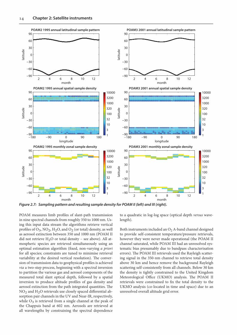
�e Polar Ozone and Aerosol Measurement II (POAM II) instrument was launched on-board the French SPOT-3 sat-ellite on 26 September 1993 into a 98.7° inclination, sun-synchronous orbit at an altitude of 833 km. �e instrument operated between October 1993 and November 1996 when the SPOT-3 satellite su�ered a malfunction and contact with the instrument was terminated. POAM III was launched on the  French SPOT-4 spacecra� on 24  March 1998 into an orbit identical to the one of SPOT-3. �e instrument began taking data on 22 April 1998 and operated until 5 Decem-ber 2005, when instrument failure terminated the mission. POAM III was functionally very similar to its predeces-sor, although it contained a number of design changes that improved sensitivity and accuracy. POAM II and III both used the solar occultation technique, measuring the ex-tinction of solar radiation in nine narrow-band channels from approximately 350 to 1060 nm and 353 to 1018 nm, respectively, to retrieve the vertical distribution of atmo-spheric O3, H2O, NO2, and aerosol extinction. Over their mission lifetimes, POAM II and III compiled datasets of ap-proximately 21,000 and more than 43,000 good occultation pro�les, respectively. POAM II and III made 14 measure-ments per day in each hemisphere, equally spaced in lon-gitude around a circle of approximately constant latitude. Satellite sunrise measurements were made in the Northern Hemisphere and sunsets in the Southern Hemisphere. Sun-rise measurements occur in a latitude band from 55-71°N while sunsets occur between 63-88°S.  �e latitude cover-age changes slowly with season and is exactly periodic from year to year. �e sampling patterns of POAM II and III are shown in Figure 2.7.

Vertical resolution of the POAM data products is approxi-mately 1 to 1.5 km, depending on the species. �e alti-tude range also varies by species and instrument version; for POAM II O3 (15-50 km), NO2 (20-40 km) and aero-sols (10-30 km), and for POAM III O3 (5-60 km), NO2 (20-40 km), H2O (5-45 km) and aerosols (5-25 km). Note that unlike POAM II, POAM III also provided a water va-pour product that was thoroughly validated against a va-riety of correlative satellite-, aircra�- and balloon-borne datasets. Due to uncertainties in the optical �lters for the di�erential water vapour channels, water vapour was never retrieved operationally from POAM II measurements.

A complete discussion of the POAM II instrument can be found in Glaccum et al. [1996]. �e Version 6 algorithms, error analysis and data characterisation are described by Lumpe et al. [1997]. A discussion of the POAM III instru-ment can be found in Lucke et al. [1999]. �e Version  4 algorithms, error analysis and data characterisation are de-scribed by Lumpe et al. [2002]. �e �nal public release da-tasets for POAM II (V6.0) and POAM III (V4) are available at the NASA Langley Atmospheric Sciences Data Center (http://www.eosweb.larc.nasa.gov) and are also distribut-ed by the Naval Research Laboratory via https://www.nrl.navy.mil/rsd/7220/poam-�p.

14 Chapter 2: Satellite instruments

POAM measures limb pro�les of slant-path transmission in nine spectral channels from roughly 350 to 1000 nm. Us-ing this input data stream the algorithms retrieve vertical pro�les of O3, NO2, H2O, and O2 (or total) density, as well as aerosol extinction between 350 and 1000 nm (POAM II did not retrieve H2O or total density – see above). All at-mospheric species are retrieved simultaneously using an optimal estimation algorithm (�xed, non-varying a priori for all species; constraints are tuned to minimise retrieval variability at the desired vertical resolution). �e conver-sion of transmission data to geophysical pro�les is achieved via a two-step process, beginning with a spectral inversion to partition the various gas and aerosol components of the measured total slant optical depth, followed by a spatial inversion to produce altitude pro�les of gas density and aerosol extinction from the path integrated quantities. �e NO2 and H2O retrievals use closely spaced di�erential ab-sorption pair channels in the UV and Near-IR, respectively, while O3 is retrieved from a single channel at the peak of the Chappuis band at 602 nm. Aerosols are retrieved at all wavelengths by constraining the spectral dependence

to a quadratic in log-log space (optical depth versus wave-length).

Both instruments included an O2 A-band channel designed to provide self-consistent temperature/pressure retrievals, however they were never made operational (the POAM II channel saturated, while POAM III had an unresolved sys-tematic bias presumably due to bandpass characterisation errors). �e POAM III retrievals used the Rayleigh scatter-ing signal in the 350-nm channel to retrieve total density above 30 km and hence remove the background Rayleigh scattering self-consistently from all channels. Below 30 km the density is tightly constrained to the United Kingdom Meteorological O�ce (UKMO) analysis. �e POAM II retrievals were constrained to �x the total density to the UKMO analysis (co-located in time and space) due to an unresolved overall altitude grid error.

Figure 2.7: Sampling pattern and resulting sample density for POAM II (left) and III (right).

POAM2 1995 annual latitudinal sample pattern

latit

ude

month2 4 6 8 10 12

−90

−60

−30

0

30

60

90

month

latit

ude

POAM2 1995 monthly zonal sample density

2 4 6 8 10 12−90

−60

−30

0

30

60

90

1

3

10

32

100

320

1000

3200

10000

longitude

latit

ude

POAM2 1995 annual spatial sample density

−180 −90 0 90 180−90

−60

−30

0

30

60

90

1

3

10

32

100

320

1000

3200

10000

POAM3 2001 annual latitudinal sample pattern

latit

ude

month2 4 6 8 10 12

−90

−60

−30

0

30

60

90

month

latit

ude

POAM3 2001 monthly zonal sample density

2 4 6 8 10 12−90

−60

−30

0

30

60

90

1

3

10

32

100

320

1000

3200

10000

longitude

latit

ude

POAM3 2001 annual spatial sample density

−180 −90 0 90 180−90

−60

−30

0

30

60

90

1

3

10

32

100

320

1000

3200

10000

15Chapter 2: Satellite instruments

2.2.6 OSIRIS on Odin

�e Odin satellite was launched on 20 February 2001 into a 600-km circular sun-synchronous near-terminator orbit with a 97.8° inclination [Murtagh et al., 2002]. Odin carries two instruments: the Optical Spectrograph and InfraRed Imager System (OSIRIS) [Llewellyn et al., 2004] and the Sub-Millimetre Radiometer (SMR; see Section 2.2.7) [Frisk et al., 2003]. �e instruments are co-aligned and scan the limb of the atmosphere through controlled nodding of the satellite over a tangent height range from 7 to 70 km in approximately 85 s (stratospheric mode, ~65 scans per orbit) or from 7-110 km in about 140  s (stratospheric-mesospheric mode, ~40  scans per orbit). Due to Odin’s orbit, the data from both instruments are generally limited to between 82°N and 82°S except for occasional short periods of o�-plane pointing at high latitudes during early polar spring. �e LSTs of the observations are close to 6pm and 6am for low and mid-latitudes during the ascending and descending nodes respectively, but sweep quickly

over local midnight and noon at the poles. Moreover, the equator crossing times are slowly dri�ing in LST during the Odin mission. A particularity of the Odin satellite is that observation times were initially equally shared between astronomical and atmospheric observation modes. �e astronomy mission ended in April 2007 and since then Odin has been entirely dedicated to atmospheric sciences.

OSIRIS is a grating spectrometer that measures limb-scattered sunlight spectra in the spectral range from 280  nm to 800 nm at a resolution of about 1 nm. �e scattered sunlight measurements are used to provide vertical pro�les of minor stratospheric constituents including O3, NO2, BrO and aerosol. Additional datasets exist, but only the o�cial products are mentioned here. Since OSIRIS observations are dependent on sunlight, the full latitude range is only covered around the equinoxes and hemispheric coverage is provided elsewhere. Examples of daily and annual sampling distributions are shown in Figure 2.8.

Figure 2.8: Sampling pattern and resulting sample density for Odin/OSIRIS for 2003 and 2009.

latit

ude

longitude

OSIRIS 2003 example daily sample pattern

−180 −90 0 90 180−90

−60

−30

0

30

60

90

Jan 1Jul 1

month

latit

ude

OSIRIS 2003 monthly zonal sample density

2 4 6 8 10 12−90

−60

−30

0

30

60

90

1

3

10

32

100

320

1000

3200

10000

longitude

latit

ude

OSIRIS 2003 annual spatial sample density

−180 −90 0 90 180−90

−60

−30

0

30

60

90

1

3

10

32

100

320

1000

3200

10000

latit

ude

longitude

OSIRIS 2009 example daily sample pattern

−180 −90 0 90 180−90

−60

−30

0

30

60

90

Jan 1Jul 1

month

latit

ude

OSIRIS 2009 monthly zonal sample density

2 4 6 8 10 12−90

−60

−30

0

30

60

90

1

3

10

32

100

320

1000

3200

10000

longitude

latit

ude

OSIRIS 2009 annual spatial sample density

−180 −90 0 90 180−90

−60

−30

0

30

60

90

1

3

10

32

100

320

1000

3200

10000

16 Chapter 2: Satellite instruments

�e NO2 (V3.0) product is retrieved using a combination of DOAS and the log-space optimal estimation method using wavelengths between 435 and 451 nm [Haley et al., 2004; Brohede et al., 2007a; Haley and Brohede 2007]. BrO (V5) is also retrieved with optimal estimation, but on zonally-averaged OSIRIS spectra, in the 346-377 nm range [ McLinden et al., 2010]. Ozone (V5) is retrieved with a mul-tiplicative algebraic reconstruction technique (MART) us-ing a range of doublet/triplets in the Hartley and Huggins bands [ Degenstein et al., 2009]. OSIRIS ozone pro�le mea-surements show agreement with coincident SAGE II oc-cultation measurements to within 2% from 18 to 53 km altitude over a large range of geo-locations and solar zenith angles. Stratospheric aerosol (V5) is also retrieved using a MART algorithm where the retrieval vector is designed to enhance the extra scattering, above the Rayleigh back-ground, due to sulphate aerosols [Bourassa et al., 2007]. For this vector a wavelength ratio of 750 nm to 470 nm is

used to characterise the e�ect of the Mie scattering signal. Hydrated sulphuric acid particle microphysics, including a size distribution for typical background aerosol, are as-sumed to calculate the scattering cross section and phase functions that are required to retrieve the aerosol extinc-tion. �e altitude range and resolution vary for each species and pro�le but are usually limited to the stratosphere and a maximum of ~2 km vertical resolution.

Inferred NOy, NOx and Bry data products are also com-piled using OSIRIS data, combined with photochemical box-model simulations for each individual pro�le [Brohede et al., 2008; McLinden et al., 2010], although Bry is not pre-sented in this report. Note that HNO3 observations from the Odin/SMR instrument are also used in the NOy prod-uct (NO2+NO+HNO3+ClONO2+2*N2O5). �e NOx data-set (NO2+NO) is not explicitly described in the literature but is compiled using box-model scaling factors, following

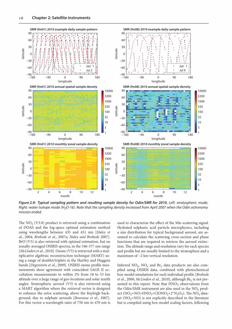
Figure 2.9: Typical sampling pattern and resulting sample density for Odin/SMR for 2010. Left: stratospheric mode; Right: water isotope mode (H2O-16). Note that the sampling density increased from April 2007 when the Odin astronomy mission ended.

latit

ude

longitude

SMR (fm01) 2010 example daily sample pattern

−180 −90 0 90 180−90

−60

−30

0

30

60

90

Jan 1Jul 2

month

latit

ude

SMR (fm01) 2010 monthly zonal sample density

2 4 6 8 10 12−90

−60

−30

0

30

60

90

1

3

10

32

100

320

1000

3200

10000

longitude

latit

ude

SMR (fm01) 2010 annual spatial sample density

−180 −90 0 90 180−90

−60

−30

0

30

60

90

1

3

10

32

100

320

1000

3200

10000

latit

ude

longitude

SMR (fm08) 2010 example daily sample pattern

−180 −90 0 90 180−90

−60

−30

0

30

60

90

Jan 1Jul 9

month

latit

ude

SMR (fm08) 2010 monthly zonal sample density

2 4 6 8 10 12−90

−60

−30

0

30

60

90

1

3

10

32

100

320

1000

3200

10000

longitude

latit

ude

SMR (fm08) 2010 annual spatial sample density

−180 −90 0 90 180−90

−60

−30

0

30

60

90

1

3

10

32

100

320

1000

3200

10000

17Chapter 2: Satellite instruments

the approach in Brohede et al. [2008]. Previous climatology studies and model inter-comparisons with OSIRIS data are described by Brohede et al. [2007b] for NO2, McLinden et al. [2010] for BrO/Bry and Brohede et al. [2008] for NOy. See the OSIRIS o�cial website for more information and data access: http://osirus.usask.ca/.

2.2.7 SMR on Odin

�e Sub-Millimetre Radiometer (SMR) on-board the Odin satellite (for launch and orbit details, see Section 2.2.6) uses four sub-millimetre and 1-millimetre wave radiometer to measure thermal emission from the atmospheric limb in the 486-581 GHz spectral range and around 119 GHz [Murtagh et al., 2002; Frisk et al., 2003]. �e signal is collected by a 1.1 m telescope and spectrally analysed by two auto-correlator spectrometers, each with 800 MHz bandwidth and 2 MHz e�ective resolution. Stratospheric mode observations of O3, ClO, N2O, HNO3, and H2O in the UTLS are performed using two bands around 501 and 544 GHz on every third observation day (on every other day since April 2007) [e.g., Urban et al., 2005a, 2006; Urban, 2008; Ekström et al., 2008]. Other regular observation modes are dedicated to the measurements of target species in the middle atmosphere such as water and ozone isotopologues around 490  GHz [Urban et al., 2007; Jones et al., 2009], mesospheric and lower thermospheric H2O at 557 GHz [Urban et al., 2007; Lossow et al., 2009; Orsolini et al., 2010], stratospheric and mesospheric CO, O3 and HO2 around 576 GHz [Dupuy et al., 2004; Jin et al., 2009; Baron et al., 2009], and H2O-17, O3, and NO in a band at 551 GHz [Urban et al., 2007]. For example, water isotope mode observations of H2O16 were performed on 1 day per week until 2007 (10 days per month since April 2007). �e sampling pattern and resulting measurement density from SMR for the stratospheric mode and the water isotope mode can be seen in Figure 2.9.

Vertical pro�les (Level-2 data) are retrieved from the calibrated spectral measurements of the limb scans (Level-1b data) by inverting the radiative transfer equation for a non-scattering atmosphere. Employed retrieval techniques for Odin/SMR Level-2 processing are based on the optimal estimation method (except for upper tropospheric humidity and ice) [Urban et al., 2004; Buehler et al., 2005; Eriksson et al., 2005]. �e altitude range and resolution varies for each species depending on the signal-to-noise ratio and frequency band employed. Currently recommended data versions are V2.0 for the 544 GHz band and V2.1 for all other modes.

Climatologies of several species (N2O, HNO3, NO2, NOy, CO, ClO, O3), derived from Odin observations since 2001 and compiled in terms of altitude or equivalent latitude versus pressure, altitude, or potential temperature, are avail-able from the Odin/SMR website (http://odin.rss.chalmers. se). For information on the climatologies of HNO3, NO2, and derived NOy the reader is referred to Urban et al. [2009], Brohede et al. [2007a] and Brohede et al. [2008].

2.2.8 GOMOS on Envisat

GOMOS (Global Ozone Monitoring by Occultation of Stars) was a stellar occultation instrument on-board the European Space Agency’s Environmental satellite, Envisat [Bertaux et al., 2010; http://envisat.esa.int/handbooks/gomos/]. Envisat was launched into its sun-synchronous polar orbit of 98.55° inclination at about 800 km altitude on 1 March 2002. Contact to the satellite was lost on 8 April 2012. Its equator crossing time was 10am. For every occultation GOMOS �rst measured a star's reference spectrum when the star was seen above the atmosphere. �is reference spectrum and the spectra measured through the atmosphere were used to calculate the horizontal transmission spectra through the atmosphere. Transmissions are the basis for spectral and vertical retrieval of species pro�les. GOMOS performed 100-200 night occultations per day. �e measurement coverage of night occultations was global, except in the

Figure 2.10: Sampling pattern and resulting sample den-sity for GOMOS.

latit

ude

longitude

GOMOS 2003 example daily sample pattern

−180 −90 0 90 180−90

−60

−30

0

30

60

Jan 3Jul 1 9

month

latit

ude

GOMOS 2003 monthly zonal sample density

2 4 6 8 10 12−90

−60

−30

0

30

60

90

1

3

10

32

100

320

1000

3200

10000

longitude

latit

ude

GOMOS 2003 annual spatial sample density

−180 −90 0 90 180−90

−60

−30

0

30

60

90

1

3

10

32

100

320

1000

3200

10000

18 Chapter 2: Satellite instruments

summer-time polar regions. Daytime occultations were also measured, but they are not used in the present work due their lower quality. Measurements start at 150 km and extend down to 5 km in cloudless conditions. �e altitude-sampling resolution is 0.5-1.7 km and depends on the azimuth of the LOS with respect to the orbital plane. �e nominal vertical resolution of the retrieved ozone pro�les is 2 km below 30 km, 2-3 km between 30-40 km and 3 km above 40 km, and for other species about 4 km (see also Section 3.1.3.8). �e instrument optical design was based on a 30-cm telescope that simultaneously fed UV-VIS and IR spectrometers, two fast photometers and two redundant star trackers. Spectra were recorded by CCD detectors. �e UV-VIS spectrometer spectral range were 250-690 nm with 0.3 nm sampling and 0.9 nm resolution. �e constituents retrieved are O3, NO2, NO3, and aerosol. �e IR spectrometer channels are 750-776  nm and 916-956 nm with 0.06 nm sampling and 0.1 nm resolution. IR data are used to retrieve O2 and H2O. Two fast (1 kHz) photometers at blue and red wavelengths were used to make the scintillation correction for the spectrometer data, retrieve high-resolution temperature pro�le and probe stratospheric turbulence.

�e self-calibrating measurement principle with good ver-tical resolution and accurate vertical geo-location made GOMOS a good candidate to produce long time series and climatologies (see Hauchecorne et al. [2005], Kyrölä et al. [2006, 2010a, 2010b], Vanhellemont [2010]). However, dif-�culties with the pointing system in 2003, 2005 and 2009 have le� some gaps in the data coverage. Noise levels of the CCDs increased steadily from the launch date, and this has led to a decrease in the quality of data over time. �e sampling pattern and resulting measurement density from GOMOS can be seen in Figure 2.10.

�e climatologies are constructed using GOMOS data from ESA processing Version IPF 5. �e retrieval scheme is discussed in Kyrölä et al. [2010b]. �e GOMOS constitu-ent pro�le retrieval starts from the horizontal transmission spectra. Occultations are processed one at a time. �e data processing is split into Level 1b and Level 2 stages. In Level 1b, dark charge removal and other instrumental correc-tions are performed and �nally transmission spectra are constructed. Geo-location is determined starting from the satellite location and from the known direction of the star, and performing ray-tracing calculations with the atmo-sphere assumed to be the one given by the ECMWF data below 1 hPa and the MSIS90 climatology in the upper at-mosphere. In Level 2 processing, the transmission spectra are �rst corrected for dilution caused by refraction and for modulations by scintillations. �e fast photometer data are used in the scintillation correction. In case of o�-orbital-plane occultations, the correction is not able to remove the scintillation modulation arising from isotropic turbulence in the LOS. �e ozone retrieval, however, is only weakly sen-sitive to modulations by scintillations [So�eva et al., 2010]. Ozone as well as NO2, NO3, and aerosols are retrieved from the UV/VIS range 250-675 nm. �e Rayleigh extinc-tion is removed using the ECMWF+MSIS90 data. �e UV/

VIS retrieval is divided into two consecutive stages. In the spectral inversion the model transmission function is �tted by a non-linear Levenberg-Marquardt method to the trans-missions. Because of perturbations caused by uncorrected isotropic scintillations, NO2 and NO3 retrievals are based on sub-iteration using the di�erential cross section method [see Hauchecorne et al., 2005].

A�er spectral inversion the vertical inversion is performed using so-called onion-peeling method. �e inversion is constrained using the target resolution Tikhonov method [So�eva et al., 2004]. For ozone the target vertical resolu-tion is 2 km below 30 km and 3 km above 40 km. For other constituents the target vertical resolution is 4 km. An itera-tion loop over spectral and vertical inversion is performed in order to take into account the temperature dependence of the cross sections. �e retrieval errors for constituent pro�les depend on the brightness of the star measured. For ozone, the error depends also on the spectral type of the star. Data quality and error estimates of GOMOS are dis-cussed in detail in Tamminen et al. [2010].

2.2.9 MIPAS on Envisat

�e Michelson Interferometer for Passive Atmospheric Sounding (MIPAS) was a mid-infrared Fourier trans-form limb emission spectrometer designed and operated for measurement of atmospheric trace species from space [Fischer et al., 2008]. It was part of the instrumentation of Envisat (for launch and orbit details, see Section 2.2.8). MIPAS passed the equator in a southerly direction at 10am local time 14.3 times a day, observing the atmosphere dur-ing day and night with global coverage from pole to pole. �e instrument’s �eld of view was 30 km in the horizontal and approximately 3 km in the vertical direction. MIPAS covered the 4.3-15 µm region in �ve spectral bands: band A (685-970 cm−1), AB (1020-1170 cm−1), B (1215-1500 cm−1), C (1570-1750 cm−1), and D (1820-2410 cm−1).

MIPAS operated during July 2002 – March 2004 at full spectral resolution of 0.035 cm−1 (unapodised) in terms of full width at half maximum. During this period, MIPAS recorded a rear-viewing limb sequence of 17 spectra each 90 seconds, corresponding to an along track sampling of approximately 500 km and providing about 1000 vertical pro�les per day in its standard observation mode. Tangent heights covered then the altitude range from 68 down to 6 km with tangent altitudes at 68, 60, 52, 47, and then at 3 km steps from 42 to 6 km.

Due to problems with the interferometer-mirror-slide system, MIPAS performed few operations from April–December 2004. In January 2005 regular observations resumed, but with a reduced duty cycle and a reduced spectral resolution of 0.0625 cm−1. �ese new measurements have the advantage that more spectra could be measured during the same time interval compared to the former “high”-spectral resolution observations. Tangent heights covered the range from 70 down to 6 km with tangent

19Chapter 2: Satellite instruments

altitudes at 70, 66, 62, 58, 54, 50, 46, 43, 40, 37, 34, 31, 29, 27, 25, 23, and then at 1.5 km steps from 21 to 6 km. Due to this modi�ed measurement scenario the number of pro�les increased by about 20%.

Trace gas pro�les included in this climatology have been retrieved from calibrated geo-located limb emission spec-tra with the MIPAS Level 2 research processor developed and operated by the Institute of Meteorology and Climate Research (IMK) in Karlsruhe together with the Instituto de Astrofísica de Andalucía (IAA) in Granada. �e general retrieval strategy, which is a constrained multi-parameter non-linear least squares �tting of measured and modelled spectra, is described in detail in von Clarmann et al. [2003c]. Its extension to retrievals under consideration of non-LTE (CO, NO, and NO2) is described in Funke et al. [2001]. A�er wavenumber-recalibration, target quantities are re-trieved sequentially, starting with temperature and LOS elevation (from CO2 emissions around 15 µm), followed by the atmospheric main IR emitters H2O, O3, CH4 and

N2O. A�erwards all other species are retrieved under con-sideration of the results of the preceding retrievals. Instead of the commonly used optimal estimation scheme, a Tik-honov-type �rst order regularisation is used [Steck and von Clarmann, 2001] because it does not constrain the column information but only how this information is distributed over altitude and, thus, does not push the mixing ratios to-wards a priori information. �e strength of the regularisa-tion is altitude dependent, with the aim of �nding the best trade-o� between the vertical resolution and the precision of the retrieved parameters. While trace gas abundances are retrieved in terms of VMR for most species, for some spe-cies (H2O, NO2, NO, CO), ln(VMR) is retrieved instead in order to better account for their pronounced temporal and spatial variability and reduce their dynamical range. Fur-ther, some target quantities (temperature and the trace gas-es NO, NO2, and CO) are characterised by a pronounced spatial inhomogeneity, particularly close to transport bar-riers. In these cases, horizontal gradient pro�les are taken into account within the retrieval [Kiefer, 2010]. In addition,

Figure 2.11: Sampling pattern and resulting sample density for MIPAS. Left panels show results for the full (high)-spectral resolution mode from 2002-2004, right panels for the reduced (low)-spectral resolution mode from 2005-ongoing.

latit

ude

longitude

MIPAS high−res example daily sample pattern

−180 −90 0 90 180−90

−60

−30

0

30

60

90

Jan 1Jan 2

month

latit

ude

MIPAS high−res monthly zonal sample density

2 4 6 8 10 12−90

−60

−30

0

30

60

90

1

3

10

32

100

320

1000

3200

10000

longitude

latit

ude

MIPAS high−res annual spatial sample density

−180 −90 0 90 180−90

−60

−30

0

30

60

90

1

3

10

32

100

320

1000

3200

10000

latit

ude

longitude

MIPAS low−res example daily sample pattern

−180 −90 0 90 180−90

−60

−30

0

30

60

90

Jan 1Jan 2

month

latit

ude

MIPAS low−res monthly zonal sample density

2 4 6 8 10 12−90

−60

−30

0

30

60

90

1

3

10

32

100

320

1000

3200

10000

longitude

latit

ude

MIPAS low−res annual spatial sample density

−180 −90 0 90 180−90

−60

−30

0

30

60

90

1

3

10

32

100

320

1000

3200

10000

20 Chapter 2: Satellite instruments

a radiance o�set and a continuum-like optical depth pro�le are �tted jointly for each microwindow in order to com-pensate for calibration errors and atmospheric contribu-tions of weak wavenumber dependence not reproduced by the radiative transfer forward model [von Clarmann et al., 2003c]. �e MIPAS-IMK/IAA research data product, along with related diagnostics, is available to registered users via http://www.imk-asf.kit.edu/english/308.php. �e sam-pling patterns and resulting measurement densities from MIPAS high and reduced spectral resolution measurement modes can be seen in Figure 2.11.

2.2.10 SCIAMACHY on Envisat

�e Scanning Imaging Absorption spectroMeter for At-mospheric CHartographY (SCIAMACHY) [Burrows at al., 1995, Bovensmann et al., 1999] was a payload on Envisat launched in March 2002 (for launch and orbit details, see Section 2.2.8). SCIAMACHY was one of the new-generation

of space-borne instruments capable of performing spec-trally-resolved measurements in several di�erent modes: alternate nadir and limb observations of the solar radia-tion scattered by the atmosphere or re�ected by the Earth’s surface; and observations of the light transmitted through the atmosphere during solar or lunar occultation when feasible. �e SCIAMACHY instrument was a passive im-aging spectrometer comprised of eight spectral channels covering a wide spectral range from 214 to 2386 nm. Each spectral channel comprised a grating spectrometer, having a 1024-element diode array as a detector. Depending on the spectral channel the spectral sampling ranged from 0.11 to 0.74 nm and the spectral resolution from 0.22 to 1.48 nm.

�is study uses SCIAMACHY measurements from scat-tered solar light in the limb-viewing geometry. In this ge-ometry, the atmosphere was observed tangentially to the Earth’s surface starting at about 4.5 km below the horizon (~1.5 km below the horizon since January 2011), i.e., when the Earth’s surface was still within the �eld-of-view of the instrument, and then scanning vertically up to the top of the neutral atmosphere (about 100 km tangent height). At each tangent height a horizontal scan of 1.5 s duration was performed followed by an elevation step of about 3.3 km. No measurements were performed during the vertical step. �is results in a vertical sampling of 3.3 km. �e vertical in-stantaneous �eld-of-view of the SCIAMACHY instrument was about 2.6 km at the tangent point. Although the hori-zontal instantaneous �eld-of-view of the instrument was about 110 km at the tangent point, the horizontal resolution was mainly determined by the integration time during the horizontal scan, reaching typically about 240 km. �e entire distance at the tangent point covered by the horizontal scan was about 960 km. �e along-track horizontal resolution was estimated to be about 400 km. In the nominal mode, about 100 measurements per orbit with 14 complete orbits per day were performed. Global coverage was achieved af-ter six days. �e sampling pattern and resulting data den-sity for SCIAMACHY limb observations can be seen in Figure  2.12. �e sampling pattern shown in Figure 2.12 refers to standard retrievals with measurements at SZAs of up to 89°, resulting in a maximum latitude coverage of 65° in the winter hemisphere. �is applies to all SCIAMACHY climatologies used in this study except for water vapour, for which only measurements at SZAs smaller than 85° are processed, resulting in a reduced latitude coverage of 55°. �e gap in the sampling seen in the Southern Hemisphere is due to the South Atlantic anomaly. In this area the instru-ment electronics were exposed to an increased �ux of ener-getic particles, which disturbed the measured signal result-ing in a signi�cant retrieval bias. �is makes it necessary to reject the a�ected data when creating the climatologies (see Section 3.1.3.10 for details).

Similar to other limb scattering instruments, the pointing uncertainty is a major error source. Currently, the accuracy of the pointing for the whole limb scan is estimated to be about 200 m. �e relative pointing error between di�er-ent tangent heights is negligible. �e measurements at the lower tangent heights are a�ected by clouds; no retrievals

Figure 2.12: Sampling pattern and resulting sample density for SCIAMACHY.

latit

ude

longitude

SCIAMACHY 2010 example daily sample pattern

−180 −90 0 90 180−90

−60

−30

0

30

60

90

Jan 1Jan 2

month

latit

ude

SCIAMACHY 2010 monthly zonal sample density

2 4 6 8 10 12−90

−60

−30

0

30

60

90

1

3

10

32

100

320

1000

3200

10000

longitude

latit

ude

SCIAMACHY 2010 annual spatial sample density

−180 −90 0 90 180−90

−60

−30

0

30

60

90

1

3

10

32

100

320

1000

3200

10000

21Chapter 2: Satellite instruments

can be done in the presence of a cloud in the instrument �eld-of-view.

More general information on the SCIAMACHY instru-ment can be found at http://envisat.esa.int/instruments/sciamachy/ and http://www.iup.physik.uni-bremen.de/sciamachy/.

Vertical pro�les of atmospheric species and aerosol extinc-tion coe�cients included in this climatology are retrieved from SCIAMACHY limb measurements using the scienti�c processor developed and operated by the Institute of the Environmental Physics (IUP) at the University of Bremen. Depending on the species, several spectral sub-windows in UV, visible, or near-infrared spectral ranges are used. Re-trievals of O3 and aerosol extinction coe�cients exploit ra-diance pro�les averaged over several nanometer wide spec-tral windows, whereas NO2, BrO, and H2O algorithms gain information from the di�erential structure of the trace gas absorption bands (DOAS technique). All retrievals except for H2O use the reference tangent height normalisation technique to reduce the in�uence of the solar Fraunhofer lines, instrument calibration errors, and radiation scattered in the lower troposphere or re�ected from the underlying surface. �e retrieval relies on the optimal estimation type technique including an additional smoothing constraint (�rst order Tikhonov term). �e non-linearity of the in-verse problem is accounted for by employing the Gauss-Newton iterative scheme.

For most species, the retrieval is done for number densities while for H2O the logarithms of the number densities are retrieved. Details on the retrieval algorithms and validation results for di�erent species can be found in Rozanov et al. [2005], Ernst et al. [2009], Sonkaev et al. [2009], Bauer et al. [2012], Mieruch et al. [2012], Rozanov et al. [2011a; 2011b]. �e SCIAMACHY scienti�c products retrieved by IUP Bremen are available to registered users via http://www.iup.physik.uni-bremen.de/scia-arc. Except for the aerosol extinction coe�cients, the results are provided along with the averaging kernels, retrieval precision, and cloud �ags.

2.2.11 ACE-FTS on SCISAT-1

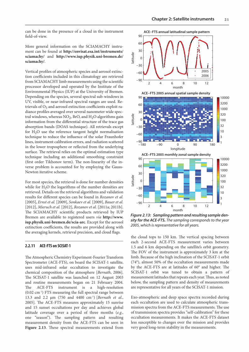
�e Atmospheric Chemistry Experiment-Fourier Transform Spectrometer (ACE-FTS), on board the SCISAT-1 satellite, uses mid-infrared solar occultation to investigate the chemical composition of the atmosphere [Bernath, 2006]. �e SCISAT-1 satellite was launched on 12 August  2003 and routine measurements began on 21 February  2004. �e ACE-FTS instrument is a high-resolution (0.02 cm-1) FTS measuring the full spectral range between 13.3 and 2.2 μm (750 and 4400 cm-1) [Bernath et al., 2005]. �e ACE-FTS measures approximately 15  sunrise and 15 sunset occultations per day and achieves global latitude coverage over a period of three months (e.g., one “season”). �e sampling pattern and resulting measurement density from the ACE-FTS can be seen in Figure 2.13. �ese spectral measurements extend from

the cloud tops to 150 km. �e vertical spacing between each 2-second ACE-FTS measurement varies between 1.5 and 6 km depending on the satellite’s orbit geometry. �e FOV of the instrument is approximately 3 km at the limb. Because of the high inclination of the SCISAT-1 orbit (74°), almost 50% of the occultation measurements made by the ACE-FTS are at latitudes of 60° and higher. �e SCISAT-1 orbit was tuned to obtain a pattern of measurement latitudes that repeats each year. �us, as noted below, the sampling pattern and density of measurements are representative for all years of the SCISAT-1 mission.

Exo-atmospheric and deep space spectra recorded during each occultation are used to calculate atmospheric trans-mission spectra from the ACE-FTS measurements. �e use of transmission spectra provides “self-calibration” for these occultation measurements. It makes the ACE-FTS dataset less susceptible to changes over the mission and provides very good long-term stability in the measurements.

Figure 2.13: Sampling pattern and resulting sample den-sity for the ACE-FTS. The sampling corresponds to the year 2005, which is representative for all years.

month

latit

ude

ACE−FTS annual latitudinal sample pattern

2 4 6 8 10 12−90

−60

−30

0

30

60

90

20052006

month

latit

ude

ACE−FTS 2005 monthly zonal sample density

2 4 6 8 10 12−90

−60

−30

0

30

60

90

1

3

10

32

100

320

1000

3200

10000

longitude

latit

ude

ACE−FTS 2005 annual spatial sample density

−180 −90 0 90 180−90

−60

−30

0

30

60

90

1

3

10

32

100

320

1000

3200

10000

22 Chapter 2: Satellite instruments

Level 2 constituent pro�les are retrieved from the ACE-FTS transmission spectra in VMR using an unconstrained non-linear least squares global �tting approach [Boone et al., 2005, and references therein]. In the �rst step, CO2 lines in the spectra are used to determine the pressure and temperature as a function of altitude. �e micro-windows used for the retrieval cover the following wavenumber ranges: 932–937, 1890–1976, 2042–2073, 2277–2393, 2408–2448, 3301–3380, and 3570–3740 cm-1. Temperature and pressure pro�les are retrieved from the ACE-FTS spectra between 12 and 120 km. Below 12 km, meteorological results from the Canadian Meteorological Centre operational weather analysis and forecast system are used. Above 120 km, output from the Naval Research Laboratories MSISE-00 so�ware is employed. �e resulting temperature and pressure pro�les are used to retrieve VMR pro�les of over 30 trace gas species from sets of micro-windows chosen to contain spectral features speci�c to each of the target molecules. �e spectroscopic parameters used for these calculations are from the HITRAN 2004 linelist [Rothman et al., 2005]. �e retrieval algorithm uses �rst guess pro�les taken from the four ATMOS missions on-board the Space Shuttle. However, the retrievals are not constrained by these �rst guess pro�les. Currently, there is no error budget available for the ACE-FTS products. For each measurement, there is an associated �tting uncertainty provided. �is one-sigma �tting uncertainty is the square root of the diagonal element of the covariance matrix obtained in the retrieval process [Boone et al., 2005]. A document describing the microwindows used for the ACE-FTS retrievals is available from http://www.ace.uwaterloo.ca [ACE Report ACE-SOC-0020, Microwindow List for ACE-FTS retrievals – Version 2.2 + updates, Dec. 2006].

For the SPARC Data Initiative, the ACE-FTS Version 2.2 data products are used including updates for O3 and N2O5. �e validation results for these species and parametres are included in a special issue of Atmos. Chem. Phys. (http://www.atmos-chem-phys.org/special_issue114.html). In addition, two climatologies have been created for the 2004-2009 period using the Version 2.2 (plus updates) dataset: a climatology for O3, H2O, CH4, N2O, CO, NO, NO2, N2O5, HNO3, HCl, ClONO2, CCl3F, CCl2F2, and HF [Jones et al., 2012] and an NOy climatology derived from the ACE-FTS NO, NO2, HNO3, HNO4, N2O5 and ClONO2 products [Jones et al., 2011]. Both are �ve-year zonal mean clima-tologies provided on a monthly and three-month basis. �e Level 2 ACE-FTS data products are stored by occultation in ASCII format (main isotopologues and minor isotopo-logues are in separate �les for each occultation). Further information about ACE-FTS and the ACE mission, includ-ing the Level 2 Version 2.2 data products, can be found at: http://www.ace.uwaterloo.ca/.

2.2.12 ACE-MAESTRO on SCISAT-1

�e Measurement of Aerosol Extinction in the Stratosphere and Troposphere Retrieved by Occultation (MAESTRO) is a dual UV/VIS/Near-IR spectrophotometer that is part

of the Atmospheric Chemistry Experiment (ACE) mis-sion on-board the SCISAT-1 satellite [McElroy et al., 2007]. ACE-MAESTRO was designed to extend the ACE wave-length coverage to the 280-1030 nm spectral region using two spectrometers with overlapping coverage (280-550 nm, 500-1030 nm) to reduce stray light. Currently, it makes mea-surements of solar radiation between 450-1030 nm during each sunrise and sunset with a spectral resolution of 1-2 nm (depending on spectral region). �e two ACE instruments take simultaneous measurements of the same air mass us-ing a common sun-tracking mirror that is located within the ACE-FTS. During each occultation (sunrise or sunset measurement), approximately 60 spectra are measured by ACE-MAESTRO between the cloud tops and 100 km. �e vertical spacing of these measurements varies from 300 m to 2 km at altitudes below 50 km and the spacing increases to every 5 km for altitudes above 50 km. �e FOV of the instrument is approximately 1 km at the limb.

As noted in Section 2.2.11, the SCISAT-1 satellite was launched on 12 August 2003 and began routine measure-ments on 21 February 2004. �e sampling pattern and resulting measurement density from ACE-MAESTRO is essentially identical to that of ACE-FTS (as shown in Figure 2.13). As can be seen in Figure 2.13, ACE-MAESTRO achieves global latitude coverage in its measurements over a period of three months.

Level 2 pro�les of O3, NO2, and optical depth are retrieved from the ACE-MAESTRO measurements as a function of altitude using a di�erential optical method combined with an interactive Chahine relaxation inversion algorithm [McElroy et al., 2007, and references therein]. In the �rst step, the raw data are converted to wavelength-calibrated spectra, corrected for stray light, dark current and other instrument parameters. �en, a non-linear least-squares spectral �tting routine is used to analyse the corrected spectra. �ese are used to calculate slant-path column den-sities for each spectrum and, from these, vertical pro�les of O3 and NO2 VMRs are derived by adjusting an initial guess pro�le from a high-vertical-resolution model simula-tion. Pressure and temperature pro�les used in the ACE-MAESTRO retrievals are obtained from the corresponding ACE-FTS occultation measurement and are used to �x the tangent heights for the ACE-MAESTRO retrievals. �e re-trieval algorithm does not require any a priori information or other constraints [McElroy et al., 2007]. No error budget has been produced for the ACE-MAESTRO data products. For each measurement, there is an associated error pro-vided. �is is essentially the random error of the measure-ment and is produced by propagating the instrument noise through the spectral �tting and pro�le retrieval codes.

For this project, the ACE-MAESTRO Version 1.2 O3 data products are used, which are available from: http://www.ace.uwaterloo.ca. �e Level 2 ACE-MAESTRO data prod-ucts for each species/parameter are stored individually by occultation in ASCII format. �e validation of the ACE-MAESTRO ozone product was described by Dupuy et al. [2009] and is part of the special issue of Atmospheric

23Chapter 2: Satellite instruments

Chemistry and Physics (described above: http://www. atmos-chem-phys.org/special_issue114.html).

2.2.13 HIRDLS on Aura

�e High Resolution Dynamics Limb Sounder (HIRDLS) instrument is a 21-channel limb-scanning infrared radiometer, designed to scan from the upper troposphere into the mesosphere and provide data with 1-km vertical resolution. HIRDLS was launched on the Aura satellite into a polar orbit on July 15, 2004 (see Section 2.2.15). �e original description of the experiment is by Gille and Barnett [1992]. Its channels cover the wavelength range from 6.12 to 17.76  μm, or 563 -1634 cm-1, in order to measure emission features from 11 trace gases and from aerosols. Four channels measure emission by CO2, from which temperature is recovered as a function of pressure. �ree channels are dedicated to the retrieval of O3, two to H2O, and one each to CH4, N2O, NO2, N2O5, HNO3, ClONO2,

CFC-11 and CFC-12, with others for measurement of aerosols at four wavelengths. �e large number of channels allows several to be dedicated to obtaining measurements in weaker parts of the bands, allowing sounding of the upper troposphere.

Unfortunately, HIRDLS was damaged during launch such that most of the aperture was covered. �e blocking ma-terial is believed to be a thin �lm of plastic that became dislodged during launch and settled in the optical train, blocking 80-95% of the beams leading to the 21 detectors. In addition to blocking the aperture areas, this material gives o� radiance signals that vary with scan angle and time on many scales. Gille et al. [2008] give a post-launch de-scription of HIRDLS. Data coverage is from 63°S to 80°N, with pro�les spaced every 100 km along the scan track, as shown in Figure 2.14. Because three of the retrieved spe-cies have diurnal variations, it is also important to know the local time of the retrievals on the ascending (northward) and descending portions of the orbit. Gille et al. [2008] also describes the initial corrections that resulted in Version 3 (V3) data. While details have changed, the procedure is the same for the V6 data discussed here.

Vertical coverage varies for each species, but the 1 km vertical resolution has been preserved. Persistent e�ort has resulted in successive improvements, leading to the release of the V6 data relevant to this report. �ey include temperature, O3, HNO3, CFC-11, CFC-12, and zonal means of day (1500 UT) and night (0 UT) NO2, and night N2O5. All products for a single day are in a single �le, on a grid of 24 pressure levels per decade of pressure, uniformly distributed in log pressure. More detailed characteristics of these data are included in the Data Description and Quality Document, Version 6, available from http://archive-eos.acom.ucar.edu/hirdls/, http://disc.sci.gsfc.nasa.gov/data-holdings, or http://badc.nerc.ac.uk/browse/badc/hirdls.

HIRDLS data are calibrated, corrected and retrieved in two major processors. In the �rst, the L1 processor, the conver-sion from raw counts to corrected radiances takes place, and the scans are geo-located. Subsequently they are cor-rected for the e�ects of the blocking material. �e �rst cor-rection is the removal of the small amplitude oscillations at ~1.8 Hz, which are initiated when the scan mirror contacts the plastic �lm during a scan. Next, the signal emitted by the �lm is removed, based on measurements made when Aura is pitched so that the complete HIRDLS scan is above the atmosphere, and only the �lm is viewed. Finally, the sig-nal is corrected for the reduced e�ective aperture. Recent e�orts have been made to model more closely the signal from the �lm, especially its change over the 3-year mission. A�er these corrections are made, the input radiances are on a nearly unifom elevation angle scale with a spacing that corresponds to ~200 m at the limb. �ey are then �ltered to remove noise at spatial frequencies too high to be seen by HIRDLS, then splined onto an altitude grid with 1 km spac-ing. Channel 6 near 830 cm-1 is in the most transparent por-tion of the spectrum; it is used for the detection of clouds and aerosols. �e altitude at which channel 6 radiances

Figure 2.14: Sampling pattern and resulting sample den-sity for HIRDLS.

latit

ude

longitude

HIRDLS 2006 example daily sample pattern

−180 −90 0 90 180−90

−60

−30

0

30

60

90

Jan 1Jan 2

month

latit

ude

HIRDLS 2006 monthly zonal sample density

2 4 6 8 10 12−90

−60

−30

0

30

60

90

1

3

10

32

100

320

1000

3200

10000

longitude

latit

ude

HIRDLS 2006 annual spatial sample density

−180 −90 0 90 180−90

−60

−30

0

30

60

90

1

3

10

32

100

320

1000

3200

10000

24 Chapter 2: Satellite instruments

suddenly increase is tagged as the cloud top, but it is veri-�ed and possibly adjusted with data from channel 12. �ese are input to the second step, the L2 retrieval processor.

�e retrieval algorithm is based on optimal estimation theo-ry [Rodgers, 2000], using a modi�ed Levenberg-Marquardt approach for the iterative solution. �e application for HIRDLS is described in detail in Khosravi et al. [2009]. �e L2 step accepts the conditioned radiance data from the L2CLD, where cloud top heights are determined, and per-forms the retrievals through a series of iterations. �is code is designed to be �exible in handling combinations of radi-ance channels to retrieve the HIRDLS target species in a user-de�ned sequence. One of the major features is the use of ancillary data from the Goddard Earth Observing Sys-tem Model (GEOS-5), produced by NASA’s Global Mod-eling and Assimilation O�ce (GMAO) to determine tem-perature gradients along the LOS, which are incorporated to yield improved retrievals. �is processor is described in detail in the L1-2 Algorithm �eoretical Basis Document

(ATBD) available on the web at http://archive-eos.acom.ucar.edu/hirdls/data/products/HIRDLS-DQD_V6-1.pdf. GEOS-5 Version 5.01 data were used through January 2, 2008, a�er which Version 5.1 data were used.

2.2.14 MLS on Aura

Aura-MLS is a Microwave Limb Sounder (MLS) instru-ment, which is part of the Earth Observing System (EOS) and launched on the Aura satellite on 15 July 2004 (for orbit details, see Section 2.2.15). Aura-MLS, like its predecessor version on the UARS (see Section 2.2.4), measures micro-wave thermal emission day and night, simultaneously from several spectral regions, using an antenna that scans the Earth’s atmospheric limb, in this case every 24.7 s.

Aura-MLS measures thermal emission from the limb in �ve broad spectral regions between 118 GHz and 2.5 THz. Aura-MLS views the atmosphere ahead of the Aura satel-lite, which is in a sun-synchronous near-polar orbit, with a ~1:45pm equatorial crossing time (ascending node). �e MLS vertical scans are synchronised to the Aura orbit, leading to retrieved pro�les at the same latitude every or-bit, with a spacing of 1.5° great circle angle (about 165 km) along the sub-orbital track; the horizontal (along-track) resolution is limited by the smearing of sensitivity near the tangent point, including the impact of retrieval smoothing constraints, but typically ranges from 200 to 500 km in the stratosphere. �e 240 limb scans per orbit provide almost 3500 pro�les (per species) every day, from about 82°S to 82°N. �e sampling pattern and resulting measurement density from Aura-MLS can be seen in Figure 2.15. �e vertical retrievals are typically on a pressure grid with six levels (pressure surfaces) per decade change in pressure in the stratosphere and lower mesosphere; the main Version 3.3 exception relevant for (and used in) this report is the H2O product, which is retrieved on a vertical grid that is twice as �ne as that for most other species.

�e Aura-MLS retrievals use the “optimal estimation” method [Rodgers, 1976; 2000]. �is involves the nonlinear weighted least squares optimisation of a cost function de-scribing the �t to observed radiance signals, including the use of a priori constraints for regularisation. Uncertainty estimates are provided as a result of the inversion process, based on input radiance uncertainties and a priori pro�le uncertainties. Gauss-Newton iteration is used, with a sec-ond order Tikhonov constraint [Tikhonov, 1963]; this con-straint is applied to the pro�le second derivatives (vertically and horizontally). Speci�c retrieval aspects include adap-tation to a two-dimensional system, using the LOS mea-surements from several scans to derive information about several pro�les [see Livesey and Read, 2000]. �e various species are retrieved from overlapping “chunks” of observa-tions, typically consisting of a 15° span of great circle angle (about ten vertical scans). Several retrieval “phases” are per-formed in sequence, each using a di�erent set of measured radiances; some phases retrieve temperature and pressure, and some include this information from an earlier phase. In

Figure 2.15: Sampling pattern and resulting sample density for Aura-MLS.

latit

ude

longitude

AURA MLS 2005 example daily sample pattern

−180 −90 0 90 180−90

−60

−30

0

30

60

90

Jan 1Jan 2

month

latit

ude

AURA MLS 2005 monthly zonal sample density

2 4 6 8 10 12−90

−60

−30

0

30

60

90

1

3

10

32

100

320

1000

3200

10000

longitude

latit

ude

AURA MLS 2005 annual spatial sample density

−180 −90 0 90 180−90

−60

−30

0

30

60

90

1

3

10

32

100

320

1000

3200

10000

25Chapter 2: Satellite instruments

the MLS retrieval system, the state vector represents verti-cal pro�les of mixing ratios in a piecewise-linear manner. �e only exception is water vapour, where the representa-tion is piecewise-linear in the logarithm of the VMR, nev-ertheless the retrieved quantity is VMR.

�e Aura-MLS Level 2 data �les include various screening �ags to provide users with information about instrument and retrieval status (and also about quality of �t and retriev-al convergence) based on various criteria described in the species-speci�c V2.2 validation papers. �e updated V3.3 retrievals used to generate the SPARC Data Initiative cli-matologies for this report (except for ozone, for which V2.2 is recommended overall because of vertical oscillations that exist primarily in V3.3 in the UTLS at low latitudes) follow generally the same (V2.2) �agging/screening methodolo-gies and recommendations for data usage, albeit with some changes in the screening �ag threshold values. Also, the V3.3 data for CO and HNO3 (used here) are more sensitive to cloud e�ects than previous versions, as a result of chang-es in the retrieval approach and the vertical range used in the UT. �e resulting data screening methods include the removal of negative outliers (spikes of a certain size), as described in the V3.3 Aura MLS Data Quality documen-tation [Livesey et al., 2011]. �e impact of clouds depends on cloud thickness and altitude, and this mostly a�ects the species retrieved at low latitudes in the UTLS. �e fraction of (daily) discarded pro�le values in these regions is typi-cally 5 to 10%, and occasionally more than 20%. Di�erent sensitivities to clouds can, in e�ect, lead to sampling biases between instruments; other satellite sensors are typically more a�ected by clouds and humidity than those in the mi-crowave region. More details about the Aura-MLS retrieval approach are provided by Livesey et al. [2006] and calcula-tion speci�cs of the Aura-MLS radiance model (‘forward model’) are described by Read et al. [2006] and Schwartz et al. [2006]. Waters et al. [2006] provide a detailed descrip-tion of the Aura-MLS instrument’s characteristics, spectral bands, and geophysical pro�le measurements.

Level 2 daily pro�les are stored in Level 2 data �les (one �le per parameter) in Hierarchical Data Format (HDF-EOS 5 format type), and available from the NASA Goddard Space-�ight Center Distributed Active Archive Center (DAAC), speci�cally the Goddard Earth Sciences (GES) Data and Information Services Center (DISC), at the Mirador web-site, namely http://mirador.gsfc.nasa.gov. Information about MLS, data access, and MLS-related publications, can be found at the MLS website (http://mls.jpl.nasa.gov). �e Aura-MLS data quality documentation [Livesey et al., 2011] is available at http://mls.jpl.nasa.gov/data/v3-3_data_quality_document.pdf.

2.2.15 TES on Aura

�e Tropospheric Emission Spectrometer (TES) is a Fourier Transform Spectrometer that was launched on the NASA Earth Observing System (EOS) Aura satellite in 2004 [Beer, 2006; Beer et al., 2001]. �e Aura satellite has a 705 km

sun-synchronous polar orbit with an inclination of 98.21°, which provides global coverage from 82°S to 82°N with equator crossing times of 1:43pm (ascending node) and 1:43am (descending node) and a 16 day repeat cycle. TES measures spectrally-resolved thermal infrared radiation (650-3050  cm-1) with a spectral resolution of 0.06 cm-1 (un-apodised) in the nadir mode. TES covers this spectral range with four �lters: 2B1 (650-900 cm-1), 1B2 (950-1150 cm-1), 2A1 (1100-1325 cm-1), and 1A1 (1900-2250 cm-1), and measures surface and atmospheric temperature as well as a variety of trace gases including O3, CO, H2O, HDO, CH4, CO2, NH3, CH3OH, and HCOOH, with greatest sensitivity in the troposphere. TES supports both nadir and limb scan-ning modes, but the limb measurements were discontinued in May 2005 in order to extend the life of the instrument. TES observes multiple spectra through a linear array of 16 pixels. At the nadir, the spatial resolution of each pixel is 0.5 x 5 km and is averaged to a footprint of 5.3 x 8.5 km, with a separation of ~182 km. TES is a pointable instrument and can access any target within 45° of the local vertical,

Figure 2.16: Sampling pattern and resulting sample density for TES before June 2008.

latit

ude

longitude

TES 2007 example daily sample pattern

−180 −90 0 90 180−90

−60

−30

0

30

60

90

Jan 1Jan 2

month

latit

ude

TES 2007 monthly zonal sample density

2 4 6 8 10 12−90

−60

−30

0

30

60

90

1

3

10

32

100

320

1000

3200

10000

longitude

latit

ude

TES 2007 annual spatial sample density

−180 −90 0 90 180−90

−60

−30

0

30

60

90

1

3

10

32

100

320

1000

3200

10000

26 Chapter 2: Satellite instruments

allowing for more tightly spaced measurements during Special Observations modes. Here we use only the standard nadir-viewing Global Survey O3 measurements, with near-global coverage in 16 orbits (~26 hours) (see Figure 2.16). In cloud-free conditions, TES nadir O3 pro�les have ap-proximately 4 degrees of freedom for signal, with ~2 in the troposphere and ~2 in the stratosphere (below ~5 hPa). �is is equivalent to a vertical resolution of ~6-7 km.

TES sampling has changed over the mission lifetime in re-sponse to instrument aging. To extend the life of the instru-ment, the latitudinal coverage was reduced in June 2008 to 60°S-82°N and in July 2008, to 50°S-70°N. From January to April 2010, the instrument went oine due to problems with the scanning mechanism. When operations resumed in May 2010, the latitude coverage was further reduced to 30°S-50°N and the calibration strategy was changed from multiple black body scans per orbit to two sets of black body scans per day to reduce wear on the pointing mechanism of the instrument. �is reduction in the number of calibra-tion scans resulted in a 25% increase in the number of ob-servations per global survey and regular but non-uniform spacing between the measurements (ground track separa-tion cycles through 56 km, 195 km, 187 km, and 122 km and then returns to 56 km). A second data gap of approxi-mately three weeks occurred in October 2010, with only two Global Surveys conducted that month. Since April 2011, data gaps became more common as the instrument continues to age.

TES retrievals and error estimation are described in Worden et al. [2004], Bowman et al. [2002, 2006], and Kulawik et al. [2006a]. �e optimal estimation retrieval method that is used [Rodgers, 2000] is based on minimising the di�erence between observed radiances and a radiative transfer model subject to a priori constraints. Use of optimal estimation provides detailed characterisation of the smoothing, ran-dom, and systematic errors for the target parameters as well as important retrieval metrics such as degrees of freedom, information content, and vertical resolution. �e radiative transfer model is referenced with respect to the logarithm of pressure (67 levels with a geometric layer thickness of 0.6-0.8 km from 100-1 hPa and 1.5 km above 1 hPa), with surface temperature, emissivity, and clouds included in the forward model. Spectral windows are selected to reduce the computational load and minimise systematic errors from non-retrieved atmospheric parameters. �e TES re-trieval strategy begins with updates to surface temperature and cloud parameters based on brightness temperature in a window region near 10 μm. Ozone is jointly retrieved with water vapour (both in ln(VMR) to account for their large dynamic range) following CO2 and temperature on a subset of the 67-level forward model pressure grid. Each retrieval step includes the constituent of interest, interfer-ents, and cloud and surface parameters, and the subset of vertical levels is chosen so as to capture the expected verti-cal variations of the retrieved trace gas. A priori pro�les for temperature and water vapour are taken from the GEOS global circulation model of NASA’s Global Modeling and Assimilation O�ce (GMAO), and initial pro�les for O3

are taken from the MOZART Chemistry-Transport Model [Brasseur et al., 1998, Park et al., 2004]. Constraint matrices are based on the altitude-dependent Tikhonov constraint and covariances from MOZART [Kulawik et al., 2006b]. �e least squares minimisation is based on the trust-region Levenberg-Marquardt algorithm [Moré, 1977] and subject to the constraint that the estimated state must be consis-tent with a priori probability distribution for that state. TES data, including averaging kernels and error covariance matrices, are publicly available. For more information, see http://tes.jpl.nasa.gov/.

2.2.16 SMILES on the ISS

SMILES (Superconducting Submillimeter-Wave Limb Emission Sounder) was selected as a �rst Earth observation mission for the Exposed Facility (EF) of the Japanese Ex-periment Module (JEM) on the International Space Station (ISS) in 1997, where it was installed on 25 September 2009. �e purpose of the SMILES instrument was the demonstra-tion of the ultra sensitive sub-mm limb emission observa-tion with a 4-K cooled receiver system [Kikuchi et al., 2010]. SMILES targeted atmospheric constituent observations such as for O3, O3 isotopomers, O3 in the vibrational ex-ited state, H35Cl, H37Cl, ClO, HNO3, CH3CN, HOCl, HO2, and BrO in the stratosphere and mesosphere. Water vapour and ice clouds were observed in the UTLS. H2O2 and HOBr were also observed in the stratosphere and mesosphere al-though their spectrum signals are weak. �e non-sun-syn-chronous orbit of the ISS allowed the instrument to observe the diurnal variation of these minor species. Observations

Figure 2.17: Sampling pattern and resulting sample density for SMILES.

latit

ude

longitude

SMILES example daily sample pattern

−180 −90 0 90 180−90

−60

−30

0

30

60

90

Feb 9Feb 18

month

latit

ude

SMILES monthly zonal sample density

Jul−09 Oct−09 Jan−10 Apr−10 Jul−10−90

−60

−30

0

30

60

90

1

3

10

32

100

320

1000

3200

10000

27Chapter 2: Satellite instruments

were made by SMILES between 12 October 2009 and 21 April 2010, when SMILES stopped operations due to the failure of the local oscillator and the 4-K cooler. SMILES is a cooperative mission of the Japan Aerospace Explora-tion Agency (JAXA) and the National Institute of Infor-mation and Communications Technology (NICT). Details of the mission are described in the SMILES Mission Plan, Version 2.1, (http://smiles.nict.go.jp/Mission_Plan/).

�e platform (ISS) altitudes are typically between 350 and 400 km. �e altitude region of the antenna scan is from -10 to 120 km (nominal). �e scanning altitude region of the observation was changed due to the change of the altitude, rotation, and vibration of the ISS platform. �e antenna FOV is 0.009° (about 3-4 km). �e SMILES instrument employs two superconductor-insulator-superconductor (SIS) mixers cooled at about 4 K and high-electron-mobility-transistor (HEMT) ampli�ers at 20 and 100 K, cooled by a mechanical cryo-cooler. SMILES has two spectrometers. �ere are three observation frequency regions, band A: 624.32-625.52 GHz, band B: 625.12-626.32 GHz, and band C: 649.12-650.32 GHz. �e transition of O3 at 625.37 GHz was observed in both bands A and B for comparison/validation purposes. H35Cl was observed in band B, and H37Cl was observed in band A. Details of the frequency allocation are described in the SMILES Mission Plan, Version 2.1 (http://smiles.nict.go.jp/Mission_Plan/).

Since the ISS orbit is circular, with an inclination of 51.6°, the highest latitude reached by the ISS orbit is 52°N and S. To extend the latitudinal coverage to the northern higher latitudes, the SMILES antenna is mounted so that its FOV is 45° to the le� of the orbital plane. �e observed latitude region was between 38°S and 65°N (nominal). 1630 obser-vation points were obtained per day, resulting in a sampling pattern as shown in Figure 2.17.

Trace gas pro�les used for the SPARC Data Initiative cli-matologies have been retrieved from calibrated limb emis-sion spectra with the SMILES Level 2 research processing system developed and operated by the National Institute of Information and Communications Technology (NICT). NICT developed an algorithm, named AMATERASU, to retrieve the vertical pro�les of the atmospheric con-stituents from the calibrated limb emission spectra in the

frequency region 624.32-625.52 GHz, 625.12-626.32 GHz, and 649.12-650.32 GHz. �e maximum a posteriori (MAP) method with the Gauss-Newton interactive procedure modi�ed by Levenberg has been adopted as the retrieval for O3, HCl, ClO, HNO3, CH3CN, HOCl, HO2, H2O2, BrO, and HOBr in the stratosphere and mesosphere, as well as H2O and ice- cloud in the UTLS. Observations from the ISS generally su�er pointing problems. While the point-ing information and temperature are commonly retrieved from molecular oxygen lines, there is no oxygen line in the SMILES spectral region. �e retrievals of the LOS elevation angles and of temperature have been obtained from the strong ozone line at 625.371 GHz. For Version 2.1.5, it was pointed out by Baron [2011] that “�e pointing parameters and the ozone pro�les are retrieved from the line wings which are measured with high signal to noise ratio, whereas the temperature pro�le is retrieved from the optically thick line center. �e main systematic component of the retrieval error was found to be the neglect of the non-linearity of the radiometric gain in the calibration procedure. �is causes a temperature retrieval error of 5-10 K. Because of these large temperature errors, it is not possible to construct a reliable hydrostatic pressure pro�le. However, as a consequence of the retrieval of pointing parameters, pressure induced er-rors are signi�cantly reduced if the retrieved trace gas pro-�les are represented on pressure levels instead of geometric altitude levels“. �e Level 2r Version 2.1.5 products for the SPARC Data Initiative su�er from the non-linearity prob-lem of the radiometric gain in the calibration procedure of the spectrum. �e error of the latitude-longitude position was estimated to be of the order of about 10-50 km.

�e AMATERASU algorithm Version 2 series including V2.0.1 and V2.1.5 used only the clear-sky part of the radia-tive transfer calculation. �e continuum component used the modi�ed Pardo approach [Pardo et al., 2001]. Although the continuum including H2O is retrieved, the altitude re-gion between about 16 and 90 km is maintained for the at-mospheric composition. �e “de�nitive window method” is used for the retrieval frequency range in order to obtain more accurate values in the stratosphere and mesosphere. �e details of the retrieval method are described in Baron et al. [2011] for the Version 2 series of the SMILES research products, and the evaluation and validation status are dis-cussed further in Sato et al. [2012] and Kasai et al. [2013].

Table 2.3: Data versions of SMILES research products.

Data Version Availability Comments

L1b 006 Feb 2011 Improved: AOS response functionProblem: Calibration non-linearly

007 June 2011 Improved: Calibration non-linearlyProblem: Tangent height and latitude/longitude

L2r 201 Nov 2011 L1b data: Version 006Altitude region: 24-90 kmProblem: Spectrum calibration non-linearly

215 Oct 2011 L1b data: Version 007Altitude region: 12-90 kmImproved: Spectrum calibration non-linearlyProblem: Tangent height and latitude/longitude

28 Chapter 2: Satellite instruments

�e SMILES research data product is, along with related diagnostics, available to registered users via https://data.smiles.nict.go.jp/products/research_latitude-longitude.jsf.