chapter 2 tridiagonal matrices - mathunipddottmath/corsi2012/lecturenotes/meurant/chap2.pdf · the...
TRANSCRIPT

Chapter 2Tridiagonal matrices
Gerard MEURANT
January-February, 2012

1 Similarity
2 Cholesky-like factorizations
3 Eigenvalues
4 Inverse
5 The QD algorithm
6 History

We have seen that orthogonal polynomials can be defined throughthe Jacobi matrices of their three-term recurrence coefficients
The zeros of orthogonal polynomials are given by eigenvalues oftridiagonal matrices
Hence, it is useful to study properties of tridiagonal matrices

Similarity
Let
Tk =
α1 ω1
β1 α2 ω2
. . .. . .
. . .
βk−2 αk−1 ωk−1
βk−1 αk
and βi 6= ωi , i = 1, . . . , k − 1
Proposition
Assume that the coefficients ωj , j = 1, . . . , k − 1 are different fromzero and the products βj ωj are positive. Then, the matrix Tk issimilar to a symmetric tridiagonal matrix. Therefore, itseigenvalues are real

Proof.Consider D−1
k TkDk which is similar to Tk , Dk diagonal matrixwith diagonal elements δj
Take
δ1 = 1, δ2j =
βj−1 · · ·β1
ωj−1 · · ·ω1, j = 2, . . . k
Let
Jk =
α1 β1
β1 α2 β2
. . .. . .
. . .
βk−2 αk−1 βk−1
βk−1 αk
where the values βj , j = 1, . . . , k − 1 are assumed to be nonzero

Proposition
det(Jk+1) = αk+1 det(Jk)− β2k det(Jk−1)
with initial conditions
det(J1) = α1, det(J2) = α1α2 − β21 .
The eigenvalues of Jk are the zeros of det(Jk − λI )
The zeros do not depend on the signs of the coefficientsβj , j = 1, . . . , k − 1
We suppose βj > 0 and we have a Jacobi matrix
Cholesky-like factorizations
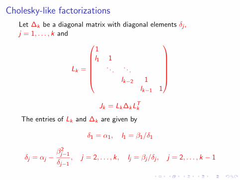
Let ∆k be a diagonal matrix with diagonal elements δj ,j = 1, . . . , k and
Lk =
1l1 1
. . .. . .
lk−2 1lk−1 1
Jk = Lk∆kLT
k
The entries of Lk and ∆k are given by
δ1 = α1, l1 = β1/δ1
δj = αj −β2
j−1
δj−1, j = 2, . . . , k, lj = βj/δj , j = 2, . . . , k − 1

The factorization can be completed if no δj is zero forj = 1, . . . , k − 1
This does not happen if Jk is positive definite, all the elements δj
are positive and the genuine Cholesky factorization can beobtained from ∆k
Jk = LCk (LC
k )T
with LCk = Lk∆
1/2k which is
LCk =
√δ1
β1√δ1
√δ2
. . .. . .
βk−2√δk−2
√δk−1
βk−1√δk−1
√δk

The factorization can also be written as
Jk = LDk ∆−1
k (LDk )T
with
LDk =
δ1
β1 δ2
. . .. . .
βk−2 δk−1
βk−1 δk
Clearly, the only elements we have to compute and store are the
diagonal elements δj , j = 1, . . . , k
To solve a linear system Jkx = c , we successively solve
LDk y = c , (LD
k )T x = ∆ky

The previous factorizations proceed from top to bottom (LU)We can also proceed from bottom to top (UL)
Jk = LTk D−1
k Lk
with
Lk =
d
(k)1
β1 d(k)2. . .
. . .
βk−2 d(k)k−1
βk−1 d(k)k
and Dk a diagonal matrix with elements d
(k)j
d(k)k = αk , d
(k)j = αj −
β2j
d(k)j+1
, j = k − 1, . . . , 1

From LU and UL factorizations we can obtain all the so-called“twisted” factorizations of Jk
Jk = MkΩkMTk
Mk is lower bidiagonal at the top for rows with index smaller thanl and upper bidiagonal at the bottom for rows with index largerthan l
ω1 = α1, ωj = αj −β2
j−1
ωj−1, j = 2, . . . , l − 1
ωk = αk , ωj = αj −β2
j
ωj+1, j = k − 1, . . . , l + 1
ωl = αl −β2
l−1
ωl−1−
β2l
ωl+1
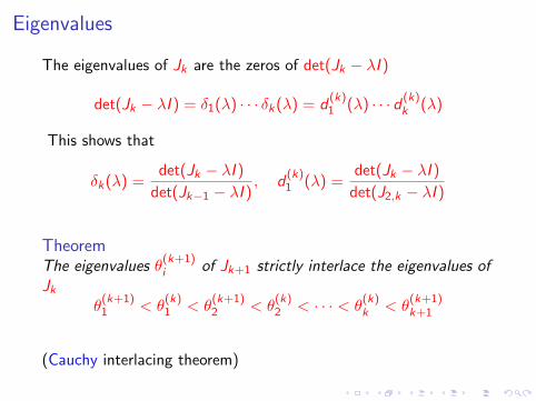
Eigenvalues
The eigenvalues of Jk are the zeros of det(Jk − λI )
det(Jk − λI ) = δ1(λ) · · · δk(λ) = d(k)1 (λ) · · · d (k)
k (λ)
This shows that
δk(λ) =det(Jk − λI )
det(Jk−1 − λI ), d
(k)1 (λ) =
det(Jk − λI )
det(J2,k − λI )
TheoremThe eigenvalues θ
(k+1)i of Jk+1 strictly interlace the eigenvalues of
Jk
θ(k+1)1 < θ
(k)1 < θ
(k+1)2 < θ
(k)2 < · · · < θ
(k)k < θ
(k+1)k+1
(Cauchy interlacing theorem)
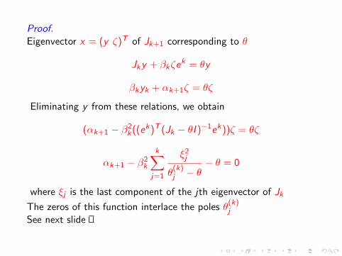
Proof.Eigenvector x = (y ζ)T of Jk+1 corresponding to θ
Jky + βkζek = θy
βkyk + αk+1ζ = θζ
Eliminating y from these relations, we obtain
(αk+1 − β2k((ek)T (Jk − θI )−1ek))ζ = θζ
αk+1 − β2k
k∑j=1
ξ2j
θ(k)j − θ
− θ = 0
where ξj is the last component of the jth eigenvector of Jk
The zeros of this function interlace the poles θ(k)j
See next slide
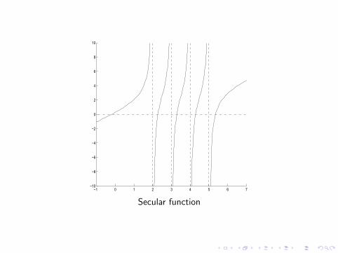
−1 0 1 2 3 4 5 6 7−10
−8
−6
−4
−2
0
2
4
6
8
10
Secular function

Results on eigenvector components
Let χj ,k(λ) be the determinant of Jj ,k − λI
The first components of the eigenvectors z i of Jk are
(z i1)
2 =
∣∣∣∣∣∣χ2,k(θ(k)i )
χ′1,k(θ(k)i )
∣∣∣∣∣∣ ,that is,
(z i1)
2 =θ(k)i − θ
(2,k)1
θ(k)i − θ
(k)1
· · ·θ(k)i − θ
(2,k)i−1
θ(k)i − θ
(k)i−1
θ(2,k)i − θ
(k)i
θ(k)i+1 − θ
(k)i
· · ·θ(2,k)k−1 − θ
(k)i
θ(k)k − θ
(k)i
.
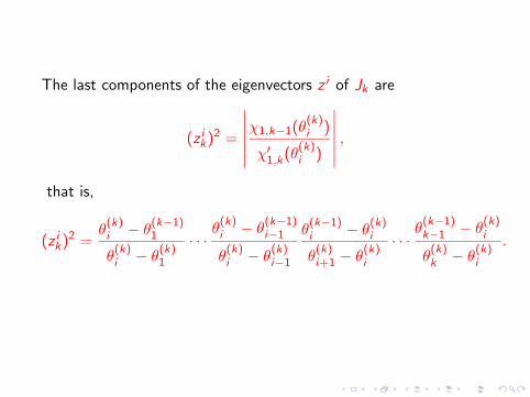
The last components of the eigenvectors z i of Jk are
(z ik)2 =
∣∣∣∣∣∣χ1,k−1(θ(k)i )
χ′1,k(θ(k)i )
∣∣∣∣∣∣ ,that is,
(z ik)2 =
θ(k)i − θ
(k−1)1
θ(k)i − θ
(k)1
· · ·θ(k)i − θ
(k−1)i−1
θ(k)i − θ
(k)i−1
θ(k−1)i − θ
(k)i
θ(k)i+1 − θ
(k)i
· · ·θ(k−1)k−1 − θ
(k)i
θ(k)k − θ
(k)i
.
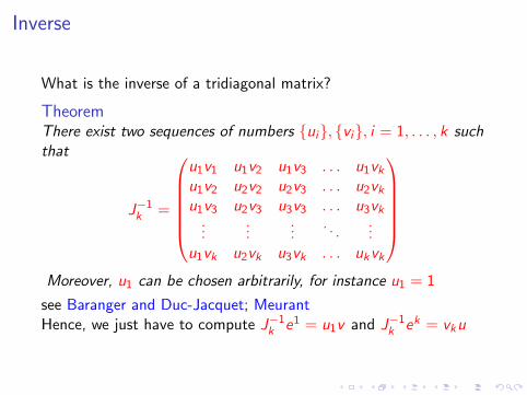
Inverse
What is the inverse of a tridiagonal matrix?
TheoremThere exist two sequences of numbers ui, vi, i = 1, . . . , k suchthat
J−1k =
u1v1 u1v2 u1v3 . . . u1vk
u1v2 u2v2 u2v3 . . . u2vk
u1v3 u2v3 u3v3 . . . u3vk...
......
. . ....
u1vk u2vk u3vk . . . ukvk
Moreover, u1 can be chosen arbitrarily, for instance u1 = 1
see Baranger and Duc-Jacquet; MeurantHence, we just have to compute J−1
k e1 = u1v and J−1k ek = vku
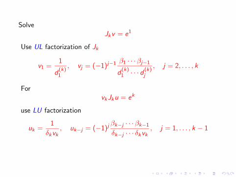
SolveJkv = e1
Use UL factorization of Jk
v1 =1
d(k)1
, vj = (−1)j−1 β1 · · ·βj−1
d(k)1 · · · d (k)
j
, j = 2, . . . , k
ForvkJku = ek
use LU factorization
uk =1
δkvk, uk−j = (−1)j
βk−j · · ·βk−1
δk−j · · · δkvk, j = 1, . . . , k − 1

TheoremThe inverse of the symmetric tridiagonal matrix Jk is characterizedas
(J−1k )i ,j = (−1)j−iβi · · ·βj−1
d(k)j+1 · · · d
(k)k
δi · · · δk, ∀i , ∀j > i
(J−1k )i ,i =
d(k)i+1 · · · d
(k)k
δi · · · δk, ∀i
Proof.
ui = (−1)−(i+1) 1
β1 · · ·βi−1
d(k)1 · · · d (k)
k
δi · · · δk
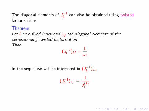
The diagonal elements of J−1k can also be obtained using twisted
factorizations
TheoremLet l be a fixed index and ωj the diagonal elements of thecorresponding twisted factorizationThen
(J−1k )l ,l =
1
ωl
In the sequel we will be interested in (J−1k )1,1
(J−1k )1,1 =
1
d(k)1

The (1,1) entry of the inverse
Can we compute (J−1k )1,1 incrementally?
Theorem
(J−1k+1)1,1 = (J−1
k )1,1 +(β1 · · ·βk)2
(δ1 · · · δk)2δk+1
Proof.
Jk+1 =
(Jk βkek
βk(ek)T αk+1
)The upper left block of J−1
k+1 is the inverse of the Schurcomplement (
Jk −β2
k
αk+1ek(ek)T
)−1
Inverse of a rank-1 modification of Jk
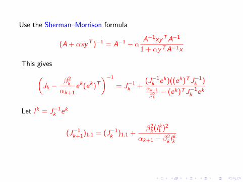
Use the Sherman–Morrison formula
(A + αxyT )−1 = A−1 − αA−1xyTA−1
1 + αyTA−1x
This gives(Jk −
β2k
αk+1ek(ek)T
)−1
= J−1k +
(J−1k ek)((ek)T J−1
k )αk+1
β2k− (ek)T J−1
k ek
Let lk = J−1k ek
(J−1k+1)1,1 = (J−1
k )1,1 +β2
k(lk1 )2
αk+1 − β2k lkk
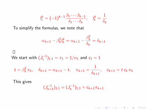
lk1 = (−1)k−1 β1 · · ·βk−1
δ1 · · · δk, lkk =
1
δk
To simplify the formulas, we note that
αk+1 − β2k lkk = αk+1 −
β2k
δk= δk+1
We start with (J−11 )1,1 = π1 = 1/α1 and c1 = 1
t = β2k πk , δk+1 = αk+1 − t, πk+1 =
1
δk+1, ck+1 = t ck πk
This gives(J−1
k+1)1,1 = (J−1k )1,1 + ck+1πk+1
The QD algorithm
The QD algorithm is a method introduced by Heinz Rutishauser tocompute the eigenvalues of a tridiagonal matrix
See also Stiefel, Henrici, Fernando and Parlett, Parlett and Laurie
Let us start with the LR algorithm
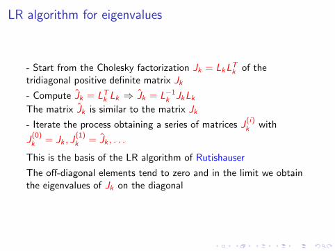
LR algorithm for eigenvalues
- Start from the Cholesky factorization Jk = LkLTk of the
tridiagonal positive definite matrix Jk
- Compute Jk = LTk Lk ⇒ Jk = L−1
k JkLk
The matrix Jk is similar to the matrix Jk
- Iterate the process obtaining a series of matrices J(i)k with
J(0)k = Jk , J
(1)k = Jk , . . .
This is the basis of the LR algorithm of Rutishauser
The off-diagonal elements tend to zero and in the limit we obtainthe eigenvalues of Jk on the diagonal

Can we compute Lk , the Cholesky factor of Jk = LTk Lk without
explicitly computing Jk?
We have
Jk =
δ1 +β2
1δ1
β1
√δ2δ1
β1
√δ2δ1
δ2 +β2
2δ2
β2
√δ3δ2
. . .. . .
. . .
βk−2
√δk−1
δk−2δk−1 +
β2k−1
δk−1βk−1
√δk
δk−1
βk−1
√δk
δk−1δk
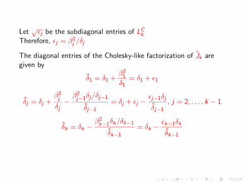
Let√
εj be the subdiagonal entries of LCk
Therefore, εj = β2j /δj
The diagonal entries of the Cholesky-like factorization of Jk aregiven by
δ1 = δ1 +β2
1
δ1= δ1 + ε1
δj = δj +β2
j
δj−
β2j−1δj/δj−1
δj−1
= δj + εj −εj−1δj
δj−1
, j = 2, . . . , k − 1
δk = δk −β2
k−1δk/δk−1
δk−1
= δk −εk−1δk
δk−1

Let εj = β2j δj+1/(δj δj)
The diagonal entries of Lk are√
δj , the subdiagonal entries are√εj and
εj = εjδj+1
δj
The expression for δj can be written as
δj = δj + εj − εj−1
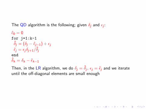
The QD algorithm is the following; given δj and εj :
ε0 = 0for j=1:k-1δj = (δj − εj−1) + εjεj = εjδj+1/δj
endδk = δk − εk−1
Then, in the LR algorithm, we do δj = δj , εj = εj and we iterateuntil the off-diagonal elements are small enough
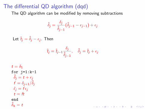
The differential QD algorithm (dqd)The QD algorithm can be modified by removing subtractions
δj =δj
δj−1
(δj−1 − εj−1) + εj
Let tj = δj − εj . Then
tj = tj−1δj
δj−1
, δj = tj + εj
t = δ1
for j=1:k-1δj = t + εjf = δj+1/δj
εj = f εjt = ft
endδk = t

The differential QD algorithm with shift
The algorithm with shift dqds(µ) is:
t = δ1 − µfor j=1:k-1δj = t + εjf = δj+1/δj
εj = f εjt = ft − µ
endδk = t
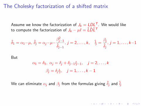
The Cholesky factorization of a shifted matrix
Assume we know the factorization of Jk = LDLT . We would liketo compute the factorization of Jk − µI = LDLT
δ1 = α1−µ, δj = αj−µ−β2
j−1
δj−1
, j = 2, . . . , k, lj =βj
δj
, j = 1, . . . , k−1
Butα1 = δ1, αj = δj + δj−1lj−1, j = 2, . . . , k
βj = δj lj , j = 1, . . . , k − 1
We can eliminate αj and βj from the formulas giving δj and lj
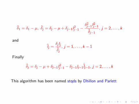
δ1 = δ1 − µ, δj = δj − µ + δj−1l2j−1 −
δ2j−1l
2j−1
δj−1
, j = 2, . . . , k
and
lj =δj lj
δj
, j = 1, . . . , k − 1
Finally
δj = δj − µ + δj−1l2j−1 − δj−1lj−1 lj−1, j = 2, . . . , k
This algorithm has been named stqds by Dhillon and Parlett
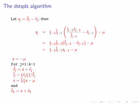
The dstqds algorithm
Let sj = δj − δj ; then
sj = lj−1 lj−1
(lj−1δj−1
lj−1
− δj−1
)− µ
= lj−1 lj−1(δj−1 − δj−1)− µ
= lj−1 lj−1sj−1 − µ
s = −µfor j=1:k-1δj = s + δj
lj = (δj lj)/δj
s = lj ljs − µendδk = s + δk

Historical note
I Augustin Louis Cauchy, (1789 Paris, France-1857 Sceaux,France), French mathematician
I Issai Schur, (1875 Mogilev, Russia-1941 Tel Aviv, Israel),German mathematician
I Andre-Louis Cholesky, (1875 Montguyon, France-1918Bagneux (Soissons), France), French geodesist
I Eduard Ludwig Stiefel, (1909-1978 Zurich, Switzerland),Swiss mathematician
I Heinz Rutishauser, (1918 Weinfelden, Switzerland-1970Zurich, Swtizerland), Swiss mathematician
I Peter Henrici, (1923 Basel, Switzerland-1987 Zurich,Switzerland), Swiss mathematician
I Jack Sherman, (?), American statistician
I Winifred J. Morrison, (?), American statistician
I Beresford Neill Parlett, (? ?-), American mathematician
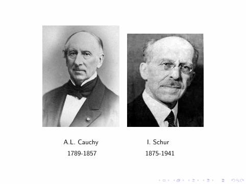
A.L. Cauchy I. Schur
1789-1857 1875-1941

A-L. Cholesky
1875-1918

H. Rutishauser E. Stiefel
1918-1970 1909-1978
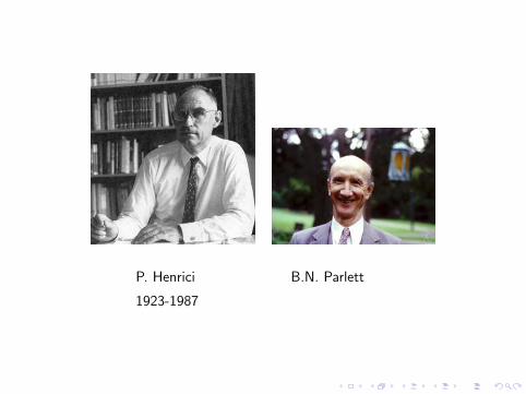
P. Henrici B.N. Parlett
1923-1987

J. Baranger and M. Duc-Jacquet, Matricestridiagonales symetriques et matrices factorisables, RIRO, v 3(1971), pp. 61–66
I.S. Dhillon and B.N. Parlett, Relatively robustrepresentations of symmetric tridiagonals, Linear Alg. Appl.,v 309 (2000), pp. 121–151
K.V. Fernando and B.N. Parlett, Accurate singularvalues and differential qd algorithms, Numer. Math., v 67(1994), pp. 191–229
G.H. Golub and C. Van Loan, Matrix Computations,Third Edition, Johns Hopkins University Press, (1996)
P. Henrici, The quotient-difference algorithm, NBSAppl. Math. Series, v 49 (1958), pp. 23–46
G. Meurant, A review of the inverse of tridiagonal andblock tridiagonal matrices, SIAM J. Matrix Anal. Appl., v 13n 3 (1992), pp. 707–728

B.N. Parlett, The new qd algorithms, Acta Numerica, v 15(1995), pp. 459-491
H. Rutishauser, Der Quotienten-Differenzen-Algorithmus,Zeitschrift fur Angewandte Mathematik und Physik (ZAMP),v 5 n 3 (1954), pp. 233-251
H. Rutishauser, Solution of eigenvalue problems with theLR-transformation , Nat. Bur. Standards Appl. Math. Ser.,v 49 (1958), pp. 47–81