chapter 24: strategic energy management (sem) evaluation ... · 7.2.1 pre-post method 45¶ ......

NREL is a national laboratory of the U.S. Department of Energy Office of Energy Efficiency & Renewable Energy Operated by the Alliance for Sustainable Energy, LLC This report is available at no cost from the National Renewable Energy Laboratory (NREL) at www.nrel.gov/publications.

Chapter XX: Strategic Energy Management (SEM) Evaluation Protocol [DRAFT v6] The Uniform Methods Project: Methods for Determining Energy Efficiency Savings for Specific Measures Created as part of subcontract with period of performance September 2011 – July 2016 James Stewart, Ph.D. The Cadmus Group Portland, Oregon

NREL Technical Monitor: Charles Kurnik

Subcontract Report NREL/XX-XXXX-XXXXX July 2016

Deleted: – Steering Committee review

NREL is a national laboratory of the U.S. Department of Energy Office of Energy Efficiency & Renewable Energy Operated by the Alliance for Sustainable Energy, LLC Thi t i il bl t t f th N ti l R bl E

Contract No. DE-AC36-08GO28308

National Renewable Energy Laboratory 15013 Denver West Parkway Golden, CO 80401 303-275-3000 • www.nrel.gov

Chapter XX: Strategic Energy Management (SEM) Evaluation Protocol [DRAFT v6] The Uniform Methods Project: Methods for Determining Energy Efficiency Savings for Specific Measures Created as part of subcontract with period of performance September 2011 – July 2016 James Stewart, Ph.D. The Cadmus Group Portland, Oregon

NREL Technical Monitor: Charles Kurnik Prepared under Subcontract No. LGJ-1-11965-01

Subcontract Report NREL/XX-XXXX-XXXXX July 2016

Deleted: 4 – Steering Committee review

NOTICE

This report was prepared as an account of work sponsored by an agency of the United States government. Neither the United States government nor any agency thereof, nor any of their employees, makes any warranty, express or implied, or assumes any legal liability or responsibility for the accuracy, completeness, or usefulness of any information, apparatus, product, or process disclosed, or represents that its use would not infringe privately owned rights. Reference herein to any specific commercial product, process, or service by trade name, trademark, manufacturer, or otherwise does not necessarily constitute or imply its endorsement, recommendation, or favoring by the United States government or any agency thereof. The views and opinions of authors expressed herein do not necessarily state or reflect those of the United States government or any agency thereof.

This report is available at no cost from the National Renewable Energy Laboratory (NREL) at http://www.nrel.gov/research/publications.html.

Available electronically at http://www.osti.gov/scitech

Available for a processing fee to U.S. Department of Energy and its contractors, in paper, from:

U.S. Department of Energy Office of Scientific and Technical Information P.O. Box 62 Oak Ridge, TN 37831-0062 phone: 865.576.8401 fax: 865.576.5728 email: mailto:[email protected]

Available for sale to the public, in paper, from:

U.S. Department of Commerce National Technical Information Service 5285 Port Royal Road Springfield, VA 22161 phone: 800.553.6847 fax: 703.605.6900 email: [email protected] online ordering: http://www.ntis.gov/help/ordermethods.aspx

Cover Photos: (left to right) photo by Pat Corkery, NREL 16416, photo from SunEdison, NREL 17423, photo by Pat Corkery, NREL 16560, photo by Dennis Schroeder, NREL 17613, photo by Dean Armstrong, NREL 17436, photo by Pat Corkery, NREL 17721.

NREL prints on paper that contains recycled content.

http://www.nrel.gov/research/publications.html

http://www.osti.gov/scitech

mailto:[email protected]

mailto:[email protected]

http://www.ntis.gov/help/ordermethods.aspx

i

Acknowledgments The chapter author wishes to thank and acknowledge the following individuals for their thoughtful comments and suggestions on drafts of this protocol: Marc Collins of Itron; Miriam Goldberg, Andrew Styker, and Julia Vetromile of DNV-GL; Kim Crossman, Erika Kociolek, and Phil Degens of Energy Trust of Oregon; Deborah Swarts of Navigant; Bill Miller, Aimee McKane, Darren Sholes, Peter Therkelsen, and Shankar Earni of LBNL; Paul Scheihing and Jay Wrobel, of the U.S. Department of Energy; Jim Volkman of Strategic Energy Group; Todd Amundson, Lauren Gage, Steve Brooks, and Jennifer Eskil of the Bonneville Power Administration; Steve Martin of Cascade Energy Engineering; Bill Koran of SBW Consulting; and Hossein Haeri, M. Sami Khawaja, Jeff Cropp, Jennifer Huckett, Heidi Javanbakht, and Andrew Bernath of Cadmus.

In addition, the chapter author wishes to acknowledge helpful comments submitted through the public comment process from Bill Harris of Snohomish Public Utility District, Jess Burgess of the Consortium for Energy Efficiency, and the American Water Works Association.

Deleted: for their thoughtful comments and suggestions on drafts of this protocol

Formatted: Not Highlight

Formatted: Not HighlightDeleted:

ii

Acronyms BPA Bonneville Power Administration

Btu British thermal unit

CDD Cooling degree day

DOE Department of Energy

EM&V Evaluation, Measurement and Verification

EUI Energy use intensity

HDD Heating degree day

HVAC Heating, ventilation, and air conditioning

IPMVP International Performance Measurement and Verification Protocol

ISO 50001 International Organization for Standardization (ISO) for an Energy Management System

M&V Measurement and Verification

OLS Ordinary least squares

OM&B Operation, maintenance, and behavior

PE Program Evaluation

SEM Strategic Energy Management

SEP Superior Energy Performance

UMP Uniform Methods Project

iii

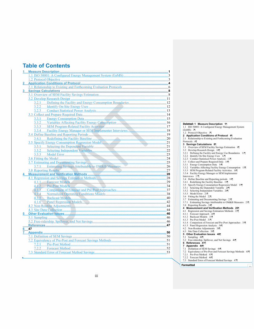
Table of Contents 1 Measure Description ............................................................................................................................ 1

1.1 ISO 50001: A Configured Energy Management System (EnMS) ................................................. 3 1.2 Protocol Objective ...................................................................................................................... 3

2 Application Conditions of Protocol .................................................................................................... 4 2.1 Relationship to Existing and Forthcoming Evaluation Protocols .................................................. 6

3 Savings Calculations ........................................................................................................................... 8 3.1 Overview of SEM Facility Savings Estimation ............................................................................ 8 3.2 Develop Research Design ......................................................................................................... 11

3.2.1 Defining the Facility and Energy Consumption Boundaries ......................................... 12 3.2.2 Identify On-Site Energy Uses ..................................................................................... 12 3.2.3 Conduct Statistical Power Analysis ............................................................................. 13

3.3 Collect and Prepare Required Data ............................................................................................ 14 3.3.1 Energy Consumption Data .......................................................................................... 15 3.3.2 Variables Affecting Facility Energy Consumption ...................................................... 16 3.3.3 SEM Program-Related Facility Activities ................................................................... 17 3.3.4 Facility Energy Manager or SEM Implementer Interviews .......................................... 18

3.4 Define Baseline and Reporting Periods ..................................................................................... 19 3.4.1 Redefining the Facility Baseline ................................................................................. 20

3.5 Specify Energy Consumption Regression Model ....................................................................... 21 3.5.1 Selecting the Dependent Variable ............................................................................... 21 3.5.2 Selecting Independent Variables ................................................................................. 22 3.5.3 Model Error ................................................................................................................ 23

3.6 Fitting the Model ...................................................................................................................... 24 3.7 Estimating and Documenting Savings ....................................................................................... 25

3.7.1 Estimating Savings Attributable to OM&B Measures .................................................. 26 3.8 Reporting Results...................................................................................................................... 27

4 Measurement and Verification Methods .......................................................................................... 28 4.1 Regression and Savings Estimation Methods ............................................................................. 28

4.1.1 Forecast Models ......................................................................................................... 29 4.1.2 Pre-Post Models ......................................................................................................... 34 4.1.3 Comparison of Forecast and Pre-Post Approaches....................................................... 37 4.1.4 Normalized Operating Conditions Models .................................................................. 38 4.1.5 Backcast Models ......................................................................................................... 40 4.1.6 Panel Regression Models ............................................................................................ 42

4.2 Non-Routine Adjustments ......................................................................................................... 44 4.3 Site Data Collection .................................................................................................................. 44

5 Other Evaluation Issues ..................................................................................................................... 46 5.1 Sampling .................................................................................................................................. 46 5.2 Free-ridership, Spillover, and Net Savings................................................................................. 46

References .......................................................................................................................................... 47 6 47 7 Appendix ............................................................................................................................................. 50

7.1 Definition of SEM Savings ....................................................................................................... 50 7.2 Equivalency of Pre-Post and Forecast Savings Methods ............................................................ 51

7.2.1 Pre-Post Method ......................................................................................................... 51 7.2.2 Forecast Method ......................................................................................................... 52

7.3 Standard Error of Forecast Method Savings............................................................................... 53

Deleted: 1 Measure Description 1¶1.1 ISO 50001: A Configured Energy Management System (EnMS) 3¶1.2 Protocol Objective 3¶2 Application Conditions of Protocol 4¶2.1 Relationship to Existing and Forthcoming Evaluation Protocols 6¶3 Savings Calculations 8¶3.1 Overview of SEM Facility Savings Estimation 8¶3.2 Develop Research Design 10¶3.2.1 Defining the Facility and Energy Use Boundaries 11¶3.2.2 Identify On-Site Energy Uses 12¶3.2.3 Conduct Statistical Power Analysis 13¶3.3 Collect and Prepare Required Data 14¶3.3.1 Energy Consumption Data 14¶3.3.2 Variables Affecting Facility Energy Consumption 15¶3.3.3 SEM Program-Related Facility Activities 16¶3.3.4 Facility Energy Manager or SEM Implementer Interviews 17¶3.4 Define Baseline and Reporting periods 18¶3.4.1 Redefining the Facility Baseline 19¶3.5 Specify Energy Consumption Regression Model 19¶3.5.1 Selecting the Dependent Variable 20¶3.5.2 Selecting Independent Variables 20¶3.5.3 Model Error 21¶3.6 Fitting the Model 22¶3.7 Estimating and Documenting Savings 23¶3.7.1 Estimating Savings Attributable to OM&B Measures 23¶3.8 Reporting Results 24¶4 Measurement and Verification Methods 25¶4.1 Regression and Savings Estimation Methods 25¶4.1.1 Forecast Approach 26¶4.1.2 Backcast Models 31¶4.1.3 Pre-Post Model 31¶4.1.4 Comparison of Forecast and Pre-Post Approaches 35¶4.1.5 Panel Regression Analysis 36¶4.2 Non-Routine Adjustments 38¶4.3 Site Data Collection 38¶5 Other Evaluation Issues 40¶5.1 Sampling 40¶5.2 Free-ridership, Spillover, and Net Savings 40¶6 References 41¶7 Appendix 44¶7.1 Definition of SEM Savings 44¶7.2 Equivalency of Pre-Post and Forecast Savings Methods 45¶7.2.1 Pre-Post Method 45¶7.2.2 Forecast Method 46¶7.3 Standard Error of Forecast Method Savings 47¶

Formatted ...

iv

List of Figures Figure 1. Estimation of SEM Energy Savings .......................................................................................... 9 Figure 2. Plot of SEM Facility Electricity Consumption and Output vs. Time .................................... 32

List of Tables Table 1. Example Industrial Facility Energy Consumption and Output Data ..................................... 31 Table 2. Estimates of Facility Forecast Regression Model ................................................................... 33 Table 3. Estimates of Facility Adjusted Baseline Energy Consumption and Savings ...................... 33 Table 4. Pre-Post Regression Model Estimates ..................................................................................... 36 Table 5. Reporting Period Regression Model Estimates ...................................................................... 40 Table 6. Normalized Operating Conditions Savings Estimate ............................................................. 40 Table 7. Backcast Model Savings Estimates ......................................................................................... 41

Deleted: Figure 1. Estimation of SEM Energy Savings 7¶Figure 2. Plot of SEM Facility Electricity Use and Output vs. Time 25¶

Formatted: Default Paragraph Font, Font: (Default) +Body(Times New Roman), 11 pt, Not Bold, Font color: Text 1,Check spelling and grammar


Deleted: Table 1. Example Industrial Facility Energy Use and Output Data 25¶Table 2. Estimates of Facility Forecast Regression Model 26¶Table 3. Estimates of Monthly Facility Adjusted Baseline Energy Use and Savings 27¶Table 4. Pre-Post Facility Energy Use Regression Model Estimates 30¶





1

1 Measure Description Strategic Energy Management (SEM) focuses on achieving energy-efficiency improvements through systematic and planned changes in facility operations, maintenance, and behaviors (OM&B) and capital equipment upgrades in large energy-using facilities, including industrial buildings, commercial buildings, and multi-facility organizations such as campuses or communities. Facilities can institute a spectrum of SEM actions, ranging from a simple process for regularly identifying energy-savings actions, to establishing a formal, third-party recognized or certified SEM framework for continuous improvement of energy performance. In general, SEM programs that would be considered part of a utility program will contain a set of energy-reducing goals, principles, and practices emphasizing continuous improvements in energy performance or savings through energy management and an energy management system (EnMS). An EnMS as defined by ISO 50001, is a formalized process for an organization to establish a policy, objectives, and targets for energy performance improvement and to implement and to assess energy performance improvement actions taken to meet those objectives and targets. An organization uses this framework to incorporate energy use and consumption into its management processes.

To provide some guidance to utilities in consideration of SEM programs, the Consortium for Energy Efficiency (CEE) has established a working definition for SEM as follows:

“Strategic Energy Management can be defined as taking a holistic approach to managing energy use in order to continuously improve energy performance, by achieving persistent energy and cost savings over the long term. It focuses on business practice change from senior management to the shop floor staff, affecting organizational culture to reduce energy waste and improve energy intensity. SEM emphasizes equipping and enabling plant management and staff to impact energy consumption through behavioral and operational change. While SEM does not emphasize a technical or project centric approach, SEM principles and objectives may support capital project implementation.” (CEE 2014a)

The CEE developed a set of three SEM Minimum Elements–customer commitment, planning and implementation, and a measurement and reporting system–supported by thirteen specific components of industrial SEM (“CEE SEM minimum elements”) and specific responsibilities for senior managers and the energy management team, though not every SEM industrial program incorporates all of these components:

Senior management:

1. Sets and communicates long-range energy performance goals. 2. Ensures that SEM initiatives are sufficiently resourced and a responsible individual or

team designated. Designated energy manager or management team:

Deleted: simply

Deleted:

Deleted: program

Deleted: , to making large scale capital

Deleted: improvements

Deleted: in energy using infrastructure

Deleted:

Deleted: identify and plan for

Deleted: s

Deleted: over a longer time horizon

Deleted: It

Deleted: a system of management practices

Deleted: use

Deleted: the organization’s

Deleted: list of 13 elements

Deleted: programs

Deleted: ,

Deleted: though not every SEM industrial program incorporates each of these

2

3. Assesses current energy management practices using a performance scorecard or facilitated energy management assessment.

4. Develops a map of energy use, consumption and cost, including all significant end use systems and relevant variables of energy consumption.

5. Establishes clear, measurable metrics and goals for energy performance improvement. 6. Registers or records actions to be undertaken to achieve the energy performance goals. 7. Develops and implements a plan to engage employees in energy performance

improvement 8. Implements planned actions. 9. Periodically reassesses outcomes related to energy performance. 10. Regularly collects performance data to improve understanding of energy use and

consumption. 11. Collects and stores performance data related to energy performance improvement metrics

and goals, making it available over time. 12. Analyzes energy use and consumption data, determining relevant variables affecting use

compared to a baseline.

13. Reports regularly to senior management and others on results of energy performance improvement actions.

While CEE developed this list for industrial facilities, the SEM minimum elements also apply to management of energy use in commercial and institutional buildings, multi-facility organizations, and campus settings. Currently, many utilities and program administrators offer ratepayer-funded SEM programs that enroll a range of industrial, commercial and institutional customers (CEE 2016).1 These utility administered programs each provide a distinct program design for qualifying participants, which contain some of the CEE elements. Most programs provide participating facilities or organizations with training about energy management practices and EnMS, technical support for implementation, and financial incentives for achieving energy savings, with the objective of integrating SEM into facility or building operations. Many utility SEM programs expect to save 5% or more of annual facility energy consumption by helping participants to implement these SEM elements (CEE 2014). To acquire savings, utility SEM programs support participants’ capability for continuously improving energy performance through adoption of SEM practices.2

1 CEE (2016) identifies 25 member utilities or program administrators in the United States and Canada that fund industrial SEM programs. 2 SEM Program Case Studies Report (CEE 2015).

Formatted: Numbered + Level: 1 + Numbering Style: 1, 2,3, … + Start at: 1 + Alignment: Left + Aligned at: 0.25" +Tab after: 0.5" + Indent at: 0.5"

Deleted: ¶

Deleted: with minor modification

Deleted: large

Deleted: or

Deleted: 2014b

Deleted: participation of

Deleted: customers

Deleted: to

Deleted: implement SEM activities

Deleted: A smaller, and expanding, number of programs include most of the CEE elements or focus on the establishment of the EnMS to improve customer engagement or achieve greater energy savings over time.

Formatted: Space After: 10 ptDeleted: use

Deleted: ing

Deleted: with the intention that on-going energy management would become a fixed practice at the participating sites

Formatted: Font: 11 pt

Formatted: Font: 11 ptDeleted: 2014b

Deleted: lists

Deleted: 11

Deleted:



3

1.1 ISO 50001: A Configured Energy Management System (EnMS) SEM programs fall on a continuum, from those meeting the minimum elements noted above to those that also meet or exceed the requirements of the ISO 50001 Energy Management System standard. ISO 50001 is an international standard with a defined ‘plan-do-check-act' EnMS that sets forth a series of organizational practices to effectively manage energy and continually improve energy performance. ISO 50001 also includes methods for calculating period-over-period changes in energy performance and requires documented evidence of energy performance improvement. Since ISO 50001 is user-administered, organizations seeking ISO 50001 certification are subject to a certification audit conducted by a qualified audit team from a nationally accredited certification body.3

An application of an ISO 50001-conformant EnMS is the U.S. Department of Energy’s (DOE) Superior Energy Performance (SEP). SEP builds upon the ISO 50001 by applying the Superior Energy Performance Measurement and Verification Protocol (DOE 2016c) across all energy types to meet specific targets over defined periods of time for measurement and verification of energy performance improvement. In addition, the U.S. Department of Energy’s (DOE) has developed the 50001 Ready program, which follows the Qualified Energy Savings (QES) Protocol (DOE, 2017a) and will provide DOE (and/or partner) recognition for self-declared conformance to ISO 50001. The 50001 Ready program will provide energy and carbon emissions savings calculation and is designed to partner with utilities and other organizations, including state and local governments or multi-facility organizations to support their ‘enterprise’ of facilities or their supply chain.

1.2 Protocol Objective This protocol’s objective is to help program evaluators and administrators accurately assess the gross energy savings of utility SEM programs. This protocol focuses on best practices for estimating energy savings for individual large commercial or industrial facilities, although the protocol also describes methods for conducting analysis to estimate the average savings per facility for a group of facilities.4

As utility SEM programs are a relatively new offering, evaluators are still developing best practices for evaluation. This protocol describes current thinking about best practices, but it is expected that this protocol will require updating as evaluation approaches improve and consensus builds around the best approaches.

3 ANSI-ASQ National Accreditation Board (ANAB). More complete information on ISO 50001 can be found at http://www.energy.gov/eere/amo/iso-50001-frequently-asked-questions 4 Estimation of average savings for groups of facilities, or “panels” is presented in section 4. For estimation of energy savings from small commercial buildings, see NREL (Agnew 2013).





Deleted: energy performance improvement

Deleted: panel

Deleted: current

Formatted: NREL_Body_Text, Space After: 0 pt, Linespacing: singleDeleted: ¶





4

2 Application Conditions of Protocol For the purpose of providing guidance about evaluating SEM programs, this protocol differentiates between three categories of SEM programs. The first category includes those that satisfy some or all of the CEE definition of SEM. The second category includes those that require all of the CEE elements and promote the establishment of an ISO 50001-conformant EnMS. The third category includes those programs that further promote certification to SEP.

This UMP protocol provides guidance for evaluating the savings impacts of SEM programs administered by utilities or other energy efficiency organizations. This protocol applies to all utility SEM programs whether or not they satisfy all of the CEE minimum elements. For utility or energy efficiency organization programs designed to conform with ISO 50001, this Protocol incorporates by reference and directs evaluators to use US DOE’s Qualified Energy Savings (QES) Protocol (DOE 2017a). For utility or energy efficiency organization programs designed to conform to SEP, this Protocol incorporates by reference and directs evaluators to use the Superior Energy Performance Measurement and Verification Protocol (DOE 2016c).

For utility SEM programs that satisfy some or all of the CEE SEM elements, this protocol recommends statistical analysis of metered facility energy consumption for estimating energy savings. A facility is the analysis unit of SEM program impact evaluations and the area over which energy use and consumption will be measured and analyzed. A facility may comprise a single building with a single meter or multiple buildings at the same site with multiple energy use meters.5 The reporting period is when energy savings from SEM activity will be estimated. The baseline period is when energy consumption measurements are taken to establish a baseline for the facility’s energy consumption.

Evaluators should apply this protocol when all of the following conditions are satisfied:

• Estimating changes in a facility’s energy consumption6 (savings) or energy consumption intensity (energy consumption per unit of production output or unit of floor area) from SEM activities is the evaluation objective. Estimation of peak demand savings is not covered. While many SEM programs deliver peak demand savings, estimating these

5 This definition of a facility will apply to most participants in utility SEM programs; however, some participants such as water utilities and waste water treatment facilities have complex distribution and pumping systems that do not have simple boundaries. Many opportunities for reducing energy consumption through SEM may exist in their distribution networks. The definition of facility is not intended to preclude the participation of water utilities in utility SEM programs or opportunities for them to save energy through distribution system efficiency improvements. 6 Depending on the SEM program and evaluation objectives, a facility’s energy use may include consumption of a single fuel or multiple fuels. Evaluation of savings for multiple fuels is discussed in Section 4.

Formatted: Font: Italic

Deleted: with some additional requirements described in Section 3…

Deleted: 2016




5

savings requires different data and analysis methods from those presented in this protocol.7

• Facility-level data on energy consumption, production output,8 and weather9 for industrial facilities or on energy consumption, weather, floor area, and occupancy or utilization for large commercial buildings are available for the baseline and reporting periods. Analysis of facility energy consumption, as opposed to analysis of end-use consumption, is recommended for several reasons. First, SEM often affects multiple energy end uses; so only by analyzing whole-facility energy consumption data can evaluators be sure to measure all SEM savings. Second, even if all affected energy end uses could be identified, individual metering may be prohibitively costly. Third, there may be interactive effects between SEM activities that are not recognized or difficult to measure. Again, facility energy consumption will capture all of the interactive effects. In addition to facility energy consumption, data on the principal drivers of facility energy consumption, such as output and weather, must also be available for the baseline and SEM reporting periods to perform the savings analysis.

• Evaluators have sufficient understanding of energy consumption at the facility to construct a valid facility energy consumption model. Evaluators must also understand the relationships between facility energy consumption and the principal drivers of energy consumption to develop valid energy consumption models. Incomplete understanding increases the risk of incorrectly specifying the baseline regression model. Often, information about facility energy consumption and SEM program activities can be obtained through SEM project completion reports or through interviews with facility energy managers or SEM program implementation staff.

• Expected energy savings are sufficiently large to be detected with statistical analysis of the available data.10 Evaluators should only apply this protocol when there is an

7 It may be possible to use facility interval consumption data to estimate energy and peak demand savings Evaluators should consult the peak demand and time-differentiated energy savings protocol (NREL 2013) for guidance about estimating peak demand savings. 8 Production is a good or output that the facility produces, measured in physical units (e.g., gallons, meters) per time period. Examples of production include gallons of water treated at a water sanitation facility, hundreds of board feet at a lumber mill, and pounds of carrots at a food processing facility. A good or output may be final or intermediate. An intermediate good becomes an input in another production process at the facility. A final good does not undergo additional processing at the facility. Sometimes only intermediate output data may be available for evaluation. 9 Data on local weather conditions, including outside air temperature and humidity at appropriate time intervals, should be collected. 10 SEM programs have saved between 1% and 8% of consumption; many had savings goals of about 5%. The range of realized savings represents savings as a percent of consumption for all participating facilities, but often individual facilities saved more than 8%. See CEE (2014), DNV (2014), Energy 350 (2014), Cadmus (2013), and Navigant (2013). By “sufficiently large,” it is meant that savings are large enough to detect, given the number of observations, the variability of energy use, the correlation of energy use, and the availability of information to explain the variation in energy use. Most social scientific studies and program evaluations (PE) are designed to achieve statistical power—the probability of detecting a true program effect—of at least 80%. See List 2010. Section 3 discusses the concept of statistical power and application to SEM PE.









6

acceptable likelihood of detecting savings using statistical analysis. SEM programs may save substantial amounts of energy, but the savings may only be a small percentage of the facility’s consumption and may be difficult to detect statistically. Evaluators can perform a statistical power analysis, using baseline energy consumption data to estimate the probability of detecting the expected savings (also known as the study’s statistical power).11

When one or more of the above conditions is not satisfied, other analytic approaches involving building simulations, engineering spreadsheet models, or collection and statistical analysis of consumption data for selected individual facility processes may be appropriate. Such approaches fall outside the scope of this protocol, and readers are encouraged to consult the International Performance Measurement and Verification Protocol (IPMVP) and measure-specific measure level UMP evaluation protocols for further guidance.

2.1 Relationship to Existing and Forthcoming Evaluation Protocols

Two existing evaluation, measurement, and verification (EM&V) protocols address estimation of energy savings from utility SEM programs in large commercial and industrial facilities. A third will be released in 2017 by the US Department of Energy.

The first protocol is Option C of the IPMVP (2012), which applies to comprehensive energy management programs affecting multiple energy-using systems in a commercial or industrial facility. Option C describes analysis of metered energy consumption at the whole-facility or sub-facility levels. Specifically, the IPMVP recommends:

• Applying Option C when the expected energy savings are large relative to the unexplained variation in energy consumption;12

• Conducting periodic site visits of the facility to identify changes in static factors that may require adjustments to baseline energy consumption;

• Estimating baseline energy consumption using regression of baseline period energy consumption as a function of outdoor dry-bulb temperature, production, or occupancy; and

• Using 12, 24, or 36 months of continuous energy consumption data to estimate the baseline regression model.

The second protocol is the Superior Energy Performance Measurement and Verification Protocol (SEP M&V 2016), which defines procedures for determining compliance with the

11 ASHRAE (2014) recommends conducting a fractional savings uncertainty analysis, which is similar in concept to a statistical power analysis. 12 IPMVP recommends applying Option C when savings are expected to be 10% or more of consumption. IPMVP’s recommendation is a rule-of-thumb and does not consider the number or frequency of baseline period observations or the amount of unexplained variance of facility consumption.

Deleted: This protocol does not address impact evaluations when facility energy consumption data are unavailable, when it is not possible to construct a valid facility energy consumption model, or when there is a low probability of detecting SEM savings. In these situations

Deleted: —such as

Deleted: industrial facilities

Deleted: or specific measures or commercial building

Deleted: or measures using sub-meter data

Deleted: —

Deleted: is being developed

Deleted: by




7

energy performance requirements of DOE’s SEP Program.13 The SEP M&V Protocol prescribes the following for verifying that a facility meets the requirements for SEP certification:

• Conducting top-down analysis of facility energy consumption, as opposed to analysis of specific energy end uses;

• Defining facility boundaries that do not change between the baseline and reporting periods;

• Defining baseline and reporting periods of at least 12 consecutive months each;

• Accounting for all types of energy consumed within the facility boundaries, unless the energy type accounts for 5% or less of total primary energy consumption (in which case it may be justifiable to be ignored);

• Using only data in the estimation that can be independently verified and obtained from precise control and/or measurement systems;

• Using statistical models to determine baseline or normalized energy consumption;

• Estimating the SEP Energy Performance Indicator (SEnPI), which indicates the percent energy performance improvement; and

• Conducting a bottom-up analysis and comparison to assess the plausibility of top-down energy savings and performance improvements.

The third protocol is the Qualified Energy Savings (QES) Protocol (DOE 2017a), which will be released by the US Department of Energy in 2017. Based on the SEP M&V Protocol, the QES protocol will allow for energy savings (and carbon emissions reductions) determination for single or multiple energy types consumed by a facility; however, when used within an ISO 50001-compliant energy management system, the savings determination must include all energy types. The QES will provide guidance for quantification of energy performance improvement as facilities attain DOE’s recognition for being conformant to ISO 50001. Additionally, the QES protocol can serve as a platform on which state and regional SEM program administrators and regulators can build for the specific context of their energy savings and emissions reductions programs.

13 Utility-administered SEM programs and the DOE SEP Program differ in several ways. First, SEP is a certification program, thus participants must demonstrate compliance with specific program requirements to be certified. While both programs seek to achieve lasting reductions in energy consumption or energy consumption intensity, SEP requires implementation of a specific energy management system that meets ISO 50001 standards. Most utility- or program-administered SEM programs do not have specific energy management system requirements. Second, SEP covers facility consumption of all energy, while most SEM programs focus on one (e.g., electricity) or sometimes two (e.g., electricity and natural gas) energy types. Third, to qualify for certification under SEP, a facility must satisfy specific criteria on the accuracy of savings estimates. As a consequence, the SEP protocol is more prescriptive about methods for estimating and validating savings than this protocol.

Deleted: (“sanity check”)

Deleted: The

Deleted: US Department of Energy (DOE) is expected to release, by end of 2016, a third protocol called the

Deleted: Unlike

Deleted: ,

Deleted: , or all

Deleted: for

Deleted: analysis

Deleted: needs



Deleted: use

Deleted: use

Deleted: sources of

8

In general, this UMP evaluation protocol recommends the use of procedures similar to those in the IPMVP Option C but provides greater guidance on how to address the specific challenge of determining and evaluating energy savings achieved through SEM.

3 Savings Calculations This section provides a brief overview of the recommended approach for estimating SEM program energy savings; it then describes the step-by-step process for estimating savings.14

3.1 Overview of SEM Facility Savings Estimation Facility energy savings or changes in energy consumption intensity from SEM should be estimated by comparing the facility’s metered energy consumption (or energy consumption intensity) during the reporting period with the facility’s adjusted baseline during the same period—what its energy consumption (or energy consumption intensity) would have been had SEM not been implemented. The adjusted baseline is a counterfactual, and it must be estimated using baseline period data.

Figure 1 illustrates the estimation of SEM energy savings, showing both metered energy consumption and the adjusted baseline. Savings are shown as the cross-hatched area between the adjusted baseline and metered energy consumption. For simplicity, this example does not differentiate between SEM capital projects, operations, maintenance, and behavioral measures.

14 Many programs have sought additional savings opportunities from an ISO 50001-conformant EnMS, and so programs may seek to include EnMS as a program element or a potential second category of SEM program. Facilities and companies that have obtained or are seeking ISO 50001 conformance or certification should use the QES protocol (alternatively, the SEP M&V Protocol) to determine energy savings. The SEP program provides requirements regarding the determination and verification of energy performance improvement for its ISO 50001-based certification program through the SEP M&V Protocol (DOE 2017b) and SEP Certification Protocol (DOE 2016b).

Deleted: SEM

Deleted:

Deleted: Most importantly, all three protocols recommend the collection of 12 months of facility energy consumption data and regression analysis to construct a valid baseline.

Deleted: ¶¶

Page Break¶

Deleted: dotted

Deleted: 6

9

Figure 1. Estimation of SEM Energy Savings Notes: This figure illustrates some expected savings trends for a SEM program facility. During the first few periods of the reporting period, the facility may save little or no energy as the facility plans and begins to implement SEM. Then the facility begins to save energy, followed by a period of plateauing savings. As SEM program facilities are expected to continue to implement efficiency measures, savings begin to increase again around period 10..

The adjusted baseline should be estimated using facility energy consumption data from the baseline period, which should not reflect the SEM program impacts the evaluator wishes to measure. Typically, the baseline period precedes the facility’s SEM implementation.

Using regression, the evaluator should adjust baseline energy consumption for differences between the baseline and reporting periods in output, weather, occupancy, or other measured variables affecting the facility’s energy consumption. Section 4 of this protocol describes five specific regression methods for estimating the adjusted baseline and savings.

This approach for evaluating facility savings from SEM programs will yield accurate savings estimates if the following conditions are met:

• No omitted variable bias (no confounding variables): The regression does not omit any key variables affecting energy consumption. Specifically, the model controls for all variables that affected energy consumption and that were correlated with SEM implementation.

• No significant measurement error: The model independent variables were not measured with minimal error.

B1 B3 B5 B7 B9 B11 R1 R3 R5 R7 R9 R11 R13 R15 R17 R19 R21 R23

Faci

lity

ener

gy c

onsu

mpt

ion

Time

Metered Energy Consumption SEM Energy Savings

SEM Savings

Adjusted baseline (estimated)

Metered energy consumption

Reporting periodBaseline period

SEM engagementbegins

Deleted:

B1 B3 B5 B7 B9 B11 P1

Faci

lity

ener

gy c

onsu

mpt

ion

Metered Ener

M

Baseline period

SEM engagementbegins

Formatted: NREL_Body_Text

Deleted: two

Deleted: ;

10

For example, omitted variables could bias the SEM savings estimates if an industrial facility experiences a degradation in the quality of production inputs during SEM, causing energy consumption per unit of output to increase, and the change in input quality is not accounted for. The change in input quality would be a confounding factor, causing downward bias in the estimated savings.

The evaluator should take steps to minimize the potential for omitted variables and measurement error. These include collecting data on the principal factors affecting facility energy consumption and conducting statistical tests addressing whether the conditions required for unbiased estimates hold. However, temperature and other candidate predictor variables may only be known with error, in which case an error-in-variables estimation approach such as Instrumental Variables Two-Stage Least Squares should be considered.

SEM may involve implementation of OM&B measures and capital projects, and evaluators may wish to isolate savings from OM&B measures. This protocol discusses estimation of these savings below.

For some facilities, it may be necessary for the evaluator to make ad hoc adjustments to the baseline to capture impacts on energy consumption that cannot be modeled statistically. These are referred to as “non-routine” adjustments (IPMVP 2012). Section 4 of this protocol discusses the use of non-routine adjustments.

To estimate SEM program energy savings, evaluators should follow these steps:

1. Develop research design (includes sample design, if applicable) 2. Collect documentation and prepare required data 3. Define baseline and reporting periods 4. Specify regression model 5. Estimate regression model 6. Estimate and document savings 7. Report results

To make the evaluation successful, evaluators should work closely with program administrators and implementers, especially with regard to research design and data collection. Ideally, evaluators should coordinate with program administrators and implementers during the program design phase to ensure that data required for evaluation will be collected. However, as the early involvement of evaluators will not always be possible, program administrators should familiarize themselves with the guidelines about research design and data collection to make sure their programs are evaluable.

The remainder of this section discusses each of these steps.

Deleted: :

Deleted: ;

Deleted: Section 3 of t

Deleted:

11

3.2 Develop Research Design Research design involves developing the approach for selecting the analysis sample, collecting data, and estimating the savings. Evaluators should carefully design the evaluation, ideally working closely with program managers and implementers, to ensure that the evaluation objectives can be achieved. Involving evaluators early will increase the likelihood that the evaluation will achieve its objectives and obtain accurate savings estimates.

During the research design process, evaluators should determine the following:

• Evaluation goals. Evaluators and program managers should agree on goals for the evaluation to ensure that the required data can be collected and that the evaluation answers the program administrator’s research questions.

• Variables necessary to model facility energy consumption, so the means to collect the required data can be put in place. For industrial SEM programs, verifying the availability of data is an important step as some industrial utility customers may not have the data in an accessible format or may not be willing to share data on facility inputs or outputs. For commercial buildings, verifying the availability of occupancy data and the frequency of available data represent necessary steps, as occupancy can be an important explanatory variable.

• Required sample sizes in terms of facilities and amount of data for each facility. The sample size calculation will depend on the program design, evaluation objectives, and frequency of available energy consumption data. Specifically, the sample size calculation will differ for the following levels of disaggregation:

o A regression of energy consumption involving a single facility. The evaluator should determine the number of baseline period observations and the number of reporting period observations of energy consumption required to detect the expected facility savings.

o A regression of energy consumption for a census of multiple facilities that participated in a SEM program. In this case, the evaluator should determine both the number of observations and the number of facilities that must be sampled, accounting for within-facility correlation of energy consumption.

o Individual regressions of energy consumption for multiple facilities from a sample of the population. In determining the number of facilities to sample, the evaluator should account for error from both sampling and modeling.

• The likelihood of detecting savings at the desired levels of statistical confidence and precision for evaluations that will be performing facility-level analysis. If there is a low probability of detecting savings using statistical analysis of facility consumption, the evaluator should consider other approaches for estimating savings, such as statistical analysis of sub-meter data.

• Expectations for changes in the facility production process or input characteristics that would substantially alter facility energy consumption. It may be necessary for evaluators to collect data on these changes to obtain an accurate estimate of savings.

12

3.2.1 Defining the Facility and Energy Consumption Boundaries As part of the research design, the evaluator also should define the energy consumption boundaries of each facility. As noted above, the facility is the unit of analysis and the area over which energy consumption will be measured and analyzed. A facility could be an entire industrial or large commercial site or a subset of a site. For example, an industrial site may comprise several industrial processes located in different buildings that are separately metered. In this case, a facility could be defined as the entire site or one or more buildings on site.

Evaluators should attempt to define the facility boundary so that the boundary covers all of the SEM energy savings. However, in some cases, evaluators may choose to define the facility boundary more narrowly—only including a subset of energy uses affected by SEM activities—or more broadly—including energy consumption of some activities or facility areas unaffected by energy consumption—in order to obtain valid savings estimates. The choice of facility boundary may involve tradeoffs and depend on considerations of not just the facility areas affected by SEM activities but also on the availability of energy consumption and other facility data such as facility production, the evaluator’s ability to detect the savings using statistical methods, and evaluation objective. For example, an evaluator may face a tradeoff between obtaining a comprehensive facility savings estimate and a precise savings estimate. By defining the facility boundaries broadly, the evaluator’s analysis may result in an estimate of savings for all SEM implementation activities but because of noise in the data the estimate may be imprecise. Alternatively, by defining the facility boundary narrowly, the evaluator’s analysis may exclude the savings of some implementation activities but reduce noise in the data and achieve a more precise estimate of savings implemented in that narrower boundary.

However the facility is defined, the evaluator should define the facility boundaries consistently, and should collect measurements of facility energy consumption and other key variables consistently over the study. In addition, if the facility is defined as a subset of a site, the subset should not have significant interactive effects with other parts of the site, and the subset should have separately metered consumption for all energy types evaluated.

3.2.2 Identify On-Site Energy Uses As a facility may consume multiple types of fuels, the evaluator should identify the facility’s consumption of different energy types or fuels (e.g., electricity, natural gas, fuel oil) and the types of energy consumption expected to be affected by SEM.

Also, a facility may consume some fuels delivered from outside suppliers and others generated on site. For example, many large commercial buildings rely exclusively on utility-supplied electricity for their power needs. But some large commercial buildings also generate some power on site using renewable generation or combined heat and power technologies. The same holds true for many industrial facilities, which may rely on a combination of delivered and on-site generation of electricity. The evaluator must understand and account for the facility’s energy sources to ensure that the measurement of facility energy consumption is accurate.

More formally, in a given time period, consumption of energy will be the sum of delivered and on-site production of energy minus any exports and changes in on-site inventory of the energy:

Energy consumption = On-Site Generation + Deliveries – Exports – Inventory Changes

Deleted: sources

Deleted: The

Deleted: , the sources of energy,

Deleted: If a facility consumes multiple fuels and the facility can substitute between the fuels

Deleted: A

Deleted: multiple types of fuels, with

Deleted: with

Deleted: In

13

Some evaluators may find it helpful to draw a system diagram showing the flow of energy through the facility. A well-done system dynamics "stock and flow diagram" can make clear what is happening with energy and what is being assessed.

Some factors may not be relevant for certain types of energy (for example, inventories for electricity unless the facility has electricity storage capabilities). As the equation shows, however, when one or more of on-site generation, exports, and storage of energy are feasible, data on all relevant elements (not just delivered energy) are required. Also, deliveries of energy could fall, but consumption could increase if on-site generation increased or if exports decreased by a greater amount. Focusing on just electricity delivered by the utility might produce misleading results.

At the outset, the evaluator also should determine the energy types for which savings will be measured and whether savings from multiple energy types should be combined to determine overall savings. The evaluator should be aware of a facility’s potential to substitute between different types of fuels. Substitution of, for example, natural gas for electricity—for some energy end uses—may result in a reduction in facility electricity consumption, but, depending on the SEM program objectives, this reduction may not qualify as energy savings. Moreover, fuel substitution may not result in a reduction in overall site energy consumption.

When a facility can substitute between fuels, evaluators should conduct individual consumption analyses for the substitutable fuels or convert consumption of the substitutable energy types to a common energy unit, such as joules, kWh, or British thermal units (Btu), and analyze the combined consumption. This conversion is necessary for a facility that can switch between electricity and natural gas, which might mean that some electric savings are offset by increases in gas, which would not be detected by a single-fuel electricity model.

Finally, evaluators should determine whether total savings should be calculated in terms of delivered energy or primary energy, which accounts for any energy consumed in the production and transport of delivered energy.15

3.2.3 Conduct Statistical Power Analysis During development of the research design, evaluators should conduct a statistical power analysis to determine the study’s likelihood of detecting the expected savings. The probability of detecting savings is known as the statistical power of the study and is a function of the following:

• The expected SEM savings as a percent of consumption;

• The variability of facility energy, as measured by the coefficient of variation (CV)17 of facility energy consumption;

15 For guidance about the calculation of primary energy, see Deru and Tocellini (2007) and Annex B of DOE (2017b). 17 The CV of a random variable is the ratio of the sample standard deviation to the sample mean.

Deleted: As the equation shows, d

Deleted: sources

Deleted: sources

Deleted: sources

Deleted: s

Deleted: 16





14

• The probability of concluding savings occur when there are none (also known as the probability of making a type I error and the statistical significance level);18

• The number of energy consumption observations for the baseline period;

• The number of energy consumption observations for the reporting period; and,

• The correlation of facility energy consumption over time

A study may have low statistical power because the expected savings are small, there is substantial unexplained variability in the facility’s energy consumption, or the number of observations in the baseline or reporting period are small. Evaluators also can use a statistical power analysis to determine the number of baseline and reporting period observations necessary to achieve a desired statistical power.

Statistical power can be calculated in two ways. First, evaluators can calculate it analytically, using standard formulas that require as inputs the bulleted items above.19 The statistical power formula will vary, depending on the study’s design. Evaluators who conduct analysis of individual facilities will need to input the number of energy consumption measurements in the baseline and reporting periods as well as facility energy consumption characteristics. Evaluators who conduct a panel regression analysis will need to input the number of energy consumption measurements in the baseline and the reporting periods, energy consumption characteristics, and the number of facilities in the analysis sample.

Second, evaluators can assess statistical power numerically, using simulations. This approach will work well if evaluators have high frequency consumption data (maximum intervals of a week) for at least one year of the baseline period. Evaluators should simulate the expected program savings for a portion of the baseline period, say, the second half, by adjusting the data accordingly. Then, for the remainder of the baseline period (e.g., the first half), evaluators should sample observations randomly with replacement, estimate a baseline consumption model with the sampled observations, and estimate savings for the simulated reporting period. Then evaluators should repeat this exercise a large number of times, e.g., 200 or more, calculate the distribution of estimated savings, and determine the percentage of iterations that the estimated savings were greater than zero. This percentage equals the statistical power of the study—the probability of detecting the expected savings when the true savings equal the expected savings.

3.3 Collect and Prepare Required Data This protocol recommends using regression analysis to estimate the adjusted baseline because regression can account for changes in factors affecting facility energy consumption between the baseline and reporting periods. For example, the adjusted baseline should account for increases in output or space conditioning demand during the SEM reporting period relative to the baseline period. It is therefore essential that evaluators collect data on the principal time-varying drivers 18 A Type I error occurs when a researcher rejects a null hypothesis that is true. Statistical confidence equals 1 minus the probability of a Type I error. A Type II error occurs when a researcher accepts a null hypothesis that is false. Many researchers agree that the probability of a 5% Type I error and a 20% Type II error is acceptable. See List (2010). 19 See Frison (1992) or List (2010) for specific power calculation formulas. Evaluators can conduct statistical power calculations using SAS, Stata, and R software.

Moved (insertion) [2]Deleted: calculation

Deleted: If the e

Deleted: will

Deleted: y

Deleted: analysis, the evaluator

Deleted: determine

Deleted: the probability of detecting savings, given

Deleted: the

Deleted: that

Deleted: determine

Deleted: the statistical power, given

Deleted: as well as

Moved up [2]: The statistical power calculation will vary, depending on the study’s design. If the evaluator will conduct individual facility analysis, the evaluator will need to determine the probability of detecting savings, given the number of energy consumption measurements in the baseline and reporting periods as well as the facility energy consumption characteristics. Evaluators that conduct a panel regression analysis will need to determine the statistical power, given the number of energy consumption measurements in the baseline and the reporting periods as well as the number of facilities in the analysis sample.

Deleted: The statistical power calculation will vary, depending on the study’s design. If the evaluator will conduct individual facility analysis, the evaluator will need to determine the probability of detecting savings, given the number of energy consumption measurements in the baseline and reporting periods as well as the facility energy consumption characteristics. Evaluators that conduct a panel regression analysis will need to determine the statistical power, given the number of energy consumption measurements in the baseline and the reporting periods as well as the number of facilities in the analysis sample. ¶

Moved up [2]: The statistical power calculation will vary, depending on the study’s design. If the evaluator will conduct individual facility analysis, the evaluator will need to determine the probability of detecting savings, given the number of energy consumption measurements in the baseline and reporting periods as well as the facility energy consumption characteristics. Evaluators that conduct a panel regression analysis will need to determine the statistical power, given the number of energy consumption measurements in the baseline and the reporting periods as well as the number of facilities in the analysis sample.





15

of facility energy consumption. Specifically, evaluators should collect the following data to estimate SEM program savings:

• Facility energy consumption;

• Facility production outputs for industrial facilities;

• Facility occupancy for commercial buildings;

• Local weather;

• Facility shutdowns or closures;

• SEM measures and implementation schedules;

• Other efficiency measures; and

• Changes in facility or building operations or production unrelated to SEM but affecting energy consumption.

For some facilities, it may be necessary to use proxies when occupancy data are unavailable. For example, with respect to primary and secondary schools, it is unlikely that data on building occupancy will be available; however, evaluators can use the calendar of school openings and closings to model whether a school building was occupied during a particular day.

Also, evaluators should be aware of any significant one-time changes in the facility unrelated to SEM implementation. Evaluators should collect data on these non-routine changes and determine how best to account for their effects on facility energy consumption. For example, a facility may have experienced a change in the quality of production inputs that necessitated an adjustment to the reporting period consumption data.

3.3.1 Energy Consumption Data Evaluators should collect data on energy consumption during the SEM baseline and reporting periods for all energy types that the SEM program will evaluate. The evaluator should collect these data from the utility supplier or the program administrator.

Evaluators should attempt to collect daily facility energy consumption data for analysis. If available, hourly energy consumption data can be aggregated to the daily level. Collection of high-frequency data is encouraged for several reasons.

First, high-frequency data usually increase the probability of detecting energy savings. For example, a recent study for the Bonneville Power Administration (BPA) found a strong positive correlation between the frequency of a facility’s energy consumption data and the statistical significance of SEM energy savings at the site.20

Second, high-frequency data may provide greater insights about SEM program effects. For example, with daily energy consumption data, it may be possible to identify the effects of SEM measures intended to save space conditioning energy consumption by correlating daily energy

20 See Cadmus (2013).

Deleted: sources



16

consumption with daily cooling degrees.21 For another example, using daily energy consumption data, it may become possible to identify the specific effects of measures designed to impact weekday (production) or weekend (non-production) operating modes.

Third, it may be possible to observe a wider variety of facility operating conditions with high-frequency data, which may mitigate some of the limitations from estimating savings based on shorter baseline or reporting periods.

Often, a binding constraint on an evaluator’s ability to analyze high-frequency energy consumption data is the unavailability of other analysis data at the same or higher frequencies. For instance, an SEM participating facility may be unable—or unwilling—to provide sensitive, high-frequency occupancy or production data. Also, some kinds of data—including production from “batch processes” that occur over multiple days or energy consumption for some fuels (e.g., gas, propane, coal)—often are unavailable at daily frequencies. In addition, there may be a delay before the facility collects such data and provides it to the evaluator. When energy consumption is reported at a higher frequency (e.g., daily) than other analysis variables (e.g., monthly), it may be necessary to aggregate energy consumption and other data to the minimum frequency of the secondary analysis variables.

Another possible situation is that energy consumption data are reported at different frequencies during the baseline and reporting periods. If baseline period data are reported at a higher frequency, the evaluator may use the high-frequency data to estimate the adjusted baseline, and then aggregate the estimates of adjusted baseline energy consumption to the reporting-period data frequency to calculate savings. It is more likely, however, that baseline-period energy consumption will be reported at a lower frequency than reporting-period energy consumption. due to recent advances in high frequency metering deployment. In this case, the adjusted baseline will have a monthly frequency, and it will be necessary to aggregate the reporting period data to the baseline data’s frequency to estimate savings. Another potential solution to this problem involves establishing a new baseline period that only includes consumption reported at the higher frequency.

3.3.2 Variables Affecting Facility Energy Consumption Evaluators should collect data on the principal drivers of facility energy consumption. In industrial facilities, the principal energy consumption drivers typically will be production outputs and weather. In commercial buildings, the principal drivers most likely will be occupancy and weather. In commercial buildings such as offices, space conditioning usually is the single largest energy end use, accounting for over 40% of total building consumption.22 While industrial processes that are not sensitive to weather often account for the large majority of energy consumption at industrial facilities, weather-sensitive energy consumption for space conditioning

21 The evaluator should also consider the costs of collecting high-frequency data, as collecting these may not be cost-effective. Further, just because higher-frequency data increase the probability of finding significant savings, the point estimate of savings may not differ. An alternative to collecting higher-frequency data would be to increase the number of sites to improve the overall program-level estimate. 22 Energy Information Administration (2008).





17

or industrial refrigeration or heating can still be significant, and evaluators should collect weather data to account for these end uses.

Accuracy of the savings estimates may be improved if evaluators collect data on building closures for commercial buildings and on full- or partial shut-downs for industrial facilities. For example, incorporating information about school holidays and occupancy into energy consumption models can significantly improve the model’s accuracy. Similarly, an industrial facility will likely have very different energy consumption when it is idle than when it is open but producing a low volume of output. Knowledge about industrial facility operating conditions can be used to improve the accuracy of the energy savings estimates.

3.3.3 SEM Program-Related Facility Activities At a minimum, evaluators need to collect sufficient information about the program’s implementation; so the baseline and reporting periods can be defined, and the adjusted baseline can be estimated.

Evaluators also should collect the following data on implementation of SEM program-related activities at a facility:

• Company background;

• Facility background, including location, building type, outputs for industrial sites, occupants for commercial buildings, and any changes in facility operations;

• Descriptions of key drivers of energy consumption;

• Results of any facility energy efficiency opportunity assessments or audits;

• SEM program implementation start and end dates, and the expected energy savings;

• Description of SEM facility boundaries, program design, objectives, and milestones;

• Description of the facility-level SEM framework, including details of implementation of relevant SEM elements (e.g., energy policy, type and scope of trainings, and process for measuring energy performance improvement);

• Descriptions of SEM energy efficiency measures and activities;

• Descriptions of other energy efficiency capital and retrofit projects, including detailed M&V documentation implemented during the baseline or reporting period; 23

• Descriptions of any changes in facility or building operations and maintenance, unrelated to the SEM program during the baseline and reporting periods; and

• Descriptions of SEM and capital project energy savings estimations, and assumptions used in those estimations.

Many program administrators or implementers present this facility information in an annual SEM program report or in a register of implemented projects. Evaluators should use these data to build valid models of facility energy consumption and to assess whether the evaluation savings 23 Description should include prior implementation of any SEM, capital, and retrofit projects during the previous five years.

18

estimate is reasonable, given the actions taken at the facility. Also, evaluators should use information about how the utility SEM program was implemented at the facility to put the savings estimates into context, specifically in assessing whether the program has been successful in encouraging organizational and operational changes to improve the facility’s energy management and efficiency.

3.3.4 Facility Energy Manager or SEM Implementer Interviews After reviewing SEM documentation, the evaluator may have outstanding questions about the facility’s operations, energy consumption, or SEM activities. For example, the evaluator may be unclear about the implementation date of a particular SEM activity or a change in facility operations. The evaluator also may need additional information to develop a valid model of facility energy consumption or to make non-routine adjustments. In such cases, this protocol strongly recommends evaluators request clarification from a facility energy manager or from SEM implementation staff.

Additionally, evaluators may wish to conduct interviews with energy managers or implementation staff for some or all evaluated facilities. Interviews would allow the evaluator to make significant improvements to the facility energy consumption models. Interviews also may be necessary for a process evaluation.

Evaluators should tailor interviews with facility energy managers or program implementers to reflect a particular facility and SEM program. A list follows of generic, SEM-related interview questions that evaluators can modify to fit their specific needs. The first two questions can help the evaluator to assess the program participant’s SEM awareness and engagement before participation and to provide important context for measuring program impacts:

• Please describe your current understanding of SEM? Before participating in the SEM program, was your facility aware of SEM? If so, please describe your awareness and understanding of SEM.

• Which, if any, of the following CEE minimum SEM elements did your facility implement before participating in the SEM program?24

• Can you confirm that the following SEM program activities were implemented? Are they still in place?

• What kinds of energy was the SEM program intended to save? How much energy did you expect to save? How much energy did you expect to save as a percent of consumption? Which SEM activities directly produced energy savings?

• Since participating in the SEM program, have there been any substantial changes to the facility (e.g., changes in floor area, new production lines). If so, please describe.

24 Evaluators should keep in mind that most program participants will be unfamiliar with the CEE minimum elements and should be able to ask about implementation of the minimum elements without referencing them by name.

19

• Since participating in the SEM program, have there been any changes in operating hours/schedules? If so, please describe the operating hours/schedules before and after participating in SEM.

• Since participating in the SEM program, has there been any change in facility management or staffing? If so, please describe those changes and how they impacted the operation of the facility before and after participating in SEM.

• Since participating in the SEM program, have there been any replacements or installations of new machinery or equipment? If so, please describe the changes.

• Have there been any significant changes in production levels since implementing SEM? o How did these changes affect energy consumption? o What was the reason for these production changes (e.g., does production vary

seasonally)? Are the production changes permanent? If no, when do you expect them to change again and to what level?

o Did the program have any role in this change? If yes, what was its role? Are these changes permanent?

• Since participating in the SEM program, have you changed the product line or added any different products to your production line? If so, did the program have any role in how you set up production of these new products?

3.4 Define Baseline and Reporting Periods The baseline period should be sufficiently long to cover the range of operating conditions that the facility experienced prior to SEM implementation and to provide enough data to precisely estimate the coefficients of the energy consumption regression. This protocol recommends collection of a full year of baseline data. A full year is usually sufficient to capture any changes in energy consumption related to weather, seasonal market demand for facility output, and facility closures and schedules.

In some cases, a baseline period of a year may be unfeasible. In these situations, it may be possible to use the shortened baseline period if it is representative of conditions during the reporting period. For example, it may be possible to use a baseline of a few months to estimate savings for an industrial facility without weather-sensitive energy consumption and which produced output levels within the same range during the reporting period. In contrast, a baseline of a few months would be insufficient for a large office building with very weather-sensitive energy usage. Such facilities require a baseline period that includes summer, winter, and shoulder months.

The baseline period and reporting period also should exhibit similar ranges of facility operating conditions. It is not necessary that operating conditions overlap 100%, but the evaluator should be confident that the regression model will predict energy consumption accurately over the range of reporting period conditions.

If the baseline period and reporting period do not exhibit similar ranges of conditions, the energy consumption regression model estimated with baseline period data may not accurately predict the adjusted baseline. For example, if a food processing facility produced different outputs during

Deleted: p

Deleted: during

20

the baseline and reporting periods (e.g., frozen vegetables during the baseline period, and frozen fruits during the reporting period), and these outputs required different amount of energy per unit of output, it would be difficult to accurately estimate the adjusted baseline. Similarly, an evaluator will be unable to accurately estimate the adjusted baseline for a large office building during peak-cooling summer months if the baseline period does not include days with similar temperature ranges.

This protocol recommends that evaluators follow guidelines in the SEP M&V Protocol (SEP 2016, Section 6.4.2) in regard to establishing the similarity of baseline and reporting period conditions. According to the SEP M&V protocol, the means of the adjustment model’s variables during the reporting period “should fall within both:

• The range of the baseline period data used to estimate the model.

• Three standard deviations from the means of the adjustment model variables during the baseline period.

Any outliers excluded when estimating the baseline consumption model should also be excluded when calculating the valid quantitative range of the model-related variables.”25

3.4.1 Redefining the Facility Baseline An important issue for programs running for longer than one year concerns the validity of the original baseline. This protocol recommends that evaluators maintain the original facility baseline as long as the baseline remains valid. Specifically, evaluators should continue to use the original baseline if the baseline and reporting periods have similar operating conditions, not counting SEM program effects.

During the reporting period, however, some facilities may experience significant changes in operations—unrelated to SEM—that affect energy consumption. These changes may invalidate the original baseline and necessitate selecting a new one. Some SEM program administrators and implementers have reported redefining baselines for many facilities after two or more years of SEM engagement because the original baselines were no longer valid due to changes in operations, occupancy, and product mix. However, even if facility operations remain unchanged, evaluators may want to establish a new baseline to take advantage of new data that has become available. The new data may make it possible to build a more accurate baseline model.

In these cases, this protocol recommends that evaluators consider selecting a new baseline period with operating conditions similar to those of the reporting period. Also, it may be necessary to select a baseline period that includes some SEM program activity. For example, if a facility made significant changes to its production process or started producing new kinds of output after the start of SEM implementation, the evaluator would be unable to use the period preceding SEM implementation as a baseline. Instead, the evaluator could use the 12 months immediately following the change in facility operations as a baseline for measuring energy savings during subsequent program years.

When the evaluator redefines the baseline and the new baseline includes SEM activity, the evaluator will measure SEM program effects relative to the more efficient baseline. The savings 25 DOE (2017b), p. 23.

Formatted: Font: ItalicDeleted: 2012

Deleted: p. 12

Deleted: average

Deleted: used to calculate the adjusted baseline

Deleted: either of the following

Formatted: Bulleted + Level: 1 + Aligned at: 0.25" + Tabafter: 0.5" + Indent at: 0.5"

Deleted: data

Deleted: used to estimate the model

Formatted: No bullets or numbering

Formatted: Font: Not Italic

Deleted: five

Deleted: i

Deleted: At times

Deleted: a

21

estimate will exclude the effects of any measures implemented before or during the redefined baseline period. Only incremental SEM savings—savings from measures implemented since the end of the new baseline period—will be measured.

3.5 Specify Energy Consumption Regression Model Next, the evaluator will need to specify the regression model for the facility’s energy consumption. This involves defining the dependent variable and determining which independent variables will be included in the model, and determining each independent variable’s functional relationship to the dependent variable. The evaluator also will need to specify the assumptions about the properties of the model error term and test those assumptions.

To be valid, a regression model need not exactly represent the physical energy consumption relationships in the facility. At most SEM facilities—particularly industrial facilities, these relationships are likely too complex to be represented exactly. The frequency of available data also may not allow estimation of such a model, even if it could be developed.

Instead, a valid regression model accurately predicts the facility’s adjusted baseline and yields an accurate estimate of facility energy savings. Evaluators can use statistical methods in constructing the regression model. These methods can help the evaluator to identify relationships in energy consumption data not evident through engineering analysis. This does not mean that evaluators should ignore knowledge of facility energy consumption relationships. Understanding of the facility’s end use will likely increase the energy consumption model’s validity.

As a first step in building an energy consumption regression model for a facility, this protocol recommends that evaluators carefully review documentation about the facility’s energy consumption and review the implementer’s energy consumption model’s specification and estimation results. This review should inform construction of the evaluator’s model. The implementer’s model may serve as a starting point for constructing the evaluation model.

3.5.1 Selecting the Dependent Variable The model dependent variable either will be facility energy consumption per unit of time (e.g., day, week, month) or facility energy consumption intensity per unit of time. In industrial facilities, energy consumption intensity is usually measured in relation to output, while, in large commercial buildings, energy consumption intensity is usually measured in relation to floor area.

The choice to use energy consumption or energy consumption intensity as the dependent variable will depend on the evaluation’s primary objective, i.e., to measure energy savings or reductions in energy consumption intensity. Section 4 of this protocol discusses estimation of energy consumption and energy consumption intensity regressions. It is possible, however, to obtain estimates of energy savings using either specification.

Deleted: can

Deleted: primary

22

3.5.2 Selecting Independent Variables The energy consumption regression model specification should be determined on the basis of engineering knowledge about the facility’s energy consumption and statistical diagnostics and testing.26

Information about physical energy consumption relationships at a facility usually can be obtained through a facility project completion report or through interviews with plant managers or program implementers. Engineering knowledge about energy as an input to the production process may tell the evaluator that the energy consumption has a specific relationship (e.g., linear or nonlinear) with output.

For example, production may require less energy per unit of output as the production level increases. In this case, the evaluator should select a functional relationship for energy consumption with output that reflects this nonlinear relationship. Similarly, at a water treatment and sanitation facility, groundwater may be pumped from different depths, and some pumps may use more energy per gallon of water pumped than others. The estimating relationship should reflect these differences, especially if the volume of water pumped from different depths varies over time.

Plotting facility energy consumption against time and each of the candidate independent variables provides a good starting point. These plots can identify variables that have strong relationships with energy consumption as well as the nature of those relationships. The plots also may suggest which candidate variables are highly correlated and collinear. Multiple variables, however, may exhibit similar relationships with energy consumption; so more sophisticated methods for selecting variables may be required.

Evaluators can use statistical methods to select independent variables. Statistical methods can help the evaluator to identify variables correlated with energy consumption that engineering analyses did not identify. Statistical methods also can be used to determine whether higher-order terms (i.e., squares and cubes) or interactions between independent variables should be included as regressors.

There are well-developed, automated statistical procedures of varying sophistication for selecting model independent variables. These methods typically involve estimating a large number of regression models that include different variables or assume different model parameter values from the feasible parameter space, and selecting the variables and parameters that produce the best regression fit.

For example, evaluators can use statistical methods to determine the appropriate change-point temperature for modeling a facility’s space heating or space cooling energy consumption. Evaluators can find the heating degree and cooling degree base temperatures that best explain a commercial building’s energy consumption by running regression models with different heating

26 DOE has a regression-based tool for helping researchers in assessing a facility’s energy performance and identifying the variables affecting a facility’s consumption. The tool is available on-line: https://ecenter.ee.doe.gov/EM/tools/Pages/EnPI.aspx

23

degree and cooling degree base temperatures, and then selecting the base temperatures that yield the best model fit.27

As another example, evaluators can use forward-selection, backward-selection, or stepwise-selection regression methods to select model independent variables. Each method is automated, iterative process that identifies variables correlated with facility energy consumption. In all cases, the evaluator first identifies candidate variables for the model and a statistical significance level that selected variables must satisfy. The evaluator should select candidate variables based on knowledge about the facility’s energy consumption. For most commercial buildings, candidate variables will only include CDDs, HDDs, and possibly occupancy. The routines differ in whether variables iteratively are added to or removed from the model and whether added variables can be subsequently removed. Automated variable selection routines can be found in statistical software packages such as R, SAS, and Stata.

While statistical methods can be useful for choosing model specifications, evaluators should also exercise caution, being careful not to hand over too much control to a computer. One way evaluators can do this is by forcing the model to include certain variables known to influence energy consumption, while testing the appropriateness of including other variables, interactions, or higher-order terms (squares and cubes).28 Evaluators should consider rejecting model specifications that yield energy consumption relationships that are implausible or counter-intuitive.

Evaluators should try to avoid omitting variables from the model that significantly affect facility energy consumption. Models omitting such variables will be specified incorrectly, and the savings estimates may be biased.

3.5.3 Model Error Specifying the model also requires making assumptions about the properties of the error term. The error term represents influence of unobserved factors on a facility’s energy consumption. These assumptions will help to determine the approach for estimating the model.

Often, evaluators assume that the energy consumption regression model satisfies the classical assumptions of an ordinary least squares (OLS) regression model. These assumptions concern:

• The variance of the error term (i.e., the error term has constant variance);

• The independence between the error and the independent variables (i.e., the error term is uncorrelated with model explanatory variables);

27 Less computationally intensive methods can be used to identify the change point. For example, the evaluator can plot facility energy use against outside temperatures and attempt to visually identify temperature change points. However, if data are noisy or space conditioning accounts for a small share of the facility load, it may be difficult to identify the temperature change points visually. 28 Chapter 13 of Imbens and Rubin (2015) provides guidance about building valid regression models using automated variable selection procedures.

Deleted: or

Deleted: Both

Deleted: s

Deleted: are

Deleted: es

Deleted: identify

Deleted: both

Deleted: The evaluator then initiates the selection process, using an available f

Deleted: orward or backward

Deleted: a

Deleted: ,



24

• Serial correlation of the error term for time series models (i.e., observations are independent over time); and

• Collinearity between the independent variables (i.e., the explanatory variables are not collinear).

Using statistical tests, evaluators should verify that the assumptions hold about the energy consumption regression model error. If the assumptions do not hold, it may be necessary for the evaluator to re-specify the model or to estimate it using a different method.29 Standard econometric texts describe statistical tests for checking the important assumptions of an OLS model (Greene 2012).

3.6 Fitting the Model After determining the model specification, the evaluator should select a method for estimating the model. Knowledge about the properties of the model’s variables and error should guide the estimation approach. Detailed guidance can be found in most econometrics texts, such as Greene (2012).

Model Fit Tests After estimating the energy consumption model, the evaluator should assess the model’s fit and conduct tests of key model assumptions.30 BPA (2012), the SEP M&V Protocol (DOE 2016c), and standard econometrics texts describe many standard tests of model fit and validation.31

First, the evaluator should plot the model residuals, looking for anomalous patterns suggesting omitted variables, auto-correlated errors, or heteroscedastic errors. The evaluator should also inspect the model R2

, the regression F statistic, and the signs and statistical significance of the

29 For an interesting example of an energy savings analysis of a commercial building that deviates from the standard OLS regression assumptions, see Price (2014). 30 Amundson (2013) illustrates several model specification tests for industrial SEM energy use regressions. 31 This protocol does not require the baseline consumption model to meet specific values for the model fit tests, but other protocols such the SEP M&V Protocol (DOE 2017b) have such requirements. As an example, according to Section 6.4.1 of the SEP M&V protocol, a valid model must demonstrate the following:

• An F-test for the overall model fit must have a p-value less than 0.10 (i.e., the overall fit of the adjustment model is statistically significant greater than the 10% significance level).

• All included variables in the model must have a p-value less than 0.20. • At least one of the variables in the model must have a p-value less than 0.10. • The coefficient of determination (R2) for the regression must be 0.50 or greater. • The selection of relevant variables in the adjustment model and the subsequently determined

relevant variable coefficients are consistent with a logical understanding of the energy use and energy consumption of the facility.

These are reasonable requirements for determining model validity and evaluators may wish to impose all, some, or none of these requirements. If consensus builds in the industry for specific threshold values for these requirements, these values can be incorporated when this protocol is updated.

Deleted:

Deleted: the





Formatted: Font: (Default) +Body (Times New Roman), 11pt

Formatted: Font: (Default) +Body (Times New Roman)

Formatted: Space Before: 0 pt, After: 0 pt



Formatted: Normal, Justified, Line spacing: Multiple 1.2 li,Bulleted + Level: 1 + Aligned at: 0.25" + Indent at: 0.5"







25

coefficients. The model R2 indicates the amount of variation in the dependent variable explained by the model independent variables.

A low R2 should be investigated because it indicates that the regression model does not explain much of the variation in energy consumption. Nevertheless, a model with low R2 may still produce an unbiased and statistically significant savings estimate. The regression F statistic measures the overall statistical significance of the regression and can be used to test whether the model independent variables have statistically significant effects on energy consumption. The estimated model coefficients should have the expected signs and magnitudes, based on engineering knowledge about the facility. However, the evaluator should keep in mind that a large R2 or statistical significance is not sufficient to conclude that the model makes valid predictions of energy consumption. The estimated coefficients of an incorrectly specified model may be statistically significant.

To further investigate the model validity, the evaluator also can plot predicted energy consumption against metered energy consumption. The evaluator should verify that the model explains energy consumption at all ranges of output or weather at which the model is intended to apply.

The evaluator also may be able to test the predictive accuracy of the baseline model by holding out some baseline period observations from the estimation sample. The evaluator can estimate the model with the remaining baseline period observations and then use the model to predict energy consumption for the hold-out observations. A valid model should closely predict the energy consumption during the hold-out intervals.

Finally, the evaluator should check the sensitivity of the regression estimates to changes in any key assumptions. Those assumptions could concern the following:

• Definition of the baseline and reporting periods;

• Whether variables influence energy consumption and belong in the regression; and

• The functional form of the regression dependent variable, such as whether the regression specification is linear, logarithmic, or semi-logarithmic.

3.7 Estimating and Documenting Savings The evaluator should use the estimated regression to estimate the adjusted baseline and then to estimate savings as the difference between the adjusted baseline and metered energy consumption. Section 4 of this protocol describes and illustrates two regression approaches for doing this.

Evaluators should document the method for estimating the energy consumption regression model and energy savings, including the following:

• Period(s) covered by data used to estimate the model;

• Baseline and reporting periods definitions;

• Model specification and assumptions;

Deleted: T

26

• Estimation approach;

• Estimates of regression coefficients and standard errors;

• Relevant model fit statistics, including R2 and F statistics; and

• Calculations used to estimate savings, including any non-routine adjustments to the adjusted baseline.

3.7.1 Estimating Savings Attributable to OM&B Measures This protocol focuses on estimating overall energy savings from SEM activities, whether from OM&B measures or from capital and retrofit projects. However, as implementation of OM&B measures is an integral component and defining feature of SEM programs, program administrators and regulators may ask for a separate estimate of OM&B savings. Also, other utility programs may claim savings from capital projects, requiring that evaluators obtain a separate estimate of the remaining OM&B savings.

When an SEM program facility only implements OM&B measures, the facility energy savings estimate is the estimate of OM&B savings. However, when a facility also implements capital or retrofit measures, evaluators must have an estimate of the capital or retrofit project savings to estimate the OM&B savings.

Evaluators can obtain an estimate of the OM&B savings by subtracting the capital or retrofit project savings estimate from the regression-based facility savings estimate, as follows:

OM&B Savings = Facility Savings – Capital or Retrofit Measure Savings

The OM&B savings estimate depends on the accuracy of the facility savings estimate and the capital measure savings estimate. The estimated OM&B savings will increase or decrease one-for-one with opposite changes in the estimated capital or retrofit project savings. Thus, any error in the estimate of capital measure savings will result in an opposite and equal error in the OM&B savings. Error in the facility savings estimate also will result in error in the OM&B savings estimate.

Evaluators should be cautious in using this approach to disaggregate SEM savings. First, despite evaluators’ best efforts to ensure accuracy, capital project savings may be estimated with significant error. This particularly may be the case for utility programs that rely on deemed savings approaches, as the actual capital project performance may vary greatly from facility to facility. Evaluators may be able to improve the accuracy of the capital project savings estimates through sub-metering of specific facility processes and should give consideration to the expected evaluation benefits and costs of sub-metering. Second, there may be significant interactive effects between capital and OM&B projects that complicate separately estimating savings from these two sources.

Finally, another limitation of this approach is that it may be difficult or impossible to estimate the uncertainty of any OM&B savings estimate. Unless an estimate of uncertainty for the capital or retrofit project savings estimate is available, evaluators will be unable to estimate the uncertainty of the OM&B savings, as the OM&B savings’ uncertainty depend on the uncertainty

Deleted: often

Deleted: the

Deleted: of

Deleted: would

27

of both the regression-based SEM savings and capital project savings estimate. This protocol recommends against assuming that capital project savings estimates have zero uncertainty.

3.8 Reporting Results Evaluators should report point estimates of SEM program savings for the reporting period and standard errors or confidence intervals to indicate the program savings uncertainty. Depending on the evaluation objectives and research design, evaluators may also want to report savings estimates for individual facilities. Savings should be reported in units of energy and in a percentage of the adjusted baseline. Important aspects of the savings estimation should be clearly documented, as described in the preceding section addressing documentation.

28

4 Measurement and Verification Methods This protocol recommends statistical analysis of facility energy consumption for estimating SEM program savings. This section provides guidance about specific estimation methods. It first describes and illustrates five different regression-based methods for estimating savings, followed by a discussion of non-routine adjustments to facility energy consumption and on-site data collection.

This section is technical in nature. It uses mathematical notation and applies basic statistical and econometric concepts to define key concepts and present the savings estimation methods. Since some readers may find the presentation challenging, numerical examples are included to demonstrate the application and facilitate understanding of key concepts and methods.

4.1 Regression and Savings Estimation Methods This section presents five regression-based methods for estimating SEM savings:

• Forecast models

• Pre-post models

• Normal operating conditions models

• Backcast models

• Panel models All of the methods are based on Option C of the IPMVP, as each uses regression to adjust the baseline for differences in facility operating conditions between the baseline and reporting periods. The forecast method and the pre-post method are the most widely used by SEM program evaluators. All of the methods are expected to yield unbiased estimates of SEM savings if the energy consumption models accurately represent true facility energy consumption and the standard regression assumptions hold. This document’s appendix proves that the forecast and pre-post methods produce unbiased SEM savings estimates under standard assumptions.

To make the presentation of the models concrete, suppose an industrial or large commercial facility participates in a ratepayer-funded SEM program. An evaluator wishes to estimate the facility savings during the program reporting period. The evaluator collects data on energy consumption for each of the T time intervals of the baseline period and each of the TP time intervals of the reporting period. For example, the evaluator may collect facility energy consumption data for 24 months of the baseline period and 12 months of the reporting period.

The evaluator also collects interval data on the principal factors affecting energy consumption at the facility during the baseline and reporting periods.

Suppose that the evaluator determines that facility energy consumption in interval t, et, should be modeled as follows:

et = β0 + β1 x1t + β2 x2t + … + βK xKt + εt (Equation 1)

Deleted: to

Deleted: estimate

Deleted: SEM savings estimation methods

Deleted: two

Deleted: that can be used to

Deleted: estimate

Deleted: discussing

Deleted: Two

Deleted: consistent with Option C of the IPMVP can be used for SEM savings estimation:

Deleted: regression

Deleted: regression

Deleted: Both

Deleted: facility

Deleted: they fit equivalent energy consumption models, and if

Deleted: closely

Deleted: s

Deleted: 32

Deleted:

Deleted: both

Deleted: of savings under the standard regression model assumptions…

Deleted: this

Deleted: discussion

29

Where:

βk = Coefficient to be estimated indicating effect of variable xk on energy consumption.

xkt = Variable k, k=1, 2, …, K, affecting facility energy consumption in interval t. For example, for an industrial facility, x1 might be a measure of facility output, x2 might be an indicator variable for facility closures, and x3 might be a variable for outside temperature.

εt = Model error for energy consumption in interval t. The error term, εt, is assumed to be normally, independently, and identically distributed with mean zero and variance σ2.

4.1.1 Forecast Models With forecasting, the evaluator estimates a facility energy consumption regression with baseline period data and then uses the estimated regression to predict what facility energy consumption would have been during the reporting period had the facility not implemented SEM. The evaluator then estimates savings by comparing this adjusted baseline with metered energy consumption.

Specifically, the first step is to estimate Equation 1 using baseline period data. Then for each interval during the reporting period, the evaluator uses the estimated coefficients of Equation 1, b0, b1,…, bk , to predict the adjusted baseline:

𝑒𝑒𝑡𝑡𝑃𝑃�= b0 + b1 𝑥𝑥1𝑡𝑡𝑃𝑃 + b2 𝑥𝑥2𝑡𝑡𝑃𝑃 + … + bK 𝑥𝑥𝐾𝐾𝑡𝑡𝑃𝑃 (Equation 2)

Where xktP is the kth explanatory variable for time interval t of the reporting period. Again,

predicted energy consumption is an estimate of what energy consumption would have been had SEM not been implemented and other facility conditions during the baseline period persisted during the reporting period.

Energy savings during interval t of the reporting period, �̂�𝑠t, is estimated as follows:

�̂�𝑠t = 𝑒𝑒𝑡𝑡𝑃𝑃� - 𝑒𝑒𝑡𝑡𝑃𝑃

Energy savings during the reporting period, S, equals the sum of savings over the TP intervals:33

�̂�𝑆 = ∑ 𝑠𝑠𝑡𝑡�𝑇𝑇𝑃𝑃𝑡𝑡=1

The evaluator can estimate the variance and standard error of the forecast model savings estimate using standard regression software packages. As the appendix shows, the standard error of the forecast model savings estimate should be calculated as:

33 By summing the estimated savings over appropriate time intervals, the evaluator can estimate savings for different periods, such as for the first or second year of an SEM program.

Deleted: Approach



30

standard error(�̂�𝑆) = �𝑉𝑉𝑉𝑉𝑉𝑉(𝑏𝑏0 ∗ 𝑇𝑇𝑃𝑃 + 𝑏𝑏1 ∑𝑥𝑥1𝑡𝑡𝑃𝑃 + 𝑏𝑏2 ∑ 𝑥𝑥2𝑡𝑡𝑃𝑃 + … + 𝑏𝑏𝑘𝑘 ∑𝑥𝑥𝑘𝑘𝑡𝑡𝑃𝑃 ) + 𝑇𝑇𝑃𝑃𝜎𝜎2�

Where:

𝜎𝜎2� = The regression standard error; that is, the estimate of the error variance σ 2 from the baseline period regression model.

The first term in the formula is the variance of the adjusted baseline. It can be obtained using standard statistical software by expressing the sum of the interval adjusted baseline consumption as a linear combination of the estimated coefficients, where the factor multiplying each coefficient is the sum of the independent variable over the reporting period intervals. Specifically, evaluators should rewrite SEM savings as follows:

�̂�𝑆 = ∑ 𝑠𝑠𝑡𝑡�𝑇𝑇𝑃𝑃𝑡𝑡=1

= ∑ 𝑇𝑇𝑃𝑃𝑡𝑡=1 b0 + b1 𝑥𝑥1𝑡𝑡𝑃𝑃 + b2 𝑥𝑥2𝑡𝑡𝑃𝑃 + … + bk 𝑥𝑥𝑘𝑘𝑡𝑡𝑃𝑃 - 𝑒𝑒𝑡𝑡𝑃𝑃

= b0*TP + b1 Σ 𝑥𝑥1𝑡𝑡𝑃𝑃 + b2 Σ 𝑥𝑥2𝑡𝑡𝑃𝑃 + … + bk Σ𝑥𝑥𝑘𝑘𝑡𝑡𝑃𝑃 - Σ𝑒𝑒𝑡𝑡𝑃𝑃

Where, again, each sum is taken over the intervals of the reporting period.

In a statistical software package (e.g., SAS, Stata, R), the evaluator will need to invoke a post-model estimation command to estimate the variance of this linear combination of coefficients.34

The second term in the standard error formula, 𝑇𝑇𝑃𝑃𝜎𝜎2� , is an estimate of the variance of the metered energy consumption during the reporting period. It may be estimated using the regression standard error (i.e., the regression root mean square error) of the baseline regression, under the assumption that the error variance during the baseline and reporting periods are equal.

4.1.1.1 Example of Forecast Model Savings Estimation The following example illustrates the application of the forecast approach for estimating SEM program facility savings.

Table 1 shows monthly observations of average daily electricity consumption and output for a hypothetical industrial facility. The first 24 months correspond to the baseline period and the last 12 months correspond to the SEM reporting period.

34 In SAS, the evaluator can use the estimate command in Proc GLM. In Stata, the evaluator can invoke the post-estimation command lincom. In R, the evaluator can use either the coef() or summary() functions on an lm() or glm() model object.

Deleted: Forecast



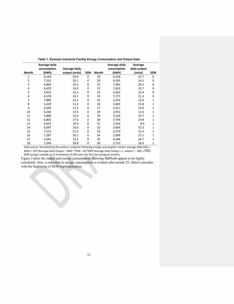
31

Table 1. Example Industrial Facility Energy Consumption and Output Data

Month

Average daily consumption

(kWh) Average daily output (units) SEM Month

Average daily consumption

(kWh)

Average daily output

(units) SEM 1 8,164 23.9 0 19 6,318 15.7 0 2 7,352 20.1 0 20 6,505 14.5 0 3 6,869 19.2 0 21 7,481 20.2 0 4 6,429 16.0 0 22 7,653 23.7 0 5 5,815 13.2 0 23 6,422 15.4 0 6 6,578 18.1 0 24 7,271 21.3 0 7 7,889 23.3 0 25 5,201 12.0 1 8 5,439 11.6 0 26 5,669 21.8 1 9 6,049 11.5 0 27 4,312 19.9 1

10 6,266 13.5 0 28 2,951 11.6 1 11 5,898 12.0 0 29 3,520 19.7 1 12 6,801 17.6 0 30 4,704 24.8 1 13 6,654 19.4 0 31 2,416 8.6 1 14 6,097 14.0 0 32 3,669 15.3 1 15 7,215 21.5 0 33 3,270 15.3 1 16 7,387 20.1 0 34 3,909 21.1 1 17 5,641 13.2 0 35 4,584 24.7 1 18 7,394 20.8 0 36 3,710 18.4 1

Data source: Simulated by the authors using the following energy consumption model: average daily kWh = 4010 + 155*Average Daily Output – 2005 * SEM – 62*SEM*Average Daily Output + ε, where ε ∼ N(0, √200). SEM savings ramped up in increments of 25% over the first four program months.

Figure 2 plots the output and energy consumption, showing that both appear to be highly correlated. Also, a reduction in energy consumption is evident after month 25, which coincides with the beginning of SEM implementation.

32

Figure 2. Plot of SEM Facility Electricity Consumption and Output vs. Time

Suppose that, using the model-selection methods described in Section 3 of this protocol, the evaluator posits the following regression model of facility kWh during the baseline period:

kWht = β0 + β1yt + εt (Equation 3)

Where:

kWht = Facility average daily electricity consumption in month t.

β0 = Constant term to be estimated, indicating average daily electricity consumption unrelated to the facility output.

β1 = Coefficient to be estimated, indicating the effect of an additional unit of output on electricity consumption.

yt = Facility average daily output in month t.

εt = Error term.

The evaluator estimates the model using the first 24 monthly observations from the baseline period data.

Table 2 shows results from the OLS estimation of Equation 3. The model coefficients are estimated precisely—each is statistically significant at the 1% level—and have the expected signs. The coefficient on average daily output indicates average energy consumption increased by an average of 176 kWh for each unit of output.

33

Table 2. Estimates of Facility Forecast Regression Model

Dependent Variable Average Daily kWh

Intercept 3653* (214.4)

Average daily output 176.1* (12.0)

Regression Standard Error 229.06 F statistic 216.7 R2 0.908 N 24 Notes: Model estimated by OLS. Standard errors in parentheses. * Denotes statistically significant at the 1% level.

Next, using the regression results, the evaluator estimates the adjusted baseline for each month of the reporting period. Monthly adjusted baseline electricity consumption (kWh) equals (3653 + 176*average daily output during the month) times the number of days in the month.

Table 3 shows the calculation of the monthly adjusted baseline and SEM savings. Monthly SEM savings were estimated as the difference between the adjusted baseline and metered energy consumption.

Table 3. Estimates of Facility Adjusted Baseline Energy Consumption and Savings

SEM reporting

period month

Average daily

output (units)

Metered average daily consumption

(kWh)

Adjusted baseline average daily consumption

(kWh) Days

SEM monthly savings

Cumulative SEM savings

to date 25 12.0 5,201 5,772 31 17,698 17,698 26 21.8 5,669 7,499 28 51,235 68,933 27 19.9 4,312 7,152 31 88,059 156,992 28 11.6 2,951 5,693 30 82,264 239,257 29 19.7 3,520 7,121 31 111,640 350,897 30 24.8 4,704 8,023 30 99,573 450,470 31 8.6 2,416 5,175 31 85,524 535,994 32 15.3 3,669 6,343 31 82,884 618,878 33 15.3 3,270 6,338 30 92,041 710,919 34 21.1 3,909 7,377 31 107,480 818,399 35 24.7 4,584 7,994 30 102,291 920,690 36 18.4 3,710 6,891 31 98,608 1,019,298

Notes: For description of calculations, see text. - Lastly, the evaluator estimates savings for the first SEM program year by summing the monthly SEM savings for the first 12 reporting period months.

The last column of Table 3 shows the cumulative savings to date. By the end of the first year, it is estimated that the program had saved approximately 1,019,000 kWh. Based on

Formatted: Centered

Formatted: Centered

Formatted: Centered

Formatted: Centered

Formatted: Centered

Formatted: Centered

Deleted: Monthly

Deleted: Reference average daily

Deleted: program

34

implementation of Equation 2, the standard error of the savings estimate is 17,646 kWh, and the estimated 95% confidence interval for the SEM savings is [984,710 kWh, 1,053,885 kWh].

4.1.2 Pre-Post Models An alternative to the forecast approach is to use baseline period and reporting period data to estimate the facility average energy savings per time interval as a parameter of the regression model. This pre-post modeling approach estimates a modified version of Equation 1, with additional variable(s) to indicate the occurrence of SEM activity:

et = β0 + β1 x1t + β2 x2t + … + βk xkt + θdt + εt (Equation 4)

Where:

dt = An indicator variable for SEM activity at the facility. It equals one if the facility initiated SEM in the current or in a previous interval; it equals zero otherwise.

θ = A coefficient to indicate the average effect per time interval of SEM activity on facility energy consumption.

The main differences between this model and the forecast model are that the pre-post model is estimated using both baseline period and reporting period data. The pre-post model also includes an indicator variable dt to signify SEM program activity. A third difference is that the forecast model does not make any assumptions about how savings depend on the model explanatory variables. In contrast, savings are assumed to have a “level effect” on energy consumption for this pre-post model. Since dt enters the model without being interacted with any other variables, savings do not depend on any of the independent variables in Equation 4.

Energy savings equal the product of the facility average savings per time interval and the number of time intervals during the reporting period:

S = θTP

If 𝜃𝜃� is the estimate of θ, then the variance of the estimated savings �̂�𝑆 equals:

var(�̂�𝑆)= var(𝜃𝜃�) (TP)2

4.1.2.1 Estimating SEM Savings in Multiple Sub-Periods Evaluators may want to estimate savings for multiple periods to obtain savings estimates for different program years or to track growth, persistence, or decay of savings over time. To estimate SEM savings in multiple reporting periods, the evaluator can add more SEM reporting-period indicator variables to the regression, as follows:

et = β0 + β1 x1t + β2 x2t + … + βk xkt + ∑ 𝐽𝐽𝑗𝑗=1 θjdjt + εt (Equation 5)

Where:

Deleted: ¶

Deleted: ,

35

dj,t = An indicator for SEM activity in sub-period j, j = 1, 2, …, J, of the reporting period. This variable equals one if time interval t is in the jth sub-period and the facility implemented SEM in the current interval or a previous interval; it equals zero otherwise.

θj = A coefficient indicating SEM average energy savings per interval during the jth sub-period. The interval savings are measured relative to the baseline period.

As an objective of SEM programs is continuous improvement of energy efficiency, evaluators may want to measure year-over-year changes in savings. Evaluators can use Equation 5 to measure these changes. Suppose that the time intervals are days and dj,t is an indicator variable for the jth program year. Then the incremental annual energy savings between the second and third program years would be calculated as follows:

Incremental annual savingsYr2,Yr3 = 365*(θ3 - θ2)

The incremental annual savings between other program years can be estimated analogously.

4.1.2.2 Estimating SEM Savings as a Function of Output or Weather Equation 3 assumes that SEM resulted in a level-shift in facility energy consumption. In other words, SEM’s impact did not depend on output, weather, occupancy, or other variables affecting the facility’s energy consumption. This might be a reasonable assumption for facilities where savings from SEM improvements did not vary closely with output or other variables. For example, a facility undertaking a lighting retrofit might have savings that do not vary with the facility’s output. In many facilities, however, SEM savings will be closely correlated with output or other observed drivers of energy consumption. such as occupancy. In this case, the evaluator can model SEM savings as a function of the model independent variables:

et = β0 + β1 x1t + β2 x2t + … + βk xkt + θdt + θk dt * xkt + εt (Equation 6)

Where all variables are defined as before, except:

θk = A coefficient indicating the SEM average energy savings, per time interval, per unit change of variable xk.

In this specification, SEM can have a level savings effect, indicated by θ, as well as a slope-shift savings effect that depends on the variable xk. For example, if variable xk is facility output, then θk is the SEM savings per unit of output.

Energy savings during the reporting period would equal the following:

S = θTP + θk∑ 𝑥𝑥𝑘𝑘,𝑡𝑡𝑇𝑇𝑃𝑃𝑡𝑡=1

4.1.2.3 Example of Pre-Post Regression Model Savings Estimation This section illustrates a pre-post regression savings estimation, using data for all 36 intervals from the baseline and reporting periods in Table 1.

Deleted: ,

Deleted: Example

Deleted: from

Deleted:

Deleted: the above example of a forecast regression savings estimation…

36

Again, the evaluator wishes to estimate savings for the first SEM program year, thus specifying the following pre-post model:

kWht = β0 + β1yt + θdt + θ1yt*dt + εt (Equation 7)

Where:

kWht = Facility average daily energy consumption in month t.

β0 = Coefficient to be estimated, indicating facility average daily electricity consumption during the baseline period.

β1 = Coefficient to be estimated, indicating average facility electricity consumption per unit of output.

yt = Facility average daily production output during month t.

θ = Coefficient to be estimated, indicating SEM average electricity savings per day for the facility’s baseload. These are savings from energy consumption that do not vary with the amount of output.

dt = Indicator variable for SEM program activity. This variable equals one if SEM was implemented in the current month or in a previous month; it equals zero otherwise.

θ1 = Coefficient to be estimated, indicating SEM average electricity savings per unit of output.

εt = Model error.

This specification includes an indicator variable for SEM activity as well as for the SEM indicator interacted with output. The evaluator includes both variables, in expectation that SEM has both level and per-unit-of-output effects on facility energy consumption.

Table 4 shows estimates of the coefficients presented in Equation 7. The first column shows estimates of the coefficients in Equation 7. The second column shows estimates of Equation 7 without the interaction variable between the SEM indicator and output (to demonstrate the effect on estimated savings of mis-specifying the energy consumption model).

Table 4. Pre-Post Regression Model Estimates

Dependent Variable Pre-Post Model 1 Average daily kWh

Pre-Post Model 2 Average daily kWh

Intercept 3,652.9*** (454.3)

4,208.2*** (355.9)

Average daily output 176.1*** (25.3)

144.3*** (19.5)

SEM -1,536.2** -2,779.8***

Deleted: Facility Energy Consumption

37

(688.1) (178.0) SEM*Average daily consumption

-70.5* (37.8)

F statistic 105.8 146.0 R2 0.908 0.898 N 36 36 Notes: Output based on analysis of data in Table 1. Model estimated by OLS. Standard errors in parentheses. *, **, *** denotes statistically significance at the 1%, 5%, and 10% levels, respectively.

According to Model 1, SEM reduced energy consumption by an average of about 1,536 kWh per day, plus approximately 71 kWh per unit of output. The SEM program coefficients were statistically significant at the 5% and 1% levels, respectively. Since output averaged 17.8 units per day across the reporting period, the SEM program averaged savings of 2,790 kWh per day (=17.8*70.5 + 1,536.2).

Though the second model was mis-specified because it omitted the interaction between the SEM indicator variable and output, the second model yielded an estimate of savings very similar to that of the correctly-specified Model 1. According to Model 2, daily savings from SEM averaged 2,780 kWh. Nevertheless, Model 1 has the advantage of allowing electricity savings to be decomposed into baseload savings and savings per unit of output and therefore may yield more useful information to the evaluator or program implementer.

The evaluator can then use the pre-post regression model to obtain an estimate of SEM program annual savings. Using the results of Model 1, the evaluator estimates annual savings as the sum of energy savings from baseload and production energy consumption:

Annual SEM savings = days*1536.2 kWh/day + annual output*70.5 kWh/unit of output

Assuming that the facility operated 365 days and that annual output equaled 6,467 units, annual SEM energy savings equaled 1,016,576 kWh. The estimated 95% confidence interval equaled [893,745 kWh, 1,139,407 kWh].35

These estimates can be compared to an annual savings estimate from the forecast Model 1 of 1,019,298 kWh. The pre-post Model 1 and Model 2 yielded estimates of annual savings of 1,016,576 kWh and 1,014,608 kWh, respectively.

4.1.3 Comparison of Forecast and Pre-Post Approaches The forecast and pre-post models take different approaches to estimating savings. The forecast approach fits a model using data from the baseline period and then uses that model to predict

35 The confidence interval requires accounting for the co-variance between the estimated coefficients on SEM and SEM*Average daily consumption. The evaluator can calculate the confidence interval by outputting the variance-covariance matrix or by using statistical software such as SAS, STATA, or R.

Deleted:

Deleted: .

38

energy consumption in the reporting period. The pre-post approach fits one model with SEM level-shift or slope-shift indicator variables using data for the baseline and reporting periods.

Despite these differences, the forecast and pre-post models are expected to yield similar estimates of the adjusted baseline and SEM savings. This was illustrated in the preceding comparison of the forecast and pre-post model savings estimation examples. The equivalence of the two approaches is analyzed from a conceptual perspective in the this protocol’s Appendix (section 7). The models yielded the same predictions of the adjusted baseline, shown by identical intercepts and coefficients on average daily output for the two models. The models also yielded very similar savings estimates.

In general, as this document’s appendix demonstrates, the forecast and pre-post models will produce unbiased savings estimates if the following conditions hold:

(1) The pre-post model is specified as if SEM affects all energy consumption relationships modeled during the baseline period. Any variable expected to affect baseline period energy consumption should be interacted with an indicator variable for SEM and included in the regression.

In the above example, the pre-post model includes both an intercept for the reporting period (the SEM level shift) and an interaction between output and SEM (the SEM slope shift), thereby allowing baseload energy consumption and energy consumption per unit of output to differ between the baseline and reporting periods:

(2) The forecast and pre-post models are correctly specified in the sense that the energy consumption regression models closely approximate the facility’s true energy consumption relationships during the baseline period. The models do not omit variables that were correlated with SEM implementation and facility energy consumption.

In this protocol’s examples, the true energy consumption relationships are known because the data are simulated. In general, however, the evaluator will not know the true facility energy consumption model, and the forecast and pre-post models may produce biased savings estimates. To obtain a valid savings estimate, the evaluator should collect facility data and to build a valid model of facility energy consumption. Section 3 of this protocol describes the data collection and model specification processes for SEM evaluation.

4.1.4 Normalized Operating Conditions Models The forecast and pre-post models produce estimates of SEM energy savings for the reporting period. The savings reflect the facility’s operating conditions during the reporting period. However, operating conditions during the reporting period may have been atypical, producing savings that the facility may not expect in most years. Instead, evaluators may want an estimate of annual savings for the facility under normal operating conditions, which might be characterized by particular expected weather, occupancy levels, or production.

Suppose that facility energy consumption for interval t of the baseline period, et, can be modeled as:

Deleted: demonstrated

Deleted: make sufficient effort to

Formatted: NREL_Head_03_Numbered

Formatted: NREL_Body_Text, Left, Space After: 0 pt, Nobullets or numbering

39

et = β0 + β1xt + εt (Equation 8)

and suppose that the facility’s energy consumption for interval t of the reporting period, etP, can be modeled as:

etP = β0

P + β1Pxt

P + εtP (Equation 9)

where P denotes the reporting period and xt is units of facility output, a weather-related variable, or occupancy. The beta coefficients, β0 and β1, indicate, respectively, the facility’s baseload consumption per interval and the marginal effect of xt on energy consumption. The beta coefficients for the reporting period, β0

P and β1

P, reflect any SEM impacts.

Furthermore, suppose that 𝑥𝑥𝑘𝑘𝑁𝑁 is the normal or expected value of x for interval k, k=1, 2, …, K, of the calendar year. For example, x could be heating degrees, and 𝑥𝑥1𝑁𝑁, 𝑥𝑥2𝑁𝑁, …, 𝑥𝑥𝐾𝐾𝑁𝑁 would be expected values of heating degrees for intervals (e.g., days, weeks, or months) of the calendar year.

Evaluators can obtain an estimate of SEM savings under normal operating conditions by following these steps:

(1) Estimate Equation 8, the facility consumption model for the baseline period, using baseline period data, and Equation 9, the facility consumption model for the reporting period, using reporting period data.

(2) Predict energy consumption under normal operating conditions for the baseline period and reporting period using estimates from step 1 to obtain the normalized adjusted consumption for each interval k of the calendar year:

𝑒𝑒 𝑘𝑘𝑁𝑁� = b0 + b1 𝑥𝑥𝑘𝑘𝑁𝑁 (Equation 10)

𝑒𝑒 𝑘𝑘𝑁𝑁,𝑃𝑃�= 𝑏𝑏0𝑃𝑃 + 𝑏𝑏1𝑃𝑃 𝑥𝑥𝑘𝑘𝑁𝑁 (Equation 11)

(3) Estimate annualized energy savings under normal operating conditions, SN, as the difference between normalized adjusted consumption for the baseline period and the normalized adjusted consumption for the reporting period.

SN = ∑ 𝑒𝑒 𝑘𝑘𝑁𝑁� − ∑ 𝑒𝑒 𝑘𝑘𝑁𝑁,𝑃𝑃�𝐾𝐾

𝑘𝑘=1 𝐾𝐾𝑘𝑘=1 (Equation 12)

4.1.4.1 Example of Normalized Operating Conditions Savings Estimation In Table 1, the industrial facility produced 6,497 units of output during the 12 months of the reporting period. Suppose that this output was abnormally low and that the facility usually produces 10,000 units of output annually. How much electricity would the facility save under normal operating conditions?

First, the evaluator would estimate the facility’s electricity consumption during a normal year before implementation of SEM. This can be calculated with the forecast model coefficients in Table 2. The facility would have consumed 3,094,345 kWh during a normal year before

Formatted: NREL_Body_Text, Space After: 0 pt, No bulletsor numbering



Formatted: NREL_Body_Text, Space After: 0 pt, No bulletsor numbering



Formatted: Indent: Left: 0.5", First line: 0.5", No bulletsor numbering

Formatted: NREL_Body_Text, Left, Space After: 0 pt

Formatted: Superscript


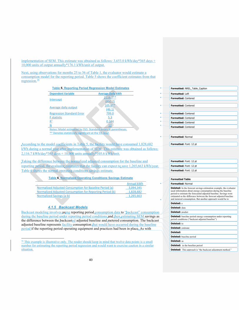
40

implementation of SEM. This estimate was obtained as follows: 3,653.0 kWh/day*365 days + 10,000 units of output annually*176.1 kWh/unit of output.

Next, using observations for months 25 to 36 of Table 1, the evaluator would estimate a consumption model for the reporting period. Table 5 shows the coefficient estimates from that regression.36

Table 5. Reporting Period Regression Model Estimates

Dependent Variable Average Daily kWh

Intercept 2116.7** (850.7)

Average daily output 105.6** (46.1)

Regression Standard Error 799.0 F statistic 5.3 R2 0.344 N 12 Notes: Model estimated by OLS. Standard errors in parentheses. ** Denotes statistically significant at the 5% level.

According to the model coefficients in Table 5, the facility would have consumed 1,828,682 kWh during a normal year after implementation of SEM. This estimate was obtained as follows: 2,116.7 kWh/day*365 days + 10,000 units annually*105.6 kWh/unit.

Taking the difference between the normalized adjusted consumption for the baseline and reporting period, the evaluator estimates that the facility can expect to save 1,265,663 kWh/year. Table 6 shows the normal operating conditions savings estimate.

Table 6. Normalized Operating Conditions Savings Estimate

Annual kWh Normalized Adjusted Consumption for Baseline Period (a) 3,094,345 Normalized Adjusted Consumption for Reporting Period (b) 1,828,682 Normalized Savings (a-b) 1,265,663

4.1.5 Backcast Models Backcast modeling involves using reporting period consumption data to “backcast” consumption during the baseline period under reporting period conditions and then estimating SEM savings as the difference between the backcasted adjusted baseline and metered consumption. The backcast adjusted baseline represents facility consumption that would have occurred during the baseline period if the reporting period operating equipment and practices had been in place. As with

36 This example is illustrative only. The reader should keep in mind that twelve data points is a small number for estimating the reporting period regression and would want to exercise caution in a similar situation.

Formatted: NREL_Table_Caption

Formatted: Left

Formatted: Centered

Formatted: Centered

Formatted: Centered

Formatted: Centered

Formatted: Centered

Formatted: Centered

Formatted: Normal





Formatted Table

Formatted: NormalDeleted: In the forecast savings estimation example, the evaluator used information about energy consumption during the baseline period to estimate the forecasted adjusted baseline. Savings were estimated as the difference between the forecast adjusted baseline and metered consumption. But another approach would be to

Deleted: e

Deleted: data

Deleted: predict

Deleted: baseline period energy consumption under reporting period conditions (“backcast adjusted baseline”)

Deleted: to

Deleted: estimate

Deleted:

Deleted: baseline period

Deleted: as

Deleted: in the baseline period

Deleted: This approach is “the backcast adjustment method.”

41

forecast method, this method requires the development of a model that characterizes energy consumption as a function of relevant variables.

Evaluators may find the backcast approach useful when:

• Evaluators have limited data on energy consumption and corresponding independent variables during the baseline period but detailed data for the reporting period.

• Facility operating conditions during the reporting period are inclusive of facility operating conditions during the baseline period conditions, but not vice-versa.

For example, an industrial facility may have produced only low levels of output during the baseline period but low and high levels during the reporting period. A forecast model may produce an inaccurate estimate of adjusted baseline consumption because some reporting period conditions (i.e., high output levels) were outside of those experienced during the baseline. In contrast, the backcast adjustment approach is expected to yield valid predictions of baseline period energy consumption because the reporting period included low levels of output.

Evaluators should apply the backcast approach judiciously, considering whether the approach yields the desired savings estimate. Typically, evaluators will want an estimate of savings for the reporting period or for standard operating conditions. However, the backcast approach yields an estimate of counterfactual savings, what SEM energy savings would have been during the baseline period. If the facility’s operating conditions differ substantially between the baseline and reporting periods, the backcast approach may not produce the desired estimate.

4.1.5.1 Example of Backcast Savings Estimation Suppose an evaluator wanted to apply the backcast approach to the facility consumption data in Table 1. The evaluator first estimates a regression model of facility consumption using reporting period data for months 25-36. Table 5 shows results of that regression.

Next, the evaluator would use the regression coefficients in Table 5 to backcast the facility’s consumption during the baseline period. Table 6 shows the facility would have consumed 1,414,907 kWh and 1,479,539 kWh during, respectively, months 1-12 and months 13-24 of the baseline period if it had implemented SEM.

The evaluator would then compare the backcasted adjusted baseline consumption with the metered consumption to estimate the backcast savings for the two baseline periods. Table 7 presents the backcast estimates.

Table 7. Backcast Model Savings Estimates

Months (1-12) Months (13-24) Baseline Period Consumption (kWh) 2,419,031 2,496,205 Backcast Adjusted Baseline Consumption (kWh) 1,414,907 1,479,539 Backcast Electricity Savings Estimate (kWh) 1,004,125 1,016,666

Deleted: describing

Deleted: , but in this case for the reporting period

Deleted: It results in an estimate of backcasted SEM savings, what savings would have been if SEM had been implemented during the baseline period.…A A

Deleted: A

Deleted: adjustment method

Deleted: may be

Deleted: when e

Formatted: Bulleted + Level: 1 + Aligned at: 0.25" +Indent at: 0.5"

Deleted: energy consumption and relevant variables for

Deleted: It is also useful when f

Deleted: It may be inappropriate for the evaluator to use data from the baseline period to build a regression model to predict the

Deleted: Facility operating conditions and energy consumption may have been very different at low and high output levels. In this case, the evaluator could use reporting period data to build a model to predict what energy consumption would have been during the baseline period if SEM had been implemented. The evaluator would then compare baseline period metered energy consumption with the backcast adjusted baseline. T

Deleted: model

Moved down [3]: ¶Evaluators should recognize that facility operating conditions during the baseline and reporting periods may differ, in which case savings estimated for the baseline period and savings estimated for reporting period conditions will differ. Therefore, e

Moved down [3]: ¶Evaluators should recognize that facility operating conditions during the baseline and reporting periods may differ, in which case savings estimated for the baseline period and savings estimated for reporting period conditions will differ. Therefore, e

Deleted: carefully

Deleted: conditions

Deleted: an estimate of savings for expected or typical

Moved (insertion) [3]Deleted: Evaluators should recognize that

Moved (insertion) [3]

Deleted:

Deleted: during


Formatted: NREL_Table_Caption

Formatted Table

42

Again, the evaluator should keep in mind that the backcast savings are estimates of counterfactual SEM savings during the baseline period and may not equal the actual savings that the program achieved during the reporting period. In this example, the backcast model produced annual savings estimates that were very close to the forecast model estimate of annual savings (1,019,000 kWh) because annual output levels during the baseline and reporting period were approximately equal. If output levels had differed, the forecast model and backcast model savings estimates would have been differed too.

4.1.6 Panel Regression Models To this point, the protocol has emphasized analysis of individual facilities because many program administrators require an SEM savings estimate for each facility. Also, many industrial and large commercial facilities have unique characteristics that make group analysis problematic. For example, food processors, lumber mills, hospitals, and wastewater treatment facilities have very different outputs, production processes, and energy consumption characteristics. These differences make regression modeling for groups of very different facilities difficult.

There are, however, circumstances when group or panel analysis of energy consumption for a group of facilities may be appropriate. A panel consists of data for two or more facilities and multiple observations for each sampled facility. A panel data set should cover the baseline and reporting periods. Panel regression analysis yields an estimate of the average savings per facility, per unit of time; this can provide a more economical means of program impact evaluation than estimating savings for each site.

Panel analysis is appropriate when the evaluator does not require facility-specific savings and when program populations or subpopulations have similar energy consumption characteristics. For example, group analysis could be used to estimate SEM program average savings per facility for a population of office buildings or primary or secondary schools. These types of buildings have relatively similar energy end uses (lighting and space conditioning) and energy consumption intensities. This analysis also may be appropriate for an SEM program targeting a specific industrial sector, such as food processing.

Suppose the evaluator has data on baseline and reporting period energy consumption and energy consumption drivers for i=1, 2, …, N facilities.37 Then a panel regression of facility i energy consumption during time interval t would be:

eit = β1 x1it + β2 x2it + … + βk xkit + θdit + αi + εit (Equation 13)

where all of the variables affecting energy consumption of a facility have been indexed by k, k=1,2, …, k, and the other variables are defined as before; i indexes the facility, and t indexes the time period.

37 This panel regression approach assumes that reference energy use was estimated using pre-SEM engagement facility energy use of SEM participants. An alternative approach for estimating reference energy use would be to identify a comparison group of nonparticipant facilities and to use their energy use during the SEM performance period as a baseline. See Agnew (2013) for baseline approaches employing a control group.

Deleted: Analysis

Deleted: regression

Deleted: SEM

Deleted: y energy consumption

Deleted: most

Deleted: many

Deleted: energy consumption and production

Deleted:

Deleted: .

Deleted: are an important reason for evaluators of most ratepayer-funded programs to conduct individual energy consumption analysis for each site

Deleted: panel regression

Deleted: facility

Deleted: for estimating SEM program savings

Deleted: This type of analysis is appropriate when the evaluator does not require facility-specific savings and when program populations or subpopulations have similar energy consumption characteristics. For example, panel regression analysis could be used to estimate SEM program average savings per facility for a population of office buildings or primary or secondary schools. These types of buildings have relatively similar energy end uses (lighting and space conditioning) and energy consumption intensities. Panel regression analysis also may be appropriate for an SEM program targeting a specific industrial sector, such as food processing.¶

Deleted: P

Deleted: data

Deleted: energy consumption

Deleted: sites

Deleted: 8

Deleted: Where



43

For example, x1it is the variable x1 (e.g., outside temperature) for facility i during time interval t, and αi is the error term specific to facility i that does not vary over time.38 Instead of using energy consumption as the dependent variable, evaluators may want to normalize the dependent variable by dividing it by the number of square feet or the number of units of output to account for differences between facilities in floor area or other variables affecting energy consumption.

The term αi may or may not be correlated with the x variables and dit. An evaluator who believes αi is correlated should estimate a fixed effects model, which involves estimating Equation 8 by OLS, with a separate intercept for each facility in the analysis sample. The facility intercepts control for all unobservable, time-invariant factors specific to the facility that may be correlated with the other variables in the model.

Alternatively, an evaluator who believes αi is uncorrelated with the independent variables should estimate a random effects model, which involves estimating Equation 8 by generalized least squares, first by estimating the covariance matrix of the error term, and then using the estimated covariance matrix in a second-stage estimation of the Equation 8.

In general, when there is a choice between the two estimation methods, fixed effects estimation is recommended because it yields consistent estimates of the model parameters when the assumptions of the random effects model or the fixed effects model hold true (Greene 2012). The random effects estimator, however, is not consistent when the assumptions of the fixed effects model hold true.

Estimation of Equation 8 yields an estimate of the average program effect θ. With the panel regression model, program savings can be estimated as shown:

S = θ ∑ ∑ 𝑑𝑑𝑖𝑖,𝑡𝑡𝑇𝑇𝑃𝑃𝑡𝑡=1

𝑁𝑁𝑖𝑖=1

The program savings are the product of the average savings per facility, per interval and the total number of facility SEM engagement intervals during the reporting period.

While panel regression analysis does not yield a savings estimate for each facility, it can be used to estimate how program effects depend on the preexisting characteristics of participants. For example, the model can be used to estimate savings as a function of floor area or by school type (e.g., elementary, secondary). Evaluators can do this by interacting indicators for program activity with participant characteristic variables.

38 The regression specification excludes time interval fixed effects, which would capture impacts of each time interval on average facility energy use. If there is no variation between facilities in the data of first SEM implementation, the evaluator will be unable to include both time interval fixed effects and an SEM indicator variable because the SEM indicator variable and the fixed effects will be co-linear. If the regression includes interaction variables between the SEM indicator and other variables but not an SEM indicator, the evaluator could include time interval fixed effects in the regression. If the number of facilities is sufficiently large and there is enough variation between facilities in the date of first SEM implementation, the evaluator can include time interval fixed effects.



44

4.2 Non-Routine Adjustments Evaluators may need to make non-routine adjustments to improve the accuracy of the adjusted baseline. A non-routine adjustment refers to a one-time, ad hoc adjustment to the adjusted baseline to account for a change in facility energy consumption that cannot be modeled econometrically. Not accounting for such changes may bias the savings estimate. Evaluators, however, should make these adjustments sparingly and objectively, without regard to the expected effect on the savings estimate.

For example, suppose that an industrial facility replaced equipment and implemented SEM at the same time. The equipment replacement was scheduled far in advance of SEM implementation, but both had the effect of reducing energy consumption per unit of output. Since the equipment replacement and SEM implementation coincided, the evaluator may not be able to use regression analysis to identify the SEM savings.

In such instances, if an engineering-based estimate of the change in energy consumption is available, the evaluator can adjust the adjusted baseline consumption to account for the equipment change. The difference between the regression and non-routine adjusted baseline and metered energy consumption would then yield an estimate of the SEM savings. If an estimate of the impact of the change in energy consumption is not available, it may not be feasible to use statistical methods to estimate the SEM savings.

Non-routine adjustments of this type should be used sparingly. The evaluator should first attempt to account for the change in energy consumption in the regression model. In the above example, if the equipment replacement had been a more efficient space conditioning system and SEM energy savings did not depend on weather, the evaluator might be able to use regression to control for the equipment replacement by modeling energy consumption as a function of heating degree days (HDDs), cooling degree days (CDDs), and the date of the equipment change.

When non-routine adjustments must be made, evaluators should apply them based on careful engineering analysis, precisely documenting all assumptions and calculations. The evaluator should carefully review the assumptions and accuracy of the calculations.

4.3 Site Data Collection Thus far, this protocol has assumed that evaluators would not perform primary data collection. Evaluators would analyze data on facility energy consumption, output, and weather collected from program implementers, the utility, or third-party data providers. The exception would be conducting interviews with facility staff or program implementers to gather additional information about the facility’s energy consumption and implementation of SEM. Such primary data collection can greatly improve evaluators’ understanding of facility energy consumption, and this protocol highly recommends conducting these interviews.

In some circumstances, however, evaluators may be able to significantly improve the accuracy of SEM savings estimates by conducting on-site facility inspections and data collection. Many SEM program facilities install capital equipment or retrofit measures as a result of SEM engagement. Other facilities may have installed capital measures during the baseline period.

Deleted: to estimate savings

Deleted: energy

45

Evaluators can use site visits to improve the accuracy of capital project savings estimates needed for developing a baseline model or estimating SEM savings. Specifically, site visits can be used to verify key assumptions in the calculation of capital project savings. Evaluators also can use site visits to check the reasonableness of SEM savings estimates obtained from statistical models.

More specifically, this protocol recommends evaluators consider conducting site visits when one or more of the following conditions hold true:

• An evaluation objective is to obtain separate estimates of SEM capital measure savings and SEM operations, maintenance, and behavioral savings;

• Savings from capital measures constitute a large share of SEM savings, and the statistical analysis yields an SEM savings estimate with substantial uncertainty; or

• It is necessary to perform a one-time, non-routine adjustment to the baseline or reporting-period energy consumption to account for capital measure savings or for a change in facility operations, and a site visit can significantly reduce uncertainty about the magnitude of such adjustments.

When one or more of these conditions hold, an on-site measurement and verification that better characterizes the impacts of such changes on facility energy consumption may improve the accuracy of the SEM savings estimates.

This protocol recommends that evaluators follow IPMVP (2012), which recommends best practices for conducting on-site data collection for the evaluation of capital measure and retrofit projects. For capital equipment and retrofit measures installed as part of SEM engagement the most appropriate evaluation options are as follows:

• Operational Verification. For this type of savings estimation method, the evaluator relies on a variety of on-site data collection activities (e.g., visual inspections, spot measurements, data trending reviews) to verify that an energy efficiency measure is installed and functioning as intended.

• IPMVP Option A, Retrofit Isolation: Key Parameter Measurement. For this method, the evaluator uses engineering calculations and partial site measurements to verify the savings resulting from specific measures. The evaluator estimates some parameters that are not measured.

• IPMVP Option B, Retrofit Isolation: All Parameter Measurement. For this method, the evaluator uses engineering calculations and ongoing site measurements to verify savings as the change in energy consumption of the affected system. This may be appropriate for variable frequency drives, where the evaluator could use long-term metering to determine the true reduction in motor energy over various seasonal and loading cycles.

Evaluators should know that IPMVP Option A and Option B typically require baseline-period and reporting-period data, and that baseline-period data may be unavailable if not previously collected.

When selecting an on-site data gathering approach, the evaluator should seek to balance the expected reduction in uncertainty with the project’s resources and budget. To decrease the

46

uncertainty of estimates, the evaluator should measure and meter where experience has shown that energy consumption can vary widely. The evaluator also should measure and meter in situations where existing estimates of capital project savings remain uncertain. Through this approach, the evaluator can confirm that the reported capital and retrofit measures are (1) installed, (2) functioning, and (3) operating appropriately. If the evaluator determines that the results from an installed measure differ from the assumptions expected in the approach, additional data may be collected to further evaluate the energy savings.

5 Other Evaluation Issues 5.1 Sampling Some SEM programs may enroll a large number of facilities, but they have evaluation budgets too small to support an impact evaluation of the population of facilities. In this case, the evaluator may need to analyze a random sample of facilities from the program population.

Evaluators can consult well-known guidelines and protocols for simple random sampling, stratified random sampling, and other, more complex sampling designs for efficiency program populations. Evaluators can find useful sampling guidelines in UMP Chapter 11: Sample Design Cross-Cutting Protocols (NREL 2013). Sampling Techniques (Cochran 1977) provides another good reference.

5.2 Free-ridership, Spillover, and Net Savings This protocol is primarily concerned with estimation of SEM program gross savings using a regression-adjusted baseline. The issues and approach for estimating SEM net savings are very similar to those for other ratepayer-funded, energy efficiency measures. This protocol recommends that evaluators consult UMP Chapter 23: Estimating Net Savings: Common Practices (NREL 2014) for guidance.

47

6 References Agnew, K.; Goldberg, M. (April 2013). Chapter 8: Whole-Building Retrofit with Consumption Data Analysis Evaluation Protocol. The Uniform Methods Project: Methods for Determining Energy Efficiency Savings for Specific Measures. NREL.

Amundson, T., et al. (2013). “Elements of Defensible Regression-Based Energy Models for Monitoring and Reporting Energy Savings in Industrial Energy Efficiency Operation and Maintenance Projects.” Paper presented at the 2013 ACEEE Summer Study on Energy Efficiency Industry.

ASHRAE. (2014). ASHRAE Guideline 14-2014—Measurement of Energy and Demand Savings. Atlanta, Ga.: American Society of Heating, Refrigerating and Air-Conditioning Engineers.

Bonneville Power Administration. (2012). Regression for M&V: Reference Guide. Prepared for BPA by Research into Action, Inc. et al. Available at: https://www.bpa.gov/EE/Policy/Imanual/Documents/July%20documents/3_BPA_MV_Regression_Reference_Guide_May2012_FINAL.pdf

Cadmus Group. (February 2013). Energy Smart Industrial—Energy Management Pilot Impact Evaluation. Prepared for Bonneville Power Administration. Available online: http://www.bpa.gov/EE/Utility/research-archive/Documents/BPA_Energy_Management_Impact_Evaluation_Final_Report_with_Cover.pdf

Cochran, W. G. (1977). Sampling Techniques. New York: John Wiley & Sons.

Consortium for Energy Efficiency. (2014a). CEE Strategic Energy Management Minimum Elements. Available at: https://library.cee1.org/content/cee-strategic-energy-management-minimum-elements/

Consortium for Energy Efficiency. (2014b). CEE Industrial Strategic Energy Management Initiative. Available at: http://library.cee1.org/sites/default/files/library/11282/Industrial_SEM_Initiative.pdf

Consortium for Energy Efficiency. (2015). SEM Program Case Studies Report. Available at: http://library.cee1.org/content/sem-program-case-studies-2014

Consortium for Energy Efficiency. (2016). Strategic Energy Management Initiative – 2015 CEE Annual Report. Available at: https://2015annualreport.cee1.org/initiatives/strategic-energy-management-initiative/

Deru, M. and P. Torcellini (2007). Source Energy and Emission Factors for Energy Use in Buildings. National Renewable Energy Laboratory Technical Report NREL/TP-550-38617. Available at http://www.nrel.gov/docs/fy07osti/38617.pdf.


Deleted: ¶

Deleted: .)

Deleted: .)

Deleted: .)

Deleted: .)

Deleted: .)

Deleted: .)

Deleted: .)

Deleted: .)

https://www.bpa.gov/EE/Policy/Imanual/Documents/July%20documents/3_BPA_MV_Regression_Reference_Guide_May2012_FINAL.pdf

https://www.bpa.gov/EE/Policy/Imanual/Documents/July%20documents/3_BPA_MV_Regression_Reference_Guide_May2012_FINAL.pdf

http://www.bpa.gov/EE/Utility/research-archive/Documents/BPA_Energy_Management_Impact_Evaluation_Final_Report_with_Cover.pdf



https://library.cee1.org/content/cee-strategic-energy-management-minimum-elements/

https://library.cee1.org/content/cee-strategic-energy-management-minimum-elements/

http://library.cee1.org/sites/default/files/library/11282/Industrial_SEM_Initiative.pdf

http://library.cee1.org/content/sem-program-case-studies-2014

https://2015annualreport.cee1.org/initiatives/strategic-energy-management-initiative/

https://2015annualreport.cee1.org/initiatives/strategic-energy-management-initiative/

48

DNV KEMA Energy and Sustainability; Research Into Action, Inc. (April 2014). NEEA Industrial Initiatives—Market Progress Evaluation Report #8. Prepared for the Northwest Energy Efficiency Alliance. Available online: http://neea.org/docs/default-source/reports/neea-industrial-initiatives–market-progress-evaluation-report-8.pdf?sfvrsn=10

Energy 350. (April 2014). Small to Medium Industrial SEM Energy Savings Validation. Prepared for the Northwest Energy Efficiency Alliance. Available online: http://neea.org/docs/default-source/reports/small-to-medium-industrial-sem-energy-savings-validation.pdf?sfvrsn=12

Energy Information Administration. (2008). Commercial Building Energy Consumption Survey, Table E1A, Major Fuel Consumption (Btu) by End Use for All Buildings (2003). Available at http://www.eia.gov/consumption/commercial/data/2003/pdf/e1a-e11a.pdf

Efficiency Valuation Organization. (2012). International Performance Measurement and Verification Protocol – Concepts and Options for Determining Energy and Water Savings Volume 1. Washington, D.C.: Efficiency Valuation Organization.

Frison, L.; Pocock, S.J. (1992). “Repeated Measures in Clinical Trial: Analysis Using Mean Summary Statistics and Its Implications from Design.” Statistics in Medicine 11: 1685-1704.

Greene, W. H. (2012). Econometric Analysis. 7th International Edition. Essex, England: Pearson Education.

Imbens, Guido and Donald M. Rubin (2015). Causal Inference for Statistics, Social, and Biomedical Sciences: An Introduction. New York: Cambridge University Press.

List, J.A., Sadoff, S.; Wagner, M. (2010). “So You Want to Run an Experiment, now What? Some Simple Rules of Thumb for Optimal Experimental Design.” National Bureau of Economic Research Paper 15701.

Khawaja, M. S.; Rushton, J.; Josh Keeling J. (April 2013). Chapter 11: Sample Design Cross-Cutting Protocols. The Uniform Methods Project: Methods for Determining Energy Efficiency Savings for Specific Measures. NREL.

Navigant Consulting, Inc. Impact Evaluation of Energy Trust of Oregon’s 2009–2011 Production Efficiency Program. December 2013. Prepared for the Energy Trust of Oregon. Available online: http://assets.energytrust.org/api/assets/reports/PE_Impact_Eval_2009-11.pdf

Northwest Industrial Strategic Energy Management Collaborative. (2013a). Tools and Methods for Addressing Auto-correlation in Energy Modeling. Available online: https://conduitnw.org/Pages/File.aspx?rid=1763

Northwest Industrial Strategic Energy Management Collaborative. (2013b). Tools and Methods for Addressing Multicollinearity in Energy Modeling. Available online: https://conduitnw.org/pages/file.aspx?rid=1762

Price, Phillip N. (2014). Review of Prior Commercial Building Energy Efficiency Retrofit Evaluation: A Report to Snohomish Public Utilities District. Ernest Orland Lawrence Berkeley

Deleted: .)

Deleted: .)

Deleted: .)

Deleted: .)

Deleted: .)

Deleted: .)

Deleted: .)

Deleted: .)

Formatted: Default Paragraph Font

http://neea.org/docs/default-source/reports/neea-industrial-initiatives--market-progress-evaluation-report-8.pdf?sfvrsn=10

http://neea.org/docs/default-source/reports/neea-industrial-initiatives--market-progress-evaluation-report-8.pdf?sfvrsn=10

http://neea.org/docs/default-source/reports/small-to-medium-industrial-sem-energy-savings-validation.pdf?sfvrsn=12

http://neea.org/docs/default-source/reports/small-to-medium-industrial-sem-energy-savings-validation.pdf?sfvrsn=12

http://www.eia.gov/consumption/commercial/data/2003/pdf/e1a-e11a.pdf

http://assets.energytrust.org/api/assets/reports/PE_Impact_Eval_2009-11.pdf

https://conduitnw.org/Pages/File.aspx?rid=1763

https://conduitnw.org/pages/file.aspx?rid=1762

49

National Laboratory. Available at: https://publications.lbl.gov/islandora/object/ir%3A1005583/datastream/PDF/view

Reddy, T. Agami and David E. Claridge, (2000). Uncertainty of ‘Measured’ Energy Savings from Statistical Baseline Models. HVAC & R Research: 6 (1), pp. 3-20.

Stern, F. (April 2013). Chapter 10. Peak Demand and Time Differentiated Energy Savings Cross Cutting Protocols. The Uniform Methods Project: Methods for Determining Energy Efficiency Savings for Specific Measures. NREL.

Thiel, Henri (1971). Principles of Econometrics. New York: John Wiley & Sons.

Violette D. M.; Rathburn, P. (September 2014). Chapter 23: Estimating Net Savings: Common Practices. The Uniform Methods Project: Methods for Determining Energy Efficiency Savings for Specific Measures. NREL.

U.S. Department of Energy (2017a). Qualified Energy Savings Measurement and Verification Protocol for Industry. Available at: [Link to be provided]

U.S. Department of Energy (2016b). Superior Energy Performance Certification Protocol for Industry. Available at: [Link to be provided]

U.S. Department of Energy (2017b). Superior Energy Performance Measurement and Verification Protocol for Industry. Available at: [Link to be provided]

Formatted: Default Paragraph Font

Deleted: .)

Deleted: .)

Formatted: Underline, Font color: Blue

Deleted: . 2012

Deleted: http://energy.gov/eere/amo/downloads/superior-energy-performance-measurement-and-verification-protocol-industry

Deleted: ¶

50

7 Appendix This appendix demonstrates the equivalence of the forecast savings and pre-post model approaches, showing that both produce unbiased savings estimates.

The appendix also derives the analytic formula for estimating the forecast savings standard error. The analytic formula captures two sources of uncertainty: the variance of the estimated baseline model coefficients; and the variance of metered energy consumption during the reporting period. It is necessary to account for both components to obtain an accurate estimate of the forecast savings standard error.

The first appendix section presents a model of facility energy consumption and defines SEM savings. The second section proves that, under the assumptions of the classical linear regression model, the pre-post and the forecast savings estimation methods yield unbiased estimates of SEM savings. The third section derives the formula for the forecast model standard error.

7.1 Definition of SEM Savings This section presents a general, or theoretical overview of calculating SEM savings. The formulas developed in 7.1 should not be used to actually calculate energy savings. Instead they are provided as reference to aid in demonstrating the equivalence of forecasting and pre-post modeling techniques in sections 7.2 and 7.3.

Suppose the following regression model describes facility electricity consumption in the baseline period:

kWht = α + βxt + εt (Equation A.1)

Where xt is an explanatory variable, such as output, and α and β are coefficients to be estimated. α can be interpreted as baseload energy consumption per interval, and β can be interpreted as the energy consumption per unit of output. The error term εt is normally, independently, and identically distributed with mean zero and variance σ2.

During the SEM reporting period, the facility implements changes to improve the efficiency of baseload energy consumption and energy consumption per unit of output. kWht

P is metered energy consumption during the baseline period. kWht

P can be expressed as the sum of the expected value of kWht

P, conditional on xtP plus an error: kWht

P = E[kWht | xtP, αP, βP] + εt

P. After implementation, facility electricity consumption during the SEM reporting period (P) is calculated as follows:

kWhtP = αP + βP

xtP + εt

P (Equation A.2)

Where P denotes reporting period, kWhtP and xt

P are energy consumption and output, and αP and βP

are coefficients to be estimated. αP is baseload energy consumption per interval, and βP is energy consumption per unit of output after implementation of SEM. The error term εt

P is

normally, independently, and identically distributed with mean zero and variance σ2P. The

variance of εt and εt

P may differ.

Deleted: use

Deleted: use

Deleted: use

Deleted: use

Deleted: use

Deleted: use

Deleted: use

Formatted: Font: Symbol

Formatted: Font: Symbol

Formatted: Font: SymbolDeleted: use

Deleted: use

Deleted: use

Deleted: use

51

For interval t of the reporting period with facility output xt, SEM energy savings st equals the difference between expected energy consumption, conditional on xt

P under baseline conditions, and expected energy consumption, conditional on xt

P under reporting period conditions:

st = E[kWht| xtP, α, β] – E[kWht| xt

P, αP, βP ]

=α + βxtP - αP - βP

xtP

= (α − αP) + (β − βP) * xt

Where E is the expectation operator and | denotes “conditional on.”

The first term is the baseline energy savings per interval, and the second term is the energy savings per unit of output, multiplied by the amount of output in interval t.

Savings for the reporting period with T intervals, denoted, t=1, 2, …, TP equals the following:

S = (α − αP)*TP + (β − βP) * ∑ 𝑇𝑇𝑃𝑃𝑡𝑡=1 𝑥𝑥𝑡𝑡

= α∆ ∗ TP + β∆* ∑ 𝑇𝑇𝑃𝑃𝑡𝑡=1 𝑥𝑥𝑡𝑡

Where:

α∆ = α − αP; and

β∆ = β − βP

7.2 Equivalency of Pre-Post and Forecast Savings Methods The reporting period energy savings S can be estimated using the pre-post method or the forecast method. This section shows that the pre-post and forecast methods both yield unbiased estimates of S.

7.2.1 Pre-Post Method The first approach nests both Equation A.1 and Equation A.2 in a single model, thereby obtaining the pre-post model; and then estimates the coefficients of the pre-post model:

kWht = Baseline Energy Consumption – Savings + Error

where:

Baseline Energy Consumption = α + βxt

Savings = α∆*Postt + β∆xt*Postt

Error = εt + (εtP- εt)*Postt

Postt = 1 for intervals during the reporting period and = 0, otherwise.

Deleted: use

Deleted: use

Deleted: baseline

Deleted: energy

Deleted: use

Deleted: savings

Deleted: error

Moved (insertion) [1]

Formatted: NREL_Body_Text, Indent: Left: 0", Hanging: 1", Tab stops: 0.5", Left

Deleted: ¶

52

kWht = α - α∆*Postt + βxt - β∆xt*Postt + εt + (εtP- εt)*Postt (Equation A.3)

Where

(Note that if Post=0, the model reduces to Equation A.1, and, if Post=1, the model reduces to Equation A.2.)

The model is estimated by OLS, producing an estimate of savings for interval t:

st� = a∆ + b∆xt

Reporting period savings equals the following 𝑆𝑆𝑡𝑡 �:

𝑆𝑆 �= Tp * a∆ + b∆* ∑ 𝑇𝑇𝑃𝑃𝑡𝑡=1 𝑥𝑥𝑡𝑡

Where a∆ and b∆ are the OLS, unbiased estimates of α∆ and β∆, respectively.

Under the assumptions of Equation A.1 and Equation A.2, OLS will yield unbiased estimates of α, α∆, β, and β∆ ; therefore 𝑆𝑆 � is an unbiased estimate of S.

7.2.2 Forecast Method A second approach for estimating savings is the forecast method. Using data from t=1, 2, …, T periods during the baseline period, the researcher estimates Equation A.1 by OLS and obtains estimates of α, β, and error variance σ2

, denoted a, b, and 𝜎𝜎2�.39

Next, the researcher uses the model 𝑘𝑘𝑘𝑘ℎ𝑡𝑡� = a + b xt to predict expected energy consumption in the reporting period (P), under the assumption that SEM had not been implemented. For each of the t=1, 2, … , TP

intervals during the reporting period, the researcher observes both kWhtP and

xtP.

Energy savings in interval t of the reporting period are estimated as follows:

𝑠𝑠𝑡𝑡� = 𝑘𝑘𝑘𝑘ℎ𝑡𝑡𝑃𝑃 � - kWht

P

= a + bxtP – kWht

P

= a + b xtP - αP - βP

xtP - εt

P

Where 𝑘𝑘𝑘𝑘ℎ�𝑡𝑡𝑃𝑃 is an estimate of the expected energy consumption under baseline conditions

during the reporting period (the forecast adjusted baseline), and kWhtP is metered energy

consumption during the baseline period. In accordance with Equation A.2, kWhtP can be

expressed as the sum of the expected value of kWhtP, conditional on xt

P plus an error; that is:

39 Let et be the residual of the regression in period t. 𝜎𝜎2� is estimated as the sum of squared residuals, divided by T-k; that is, Σt=1

T et2/(T-k), where k is the number of coefficients to be estimated in the

regression.

Deleted:

Moved up [1]: Postt = 1 for intervals during the reporting period and = 0, otherwise. ¶

Formatted: Indent: Left: 0"

Commented [ds1]: changed

Formatted: Normal, Justified, Indent: Left: 0.08", Right: 0.74", Line spacing: Exactly 28.3 pt

Commented [ds2]: Added for clarity OK, I see where you are going

Deleted: The model is estimated by OLS, producing an estimate of r…

Deleted: is

Deleted: , and b∆ is the unbiased estimate of

Deleted: use

Deleted: use

Deleted: use





53

kWhtP= E[kWht| xt

P, αP, βP ] + εt

P. This protocol uses this fact in calculating the variance of forecast savings (below).

Reporting period savings equals the following:

𝑆𝑆 � = ∑ 𝑠𝑠𝑡𝑡�𝑇𝑇𝑃𝑃𝑡𝑡=1

= ∑ 𝑇𝑇𝑃𝑃𝑡𝑡=1 a + b xt

P - αP - βP xt

P - εtP (Equation A.4)

Taking expectations (E[ ]) of both sides of Equation A.4:

E[𝑆𝑆 � ] = (α − αP)*TP + (β − βP) * ∑ 𝑇𝑇𝑃𝑃𝑡𝑡=1 𝑥𝑥𝑡𝑡𝑃𝑃

= α∆∗ TP + β∆* ∑ 𝑇𝑇𝑃𝑃𝑡𝑡=1 𝑥𝑥𝑡𝑡𝑃𝑃

The first equality follows because, under the assumptions of Equation A.1, OLS yields an unbiased estimate of the model parameters: E[a] = α and E[b] = β. Therefore, 𝑆𝑆 � is an unbiased estimate of pilot savings, and the forecast method and the pre-post method are expected to provide unbiased estimates of S.40

7.3 Standard Error of Forecast Method Savings This section first derives the formula for the standard error of savings during interval t of the reporting period:

Var(𝑠𝑠𝑡𝑡�) = var(𝑘𝑘𝑘𝑘ℎ𝑡𝑡𝑃𝑃� - kWhtP)

= var (a + b xtP - αP - βP

xtP - εt

P)

= Var (a + b xtP) + Var(εt

P)

= 𝜎𝜎 2�xtP’(X’X)-1xt

P + 𝜎𝜎𝑃𝑃2

Where xtP is a 1 x 2 vector with first element equal to 1 and the second element equal to 𝑥𝑥𝑡𝑡𝑃𝑃.

(Note: the two columns correspond to the two parameters of Equation A.1 (α and β)). X is a T x 2 matrix, with ones in the first column and the values of xt in the second column for the t=1, 2, …T intervals of the baseline period.

The third equality follows because αP and βP are unknown but fixed parameters, meaning their variance is zero, and the error εt

P is independent. Note that the variance of the savings estimate for interval t depends on xtP’(X’X)-1xt

P—the variance of the expected energy consumption during

40 For more detailed explanation of the OLS assumptions and unbiasedness theorem, see Sections 3.2 and 3.3 of Thiel (1971).

Deleted: 3

Deleted: ,

Deleted: are

Deleted: use






54

baseline conditions, conditional on xtP and on the variance of energy consumption during the

reporting period 𝜎𝜎�𝑝𝑝2. The standard error is obtained by taking the square root of the variance.

Consistent with the definition of savings presented above, this derivation of the variance of forecast estimated savings assumes savings are estimated as a difference in expected energy consumption conditional on xt

P. This implies that 𝑘𝑘𝑘𝑘ℎ𝑡𝑡𝑃𝑃� should be interpreted as the expected value of kWh, conditional on xt

P under baseline conditions (i.e., E[kWht| xtP, α, β]); kWht

P should be interpreted as the expected value kWh, conditional on xt

P under SEM conditions plus an error. When taking the variance of kWht

P, it is necessary to account for the variance of εtP.

The variance of the reporting period savings estimate 𝑆𝑆 � can be determined through the variance of both sides of Equation A.4:

Var (𝑆𝑆 )� = 𝑉𝑉𝑉𝑉𝑉𝑉 (∑ 𝑇𝑇𝑃𝑃𝑡𝑡=1 a + b xt

P - αP - βP xt

P - εtP)

= Var (∑ 𝑇𝑇𝑃𝑃𝑡𝑡=1 a + b xt

P - εtP)

= Var (∑ 𝑇𝑇𝑃𝑃𝑡𝑡=1 a + b xt

P) + Var(∑ 𝑇𝑇𝑃𝑃𝑡𝑡=1 εt

P)

= 𝜎𝜎2� xPsum’(X’X)-1xPsum + TP 𝜎𝜎�𝑝𝑝2 (Equation A.5)

Where xPsum is a 1 x 2 vector, with the first element equal to TP and the second element equal to ∑ 𝑇𝑇𝑃𝑃𝑡𝑡=1 𝑥𝑥𝑡𝑡𝑃𝑃 .

In Equation A.5, making the simplifying assumption that the variance of the error in the baseline and reporting periods are equal (i.e., 𝜎𝜎�𝑝𝑝2 = 𝜎𝜎2�), then the variance of reporting period savings equals the following41:

Var (𝑆𝑆 )� = 𝜎𝜎2� xPsum’(X’X)-1xPsum + TP 𝜎𝜎2�

= 𝜎𝜎2�(xPsum’(X’X)-1xPsum + TP) (Equation A.5)

This derivation shows that the variance of the forecast savings estimate has two components: the first accounts for the variance of the estimated baseline model coefficients; and the second accounts for, in the reporting period, observing metered energy consumption (i.e., expected energy consumption conditional on xt

P, plus an error) instead of expected energy consumption. Both components should be accounted for in estimating the variance of the savings estimate.

In addition to providing a more accurate estimate of the variance, accounting for the variance of metered energy consumption can help to explain unexpected results, such as an estimated increase in facility energy consumption intensity. For example, suppose that a facility experiences a random shock during the performance period that causes the facility’s energy consumption to increase significantly and energy consumption intensity to increase. Since this

41 Also, see Reddy and Claridge (2000), who derived a similar expression for the variance.

Deleted: use

Deleted: use

Deleted: use

Deleted: use

Formatted: Subscript

Formatted: SuperscriptDeleted: use

Deleted: use

Deleted: use

Deleted: use

55

shock was large, it is important the standard error of savings reflect the magnitude of the disturbance; otherwise, the standard error may be underestimated, the savings estimate may be reported as statistically significant (when it was not), and the evaluator may wrongly conclude that the program caused consumption to increase. Accounting for the error of metered energy consumption reduces the likelihood that the evaluator will find savings when none occurred.

Deleted: use