chapter 3 by radu muresan university of guelph 3 lecture 4...chapter 3 by radu muresan university of...

TIMING APPLICATIONS AND ACQUIRING DATAIn this section we discuss about the development of time‐critical portion of the target program. This typically involves control parameters, hardware input and output, and timing.

Timing Control Loops○Software Timing○Hardware Timing○Event Response○

We focus on software and hardware methods of timing a control loop such as:

•

ENGG4420 ‐‐ CHAPTER 3 ‐‐ LECTURE 4November‐04‐105:28 PM

CHAPTER 3 By Radu Muresan University of Guelph

TIMING CONTROL LOOPSProvide sleep to allow time for lower priority threads to execute

•

Reduce application jitter•

Software jitter is typically grater than hardware jitter

○

Software jitter can be around 15 µs, which is sufficient for many applications

○

Hardware timing is not available of [c]FP (Compact Field Point) systems

○

Use software or hardware methods to time control loops

•

Because of the preemptive nature of the RTOS on RT Series devices, a time‐critical application thread can monopolize the processor on the device. A thread might use all processor resources and not allow lower priority threads in the application to execute.

•

The time‐critical task must periodically yield processor resources to the lower‐priority tasks so they can execute. By properly separating the time‐critical task from lower priority tasks, you can reduce application jitter.

•

You can use software methods or hardware methods to time control loops. Before discussing timing and sleep, here are some differences between software and hardware control.

•

Software control is less deterministic than hardware control because code execution time usually varies more than a timebasegoverned by a hardware oscillator. An example of hardware oscillator is the 20 MHz timebase on most Multifunction DAQ devices. Depending on the timebase and accuracy of the oscillator, hardware jitter ranges from one to a few hundred nanoseconds. In contrast, software jitter within the real‐time OS is around 15 µs.

•


TIMING CONTROL LOOPS

Timing tied to the operating system millisecond clock.

○

Loop timing achieved with wait functions.○Wait functions masks software jitter within loop but introduces a minor amount of its own jitter.

○

Software Timing (all real‐time platforms)•

Timing tied to the microsecond processor clock or an external clock.

○

Clock is independent from OS timing.○Hardware jitter depends on accuracy of the clock.○

Hardware Timing (not available on [c]FP)•

You can use hardware timing only on some platforms.

One method of hardware timing is to access the processor clock, which can only be used on Pentium 3 or 4 processors. Compact FieldPoint and FieldPoint modules do not use Pentium 3 or 4 processors.

•

The second method of hardware timing is to access an externally provided clock, such as the clock on a Multifunction DAQ board. Compact FieldPoint and FieldPoint mudules cannot access external clocks for timing.

•


SOFTWARE TIMING

Insert Wait function in loop,○Insert Wait Until Next Multiple function in loop,○Replace looping mechanism with a timed loop.○

Three standard methods of accomplishing software timing:

•

ConfigureAcquire

Control, andOutput

Close

Looping mechanism

LabVIEW provides three software timing methods. The first two methods are LabVIEW wait functions that you can insert in your code to add sleep time. The third method is a timed loop and is chosen for its other benefits.

•

All three methods have a millisecond resolution when used for software timing.

•


SOFTWARE TIMING ‐WAIT

Causes VI to sleep for specified time

Do not use in parallel with time-critical code

Code execution time can vary, therefore total loop execution time varies

Code execution Code executionWait (ms) execution

OS ms timervalue = 112

OS ms timervalue = 122

The Wait function cause a VI to sleep for the specified amount of time. For example, if the OS millisecond timer value is 112 ms when the Wait function executes, and the Count (mSec) input equals 10, then the function returns when the millisecond timer value equals 122 ms.

•

Avoid using this VI in parallel with anything in a time‐critical priority. If the Wait function executes first, the whole thread sleeps until the Wait finishes, and the code in parallel does not execute until the Wait function finishes.

•

The resulting loop period equals code execution time plus the Count (mSec) time.

•


SOFTWARE TIMING ‐‐WAIT UNTIL NEXT MULTIPLE

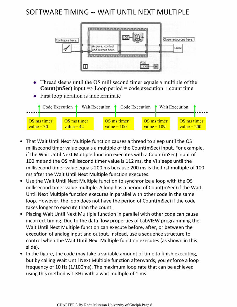
Thread sleeps until the OS millisecond timer equals a multiple of the Count(mSec) input => Loop period = code execution + count time

First loop iteration is indeterminate

OS ms timer value = 30





Code Execution Wait Execution Code Execution Wait Execution

That Wait Until Next Multiple function causes a thread to sleep until the OS millisecond timer value equals a multiple of the Count(mSec) input. For example, if the Wait Until Next Multiple function executes with a Count(mSec) input of 100 ms and the OS millisecond timer value is 112 ms, the VI sleeps until the millisecond timer value equals 200 ms because 200 ms is the first multiple of 100 ms after the Wait Until Next Multiple function executes.

•

Use the Wait Until Next Multiple function to synchronize a loop with the OS millisecond timer value multiple. A loop has a period of Count(mSec) if the Wait Until Next Multiple function executes in parallel with other code in the same loop. However, the loop does not have the period of Count(mSec) if the code takes longer to execute than the count.

•

Placing Wait Until Next Multiple function in parallel with other code can cause incorrect timing. Due to the data flow properties of LabVIEW programming the Wait Until Next Multiple function can execute before, after, or between the execution of analog input and output. Instead, use a sequence structure to control when the Wait Until Next Multiple function executes (as shown in this slide).

•

In the figure, the code may take a variable amount of time to finish executing, but by calling Wait Until Next Multiple function afterwards, you enforce a loop frequency of 10 Hz (1/100ms). The maximum loop rate that can be achieved using this method is 1 KHz with a wait multiple of 1 ms.

•



Add a Wait before the loop to initialize the timer Even first iteration of loop timer is deterministic with this

method

13

Wait Execution Code Execution Wait Execution Code Execution

100 112 200 209

Because Wait Until Next Multiple only accepts integers, loop rates are limited to only a few frequencies: 1000, 500, ~333, 250, 200, ~167 Hz, and so on.

•

In this figure, the 100 ms timer is initialized by calling the Wait Until Next Multiple function immediately before the While Loop begins. Otherwise, the loop time for the first iteration would be indeterminate. In the While Loop, the Wait Until Next Multiple function is enclosed in a sequence structure to assure that the delay is added after the code has finished. In this way, the order of execution is guaranteed.

•

Before deciding on a millisecond multiple, you must ensure that the code in your loop can execute faster than the wait multiple. If your code takes slightly longer than the ms multiple, then your loop actually waits 2 times ms multiples, because code was running when the first ms multiple arrived. In this case, the wait until ms multiple is not aware that the first ms multiple occurred and waits until a second ms multiple occurs before returning.

•

In addition to controlling loop rates, the Wait Until Next Multiple function forces time‐critical VIs to sleep until the wait is finished. When a VI sleeps, it relinquishes the CPU, allowing other VIs or threads to execute. Sleep time is required in time‐critical VIs, because the user interface and other background processes need CPU time to survive.

•



TWC (worst case execution time) < ΔT (millisecond multiple +jitter)

SW timing, ΔT = 5 ms +/- inherent jitter

Code execution time, Te

Worst case software jitter, Tj

Worst case time, Twc

The Wait Until Next Multiple function masks software jitter within the loop. The function has some inherent jitter, which is acceptable for many real‐time applications.

•

In this example, the Wait Until Next Multiple function synchronizes with each 5 ms tick of the OS clock, allowing the loop to achieve 200 Hz software‐timed analog input.

•

The timeline illustrates the 5 ms wait multiple at ΔT, the actual time required to execute the code at Te, worst case jitter at Tj, and worst case time at Twc. As long as the worst case time is smaller than the wait multiple, the actual loop period equals the wait multiple, plus or minus the jitter incurred by the function itself.

•


SOFTWARE TIMING ‐‐ TIMED LOOP

Use instead of a For or While Loop when appropriate

Choose the ms timer on the timed loop to use sw timing

Use the Timed loop to develop VIs with the following: Multi-rate timing capabilities; feedback on loop execution; timing

characteristics that change dynamically.

The Timed Loop applies only to Windows and ETS and executes an iteration of the loop at the period you specify. Use the Timed Loop when you want to develop VIs with multi‐rate timing capabilities, feedback on loop execution, or timing characteristics that change dynamically.

•

Because the Timed Loop automatically imposes sleep as needed to achieve the loop rate you specify, there is no need to use a Wait or Wait Until Next Multiple function to add sleep time in the loop.

•


HARDWARE TIMING ‐‐ NOT AVAILABLE ON [c]FieldPoint

Four standard methods of accomplishing hw timing Insert Wait function with µs resolution in loop

Insert Wait Until Next Multiple with µs resolution in loop

Replace loop with Timed Loop linked to µs clock or external clock

Use DAQmx VIs to connect to external clock

ConfigureAcquire

Control, andOutput

Close

Looping mechanism

The first 3 methods are similar to the software timing methods, but access a microsecond clock on the processor rather than the millisecond operating system clock.

•

The fourth method involves using DAQmx functions to connect to an external clock, such as the clock on a Multifunction DAQ device. You can use an external clock with the DAQmx VIs to time data acquisition or as an input on the Timed Loop.

•


HARDWARE TIMING ‐‐ us TIMING FUNCTIONS

Choose µs timing for the Wait function, Wait Until Next Multiple function, and Timed Loop to achieve greater loop rate resolution

Enables loop rates of 1 MHz, 500 KHz, ~333KHz, 250 KHz, 200 KHz, ~167 KHz, and so on.

Worst case code execution time must still be less than ΔT

Use same programming architecture as with software timing

If you are targeting to an RT target that allows microsecond timing, you can use the microsecond clock for the wait functions. If you are not targeted to an acceptable target, you can still select microsecond timing, but the program uses the millisecond OS clock instead.

•

With a ms clock, loop rates are 1/X ms = 1KHz, 500 Hz, ~333 Hz, 250 Hz, and so on

○

With a µs clock, loop rates are 1/X µs = 1 MHz, 500 KHz, ~333 KHz, 250 KHz, and so on

○

Using the microsecond clock allows for more loop rate options:

•


HARDWARE TIMING ‐‐ TIMED LOOP

Choosethe µ timer

Or connect an external clock

When you configure a Timed Loop, you can choose the MHz clock (us timer), if you are targeted to an appropriate target. You also can choose to connect an external clock to a terminal. You can access the configuration window by double‐clicking the Timed Loop.

•


HARDWARE TIMING ‐‐ DAQmx

Demo: NI Example FinderHardware Input and Output >> DAQmx >> Control >> General >> PID Control-Single Channel.vi

You can use NI data acquisition hardware and NI‐DAQmx to achieve a sleep resolution much finer than 1 kHz. Hardware timing uses the DAQ device internal clock or an external clock to control when a Read VI or a Write VI executes within a loop.

•

With a hardware timing, the loop rate matches the rate programmed into the Sample Clock VI. You must choose the Hardware Timed Signal Point sample mode input.

•

Overwrite errors can occur, however, when the requested scan rate is too fast relative to the code execution time. In other words, if the CPU is not powerful enough to execute the code within the loop at least as fast as the scan rate, the FIFO eventually overflows with new, unread data.

•


EVENT RESPONSE ‐‐MONITORING FOR EVENTS

Use the point-by-point VIs to monitor for the events such as: Triggering datalogging

Triggering an alarm

Performing a calculation

With real‐time event response, you can respond to a single event within a given amount of time. However, to respond to an event, the VI must know that the event has happened.

•

Some common events include detecting a peak in measurement or detecting when a threshold has been reached. You can use the Point‐by‐Point Signal Analysis VIs to watch for these types of events.

•


EVENT RESPONSE ‐‐ DIGITAL CHANGE DETECTION

Common event response application

Must have a digital I/O device that supports change detection

NI‐DAQmx only. Another common event response application involves watching for a digital line change, which is useful when watching for an alarm trigger. The slide above uses the DAQmx digital change functionality with the Timed Loop.

•

Notice that the digital line is connected to the clock terminal of the Timed Loop. When the digital change happens or a timeout occurs, the timed loop wakes up and processes the code in the loop.

•


COMMUNICATIONFront Panel Communication•Network Communication Methods•Communication Programming•LabVIEW Real‐Time Wizards•

The RT Engine on the RT target does not provide a user interface for applications.

•

You can use one of two communication protocols, front panel communication or network communication, to provide a user interface on the host computer for RT target VIs.

•


FRONT PANEL COMMUNICATION

With front panel communication, LabVIEW and the RT Engine execute different parts of the same VI, as shown in the slide above. LabVIEW on the host computer displays the front panel of the VI while the RT Engine executes the block diagram. A user interface thread handles the communication between LabVIEW and the RT Engine.

•

Use front panel communication between LabVIEW on the host computer and the RT Engine to control and test VIs running on an RT target. After downloading and running the VIs, keep LabVIEW on the host computer open to display and interact with the front panel of the VI.

•

You can also use front panel communication to debug VIs while they run on the RT target. You can use LabVIEW debugging tools – such as probes, execution highlighting, breakpoints, and single stepping – to locate errors on the block diagram code.Front panel communication is a good communication method for monitoring and interfacing with VIs running on an RT target. However, front panel communication is not deterministic and can affect the determinism of a time‐critical VI. Use network communication methods to increase the efficiency of the communication between a host computer and VIs running on the RT target.

•


NETWORK COMMUNICATION


To run another VI on the host computer○To control the data exchanged between the host computer and the RT target. You can customize the communication code to specify which front panel objects get updated and when. You also can control which components are visible on the front panel, because some control and indicators might be more important than others.

○

To control timing and sequencing of the data transfer.○To perform additional data processing or logging.○

NETWORK COMMUNICATION ‐‐ with network communication, a host VI runs on the host computer and communicates with the VI running on the RT target using specific network communication methods such as network‐published, shared variables, TCP, VI Server, and in the case of non‐networked RT Series plug‐in devices, shared memory reads and writes. You might use network communication for the following reasons:

In the diagram, the RT target VI is similar to the VI shown in the Front Panel Communication section, which runs on the RT target using front panel communication to update the front panel controls and indicators. However, the RT target VI in the figure above uses RT FIFO VIs to pass data to a communication VI. The communication VI then communicates with the host computer VI using network communication methods to update controls and indicators.

•


NETWORK COMMUNICATION METHODS

Protocol Programming Difficulty

Speed Architecture Caveats

TCP Good Better Client/Server

StringData

UDP Good Best Broadcast or Client/Server

Unreliable,String data

SharedVariable

Best Good Publisher/Subscriber

NI protocolLabView 8+

VI Server Better Poor Client/Server

LabVIEWonly

The network communication methods most commonly used with LabVIEW RT include TCP, UDP, shared variables, and VI server. Other methods, mostly used in legacy systems include DataSocket and Logos.

•

TCP – Protocol most commonly used for large systems. Provides a good mixture of speed and reliability. Data must be formatted as strings.

•

UDP – Fastest network protocol. Includes little error checking and can loose packets. Robust systems must implement their own error checking. Data must be formatted as strings.

•

Shared Variables – Easiest protocol to implement. Shared variables can be used deterministically directly from a time‐critical loop, because they implement a normal‐priority communication loop automatically. Only host programs using LabVIEW and other NI products can access shared variables that are only available on LabVIEW 8.0 and later.

•

VI Server – You can use VI server to run VIs and/or access and set the value of controls and indicators. VI Server communication is not recommended for transferring large amounts of data.

•

ArchitecturesClient – Server – a dedicated connection is created between a client and a server.•Broadcast – Application broadcasts data onto a network, any listeners can receive the data. Typically a one way conduit.Publisher/Subscriber – A server or program publishes data items. Subscribers subscribe to data items. Each subscriber can read and/or write to the data item.

•


chapter 3 by radu muresan university of guelph 3 lecture 4...chapter 3 by radu muresan university of...

Documents