33

CHAPTER 3

FUZZY LOGIC CONTROLLER BASED ACTIVE

SUSPENSION SYSTEM

3.1 INTRODUCTION

Vehicle suspension system is complex and highly nonlinear.

Suspension parameters (suspension deflection, sprung mass velocity, sprung

acceleration) will change when a vehicle rides on various road conditions.

Conventional control strategies depend on accurate system model and cannot

adapt to environmental conditions. Optimal controller discussed in the earlier

chapter is based on the linearized state space model. It suffers from the

limitation of accurate sensing and estimation of state variables for practical

implementation of suspension system. Hence a new controller is proposed to

overcome the above drawback of model dependency. Fuzzy Logic Controller

(FLC) design is discussed in this chapter as it is successful in kinds of

situation like (i) very complex models where understanding is strictly limited

or quite judgmental and (ii) processes where human reasoning, human

perception is inextricably involved.

FLC is used for disturbance rejection control to reduce unwanted

vehicle’s motion in active suspension system (Ting et al (1995)). Nonlinearity

is handled by rules, membership functions and the inference process which

results in improved performance. Literatures point that lot of work has been

done on FLC based active suspension system where the membership

functions are determined by trial and error method. Literatures have already

34

discussed about FLC and binary GA optimization (Kuo and Tzuu-Hseng

(1999)) and hence an alternate algorithm is sought for tuning the FLC

parameters which can overcome the drawback (converge to a local optima

rather than global optima) of GA. Real coded GA is used as it is very popular for

solving real valued optimization problems. Particle Swarm Optimization (PSO) is

a population based stochastic optimization technique and is becoming popular

due to its simplicity of implementation and ability to quickly converge to a

reasonably good solution (Chatterjee et al (2005)). Hence, it is proposed to

optimize the membership functions and scaling factors of FLC by PSO, real

coded GA and compare their performance in terms of ride comfort of the

vehicle suspension system.

3.2 FUZZY LOGIC CONTROL

FLC is based on the general principles of fuzzy set theory and

introduced by Zadeh (1965). Fuzzy set theory provides a means for

representing uncertainties. Fuzzy concept has been widely used in control

system design.

3.2.1 Structure of Fuzzy Logic Controller

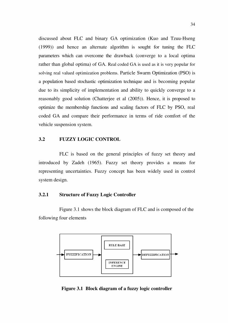
Figure 3.1 shows the block diagram of FLC and is composed of the

following four elements

Figure 3.1 Block diagram of a fuzzy logic controller

35

1. A fuzzification interface, which converts controller inputs into

information that the inference mechanism can easily use to

activate and apply rules.

2. A rule-base (a set of If-Then rules), which contains a fuzzy

logic quantification of the expert’s linguistic description of

how to achieve good control.

3. An inference mechanism (also called an “inference engine” or

“fuzzy inference” module), which emulates the expert’s

decision making in interpreting and applying knowledge about

how best to control the plant.

4. A defuzzification interface, which converts the conclusions of

the inference mechanism into actual inputs for the process.

The number of necessary fuzzy sets and their ranges are designed

based upon the experience gained on the process.

3.2.2 GA/PSO Optimized Fuzzy Logic Controller

The controller structure adopted in this study is shown in

Figure 3.2. Suspension deflection and sprung mass velocity are provided as

the inputs to the fuzzy controller and actuator force is taken as the controller

output. GE, GV and GU are the scaling factors of the FLC. Position of the

Vertex (VP) of the triangular membership function to be optimized by

GA/PSO techniques are shown in Figure 3.3. Vp1 to Vp5 refers to the

suspension deflection membership function, Vp6 to Vp10 represents sprung

mass velocity membership function and Vp11 to Vp15 corresponds to output

force membership function. RMS value of the body acceleration is taken as

the performance index as it reflects the ride comfort of the suspension system.

GA/PSO algorithm tunes the scaling factors and the membership functions of

the input and output variables.

36

Figure 3.2 Block diagram of the GA/PSO FLC structure

Figure 3.3 Vertex points in membership functions

3.2.3 Fuzzy Inputs and Output variables

The universe of discourse for the input variables are found by

subjecting the passive suspension to different input conditions and viewing

the maximum and minimum values for each particular input variable. The

universe of discourse for the output variable is chosen by using engineering

judgment and reasonable maximum force for an actuator.

37

The universe of discourse for both the input and output variables are

classified into five fuzzy sets namely Negative Large (NL), Negative Small

(NS), Zero (Z), Positive Small (PS) and Positive Large (PL). Triangular

membership functions are used in the control design as there exist an

appreciable change in the output for slight variations in the input variable and

are shown in Figure 3.4. Both the input and output variables are defined on

the normalized domain of [-1 1].

GE, GV and GU are the scaling factors of suspension deflection,

sprung mass velocity and actuator force respectively. Fuzzy rule base is in the

form of the linguistic variables using the fuzzy conditional statement. It is

composed of the antecedent (If-clause) and the consequence (Then - clause).

For example, “IF suspension deflection is NS and the sprung mass velocity is

PS, THEN the actuator force is ZE ". Each rule is derived from the

characteristic of the active suspension system. Fuzzy rule base is a

combination of all possible control rules and it is summarized in Table 3.1.

Mamdani's minimum operation is used as a fuzzy implication function. Centre

of gravity method is used to defuzzify the inferred output.

Figure 3.4 Membership functions - input/output variables

38

Table 3.1 FLC Rule base

Suspension

Deflection

Sprung MassVelocity

NL NS Z PS PL

NL PL PL PS PS Z

NS PL PS PS Z NS

Z PS PS Z NS NS

Ps PS Z NS NS NL

PL Z NS NS NL NL

3.3 OPTIMIZATION TECHNIQUES

The design of a FLC is not straightforward, because of the

heuristics involved in control rules and membership functions. Currently,

there are no systematic methods for the design of the fuzzy knowledge base or

for the tuning of the fuzzy controller’s parameters. Therefore, the designers

have to devise a fuzzy knowledge base using heuristic methods and

experience. The parameters of a fuzzy control system are tuned by means of a

trial and error method. In this work, scaling factors and membership functions

of the FLC are tuned using GA and PSO techniques. Tunable parameters are

the three scaling factors GE, GV, GU and Vp of the triangular membership

functions.

3.3.1 GA tuning of FLC

Genetic algorithms are adaptive search techniques based on the

“survival of the fittest” biological concept. They can yield an efficient and

effective way for optimization applications by searching for a global

minimum without the need of derivative of a cost function (Lin and Huang

39

(2003)). GA consists of three main operations namely Selection, Crossover

and Mutation and create a new individual which may be better than their

parents. This algorithm repeats for many generations and finally stops while

reaching individuals that represent the optimum solution to the problem. The

flowchart of GA is shown in Figure 3.5.

Figure 3.5 GA flow chart

Due to its effectiveness in searching nonlinear, multi-dimensional

search spaces, GA is applied to the tuning of the scale factors and

40

membership functions of the FLC to ensure optimal control performance at

nominal operating conditions. Since the tuned parameters are real numbers,

real coded GA is applied for evolution. Real coded numbers are combined

together as a string or structure and are called as a chromosome while each

number of the chromosome is a gene. GA starts with a population of n

randomly generated structures, where each structure encodes a solution of the

problem. The cost function used to evaluate the individuals of each generation

is chosen as the RMS of sprung mass acceleration. During the search process

GA looks for the optimal solution which minimizes the cost function. The

overall fitness which the GA aims to maximize is computed as

F= 1000 / (1+J) (3.1)

where J is the cost function. The effectiveness of the technique is shown by

simulation. The GA parameters are given in Table 3.2.

Table 3.2 Parameters of GA algorithm

No. of generations 70

Population size 12

Type of crossover Single point

cross over

mutation rate 0.15

Upper and lower bounds of GE,GV and

GU

[0 5]

Upper and lower bounds of VP1 – VP15 [-1 1]

3.3.2 PSO tuning of FLC

Particle Swarm Optimization (PSO) is a population based

stochastic optimization technique developed by Kennedy and Eberhart (1995)

inspired by the social behaviour of bird flocking or fish schooling. PSO shares

41

many similarities with evolutionary computation techniques. However, unlike

GA, PSO has no evolution operators such as crossover and mutation. In PSO,

the potential solutions, called particles, fly through the problem space by

following the current optimum particles.

The PSO algorithm is becoming popular due to its simplicity of

implementation and ability to quickly converge to a reasonably good solution

(Eberhart and Shi (2001)). PSO has been successfully applied in many areas

like function optimization, artificial neural network and fuzzy logic control

etc. In this algorithm, the individual is called particle and the trajectory of

each individual in the search space is adjusted dynamically by altering the

velocity of each particle, according to its own flying experience and the flying

experience of the other particles in the search space.

Modification of the searching point of a PSO algorithm is shown in

Figure 3.6. Let x and v denote a particle coordinates (position) and its

corresponding flight speed (velocity) in a search space, respectively.

k

iv

1k

iv

1k

ix

pbest

iv

gbesti

pbestik

ix

gbest

iv

Figure 3.6 Modification of a searching point by PSO

x : current position, x : modified position

v : current velocity, v : modified velocity,

v : velocity based on pbest,

v : velocity based on gbest.

42

PSO is initialized with a group of random particles (solutions) and

then searches for optima by updating generations. In every iteration, each

particle is updated by following two "best" values. The first one is the best

solution (fitness) it has achieved so far and is represented as pbest. Another

“best” value is the best solution obtained by any particle in the population.

This is represented as gbest. Each particle knows the best value so far (pbest)

and best value in the group (gbest). The particle tries to modify its position

using the current velocity and the distance from pbest and gbest. The

modified velocity and position of each particle is evaluated using the

following expression (Gaing (2004))

v = w v + c rand (pbest x ) + c rand (gbest x ) (3.2)

x = x + v (3.3)

w - inertia weight parameter

c1, c

2 - weight factors

rand1, rand

2- random number between 0 and 1

v - velocity of particle i in kth

iteration

x - position of particle i in kth

iteration

Suitable selection of w provides a balance between global and local

explorations and it is set according to the following equation

w = wmax

– ((wmax

- wmin

)* t / T) (3.4)

where w is an adjustable parameter between wmax

and wmin

wmax - maximum inertia weight

43

wmin - minimum inertia weight

t - current iteration number

T - maximum number of iterations

Start

Calculate parameters of Fuzzy logic

controller GE,GV and GU

Calculate the fitness

function

Update Velocity, Position

Gbest and Pbest of particles

Calculate Pbest of each particle and

gbest of population

Maximum iteration

number reached ?

Stop

No

Yes

Generate initial populations

Figure 3.7 Flow chart of PSO algorithm

The flowchart of PSO algorithm is shown in Figure 3.7. Generating

initial populations is the first step of PSO. The population is composed of the

particles that are real codes. The corresponding evaluation of a population is

the “fitness function”. The RMS value of sprung mass acceleration is taken

as the performance index and the fitness function is given by Equation (3.1).

44

After the fitness function has been calculated, the fitness value and

the number of the iterations determine the stopping condition. The pbest of

each particle and gbest of population (the best movement of all particles) are

calculated. Updating the velocity, position, gbest and pbest of particles give a

new best position.

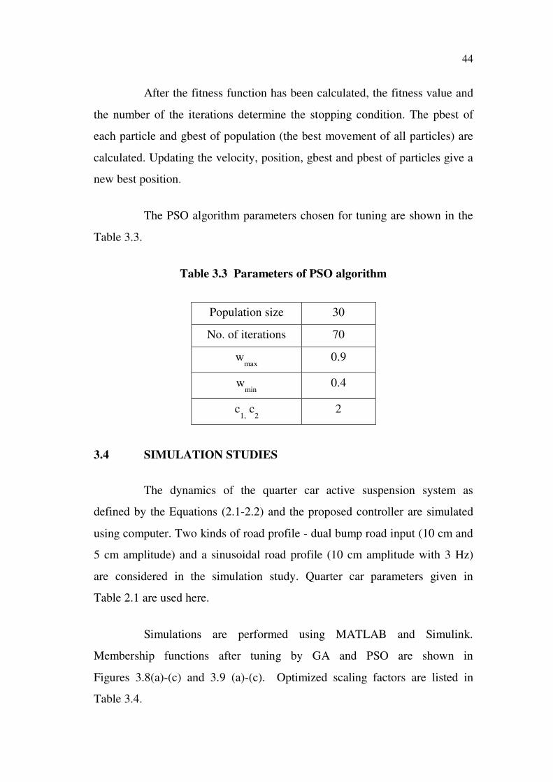
The PSO algorithm parameters chosen for tuning are shown in the

Table 3.3.

Table 3.3 Parameters of PSO algorithm

Population size 30

No. of iterations 70

wmax

0.9

wmin

0.4

c1,

c2

2

3.4 SIMULATION STUDIES

The dynamics of the quarter car active suspension system as

defined by the Equations (2.1-2.2) and the proposed controller are simulated

using computer. Two kinds of road profile - dual bump road input (10 cm and

5 cm amplitude) and a sinusoidal road profile (10 cm amplitude with 3 Hz)

are considered in the simulation study. Quarter car parameters given in

Table 2.1 are used here.

Simulations are performed using MATLAB and Simulink.

Membership functions after tuning by GA and PSO are shown in

Figures 3.8(a)-(c) and 3.9 (a)-(c). Optimized scaling factors are listed in

Table 3.4.

45

Table 3.4 Optimized scaling factors

Optimization

algorithmGE GV GU

GA 1.0387 4.9373 3.9011

PSO 0.1001 4.9813 1.4962

Figure 3.8 (a) GA tuned suspension deflection

Figure 3.8 (b) GA tuned sprung mass velocity

Figure 3.8 (c) GA tuned force

46

Figure 3.9 (a) PSO tuned Suspension deflection

Figure 3.9 (b) PSO tuned Sprung mass velocity

Figure 3.9 (c) PSO tuned force

47

Simulations are conducted for open loop passive, active

suspension with FLC, GA tuned FLC and PSO tuned FLC. All the relevant

parameters and conditions are maintained the same for all the schemes to

ensure a realistic and a fair one-to-one comparison.

Figures 3.10-3.13 illustrates the simulation results for the passive,

FLC, GAFLC and PSOFLC based active suspension system for the bump

road input. Figure 3.10 indicates the reduction in sprung mass displacement

by both PSOFLC and GAFLC. The minimum sprung mass displacement is

exhibited by real coded GA tuned FLC. Figure 3.11 shows that the body

acceleration is reduced by 100% by the GAFLC compared to its counterparts.

Figure 3.12 indicates that the suspension deflection controlled by GAFLC and

PSOFLC exceed the limit of ± 8cm. Figure 3.13 illustrates the road holding

ability maintained by the PSOFLC scheme is superior to that of others. Tyre

deflection exhibited by GAFLC is worst than passive.

Figure 3.10 Sprung mass displacement – bump input

48

Figure 3.11 Sprung mass acceleration – bump input

Figure 3.12 Suspension deflection– bump input

Figure 3.13 Tyre deflection – bump input

49

Figures 3.14-3.17 present the simulation results for the sinusoidal

road input. Figure 3.14 demonstrate that the sprung mass position of the

vehicle body by PSOFLC scheme oscillates around 1cm and its displacement

is completely brought down by the GAFLC. Figure 3.15 shows that the body

acceleration is reduced by 95.8% compared to passive and 86.84% compared

to PSOFLC by the GAFLC. Thus the GAFLC scheme guarantees better ride

comfort. Figure 3.16 indicates that the suspension deflection controlled by

GAFLC and PSOFLC is of same magnitude but smaller than that of passive.

Figure 3.17 illustrates a smaller tyre deflection for PSOFLC and thus the road

holding ability is maintained by the same. The performance of the active

suspension system clearly indicates the superiority of the GAFLC scheme

over its counterparts.

Figure 3.14 Sprung mass displacement – sinusoidal input

50

Figure 3.15 Sprung mass acceleration – sinusoidal input

Figure 3.16 Suspension deflection– sinusoidal input

Figure 3.17 Tyre deflection – sinusoidal input

51

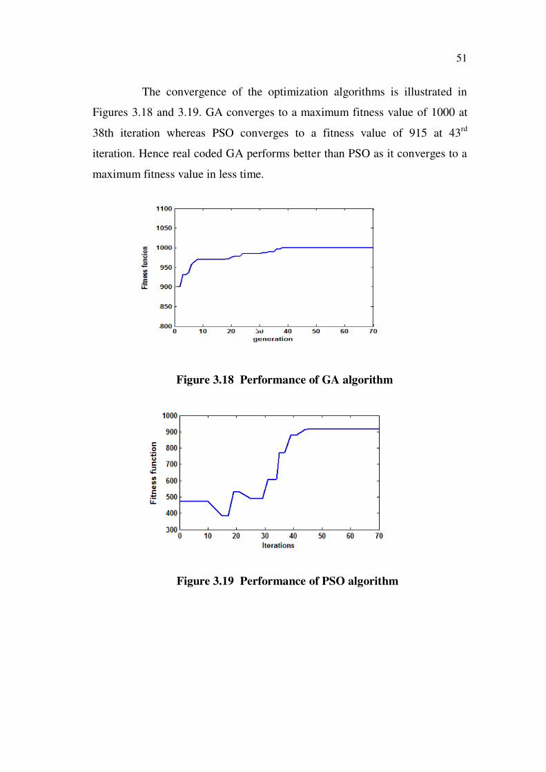
The convergence of the optimization algorithms is illustrated in

Figures 3.18 and 3.19. GA converges to a maximum fitness value of 1000 at

38th iteration whereas PSO converges to a fitness value of 915 at 43rd

iteration. Hence real coded GA performs better than PSO as it converges to a

maximum fitness value in less time.

Figure 3.18 Performance of GA algorithm

Figure 3.19 Performance of PSO algorithm

52

3.4.1 Comparison of GAFLC with PSOFLC

The comparison of the controllers is presented in Table 3.5, which

shows the RMS value of the body acceleration, suspension deflection, body

displacement and tyre deflection. The results show that proposed GAFLC

scheme outperforms the conventional passive, FLC and PSOFLC in providing

desired ride comfort. However road handling is best exhibited by PSOFLC.

Table 3.5 RMS values of the time responses of the Quarter car model

Input Controller

Sprung Mass

Displacement

10-3

(m)

Suspension

Deflection

10-2

(m)

Body

Acceleration

(m/s2)

Tyre

deflection

10-3

(m)

Bump

Input

Passive 19.56 1.776 1.571 2.667

FLC 8.693 1.32 0.9229 2.32

GAFLC2.836 1.505 0 2.776

PSOFLC4.3 1.476 0.2179 2.357

Sinusoidal

Road profile

Passive 25.57 8.307 8.46 11.61

FLC13.57 7.541 4.767 11.32

GAFLC0.7259 7.599 0.3499 11.42

PSOFLC6.798 7.663 2.666 8.149

3.4.2 Power Spectral Density of Sprung Mass Acceleration

Power Spectral Density (PSD) describes how the power of a signal

or time series is distributed with frequency. The power here can be the actual

physical power, or more often can be defined as the squared value of the

53

signal. This instantaneous power (the mean or expected value of which is the

average power) is then given by

P(t) = s(t) (3.5)

for a signal s(t). In the evaluation of vehicle ride quality, the PSD of the

sprung mass acceleration as a function of frequency is of prime interest and is

shown in Figures 3.20 and 3.21 for both inputs.

Figure 3.20 PSD of sprung mass acceleration – bump input

Figure 3.21 PSD of sprung mass acceleration – sinusoidal input

54

Both GA and PSO tuned FLC have significantly suppressed the

acceleration of sprung mass effectively in the low frequency band. It can be

observed from the PSD plot that the sprung mass acceleration has been

brought down within the frequency range of 0.4 Hz to 8 Hz for sinusoidal

input and the entire low frequency region for bump input by the GAFLC

scheme. Both optimization techniques perform much better than passive and

FLC. GAFLC exhibits superior performance especially in the human sensitive

frequency range of 4 Hz to 8 Hz.

Table 3.6 Comparison of ride characteristics

Seok-il and Isik

(1996)

Bump input

(20km/hr)FLC

65 % reduction in Body acceleration.

43% reduction in Tyre Deflection.

Dae and Nizar

(1995)

Sinusoidal with

random noiseFLC

47% reduction in Body acceleration

35% reduction in Tyre Deflection.

Author

Bump input

(20km/hr)

PSOFLC86% reduction in Body acceleration

13.7% reduction in Tyre Deflection

GAFLC100% reduction in Body acceleration

Poor Tyre deflection

FLC41% reduction in Body acceleration

13% reduction in Tyre Deflection

Sinusoidal, 3Hz.

PSOFLC68.5% reduction in Body acceleration

30% reduction in Tyre deflection

GAFLC 95.8 % reduction in Body acceleration

Poor Tyre deflection

FLC 44% reduction in Body acceleration

3% reduction in Tyre deflection

Table 3.6 gives the comparison of ride characteristics for the

proposed PSOFLC with the previous results available for FLC of active

suspension system. In the entire cases quarter car model is used. For similar

55

simulation parameters, ride comfort is enhanced by GAFLC whereas road

handling is improved by the FLC by Seok-il and Isik (1996). For sinusoidal

road profile, ride comfort improved by GAFLC and PSOFLC scheme is

around 48.8% and 12% respectively more than the method by Dae and Nizar

(1995). But the tyre deflection is more pronounced in the case of GAFLC

compared to FLC. This table proves the effectiveness of the GAFLC in

improving the ride comfort of the vehicle suspension system.

3.5 CONCLUSION

This chapter discussed the design of FLC for active suspension

system. Performance of FLC is optimized with GA and PSO algorithms for

enhancement in ride comfort and their performances are compared. From the

simulation results it is obvious that there is an enhancement in the ride-

comfort by the GAFLC based active suspension system. Compared with PSO,

real coded GA algorithm also has significant performance of convergence.

Contrast to full state LQR, proposed FLC applies only two states for control

and attains a better performance.