chapter 3 individual income taxation income... · 2018-03-29 · chapter 3 . individual income...

Lectures on Public Finance Part2_Chap3, 2018 version P.1 of 43 Last updated 28/03/2018

Chapter 3 Individual Income Taxation

3.1 Introduction The individual income tax is the most important single tax in many countries. The basic principle of the individual income tax is that the taxpayer’s income from all sources should be combined into a single or global measure of income. Total income is then reduced by certain exemptions and deductions to arrive at income subject to tax (i.e. taxable income). This is the base to which tax rate are applied when computing tax.

A degree and coverage of exemptions and deductions vary from country to country. A degree of progressivity of tax rates also varies.

Nevertheless the underlying principles of the tax system are common among countries and are worth reviewing.

3.2 The Income-Based Principle Economists have argued that a comprehensive definition of income must be used that includes not only cash income but capital gains. A number of other adjustments have to be made to convert your “cash” income into the “comprehensive” income that, in principle, should form the basis of taxation.

This comprehensive definition of income is referred to as the Hicksian concept or the Haig-Simons concept. This concept measures most accurately reflects “ability to pay”.

(1) Cash basis: In practice, only cash-basis market transactions are taxed. The tax is thus levied on a notion of income that is somewhat narrower than that which most economists would argue. Certain non-marketed (non-cash) economic activities are excluded, though identical activities in the market are subject to taxation (e.g. housewife’s work at home (vis-à-vis a maid’s work), and own house (vis-à-vis rented house)).

Some non-cash transactions are listed in the tax code but are difficult to enforce. Barter arrangements are subject to tax.

Unrealized capital gains is also not included in the income tax bases. Capital gains are taxed only when the asset is sold (not on an accrual basis).

(2) Equity-based adjustments: Individuals who have large medical expenses or casualty losses are allowed to deduct a portion of those expenses from their income, presumably


on the grounds that they are not in as good a position for paying taxes as someone with the same income without those expenses.

(3) Incentive-based adjustments: The tax code is used to encourage certain activities by allowing tax credits or deductions for those expenditures. Incentives are provided for energy conservation, for investment, and for charitable contributions.

(4) Special Treatment of Capital Income: The tax laws treat capital and wage income separately. The difficulty of assessing the magnitude of the returns to capital plays some role, while attempts to encourage savings as a source of domestic investment and growth.

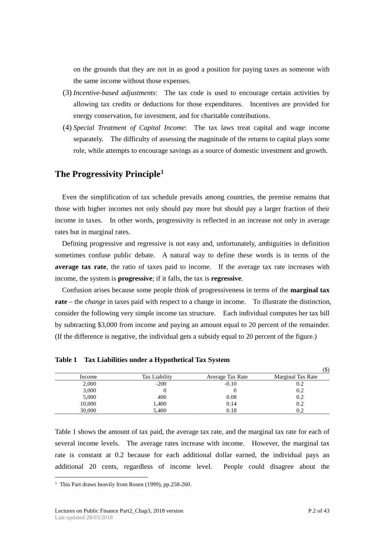
The Progressivity Principle1 Even the simplification of tax schedule prevails among countries, the premise remains that those with higher incomes not only should pay more but should pay a larger fraction of their income in taxes. In other words, progressivity is reflected in an increase not only in average rates but in marginal rates. Defining progressive and regressive is not easy and, unfortunately, ambiguities in definition sometimes confuse public debate. A natural way to define these words is in terms of the average tax rate, the ratio of taxes paid to income. If the average tax rate increases with income, the system is progressive; if it falls, the tax is regressive. Confusion arises because some people think of progressiveness in terms of the marginal tax rate – the change in taxes paid with respect to a change in income. To illustrate the distinction, consider the following very simple income tax structure. Each individual computes her tax bill by subtracting $3,000 from income and paying an amount equal to 20 percent of the remainder. (If the difference is negative, the individual gets a subsidy equal to 20 percent of the figure.) Table 1 Tax Liabilities under a Hypothetical Tax System

($) Income Tax Liability Average Tax Rate Marginal Tax Rate

2,000 -200 -0.10 0.2 3,000 0 0 0.2 5,000 400 0.08 0.2

10,000 1,400 0.14 0.2 30,000 5,400 0.18 0.2

Table 1 shows the amount of tax paid, the average tax rate, and the marginal tax rate for each of several income levels. The average rates increase with income. However, the marginal tax rate is constant at 0.2 because for each additional dollar earned, the individual pays an additional 20 cents, regardless of income level. People could disagree about the 1 This Part draws heavily from Rosen (1999), pp.258-260.


progressiveness of this tax system and each be right according to their own definitions. It is therefore very important to make the definition clear when using the terms regressive and progressive. In the remainder of this section, we assume they are defined in terms of average tax rates. The degree of progression Progression in the income tax schedule introduces disproportionality into the distribution of the tax burden and exerts a redistributive effect on the distribution of income. In order to explore these properties further, we need to be able to measure the degree of income tax progression along the income scale. Such measures are called measures of structural progression (sometimes, measures of local progression). There is more than one possibility, as we will see. Each such measure will induce a partial ordering on the set of all possible income tax schedules. We could not expect always to be able to rank a schedule )(2 xt unambiguously more, or less, structurally progressive than another schedule )(1 xt : we must

allow that a schedule could display more progression in one income range and less in another. Nevertheless, the policymaker and tax practitioner, and indeed the man in the street, would like to be able to say which of any two alternative income tax systems is the more progressive in its effects. Is the federal income tax in the USA more redistributive than the personal income tax in Germany? This sort of question will take us from measures of structural progression to measures of effective progression. Measuring effective progression is a matter of reducing a tax schedule and income distribution pair to a scalar index number. The same schedule )(xt

could be more progressive in effect when applied to distribution A than to distribution B. Trends in effective progression for a given country over time, as well as differences between the income taxes of different countries, can be examined using such index numbers. Let us begin by defining as )(xm and )(xa respectively the marginal and average rates of

tax experienced by an income x :

xxtxa )()( = and )(')( xtxm = (1)

Since

xxaxm

xxtxxt

xxxtd )()()()('

d/)]([

2−

=−

= (2)

for strict progression it is necessary and sufficient that


xxaxm allfor )()( > (3)

The strict inequality rules out the possibility that the tax could be proportional to income in any interval: we may relax it if we wish. Measures of structural progression quantify, in various ways, the excess of the marginal rate )(xm over the average rate )(xa at income level x .

We introduce two particularly important measures here. First, liability progression )(xLP is defined at any income level x for which 0)( >xt as

the elasticity of tax liability to pre-tax income:

1)()(

)()(')( ),( >===

xaxm

xtxxtexLP xxt (4)

As we have already noted, for a strictly progressive income tax a 1 percent increase in pre-tax income x leads to an increase of more than 1 percent in tax liability. )(xLP measures the actual percentage increase experienced. A change of tax schedule which, for some 0x , casues an increase in )( 0xLP connotes, in an obvious sense, an increase in progression at that income level 0x . If the change in a strictly positive income tax involves an upward shift of the entire

function )(xLP , then the tax has become everywhere more liability progressive. Second, residual progression )(xRP is defined at all income levels x as the elasticity of

post-tax income to pre-tax income:

1)(1)(1

)()]('1[)( ),( <

−−

=−−

== −

xaxm

xtxxtxexRP xxtx (5)

The counterpart to the observation above is that a 1 percent increase in pretax income x leads t oan increase of less than 1 percent in post-tax income. )(xRP measures the actual percentage increase in post-tax income. A reduction in )(xRP must clearly be interpreted as an increase

in progression, according to this measure. These measures were first proposed by Musgrave and Thin (1948). It is inconvenient that

)(xRP should decrease when the tax becomes more progressive. We therefore make a minor

change of definition in this book, which is not standard in all of the literature, replacing the measure )(xRP by its reciprocal:

1)(1)(1

)(1)(* >

−−

==xmxa

xRPxRP (5a)


)(* xRP can be interpreted as the elasticity of pre-tax income to post-tax income. An increase in )(* xRP makes the tax more residually progressive at x .

Each of these measures quantifies in its own way the excess of the marginal rate of tax over the average rate of tax at the income level x , and accordingly induces a different partial ordering on the set of all tax schedules. Equipped with these measures, we shall, in the next two sections of the chapter, be able to demonstrate that if the income tax becomes structurally more progressive, and the pre-tax income distribution does not change, then this implies enhanced deviation from proportionality (in the case of liability progression) and enhanced redistributive effect (in the case of residual progression).

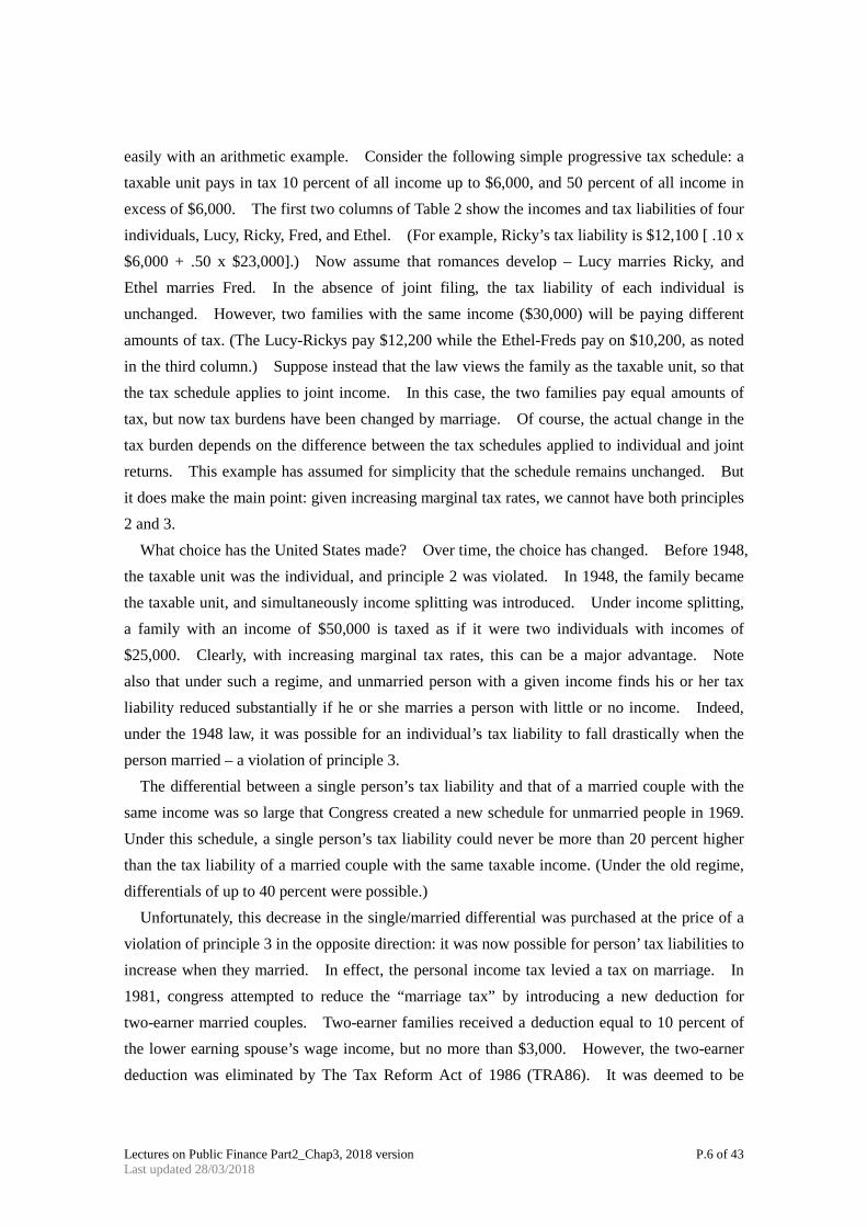
3.3 The Individual or Family-Based Principle: Choice of Unit2 The basic unit of taxation can be either the individual or the family. Many countries adopt the individual-based principle while some adopt the family-based principle. Background To begin, it is useful to consider the following three principles:

1. The income tax should embody increasing marginal tax rates. 2. Families with equal incomes should, other things being the same, pay equal taxes. 3. Two individuals’ tax burdens should not change when they marry; the tax system should

be marriage neutral. Table 2 Tax liabilities under a hypothetical tax system

($)

Individual Income Individual Tax Family Tax with Individual Filing Joint Income Joint Tax

Lucy 1,000 100 12,200 30,000 12,600 Ricky 29,000 12,100 Ethel 15,000 5,100 10,200 30,000 12,600 Fred 15,000 5,100

Although a certain amount of controversy surrounds the second and third principles, it is probably fair to say they reflect a broad consensus as to desirable features of a tax system. While agreement on the first principle is weaker, increasing marginal tax rates seem to have wide political support. Despite the appeal of these principles, a problem arises when it comes to implementing them: In general, no tax system can adhere to all three simultaneously. This point is made most 2 This Part draws heavily on Rosen (1999, Chap.16, pp.363-5).


easily with an arithmetic example. Consider the following simple progressive tax schedule: a taxable unit pays in tax 10 percent of all income up to $6,000, and 50 percent of all income in excess of $6,000. The first two columns of Table 2 show the incomes and tax liabilities of four individuals, Lucy, Ricky, Fred, and Ethel. (For example, Ricky’s tax liability is $12,100 [ .10 x $6,000 + .50 x $23,000].) Now assume that romances develop – Lucy marries Ricky, and Ethel marries Fred. In the absence of joint filing, the tax liability of each individual is unchanged. However, two families with the same income ($30,000) will be paying different amounts of tax. (The Lucy-Rickys pay $12,200 while the Ethel-Freds pay on $10,200, as noted in the third column.) Suppose instead that the law views the family as the taxable unit, so that the tax schedule applies to joint income. In this case, the two families pay equal amounts of tax, but now tax burdens have been changed by marriage. Of course, the actual change in the tax burden depends on the difference between the tax schedules applied to individual and joint returns. This example has assumed for simplicity that the schedule remains unchanged. But it does make the main point: given increasing marginal tax rates, we cannot have both principles 2 and 3. What choice has the United States made? Over time, the choice has changed. Before 1948, the taxable unit was the individual, and principle 2 was violated. In 1948, the family became the taxable unit, and simultaneously income splitting was introduced. Under income splitting, a family with an income of $50,000 is taxed as if it were two individuals with incomes of $25,000. Clearly, with increasing marginal tax rates, this can be a major advantage. Note also that under such a regime, and unmarried person with a given income finds his or her tax liability reduced substantially if he or she marries a person with little or no income. Indeed, under the 1948 law, it was possible for an individual’s tax liability to fall drastically when the person married – a violation of principle 3. The differential between a single person’s tax liability and that of a married couple with the same income was so large that Congress created a new schedule for unmarried people in 1969. Under this schedule, a single person’s tax liability could never be more than 20 percent higher than the tax liability of a married couple with the same taxable income. (Under the old regime, differentials of up to 40 percent were possible.) Unfortunately, this decrease in the single/married differential was purchased at the price of a violation of principle 3 in the opposite direction: it was now possible for person’ tax liabilities to increase when they married. In effect, the personal income tax levied a tax on marriage. In 1981, congress attempted to reduce the “marriage tax” by introducing a new deduction for two-earner married couples. Two-earner families received a deduction equal to 10 percent of the lower earning spouse’s wage income, but no more than $3,000. However, the two-earner deduction was eliminated by The Tax Reform Act of 1986 (TRA86). It was deemed to be


unnecessary because lower marginal tax rates reduced the importance of the “marriage tax.” Nevertheless, a substantial penalty still exists, and it tends to be highest when both spouses have similar earnings. Under certain conditions, for example, when two individuals with $25,000 adjusted gross income (AGIs) marry, their joint tax liability can increase by more than $700. On the other hand, when there are considerable differences in individuals’ earnings, the tax code provides a bonus for marriage. If two people with $10,000 and $50,000 AGIs marry, their joint tax liability can decrease by $1,100. In cases like these, the law provides a “tax dowry.”

3.4 The Annual Measure of Income Principle Income tax is usually based on annual income, not lifetime income. Economic theory is usually based on the lifetime utility maximization (e.g. life-cycle hypothesis), with the current annual income taxation, consumption smoothing does not avoid tax distortion. Because of the progressive nature of our tax system, the individual with the fluctuating income has to pay more taxes over his lifetime than the individual with a steady income.

The Basic Framework 1) The Criteria for Optimality Musgrave in his classic text book (The Theory of Public Finance (1959), McGraw-Hill) provides three criteria for appropriate taxation;

(a) the need for taxes to be fair; (b) the need to minimize administrative costs; and (c) the need to minimize disincentive effects.

The approach of the optimal taxation literature is to use economic analysis to combine the criteria into one, implicitly deriving the relative weights that should be applied to each criterion. This is done by using the concepts of individual utility and social welfare.

Economists found it very difficult to model the relationship between tax rates and administrative costs. They usually ignored administrative costs in their analysis and concentrated on criteria (a) and (c)3. Effectively, they tried to determine the tax system that will provide the best compromise between equality (fairness) and efficiency (incentives).

2) The Specification of Social Welfare

3 It is possible to include administrative costs in the tax analysis both in theory and in empirical investigations. It is

rather important to take administration into account in tax analysis.


As we discussed before, social welfare function can take many forms as policy makers have different policy objectives and welfare criteria.

If our idea of a fair tax system is one that reduces inequality of utility, our social welfare function must place more weight on utility gains of poor people than those of rich people.

This is achieved by using the following formulae,

( )( )

w u

u

h

h

h

h

=−

≠

= =

∑

∑

−11

1

εε

ε

ε for 1

for 1log (6)

where ε is a degree of inequality aversion. 3) The Modeling of Disincentives

In case of optimal income taxation in a model where labor supply response is the only disincentive problem, the utility function for each individual is used both to predict how that person will alter his/her labor supply when taxes are changed and to evaluate the resulting level of individual utility. The changes in labor supply will then be used to calculate the change in tax revenue, while the changes in utility will be used to calculate the change in social welfare. The optimal tax system will be the one where it is impossible to increase social welfare without reducing overall tax revenue.

The requirement to raise a specific amount of tax revenue is obviously fundamental. It has two important implications. First, it means that the solution to the optimal tax problem depends on the size of the revenue requirement. Second, it means that the tax changes that are considered should be revenue-neutral.

Why does it matter that a higher tax rate with higher personal allowances will reduce labor supply? After all, the objective is to maximize social welfare, not the size of the national income. The answer is that, by choosing to work less on average, workers will have lower incomes and thus will pay less taxes. Thus a change that would have been revenue-neutral for a fixed level of labor supply will, as a result of the reduction in work, produce a revenue loss. It is this revenue loss that represents the ‘excess burden’ of taxation. It requires an increase in tax rates to offset it – an increase that will reduce social welfare and counteract, at least in part, the gain is social welfare from the reduction in inequality that is produced by the increase is tax progressivity.

4) Problems of Application

The usefulness of the optimal tax results depends on the realism of the economic models. This is not to say that the presence of any unrealistic assumption invalidates the results. Rather,


any practical application of theoretical analysis requires an evaluation of whether any violation of the assumption can be expected to alter the results significantly.

Examples of unrealistic assumptions: (a) neglect of administrative and compliance costs of tax collection. (b) Assumption of perfect competition (c) neglect of heterogeneity of households in terms of their composition and preferences

What, then, the modern theory of income taxation ought to be concerned? 1. It must capture the efficiency/equity trade off involved in income taxation. 2. The structure of the income tax must be compatible with the revelation of the ability of

households. In a simpler term, the fundamental policy issue is whether it would be a good idea to

increase the rate of income tax and use the proceeds to fund an increase in tax allowances, thus reducing after-tax income inequality.

3.5 Optimal Income taxation4 A linear income tax schedule is one possibility for choosing an income tax. More generally, however, the structure of personal income taxation need not be linear with a constant rate of taxation, but rather marginal tax rates can vary with different levels of income. This is the case in practice. Suppose that we set out to determine the general optimal income tax structure that maximizes a social welfare function. We are then looking for a relationship between the tax rate and earned income that could in principle be progressive or regressive. If the rate of taxation, t, were to change with every change in income, we would be looking for an optimal income schedule )(Yft = (7)

If a linear income tax schedule were to maximize social welfare, this would be revealed as the solution to the general problem of optimal personal income taxation. We can expect the quest to identify a general structure of optimal income taxation as expressed by (7) to be complicated. In the case of the linear income tax, we had to find values for income subsidy S and t related through the government budget. In the case of the tax schedule (7), we are looking for a relationship between the tax rate and income that maximizes social welfare. That is, the solution to the general optimal taxation problem is a function that

4 This part quotes Hillman (2003, Chap.7, pp.479-83.)


tells us how to set the tax rate t for all values of income Y. We have seen that there are cases for both progressive and regressive taxes, and we therefore do not know beforehand whether the relationship expressed in (7) will indicate progressive or regressive taxation. We do know that finding an optimal income tax schedule requires a compromise between the progressive taxation sought for reasons of social justice (through the equal-sacrifice principle) and the efficiency and tax-base benefits of regressive taxation. Through the substitution effect between work (and effort) and leisure, progressive taxation increases the leaks in the redistributive bucket. We can return to our example of the dentist who responds to increasingly greater marginal tax rates by stopping work and heading for the golf course. The substitution effect places an excess burden of taxation on the dentist, but also we saw that the dentist is led by progressive taxes to take personal utility in the form of leisure rather in the form of earned income. Because leisure cannot be taxed, the beneficiaries of the income transfers financed by the dentist’s taxes have reason to want the dentist to keep working and earning taxable income. In deciding on a tax schedule, an important question is therefore, how do taxpayers respond in their work and leisure decisions to the degree of progressivity or regressivity in the income tax schedule? The answer to this question determines the efficiency losses (through the excess burden of taxation) that are required to be incurred for the sake of social justice defined as a more equal post-tax income distribution. The answer tells us how far inside the efficient frontier a society has to go to approach greater post-tax income equality. In a choosing a social welfare function, society can stress efficiency or social justice (expressed as a preference for post-tax equality). We have seen that society’s choice of social welfare function correspondingly expresses the society’s aversion to risk and determines whether social insurance is complete (with Rawls) or incomplete (with Bentham and other formulations of social welfare). The extent of inefficiency, or the leak in the bucket of redistribution through the response of taxpayers to progressivity or regressivity in the income tax schedule, is an empirical matter. We need to be able to observe labor-supply behavior to determine how people respond to taxes. The choice of the social welfare function to be maximized is an ideological issue. Some economists and political decision makers stress the desirability of social justice with little concern for efficiency (they are followers of Rawls) and want highly progressive income taxes. Others (who are closer to Bentham) stress the desirability of efficiency and want low marginal income tax rates or flat tax rates. Although labor-supply behavior is empirically determined, different people often have different views or priorities about how labor-supply decisions respond to taxes. For economists and political decision makers who take the view that people more or less “contribute according to their ability”, work and effort substitution responses to taxes are low, and


efficiency losses through excess burdens of taxation are not a deterrent to highly progressive income taxes. Such economists and political decision makers might then see their way free to choose a social welfare function close to Rawls, with resulting high tax rates and high progressivity in the tax schedule. Economists and political decision makers who interpret the evidence as an indication that incentives to work and exert effort are important stress the efficiency losses from taxation and recommend income tax structures with low tax rates and low levels of progressivity. In particular, the latter group of economists and political decision makers often recommends a linear income tax schedule, or a schedule with a small number of tax brackets with low rates of taxation and low progressivity.

3.6 The Mirrleesian Economy

Assumptions on the economy

1. The economy is competitive. 2. Households differ only in the level of skill in employment. A household’s level of skill

determines their hourly wage and hence income. 3. The skill level is private information which is not known to the government. 4. The only tax instrument of the state is an income tax. An income tax is employed both

because lump-sum taxes are infeasible and because it is assumed that it is not possible for the state to observe separately hours worked and income per hour. Therefore, since only total income is observed, it has to be the basis for the tax system.

The Basic Structure of the Economy5

1. Two commodities: a consumption good x (x ≥ 0) and a single labor service, l (0 ≤ l ≤ 1). 2. Each household is characterized by their skill level, s. The value of s gives the relative

effectiveness of the labor supplied per unit of time. If a household of ability s supplies l hours of labor, they provide a quantity sl of effective labor. For simplicity, the marginal product of labor is equal to a worker’s ability s. The total productivity of a worker during the l hours at work is equal to sl.

3. Denote the supply of effective labor of a household with ability s by z(s) ≡ s l(s). 4. The price of the consumption good is normalized at 1. 5. z (s) is the household’s pre-tax income in units of consumption. Denoting the tax function

by T(z) and the consumption function by c (z), a household that earns z (s) units of income 5 This part draws heavily from Myles (1995) Chap 2, pp.133-55.


can consume

x(s) ≤ c(z(s)) = z(s) – T(z(s)) (8)

6. The ability parameter s is continuously distributed throughout the population with support s

(s can be finite with s=[s1,s2] or infinite with s=[0,∞]) . The cumulative distribution of s is given by Γ(s), so there are Γ(s) households with ability s. The corresponding density function is denoted γ(s).

Figure 1 Distribution of ability s )(sΓ

)(sγ

7. All households have the same strictly concave utility function

U = U (x, l) (9)

Each household makes the choice of labor supply and consumption demand to maximize utility subject to the budget constraint.

Max U (x, l) subject to x(s) ≤ c (sl(s)) (10)

In the absence of income taxation, a household of ability s would face the budget constraint

x ≤ sl (11) From (11), it is obvious that the budget constraint differs with ability.


For simplicity, all households face the same budget constraint. This can be achieved by setting the analysis in (z,x) space. In this space, the pre-tax budget constraint is given by the 45° line for households of all abilities.

Figure 2 presents one case for the general shape of the pattern of pre-tax and post-tax income, z and )(zDisp respectively. The curve )(zDisp describes the case where marginal tax rates defined by )(' zT are first high for lower income, then rather low for middle-range income, and finally high again for high income. The shape of )(zDisp is very close to the

marginal tax rate structure commonly observed in many countries. )(zDisp is sometimes referred to as a tax structure which sets the floor for poverty and the

ceiling for wealth. At the same time it is very favorable for middle income groups. It can, however, be argued that when the possible disincentive effects of high marginal tax rates are taken into account, the pattern described above is no longer desirable. The problem is how to seek a compromise between the disincentive effects of marginal tax rates and their effects in achieving a more equal distribution of economic welfare.

Let ))(( szc denote consumption, and )(sl hours worked by an individual whose ability (productivity) is s and whose gross income is )(sslz = . Let ))(( szc be the consumption

schedule imposed by the government, with respect to which each individual must make his or her choice. Further, it is assumed that the indifference curves between )(zc and )(sl for all individuals are the same. By expanding each ),( lc curve horizontally by the factor s,

indifference curves between c and sl can be drawn. If c is non-inferior, these curves are strictly flatter at each point the greater the value of s. This means that an individual with a greater s is more able to substitute labor for consumption. Under this assumption it is clear that c and z must be increasing functions of s.

Figure 2 After-tax budget constraints

z Z

x

Pre-tax budget constraint

After-tax budget constraint

Taxes paid Disp(z)

45°


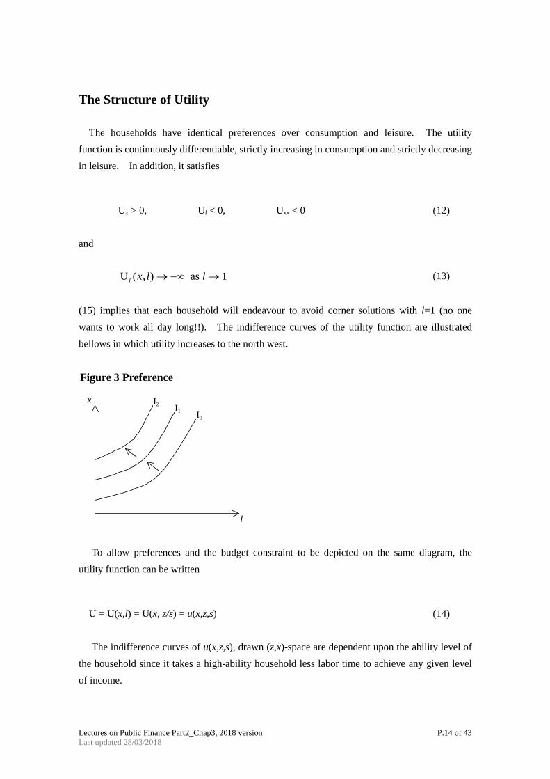
The Structure of Utility The households have identical preferences over consumption and leisure. The utility function is continuously differentiable, strictly increasing in consumption and strictly decreasing in leisure. In addition, it satisfies

Ux > 0, Ul < 0, Uxx < 0 (12) and U as l x l l( , ) → −∞ → 1 (13)

(15) implies that each household will endeavour to avoid corner solutions with l=1 (no one wants to work all day long!!). The indifference curves of the utility function are illustrated bellows in which utility increases to the north west.

Figure 3 Preference

To allow preferences and the budget constraint to be depicted on the same diagram, the

utility function can be written

U = U(x,l) = U(x, z/s) = u(x,z,s) (14)

The indifference curves of u(x,z,s), drawn (z,x)-space are dependent upon the ability level of the household since it takes a high-ability household less labor time to achieve any given level of income.

I0

I1

I2

l

x


In fact, the indifference curves are constructed from those in (l,x)-space by multiplying by the relevant value of s. This construction for the single indifference curve I0 and households of three different ability levels.

Figure 4 Translation of indifference curves.

Agent Monotonicity The utility function (14) satisfies agent monotonicity if –uz/ ux , is a decreasing function of s.

Note that Φ ≡− uu

z

x is the marginal rate of substitution between consumption and pre-tax

income and that agent monotonicity requires ΦΦ

ss

≡ <∂∂

0 .

An equivalent definition of agent monotonicity is that − l UU

l

x is an increasing function of l

as − = −uu

U x z ssU x z s

z

x

l

x

( , )( , )

. Calculating ∂ ∂−

l UU

ll

x and Φs shows

Φsl

xsl UU

l= − −

12 ∂ ∂ (15)

Agent monotonicity is equivalent to the condition that, in the absence of taxation, consumption will increase as the wage rate increases. A sufficient condition for agent monotonicity is that consumption is not inferior, i.e. it does not decrease as lump-sum income increases. The marginal rate of substitution is the gradient of the indifference curve, agent monotonicity

x

l

I0

x

l

I0(S<1)I0(S=1)

I0(S>1)


implies that at any point in (z,x)-space the indifference curve of a household of ability s1 passing through that point is steeper than the curve of a household of ability s2 if s2>s1. Agent monotonicity implies that any two indifference curves of households of different abilities only cross once. In other words, the indifference curve of an s-ability individual through the point (x,z)in consumption-labor space rotates strictly clockwise as s increases. Figure 5

Mirrlees proved a theorem which shows, when the consumption function is a differentiable function of labor supply, agent monotonicity implies that gross income is an increasing function of ability (in other words, if agent monotonicity holds and the implemented tax function has pre-tax income increasing with ability, then the second-order condition for utility maximization must hold). This is important as to identify one’s ability by watching gross income.

Self-selection

Let x(s) and z(s) represent the consumption and income levels that the government intends a household of ability s to choose. The household of ability s will choose (x(s), z(s))provided that this pair generates at least as much utility as any other choice. This condition must apply to all consumption-income pairs and to all households. Formally we can write,

The self-selection constraint is satisfied if u(x(s), z(s), s) ≥ u(x(s’), z(s’), s’) for all s and s’.

In case of linear taxation, it does not need to consider the self-selection constraints since the behavior of the household can be determined as a function of the two parameters that describe the tax function; the lump-sum payment and the marginal rate of tax. In case of non-linear taxation, the self-selection constraints must be included. This is achieved by noting that the satisfaction of the self-selection constraint is equivalent to achieving

s=s2 s=s1

z

x


the minimum of a certain minimization problem. If the sufficient conditions for the minimization are satisfied by the allocation resulting from the tax function, then the self-selection constraint is satisfied. The idea is to induce the more able group to ‘reveal’ that they have a high income, not the reverse. To derive the required minimization problem, let u(s)=u(x(s), z(s), s) represent the maximized level of utility for a consumer of ability s resulting from (10).

0= u(s)-u(x(s), z(s), s) ≤ u(s’)-u(x(s), z(s), s’) (16)

so that s’ =s minimizes u(s’)-u(x(s), z(s), s’). Hence u’(s)=us(x(s), z(s), s). (17) From the definition of u(s) it follows that

uxx’(s) + uzz’(s) = 0 (18)

is equivalent to (17). Condition (17) or (18) is the necessary (the first order) condition for the self-selection constraint to be satisfied. The second-order condition for the self-selection constraint is found from the second derivative of u(s’)-u(x, z, s’) with respect to s’ to be

u’’(s) - uss(x(s), z(s), s) ≥ 0 (19) Again using the definition of u(s), u’’(s) – usxx’(s) + uszz’(s) + uss (20) which gives, by using (19).

usxx’(s) + uszz’(s) ≥ 0 (21) Eliminating x’(s) using (18) provides the final condition


u u uu

z su

z ssz sxz

x

s

x−

= − ≥' ( ) ' ( )Φ 0 (22)

where Φs is the marginal rate of substitution introduced in the discussion of agent monotonicity. With agent monotonicity Φs<0, so that satisfaction of the second-order condition for self-selection is equivalent to z’(s) ≥0. Any tax function that leads to an outcome satisfying (14) and z’(s) ≥0 will therefore satisfy the self-selection constraint.

Characterization of Optimal Tax Function6 It will clearly not be possible to calculate the function without precisely stating the functional forms of utility, production and skill distribution. What will be achieved is the derivation of a set of restrictions that the optimal function must satisfy.

3.7 The General Problem Using the individual demand and supply functions and integrating over the population, it is possible to define total effective labor supply Z, by

Z z s s ds=∞

∫ ( ) ( )γ0

(23)

and aggregate demand, X, where

X x s s ds=∞

∫ ( ) ( )γ0

(24)

The optimal tax function is then chosen to maximize social welfare, where social welfare is given by the Bergson-Samuelson function.

W w u s s ds=∞

∫ ( ( )) ( )γ0

(25)

with W”≤ 0. There are two constraints upon the maximization of (25). The first is that the chosen

6 This part draws from Piketty, T and E. Saez (2013) Chap 5, pp.410-13.


allocation must be productively feasible such that,

X ≤ F(Z) (26)

where F is the production function for the economy. This definition of productive feasibility can incorporate the government revenue requirement,

expressed as a quantity of labor consumed by the government ZG, by noting that (26) can be

written X F Z Z F ZG≤ − = ( ) ( ) .

Denoting the level of revenue required by R(≡ZG), the revenue constraint can be written

[ ]R z s x s s ds≥ −∞

∫ ( ) ( ) ( )γ0

(27)

The second constraint is that it must satisfy the self-selection constraint which has already been discussed.

3.8 Optimal Linear Taxation Basic Model Linear labor income taxation simplifies considerably the exposition but captures the key equity-efficiency trade off. Sheshinski (1972) offered the first modern treatment of optimal linear income taxation following the nonlinear income tax analysis of Mirrlees (1971). Both the derivation and the optimal formulas are also closely related to the more complex nonlinear case. It is therefore pedagogically useful to start with the linear case where the government uses a linear tax at rate 𝝉𝝉 to fund a demogrant R (and additional non-transfer spending E taken as exogenous)7. Summing the Marshallian individual earnings functions zu

i (1− τ, R), we obtain aggregate

earnings which depend upon 𝟏𝟏 − 𝝉𝝉 and R and can be denoted by Zu (1− τ, R) . The government’s budget constraint is 𝑹𝑹 + 𝑬𝑬 = 𝝉𝝉Zu (1− τ, R), which defines implicitly R as a function of 𝝉𝝉 only (as we assume that E is fixed exogenously). Hence, we can express

7 In terms of informational constraints, the government would be constrained to use linear taxation (instead of the

more general nonlinear taxation) if it can only observe the amount of each earnings transaction but cannot observe the identity of individual earners. This could happen for example if the government can only observe the total payroll paid by each employer but cannot observe individual earnings perhaps because there is no identity number system for individuals.


aggregate earnings as a sole function of 𝟏𝟏 − 𝝉𝝉: 𝒁𝒁(𝟏𝟏 − 𝝉𝝉) = Zu (1− τ, R(𝝉𝝉)). The tax revenue function 𝝉𝝉 → 𝝉𝝉𝒁𝒁(𝟏𝟏 − 𝝉𝝉) has an inverted U-shape. It is equal to zero both when 𝝉𝝉 = 𝟎𝟎 (no taxation) and when 𝝉𝝉 = 𝟏𝟏 (complete taxation) as 100% taxation entirely discourages labor supply. This curve is popularly called the Laffer curve although the concept of the revenue

curve has been known since at least Dupuit (1844). Let us denote by 𝒆𝒆 = 𝟏𝟏−𝝉𝝉𝒁𝒁

𝒅𝒅𝒁𝒁𝒅𝒅(𝟏𝟏−𝝉𝝉)

the

elasticity of aggregate earnings with respect to the net-of-tax rate. The tax rate 𝝉𝝉∗

maximizing tax revenue is such that (𝟏𝟏 − 𝝉𝝉) − 𝝉𝝉 𝒅𝒅𝒁𝒁𝒅𝒅(𝟏𝟏−𝝉𝝉)

= 𝟎𝟎 , i.e., 𝝉𝝉𝟏𝟏−𝝉𝝉

𝒆𝒆 = 𝟏𝟏. Hence, we can

express 𝝉𝝉∗ as a sole function of e:

Revenue maximizing linear tax rate: e1

1 *

*=

−ττ or

e+=

11*τ (28)

Let us now consider the maximization of a general social welfare function. The demogrant R

evenly distributed to everybody is equal to 𝝉𝝉𝒁𝒁(𝟏𝟏 − 𝝉𝝉) − 𝑬𝑬 and hence disposable income for individual i is 𝒄𝒄𝒊𝒊 = (𝟏𝟏 − 𝝉𝝉)𝒛𝒛𝒊𝒊 + 𝝉𝝉𝒁𝒁(𝟏𝟏 − 𝝉𝝉) − 𝑬𝑬 (recall that population size is normalized to one). Therefore, the government chooses 𝝉𝝉 to maximize

𝑺𝑺𝑺𝑺𝑺𝑺 = ∫ 𝝎𝝎𝒊𝒊𝑮𝑮[𝒖𝒖𝒊𝒊((𝟏𝟏 − 𝝉𝝉)𝒛𝒛𝒊𝒊 + 𝝉𝝉𝒁𝒁𝒊𝒊 (𝟏𝟏 − 𝝉𝝉) −𝑬𝑬, 𝒛𝒛𝒊𝒊)]𝒅𝒅𝒅𝒅(𝒊𝒊).

Using the envelope theorem from the choice of 𝒛𝒛𝒊𝒊 in the utility maximization problem of individual 𝒊𝒊, the first order condition for the government is simply

𝟎𝟎 = 𝒅𝒅𝑺𝑺𝑺𝑺𝑺𝑺𝒅𝒅𝝉𝝉

= ∫ 𝝎𝝎𝒊𝒊𝑮𝑮′(𝒖𝒖𝒊𝒊)𝒖𝒖𝒄𝒄𝒊𝒊 ∙ 𝒊𝒊 �𝒁𝒁 − 𝒛𝒛𝒊𝒊 − 𝝉𝝉 𝒅𝒅𝒁𝒁𝒅𝒅(𝟏𝟏−𝝉𝝉)

� 𝒅𝒅𝒅𝒅(𝒊𝒊),

The first term in the square brackets 𝒁𝒁 − 𝒛𝒛𝒊𝒊 reflects the mechanical offect of increasing taxes (and the demogrant) absent any behavioral response. This effect is positive when individual

income 𝒛𝒛𝒊𝒊 is less than average income 𝒁𝒁. The second term −𝝉𝝉𝒅𝒅𝒁𝒁 𝒅𝒅(𝟏𝟏 − 𝝉𝝉)⁄ reflects the efficiency cost of increasing taxes due to the aggregate behavioral response. This is an efficiency cost because such behavioral responses have no first order positive welfare effect on individuals but have a first order negative effect on tax revenue. Introducing the aggregate elasticity 𝒆𝒆 and the “normalized” social marginal welfare weight 𝒈𝒈𝒊𝒊 = 𝝎𝝎𝒊𝒊𝑮𝑮′(𝒖𝒖𝒊𝒊)𝒖𝒖𝒄𝒄𝒊𝒊 ∫𝝎𝝎𝒊𝒊𝑮𝑮′(𝒖𝒖𝒊𝒊)𝒖𝒖𝒄𝒄𝒊𝒊⁄ 𝒅𝒅𝒅𝒅(𝒋𝒋), we can rewrite the forst order condition as:


𝒁𝒁 ∙ �𝟏𝟏 − 𝝉𝝉𝟏𝟏−𝝉𝝉

𝒆𝒆� = ∫ 𝒈𝒈𝒊𝒊𝒛𝒛𝒊𝒊𝒅𝒅𝒅𝒅(𝒊𝒊)𝒊𝒊 .

Hence, we have the following optimal linear income tax formula

Optimal linear tax rate: 𝝉𝝉 = 𝟏𝟏−𝒈𝒈�𝟏𝟏−𝒈𝒈�+𝒆𝒆

with 𝒈𝒈� = ∫𝒈𝒈𝒊𝒊𝒛𝒛𝒊𝒊𝒅𝒅𝒅𝒅(𝒊𝒊)𝒁𝒁

(29)

𝒈𝒈� is the average “normalized” social marginal welfare weight weighted by pre-tax incomes 𝒛𝒛𝒊𝒊 ∙𝒈𝒈� is also the ratio of the average income weighted by individual social welfare weights 𝒈𝒈𝒊𝒊 to the actual average income 𝒁𝒁 . Hence, 𝒈𝒈� measures where social welfare weights are concentrated on average over the distribution of earnings. An alternative form for formula (29) often presented in the literature takes the form 𝝉𝝉 = −𝒄𝒄𝒄𝒄𝒅𝒅(𝒈𝒈𝒊𝒊, 𝒛𝒛𝒊𝒊 𝒁𝒁⁄ ) [−𝒄𝒄𝒄𝒄𝒅𝒅(⁄ 𝒈𝒈𝒊𝒊, 𝒛𝒛𝒊𝒊 𝒁𝒁⁄ ) +𝒆𝒆] where 𝒄𝒄𝒄𝒄𝒅𝒅(𝒈𝒈𝒊𝒊, 𝒛𝒛𝒊𝒊 𝒁𝒁⁄ ) is the covariance between social marginal welfare weights 𝒈𝒈𝒊𝒊 and normalized earnings 𝒛𝒛𝒊𝒊 𝒁𝒁⁄ . As long as the correlation between 𝒈𝒈𝒊𝒊 and 𝒛𝒛𝒊𝒊 is negative, i.e., those with higher incomes have lower social marginal welfare weights, the optimum 𝝉𝝉 is positive. Five points are worth noting about formula (29). 1) The optimal tax rate decreases with the aggregate elasticity 𝒆𝒆. This elasticity is a mix of

substitution and income effects as an increase in the tax rate 𝝉𝝉 is associated with an increase in the demogrant 𝑹𝑹 = 𝝉𝝉𝒁𝒁(𝟏𝟏 − 𝝉𝝉) − 𝑬𝑬 . Formally, one can show that 𝒆𝒆 =

[𝒆𝒆�𝒖𝒖 − 𝜼𝜼�]/[𝟏𝟏 − 𝜼𝜼�𝝉𝝉/(𝟏𝟏 − 𝝉𝝉)] where 𝒆𝒆�𝒖𝒖 = 𝟏𝟏−𝝉𝝉𝒁𝒁𝒖𝒖

𝝏𝝏𝒛𝒛𝝏𝝏(𝟏𝟏−𝝉𝝉)

is the average of the individual

uncompensated elasticities 𝒆𝒆𝒖𝒖𝒊𝒊 weighted by income 𝒛𝒛𝒊𝒊 and 𝜼𝜼� = (𝟏𝟏 − 𝝉𝝉) 𝝏𝝏𝒁𝒁𝒖𝒖𝝏𝝏𝑹𝑹

is the

unweighted average of individual income effects 𝜼𝜼𝒊𝒊. 8 This allows us to rewrite the optimal tax formula (29) in a slightly more structural for as 𝝉𝝉 =(𝟏𝟏 − 𝒈𝒈�) (𝟏𝟏 − 𝒈𝒈� − 𝒈𝒈� ∙ 𝜼𝜼� + 𝒆𝒆�𝒖𝒖)⁄ . When the tax rate maximizes tax revenue, we have 𝝉𝝉 = 𝟏𝟏 (𝟏𝟏 + 𝒆𝒆)⁄ and then 𝒆𝒆 = 𝒆𝒆�𝒖𝒖 is a pure uncompensated elasticity (as the tax rate does not raise any extra revenue at the margin). When the tax rate is zero, 𝒆𝒆 is conceptually close to a compensated elasticity as taxes raised are fully rebated with no efficiency loss9.

2) The optimal tax rate naturally decreases with 𝒈𝒈� which measures the redistributive tastes of

8 To see this, recall that 𝑍𝑍(1 − 𝜏𝜏) = 𝑍𝑍𝑢𝑢(1 − 𝜏𝜏, 𝜏𝜏𝑍𝑍(1 − 𝜏𝜏) − 𝐸𝐸) so that 𝑑𝑑𝑑𝑑

𝑑𝑑(1−𝜏𝜏)�1 − 𝜏𝜏 𝜕𝜕𝑑𝑑𝑢𝑢

𝜕𝜕𝜕𝜕� = 𝜕𝜕𝑑𝑑𝑢𝑢

𝜕𝜕(1−𝜏𝜏)− 𝑍𝑍 𝜕𝜕𝑑𝑑𝑢𝑢

𝜕𝜕𝜕𝜕.

9 It is not exactly a compensated elasticity as ��𝑒𝑢𝑢 is income weighted while ��𝜂 is not.


the government. In the extreme case where the government does not value redistribution at all, 𝒈𝒈𝒊𝒊 ≡ 𝟏𝟏 and hence 𝒈𝒈� = 𝟏𝟏 and 𝝉𝝉 = 𝟎𝟎 is optimal10. In the polar opposite case where the government is Rawlsian and maximizes the lump sum demogrant (assuming the worst-off individual has zero earnings), then 𝒈𝒈� = 𝟎𝟎 and 𝝉𝝉 = 𝟏𝟏/(𝟏𝟏 + 𝒆𝒆), which is the revenue maximizing tax rate from Eq.(28). As mentioned above, in that case 𝒆𝒆 = 𝒆𝒆�𝒖𝒖 is an uncompensated elasticity.

3) For a given profile of social welfare weights (or for a given degree of concavity of the utility function in the homogeneous utilitarian case), the higher the pre-tax inequality at a given 𝝉𝝉, the lower 𝒈𝒈�, and hence the higher the optimal tax rate. If there is no inequality,

then 𝒈𝒈� = 𝟏𝟏 and 𝝉𝝉 = 𝟎𝟎 with a lump-sum tax –𝑹𝑹 = 𝑬𝑬 is optimal. If inequality is maximal, i.e., nobody earns anything except for a single person who earns everything and has a social marginal welfare weight of zero, then 𝝉𝝉 = 𝟏𝟏/(𝟏𝟏 + 𝒆𝒆), again equal to the revenue maximizing tax rate.

4) It is important to note that, as is usual in optimal tax theory, formula (29) is an implicit formula for 𝝉𝝉 as both 𝒆𝒆 and aspecially 𝒈𝒈� vary with 𝝉𝝉. Under a standard utilitarian social welfare criterion with concave utility of consumption, 𝒈𝒈� increases with 𝝉𝝉 as the need for redistribution (i.e., the variation of the 𝒈𝒈𝒊𝒊 with 𝒛𝒛𝒊𝒊) decreases with the level of taxation 𝝉𝝉. This ensures that formla (29) generates a unique equilibrium for 𝝉𝝉.

5) Formula (29) can also be used to assess tax reform. Starting from the current 𝝉𝝉, the current estimated elasticity 𝒆𝒆, and the current welfare weight parameter 𝒈𝒈�, if 𝝉𝝉 < (𝟏𝟏 −𝒈𝒈�)/(𝟏𝟏 − 𝒈𝒈� + 𝒆𝒆) then increasing 𝝉𝝉 increases social welfare (and conversely). The tax reform approach has the advantage that it does not require knowing how 𝒆𝒆 and 𝒈𝒈� change with 𝝉𝝉, since it only considers local variations. Generality of the Formula. The optimal linear tax formula is very general as it applies to many alternative models for the income generating process. All that matters is the aggregate elasticity 𝒆𝒆 and how the government sets normalized marginal welfare weights 𝒈𝒈𝒊𝒊. First, if the population is discrete, the same derivation and formula obviously apply. Second, if labor supply responses are (partly or fully) along the extensive margin, the same formula applies. Third, the same formula also applies in the long run when educational and human capital decisions are potentially affected by the tax rate as those responses are reflected in the long-run aggregate elasticity 𝒆𝒆 (see e.g., Best & Kleven, 2012).11

10 This assumes that a lump sum tax 𝐸𝐸 is feasible to fund government spending. If lump sum taxes are not

feasible, for example because it is impossible to set taxes higher than earnings at the bottom, then the optimal tax in that case is the smallest 𝜏𝜏 such that 𝜏𝜏𝑍𝑍(1 − 𝜏𝜏) = 𝐸𝐸, i.e., the level of tax required to fund government spending 𝐸𝐸.

11 Naturally, such long-run responses are challenging to estimate empirically as short-tem comparisons around a tax reform cannot capture them.


3.9 Optimal Nonlinear Taxation12 Formally, the optimal nonlinear tax problem is easy to pose. It is the same as the linear tax problem except that the government can now choose any nonlinear tax schedule 𝑻𝑻(𝒛𝒛) instead of a single linear tax rate 𝝉𝝉 with a demogrant 𝑹𝑹. Therefore, the government chooses 𝑻𝑻(𝒛𝒛) to maximize.

𝑺𝑺𝑺𝑺𝑺𝑺 = ∫ 𝝎𝝎𝒊𝒊𝑮𝑮(𝒖𝒖𝒊𝒊(𝒛𝒛𝒊𝒊 − 𝑻𝑻(𝒛𝒛𝒊𝒊),𝒛𝒛𝒊𝒊)𝒅𝒅𝒅𝒅(𝒊𝒊)𝒊𝒊 . subject to ∫ 𝑻𝑻(𝒛𝒛𝒊𝒊)𝒅𝒅𝒅𝒅(𝒊𝒊)𝒊𝒊 ≥ 𝑬𝑬(𝒑𝒑),

and the fact that 𝒛𝒛𝒊𝒊 is chosen by individual 𝒊𝒊 to maximize her utility 𝒖𝒖𝒊𝒊(𝒛𝒛𝒊𝒊 − 𝑻𝑻(𝒛𝒛𝒊𝒊),𝒛𝒛𝒊𝒊). Note that transfers and taxes are fully integrated. Those with no earnings receive a transfer

–𝑻𝑻(𝟎𝟎). We start the analysis with the optimal top tax rate. Next, we derive the optimal marginal tax rate at any income level 𝒛𝒛. Finally, we focus on the bottom of the income distribution to discuss the optimal profile of transfers. In this chapter, we purposefully focus on intuitive derivations using small reforms around the optimum. This allows us to understand the key economic mechanisms and obtain formulas directly expressed in terms of estimable “sufficient statistics” (Chetty, 2009a; Saez, 2001). Hence, we will omit discussions of technical issues about regularity conditions needed for the optimal tax formulas13. Figure 6 Optimal Top Tax Rate Derivation

z

Disposable Income c=z-T(z) Top bracket: slope 1-τ above z*

Mechanical tax increase: dτ[z-z*]

Behavioral response tax loss: τdz=dτez τ/(1-τ)

Pre-tax income z z* 0

z*-T(z*)

Reform: slope 1-τ-dτ above z*

The figure adapted from Diamond and Saez (2011), depicts the derivation of the optimal top tax rate 𝝉𝝉 = 𝟏𝟏/(𝟏𝟏 + ae) by considering a small reform around the optimum which increases the

12 This part draws from Piketty, T and E. Saez (2013) Chap 5, pp.421-25. 13 The optimal income tax theory following Mirrlees (1971) has devoted substantial effort studying those issues

thoroughly (see e.g., Mirrlees (1976, 1986, chap. 24) for extensive surveys). The formal derivations are gathered in the appendix.


top marginal tax rate 𝝉𝝉 by 𝒅𝒅𝛕𝛕 above z*. A taxpayer with income z mechanically pays 𝒅𝒅𝝉𝝉[𝒛𝒛 − 𝒛𝒛∗] extra taxes but, by definition of the elasticity e of earnings with respect to the net-of-tax rate 𝟏𝟏 − 𝝉𝝉, also reduces his income by 𝒅𝒅𝒛𝒛 = −𝒅𝒅𝝉𝝉𝒆𝒆𝒛𝒛(𝟏𝟏 − 𝝉𝝉) leading to a loss in tax revenue equal to 𝒅𝒅𝝉𝝉𝒆𝒆𝒛𝒛𝝉𝝉(𝟏𝟏 − 𝝉𝝉). Summing across all top bracket taxpayers and denoting by z the average income above 𝒛𝒛∗ and 𝒂𝒂 = 𝒛𝒛/(𝒛𝒛 − 𝒛𝒛∗), we obtain the revenue maximizing tax rate 𝝉𝝉 = 𝟏𝟏/(𝟏𝟏 + 𝒂𝒂𝒆𝒆). This is the optimum tax rate when the government sets zero marginal welfare weights on top income earners. 3.9.1 Optimal Top Tax Rate The taxation of high income earners is a very important aspect of the tax policy debate. Initial progressive income tax systems were typically limited to the top of the distribution. Today, because of large increases in income concentration in a number of countries and particularly the United States (Piketty and Saez, 2003), the level of taxation of top incomes (e.g., the top 1%) matters not only for symbolic equity reasons but also for quantitatively for revenue raising needs. Standard Model Let us assume that the top tax rate above a fixed income level 𝒛𝒛∗ is constant and equal to 𝝉𝝉 as illustarated on Figure 6. Let us assume that a fraction q of individuals are in the top bracket. To obtain the optimal 𝝉𝝉, we consider a small variation 𝒅𝒅𝝉𝝉 as depicted on Figure 6. Individual i earning 𝒛𝒛𝒊𝒊 above 𝒛𝒛∗, mechanically pays [𝒛𝒛𝒊𝒊 − 𝒛𝒛∗]𝒅𝒅𝛕𝛕 extra in taxes. This extra tax payment creates a social welfare loss (expressed in terms of government public funds) equal to −𝒈𝒈𝒊𝒊 ∙[𝒛𝒛𝒊𝒊 − 𝒛𝒛∗]𝒅𝒅𝛕𝛕 where 𝒈𝒈𝒊𝒊 = 𝝎𝝎𝒊𝒊𝑮𝑮′(𝒖𝒖𝒊𝒊)𝒖𝒖𝒄𝒄𝒊𝒊/𝒑𝒑 is the social marginal welfare weight on individual i14. Finally, the tax change triggers a behavioral response 𝒅𝒅𝒛𝒛𝒊𝒊 leading to an additional change in tax 𝝉𝝉𝒅𝒅𝒛𝒛𝒊𝒊. Using the elasticity of reported income 𝒛𝒛𝒊𝒊 with respect to the net-of tax rate 𝟏𝟏 − 𝝉𝝉, we have 𝒅𝒅𝒛𝒛𝒊𝒊 = −𝒆𝒆𝒊𝒊𝒛𝒛𝒊𝒊𝒅𝒅𝛕𝛕/(𝟏𝟏 − 𝝉𝝉). Hence, the net effect of the small reform on individual 𝒊𝒊 is:

�(𝟏𝟏 − 𝒈𝒈𝒊𝒊)(𝒛𝒛𝒊𝒊 − 𝒛𝒛∗)− 𝒆𝒆𝒊𝒊𝒛𝒛𝒊𝒊 𝝉𝝉𝟏𝟏−𝝉𝝉

� 𝒅𝒅𝛕𝛕.

To obtain the total effect on social welfare, we simply aggregate the welfare effects across all top bracket taxpayers so that we have:

14 Because the individual chooses 𝑧𝑧𝑖𝑖 to maximize utility, the money-metric welfare effect of the reform on

individual i is given by [𝑧𝑧𝑖𝑖 − 𝑧𝑧∗]𝑑𝑑τ using the standard envelope theorem argument.


𝒅𝒅𝑺𝑺𝑺𝑺𝑺𝑺 �(𝟏𝟏 − 𝒈𝒈)(𝒛𝒛 − 𝒛𝒛∗) − 𝒆𝒆𝒛𝒛 𝝉𝝉𝟏𝟏−𝝉𝝉

� 𝒒𝒒𝒅𝒅𝛕𝛕,

where 𝒒𝒒 is the fraction of individuals in the top bracket, 𝒛𝒛 is average income in the top bracket, 𝒈𝒈 is the average social marginal welfare weight (weighted by income in the top bracket 𝒛𝒛𝒊𝒊 − 𝒛𝒛∗) of top bracket individuals, and 𝒆𝒆 is the average elasticity (weighted by income 𝒛𝒛𝒊𝒊) of top bracket individuals. We can introduce the tail-parameter 𝒂𝒂 = 𝒛𝒛/(𝒛𝒛 − 𝒛𝒛∗) to rewrite 𝒅𝒅𝑺𝑺𝑺𝑺𝑺𝑺 as

𝒅𝒅𝑺𝑺𝑺𝑺𝑺𝑺 �𝟏𝟏 − 𝒈𝒈 − 𝒂𝒂 ∙ 𝒆𝒆 𝝉𝝉𝟏𝟏−𝝉𝝉

� (𝒛𝒛 − 𝒛𝒛∗)𝒒𝒒𝒅𝒅𝛕𝛕.

At the optimum, 𝒅𝒅𝑺𝑺𝑺𝑺𝑺𝑺 = 𝟎𝟎, leading to the following optimal top rate formula.

Optimal top tax rate: 𝝉𝝉 = 𝟏𝟏−𝒈𝒈𝟏𝟏−𝐠𝐠+𝒂𝒂∙𝒆𝒆

. (30)

Formula (30) expresses the optimal top tax rate in terms of three parameters: a parameter 𝒈𝒈 for social preferences, a parameter 𝒆𝒆 for behavioral responses to taxes, and a parameter 𝒂𝒂 for the shape of the income distribution15. Five points are worth noting about formula (30).

First, the optimal taxrate decreases with 𝒈𝒈, the social marginal welfare weight on top bracket earners. In the limit case where society does not put any value on the marginal consumption of top earners, the formula simplifies to 𝝉𝝉 = 𝟏𝟏/(𝟏𝟏 + 𝒂𝒂 ∙ 𝒆𝒆) which is the revenue maximizing top tax rate. A utilitarian social welfare criterion with marginal utility of consumption declining to zero, the most commonly used specification in optimal tax models following Mirrlees (1971), has the implication that 𝒈𝒈 converges to zero when 𝒛𝒛∗ grows to infinity.

Second, the optimal tax rate decreases with the elasticity 𝒆𝒆 as a higher elasticity leads to larger efficiency costs. Note that this elasticity is a mixture of substitution and income effects as an increase in the top tax rate generates both substitution and income effects16.

Importantly, for a given compensated elasticity, the presence of income effects increases the optimal top tax rate as raising the tax rate reduces disposable income and hence increases labor

15 Note that the derivation and formula are virtually the same as for the optimal linear rate by simply multiplying 𝑒𝑒

by the factor 𝑎𝑎 > 1. Indeed, when 𝑧𝑧∗ = 0, 𝑎𝑎 = 𝑧𝑧/(𝑧𝑧 − 𝑧𝑧∗) = 1 and the problem boils down to the optimal linear tax problem.

16 Saez (2001) provides a decomposition and shows that 𝑒𝑒 = ��𝑒𝑢𝑢 + ��𝜂 ∙ (𝑎𝑎 − 1)/𝑎𝑎 with ��𝑒𝑢𝑢 the average (income weighted) uncompensated elasticity and ��𝜂 the (unweighted) average income effect.


supply. Figure 7

Empirical Pareto coefficients in the United States, 2005. The figure, from Diamond and Saez (2011), depicits in solid line the ratio 𝒂𝒂 = 𝒛𝒛𝒎𝒎/(𝒛𝒛𝒎𝒎 − 𝒛𝒛∗) with 𝒛𝒛∗ ranging from $0 to $1,000,000 annual income and 𝒛𝒛𝒎𝒎 the average income above 𝒛𝒛∗ using US tax return micro data for 2005. Income is defined as Adjusted Gross Income reported on tax returns and is expressed in current 2005 dollars. Vertical lines depict the 90th percentile ($99,200) and 99th percentile ($350,500) nominal thresholds as of 2005. The ratio 𝒂𝒂 is equal to one at 𝒛𝒛∗ = 𝟎𝟎, and is almost constant above the 99th percentile and slightly below 1.5, showing that the top of the distribution is extremely well approximated by a Pareto distribution for purposes of implementing the optimal top tax rate formula 𝝉𝝉 = 𝟏𝟏/(𝟏𝟏 +𝒂𝒂𝒆𝒆). Denoting by 𝒉𝒉(𝒛𝒛) the density and by 𝑯𝑯(𝒛𝒛) the cdf of the income distribution, the figure also displays in dotted line the ratio 𝜶𝜶(𝒛𝒛∗) = 𝒛𝒛∗𝒉𝒉(𝒛𝒛∗)/(𝟏𝟏 − 𝑯𝑯(𝒛𝒛∗)) which is also approximately constant, around 1.5, above the top percentile. A decreasing (or constant) 𝜶𝜶(𝒛𝒛) combined with a decreasing 𝒈𝒈+(𝒛𝒛) and a constant 𝒆𝒆(𝒛𝒛) implies that the optimal marginal tax rate 𝑻𝑻′(𝒛𝒛) = [𝟏𝟏 − 𝒈𝒈+(𝒛𝒛)]/[𝟏𝟏 − 𝒈𝒈+(𝒛𝒛) + 𝜶𝜶(𝒛𝒛)𝒆𝒆(𝒛𝒛)] increases with 𝒛𝒛.

Third, the optimal tax rate decreases with the parameter 𝒂𝒂 ≥ 𝟏𝟏 which measures the thinness

of the top tail of the income distribution. Empirically, 𝒂𝒂 = 𝒛𝒛/(𝒛𝒛 − 𝒛𝒛∗) is almost constant as 𝒛𝒛∗ varies in the top tail of the earnings distribution. Figure 7 depicts 𝒂𝒂 (as a function of 𝒛𝒛∗) for the case of the US pre-tax income distribution and shows that it is extremely stable above 𝒛𝒛∗ = $𝟒𝟒𝟎𝟎𝟎𝟎,𝟎𝟎𝟎𝟎𝟎𝟎, approximately the top 1% threshold17. This is due to the well-known fact – since at least Pareto (1896) – that the top tail is very closely approximated by a Pareto distribution18.

Forth, and related, the formula shows the limited relevance of the zero-top tax rate result. Formally, 𝒛𝒛/𝒛𝒛∗ reaches 1 when 𝒛𝒛∗ reaches the level of income of the single highest income 17 This graph is taken from Diamond and Saez (2011) who use the 2005 distribution of total pre-tax family income

(including capital income and realized capital gains) based on tax return data. 18 A Pareto distribution with parameter 𝑎𝑎 has a distribution of the form 𝐻𝐻(𝑧𝑧) = 1 − 𝑘𝑘/𝑧𝑧𝑎𝑎 and density ℎ(𝑧𝑧) =

𝑘𝑘𝑎𝑎/𝑧𝑧1+𝑎𝑎 (with 𝑘𝑘 a constant parameter). For any 𝑧𝑧∗, the average income above 𝑧𝑧∗ is equal to 𝑧𝑧∗ ∙ 𝑎𝑎(𝑎𝑎 − 1).

2

2.5

1.5

1

1000000 800000 600000 400000 200000 0

𝑎𝑎 = 𝑧𝑧𝑚𝑚/(𝑧𝑧𝑚𝑚 − 𝑧𝑧∗) with 𝑧𝑧𝑚𝑚 = 𝐸𝐸(𝑧𝑧|𝑧𝑧 > 𝑧𝑧∗) alpha = 𝑧𝑧∗ℎ(𝑧𝑧∗)/(1 − 𝐻𝐻(𝑧𝑧∗))


earner, in which case 𝒂𝒂 = 𝒛𝒛/(𝒛𝒛 − 𝒛𝒛∗) is infinite and indeed 𝝉𝝉 = 𝟎𝟎, which is the famous zero-top rate result first demonstrated by Sadka (1976) and Seade (1977). However, notice that this result applies only to the very top income earner. Its lack of wider applicability can be verified empirically using distributional income tax statistics as we did in Figure 7 (see Saez, 2001 for an extensive analysis). Furthermore, under the reasonable assumption that the level of top earnings is not known in advance and where potential earnings are drawn randomly from an underlying Pareto distribution then, with the budget constraint satisfied in expectation, formula (30) remains the natural optimum tax rate (Diamond & Saez, 2011). This finding implies that the zero-top rate result and its corollary that marginal tax rates should decline at the top have no policy relevance.

Fifth, the optimal top tax rate formula is fairly general and applies equally to populations with heterogeneous preferences discreate populations, or continuous populations. Although the optimal formla does not require the strong homogeneity assumptions of the Mirrlees (1971) problem, it is also the asymptotic limit of the optimal marginal tax rate of the fully nonlinear tax problem of Mirrlees (1971).

3.10 Numerical Results19 To generate numerical results, Mirrlees (1971) assumed that the social welfare function took the form

0 , )(

0 , )(1

0

0

==

=

∫

∫∞

−∞

vdssU

v>dssev

w vU

γ

γ (31)

Higher values of v represent greater concern for equity, with v=0 representing the utilitarian case.

The individual utility function was the Cobb-Douglas,

U x l= + −log log( )1 (32)

and the skill distribution is log-normal,

19 This part draws from Myles (1955) Chap 2, pp.156-9.


( )

+−=

2)1log(exp1)(

2ss

sγ (33)

With a standard deviation σ (=0.39 from Lydall (1968)). An implicit assumption is that the skill distribution can be inferred directly from an observed income distribution. Table 3 Optimal Tax Schedule

Income Consumption Average tax (%) Marginal tax (%) (a) zG=0.013, v=0,σ=0.39

0.00 0.03 --- 23 0.05 0.07 -34 26 0.10 0.10 -5 24 0.20 0.18 9 21 0.30 0.26 13 19 0.40 0.34 14 18 0.50 0.43 15 16

(b) zG=0.003, v=1,σ=0.39 0.00 0.05 --- 30 0.05 0.08 -66 34 0.10 0.12 -34 32 0.20 0.19 7 28 0.30 0.26 13 25 0.40 0.34 16 22 0.50 0.41 17 20

(c) zG=0.013, v=1,σ=1 0.00 0.10 --- 50 0.10 0.15 -50 58 0.25 0.20 20 60 0.50 0.30 40 59 1.00 0.52 48 57 1.50 0.73 51 54 2.00 0.97 51 52 3.00 1.47 51 49

Source: Mirrlees (1971)

The most important feature of the first two panels (a) and (b) in Table 3 is the low marginal rates of tax, with the maximal rate being only 34%. There is also limited deviation in these rates. The marginal rates become lower at high incomes but do not reach 0 because the skill distribution is unbounded. The average rate of tax is negative for low incomes so that low-income consumers are receiving an income supplement from the government.

The panel (c) of Table 3 show the effect of increasing the dispersion of skills (changing standard deviation from 0.39 to 1.00). This raises the marginal tax rates but there remain fairly constant across the income range. Kanbur and Tuomala (1994) find that an increased dispersion of skills raises the marginal tax rate at each income level and that it also has the effect of moving the maximum tax rate up the income range, so that the marginal tax rate is increasing over the majority of households.


Atkinson (1975) considered the effect of changing the social welfare function to the extreme maxi-min form,

w=min{U} (34)

From the above table, it can be seen that increased concern for equity, v going from 0 to 1, increased the optimal marginal tax rates. The natural question is “can strong equity considerations such as maxi-min SWF lead to high marginal rates?”. The result is given the below table. The maxi-min criterion leads to generally higher taxes. However they are again highest at low incomes and then decline. Absolute rate is lower than expected in all cases. Table 4 Optimal tax Schedule: Utilitarian vs. Maxi-min

Utilitarian Maxi-min Level of s Average rate (%) Marginal rate (%) Average rate (%) Marginal rate (%)

Median (50%) 6 21 10 52 Top decile (10%) 14 20 28 34 Top percentile (1%) 16 17 28 26 Source: Atkinson and Stiglitz (1980, Table 13-3, p.421)

3.12 Voting over a Flat Tax20 Having identified the properties of the optimal tax structure, we now consider the tax system that emerges from the political process. To do this, we consider people voting over tax schedules that have some degree of redistribution. Because it is difficult to model voting on nonlinear tax schemes given the high dimensionality of the problem, we will restrict attention to a linear tax structure as originally proposed by Romer (1975). We specify the model further with quasi-linear preferences to avoid unnecessary complications and to simplify the analysis of the voting equilibrium. Assume, as before, that individuals differ only in their level of skill. We assume that skills are distributed in the population according to a cumulative distribution function )(sF that is known to everyone, with mean skill s and median ms . Individuals work and consume.

They also vote on a linear tax scheme that pays a lumpsum benefit b to each individual financed by a proportional income tax at rate t . The individual utility function has the quasi-linear form

2

21,

−=

szx

szxu , (35)

20 This part is drawn from Hindriks and Myles (2006) Chapter 15, pp.503-5.


and the individual budget constraint is bztx +−= ]1[ . (36)

It is easy to verify that in this simple model the optimal income choice of a consumer with skill level s is 2]1[)( stsz −= . (37) The quasi-linear preferences imply that there is no income effect on labor supply (i.e., )(sz is

independent of the lump-sum benefit b ). This simplifies the expression of the tax distortion and makes the analysis of the voting equilibrium easier. Less surprisingly a higher tax rate induces taxpayers to work less and earn less income. The lump-sum transfer b is constrained by the government budget balance condition )(]1[))(( 2sEttsztEb −== , (38) where )(⋅E is the mathematical expectation, and we used the optimal income choice to derive

the second equality. This constraint says that the lump-sum benefit paid to each individual must be equal to the expected tax payment ))(( sztE . This expression is termed the

Dupuit-Laffer curve and describes tax revenue as a function of the tax rate. In this simple model the Dupuit-Laffer curve is bell-shaped with a peak at 2/1=t and no tax collected at the ends 0=t and 1=t . We can now derive individual preferences over tax schedules by substituting (36) and (37) into (35). After re-arrangement (indirect) utility can be written

22]1[21),,( stbsbtv −+= . (39)

Taking the total differential of (39) gives dtstdbdv 2]1[ −−= . (40) so that along an indifference curve where 0=dv ,


2]1[ stdtdb

−= . (41)

It can be seen from this that for given t , the indifference curve becomes steeper in ),( bt

space as s increases. This monotonicity is a consequence of the single-crossing property of the indifference curves. The single-crossing property is a sufficient condition for the Median Voter Theorem to apply. It follows that there is only one tax policy that can result from majority voting: it is the policy preferred by the median voter (half the voters are poorer than the median and prefer higher tax rates, and the other half are richer and prefer lower tax rates). Letting mt be the tax rate preferred by the median voter, then we have mt implicitly defined

by the solution to the first-order condition for maximizing the median voter’s utility. We differentiate (39) with respect to t , taking into account the government budget constraint (38) to obtain

22 ]1[)(]21[ stsEttv

−−−=∂∂ . (42)

Setting this expression equal to zero for the median skill level ms yields the tax rate preferred

by the median voter

22

22

)(2)(

m

mm ssE

ssEt

−

−= , (43)

or, using the optimal income choice (37),

m

mm zzE

zzEt

−

−=

)(2)( . (44)

This simple model predicts that the political equilibrium tax rate is determined by the position of the median voter in the income distribution. The greater is income inequality as measured by the distance between median and mean income, the higher the tax rate. If the median voter is relatively worse off, with income well below the mean income, then equilibrium redistribution is large. In practice, the income distribution has a median income below the mean income, so a majority of voters would favor redistribution through proportional income taxation. More general utility functions would also predict that the extent of this redistribution decreases with the elasticity of labor supply.


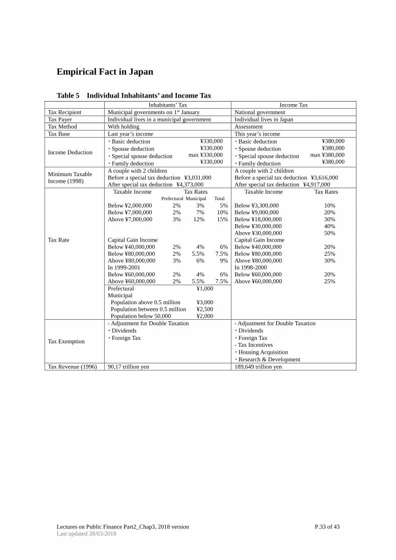
Empirical Fact in Japan Table 5 Individual Inhabitants’ and Income Tax

Inhabitants’ Tax Income Tax Tax Recipient Municipal governments on 1st January National government Tax Payer Individual lives in a municipal government Individual lives in Japan Tax Method With holding Assessment Tax Base Last year’s income This year’s income

Income Deduction

・ Basic deduction ・ Spouse deduction ・ Special spouse deduction ・ Family deduction

¥330,000 ¥330,000

max ¥330,000 ¥330,000

・ Basic deduction ・ Spouse deduction ・ Special spouse deduction ・ Family deduction

¥380,000 ¥380,000

max ¥380,000 ¥380,000

Minimum Taxable Income (1998)

A couple with 2 children Before a special tax deduction ¥3,031,000 After special tax deduction ¥4,373,000

A couple with 2 children Before a special tax deduction ¥3,616,000 After special tax deduction ¥4,917,000

Taxable Income Tax Rates Taxable Income Tax Rates Prefectural Municipal Total Below ¥2,000,000

Below ¥7,000,000 Above ¥7,000,000

2% 2% 3%

3% 7%

12%

5% 10% 15%

Below ¥3,300,000 Below ¥9,000,000 Below ¥18,000,000 Below ¥30,000,000 Above ¥30,000,000

10% 20% 30% 40% 50%

Tax Rate Capital Gain Income Capital Gain Income Below ¥40,000,000

Below ¥80,000,000 Above ¥80,000,000

2% 2% 3%

4% 5.5%

6%

6% 7.5%

9%

Below ¥40,000,000 Below ¥80,000,000 Above ¥80,000,000

20% 25% 30%

In 1999-2001 In 1998-2000 Below ¥60,000,000

Above ¥60,000,000 2% 2%

4% 5.5%

6% 7.5%

Below ¥60,000,000 Above ¥60,000,000

20% 25%

Prefectural ¥1,000 Municipal

Population above 0.5 million Population between 0.5 million Population below 50,000

¥3,000 ¥2,500 ¥2,000

Tax Exemption

- Adjustment for Double Taxation ・ Dividends ・ Foreign Tax

- Adjustment for Double Taxation ・ Dividends ・ Foreign Tax - Tax Incentives ・ Housing Acquisition ・ Research & Development

Tax Revenue (1996) 90,17 trillion yen 189,649 trillion yen


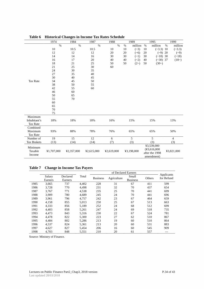
Table 6 Historical Changes in Income Tax Rates Schedule 1974 1984 1987 1988 1989 1995 1999 % % % % % million % million % million

Tax Rate

10 12 14 16 18 21 24 27 30 34 38 42 46 50 55 60 65 70 75

10.5 12 14 17 21 25 30 35 40 45 50 55 60 65 70

10.5 12 16 20 25 30 35 40 45 50 55 60

10 20 30 40 50 60

10 20 30 40 50

(~3) (~6) (~1) (~2) (2~)

10 20 30 40 50

(~3.3) (~9)

(~18) (~30) (30~)

10 20 30 37

(~3.3) (~9)

(~18) (18~)

Maximum Inhabitant’s

Tax Rate 18% 18% 18% 16% 15% 15% 13%

Combined Maximum Tax Rate

93% 88% 78% 76% 65% 65% 50%

Number of Tax Brakets

19 (13)

15 (14)

12 (14)

6 (7)

5 (3)

5 (3)

4 (3)

Minimum Taxable Income

¥1,707,000 ¥2,357,000 ¥2,615,000 ¥2,619,000 ¥3,198,000

¥3,539,000 (¥3,616,000

after the 1998 amendment)

¥3,821,000

Table 7 Change in Income Tax Payers

Total of Declared Earners Applicants

for Refund Salary Earners

Declared Earners Business Agriculture Small

Business Others

1985 3,665 737 4,402 228 31 67 411 599 1986 3,728 770 4,498 231 32 70 437 654 1987 3,767 771 4,538 235 25 70 441 699 1988 3,909 780 4,689 245 24 70 441 696 1989 3,961 796 4,757 242 23 67 464 659 1990 4,158 855 5,013 250 25 67 513 663 1991 4,333 856 5,189 252 24 68 512 699 1992 4,403 858 5,261 247 24 69 518 735 1993 4,473 843 5,316 230 22 67 524 781 1994 4,478 822 5,300 223 27 62 510 867 1995 4,484 802 5,286 213 19 60 510 864 1996 4,537 824 5,361 213 20 60 531 883 1997 4,627 827 5,454 206 16 60 545 909 1998 4,703 848 5,551 210 20 61 557 ---

Source: Ministry of Finance.


Table 8 The 1996 Declared Income Tax Burden Rate by Income Class (million yen)

Income class Average Income ①

Average Income

Deduction ②

Average Taxable Income ①－②

Average Calculated

Tax ③

Average Tax Deduction

④

Average Tax Payment

⑤

Gross Income Tax

Rate ⑤／①

Effective Income Tax

Rate ⑤／(①-②)

– 100 748 546 202 20 0 18 2.4% 8.9% 100 – 200 1,540 995 545 56 0 48 3.1% 8.8% 200 – 300 2,476 1,459 1,016 103 1 88 3.5% 8.7% 300 – 500 3,870 1,796 2,074 233 6 197 5.1% 9.5% 500 – 1000 6,899 2,020 4,879 700 14 635 9.2% 13.0% 1000+ 23,005 1,893 21,112 4,789 32 4,707 20.5% 22.3%

Total Average 5,864 1,572 4,292 795 8 759 12.9% 17.7%

Source: The 1996 Sample Survey of Declared Income Tax (Tax Bureau).

Table 9 Number of Salary Earners, Total Salary and Tax in 1996 Number of Salary Earners (thousands) Total Salary (100 million yen) Tax paid Effective

Tax Rate Income Class of Tax Payers of Tax Payers (100million yen) Share Share Share Share Share

(%) - 100 3,228 7.2 479 1.2 23,993 1.2 2,789 0.1 213 0.2 7.6 100 – 200 4,818 10.7 3,419 8.7 72,423 3.5 54,310 2.8 1,345 1.3 2.5 200 – 300 6,818 15.2 6,230 15.9 173,522 8.4 158,778 8.0 5,021 4.9 3.2 300 – 400 7,780 17.3 7,328 18.7 272,122 13.2 256,351 13.0 8,471 8.2 3.3 400 – 500 6,530 14.5 6,244 15.9 292,908 14.2 280,175 14.2 9,222 9.0 3.3 500 – 600 4,964 11.1 4,802 12.3 272,721 13.2 263,861 13.4 8,898 8.7 3.4 600 – 700 3,273 7.3 3,215 8.2 211,900 10.2 208,179 10.6 7,429 7.2 3.6 700 – 800 2,384 5.3 2,372 6.1 178,002 8.6 177,094 9.0 7,707 7.5 4.4 800 – 900 1,604 3.6 1,604 4.1 135,837 6.6 135,837 6.9 7,168 7.0 5.3 900 – 1000 1,004 2.2 1,004 2.6 95,168 4.6 95,168 4.8 6,137 6.0 6.4 1000 – 1500 1,963 4.4 1,963 5.0 232,610 11.2 232,610 11.8 21,461 20.9 9.2 1500 – 2000 378 0.8 378 1.0 64,247 3.1 64,247 3.3 9,475 9.2 14.7 2000 – 2500 87 0.2 87 0.2 20,098 1.0 20,098 1.0 3,956 3.8 19.7 2500+ 64 0.1 64 0.2 23,254 1.1 23,254 1.2 6,294 6.1 27.1

Total 44,896 100.0 39,189 100.0 2,068,805 100.0 1,972,750 100.0 102,797 100.0 5.2 Note: Employees on December 31, 1996. Source: The 1996 Tax Bureau Private Sector Income Survey (Tax Bureau).

Table 10 Tax Elasticity Direct Tax (Income Tax) Total Tax

Individual Corporate Indirect Tax Revenue 1985 1.00 1.31 0.64 0.42 0.86 1986 1.89 1.74 1.66 1.83 1.87 1987 3.64 2.58 4.78 1.94 3.20 1988 2.25 1.57 2.88 1.04 1.92 1989 1.66 2.73 0.58 0.77 1.44 1990 1.36 2.69 0.16 0.06 1.06 1991 0.02 0.06 ▲1.43 0.10 0.03 1992 ▲6.18 ▲6.09 ▲7.77 1.09 ▲4.50 1993 ▲4.14 2.14 ▲17.71 4.71 ▲1.86 1994 4.75 5.50 8.25 8.25 5.57 1995 1.10 ▲2.00 6.50 1.55 1.20


Figure 8 Before Tax Household Income Distribution in Japan

Source : The National Survey of Family Income and Expenditure 1984, 1989 and 1994 (pooled) Note: Monthly average income during September through November.

Figure 9 Before Tax Household Income Distribution in Japan (log normal transformation)


Frac

tion

j15000 1.8e+07

0

.428925

Frac

tion

j15000 1.8e+07

0

.125923


Figure 10 After Tax Household Income Distribution in Japan


Figure 11 After Tax Household Income Distribution in Japan (log normal transformation)


Frac

tion

ap2697 1.4e+06

0

.08466

Frac

tion

ap2697 1.4e+06

0

.123219


Exercises 1. [Atkinson and Stiglitz (1980), p.376]

For the utility function vLXAUi

in

ii

i

−−

=−

=∑ ε

ε

11

11

1

, where L units of labor, wage is w thus the

budget constraint for the household is ∑ == ywLXq ii . Show that the income terms

( )yxi ∂∂ / and cross price terms are zero. Derive the optimal tax structure where iε are

(positive) constants. 2. Recently many countries adopt indirect taxation (e.g. VAT) and shift its weight from direct

taxation (e.g. individual income). Could you justify this shift of tax reform? 3. Stiglitz once argued that “it can be shown, that if one has a well-designed income tax,

adding differential commodity taxation is likely to add little, if anything.” Would you agree with him? Or in what circumstances does the use of commodity taxation allow a higher level of social welfare to be achieved wtbx ]1[ −+= in the presence of income

taxation? 4. [Hindriks and Myles (2006) Chapter 15, Exercises 15.1]

Consider the budget constraint wtbx ]1[ −+= . Provide an interpretation of b. How

does the average rate of atx change with income? Let utility be given by 2−= xU . How is the choice of affected by increases in b and t? Explain these effects.

5. [Hindriks and Myles (2006) Chapter 15, Exercises 15.2] Assume that a consumer has preferences over consumption and leisure described by

]1[ −= xU , where x is consumption and is labor. For a given wage rate w , which

leads to a higher labor supply: an income tax at constant rate t or a lump-sum tax T that raises the same revenue as the income tax?

6. [Hindriks and Myles (2006) Chapter 15, Exercises 15.3] Let the utility function be −= )log(xU . Find the level of labor supply if the wage rate,

w, is equal to 10. What is the effect of the introduction of an overtime premium that raises w to 12 for hours in excess of that worked at the wage of 10?

7. [Hindriks and Myles (2006) Chapter 15, Exercises 15.4] Assume that utility is )1log()log( −−= xU . Calculate the labor supply function.

Explain the form of this function by calculating the income and substitution effects of a wage increase.

8. [Hindriks and Myles (2006) Chapter 15, Exercises 15.6] Show that a tax function is average-rate progressive (the average rate of tax rises with income) if ARTMRT > .

9. [Hindriks and Myles (2006) Chapter 15, Exercises 15.7]


Which is better: a uniform tax on consumption or a uniform tax on income? 10. [Hindriks and Myles (2006) Chapter 15, Exercises 15.8]

Consider the utility function 2−= xU . a. For 10=U , plot the indifference curve with on the horizontal axis and x on the

vertical axis. b. Now define sz = . For 5.0=s , 1, and 2 plot the indifference curves for 10=U

with z on the horizontal axis and x on the vertical. c. Plot the indifference curves for 5.0=s 1, and 2 through the point 20=x , 2=z . d. Prove that at any point ( zx, ) the indifference curve of a high-skill consumer is flatter

than that of a low-skill. 11. [Hindriks and Myles (2006) Chapter 15, Exercises 15.9]

Consider an economy with two consumers who have skill levels 11 =s and 22 =s and

utility function 22/110 −= xU . Let the government employ an income tax function that leads to the allocation 4=x , 5=z for the consumer of skill 1=s and 9=x , 8=z for the consumer of skill 2=s . a. Show that this allocation satisfies the incentive compatibility constraint that each

consumer must prefer his allocation to that of the other. b. Keeping incomes fixed, consider a transfer of 0.01 units of consumption from the

high-skill to the low-skill consumer. i. Calculate the effect on each consumer’s utility. ii. Show that the sum of utilities increases. iii. Show that the incentive compatibility constraint is still satisfied. iv. Use parts i through iii to prove that the initial allocation is not optimal for a utilitarian

social welfare function. 12. [Hindriks and Myles (2006) Chapter 15, Exercises 15.11]

Assume that skill is uniformly distributed between 0 and 1 and that total population size is normalized at 1. If utility is given by )1log()log( −= xU and the budget constraint is

stbx )1( −+= , find the optimal values of b and t when zero revenue is to be raised. Is

the optimal tax system progressive? 13. [Hindriks and Myles (2006) Chapter 15, Exercises 15.13]

Consider an economy with two consumers of skill levels 1s and 2s , 12 ss > . Denote the allocation to the low-skill consumer by 1x , 1z and that to the high-skill consumer by

2x , 2z . a. For the utility function szxuU −= )( show that incentive compatibility requires that

)]()([ 1212 xuxuzz −+= .


b. For the utilitarian social welfare function 2

22

1

11 )()(

sz

xusz

xuW −+−= , express W as

a function of 1x and 2x alone. c. Assuming )log()( hh xxu = , derive the optimal values of 1x and 2x and hence of 1z

and 2z .

d. Calculate the marginal rate of substitution for the two consumers at the optimal allocation. Comment on your results.

14. [Hindriks and Myles (2006) Chapter 15, Exercises 15.15] Suppose two types of consumers with skill levels 10 and 20. There is an equal number of consumers of both types. If the social welfare function is utilitarian and no revenue is to be raised, find the optimal allocation under a nonlinear income tax for the utility function

−= )log(xU . Contrast this to the optimal allocation if skill was publicly observable.

15. [Hindriks and Myles (2006) Chapter 15, Exercises 15.16] Tax revenue is given by )()( ttBtR = , where ]1,0[∈t is the tax rate and )(tB is the tax

base. Suppose htat the tax elasticity of the tax base is t

tγ

γε−

−=1

with

∈ 1,21γ .

a. What is the revenue-maximizing tax rate? b. Graph tax revenue as a function of the tax rate both for 2/1=γ and 1=γ . Discuss

the implications of this Dupuit-Laffer curve. 16. [Hindriks and Myles (2006) Chapter 15, Exercises 15.17]

Consider an economy populated by a large number of workers with utility function αα −−= 1]1[ xU , where x is disposable income, is the fraction of time worked

( 10 ≤≤ ), and α is a preference parameter (with 10 <<α ). Each worker’s disposable income depends on his fixed “skill” as represented by wage w and a tax-transfer scheme

),( Bt such that wtBx ]1[ −+= , where )1,0(∈t is the marginal tax rate and 0>B is

the unconditional benefit payment. a. Find the optimal labor supply for someone with ability w . Will the high-skill person

work more than the low-skill person? Will the high-skill person have higher disposable income than the low-skill person? Show that the condition for job market

participation is t

Bw−

−>

1]]1[[ αα .

b. If tax proceeds are only used to finance the benefit B , what is the government’s budget constraint?

c. Suppose that the mean skill in the population is w and that the lowest skill is a fraction 1<γ of the mean skill. If the government wants to redistribute all tax

proceeds to finance the cash benefit B , what condition should the tax-transfer scheme


),( Bt satisfy?

d. Find the optimal tax rate if the government seeks to maximize the disposable income of the lowest skill worker subject to everyone working.


References Allen, F. (1982) “Optimal Linear Income Taxation with General Equilibrium Effects on Wages”,

Journal of Public Economics, 6, 123-62. Atkinson, A. and Stiglitz, J. (1976) “The design of tax structure: direct vs. indirect taxes”,

Journal of Public Economics, 6, 55-75. Atkinson, A. and Stiglitz, J. (1980) Lectures on Public Economics, London: McGraw Hill. Atkinson, A.B. (1975) “Maxi-min and Optimal Income Taxation”, Cahiers du Séminaire

d’Économtrie, 16. Atkinson, A.B. (1995), Public Economics in Action, Oxford University Press. Atkinson, A.B. and J.E. Stiglitz (1980), Lectures on Public Economics, McGraw Hill Best, M. & Kleven, H. (2012) “Optimal income taxation with career effects of work effort.”

LSE Working Paper. Boadway, R., Marchand, M. and Pestieau, P. (1994) “Toward a Theory of The Direct-Indirect

Tax Mix”, Journal of Public Economics, 55, 271-288. Chetty, (2009a) “Sufficient statistics for welfare analysis: A bridge between structural and

reduced-form methods.”, Annual Review of Economics, 1, pp.451-88. Cremer,H. and Gahvari,F.(1995) “Uncertainty, Optimal Taxation and The Direct versus Indirect

Tax Controversy”, Economic Journal, 105,1165-1179. Devereux, M.P. (1996) The Economics of Tax Policy, Oxford University Press. Diamond, P. and Saez, E. (2011) The case for a progressive tax: From basic research to policy

ecommendations. Journal of Economic Perspectives, 25(4), pp.165-190. Feenberg, Formby, J.P., Smith W.J. and Sykes, D. (1986) “Intersecting Tax Concentration Curves and the

Measurement of Tax Progressivity: A Comment”, National Tax Journal, 39(1), pp.115-18. Hillman, A.L. (2003) Public Finance and Public Policy, Cambridge University Press. Hindriks J. and G.D. Myles (2006) Intermediate Public Economics, The MIT Press. Kanbur, S.M.R. and M. Tuomala (1994) “Inherent, Inequality and the Optimal Graduation of

Marginal Tax Rates”, Scandinavian Journal of Economics, 96, 275-82. Mirrlees, J.A. (1971) “An Exploration in the Theory of Optimum Income Taxation”, Review of

Economic Studies, 38, 175-208. Mirrlees, J.A. (1976) “Optimal tax theory: A synthesis.” Journal of public Economics, 6,

pp.327-58. Mirrlees, J.A. (1986) “The theory of optimal taxation. In K.J. Arrow, M.D. Intriligator (Eds.),

Handbook of mathematical economics, vol.3, pp.1197-1249. Amsterdam: North-Holland. Myles, G.D. (1995) Public Economics, Cambridge University Press. Newbery, D. and N. Stern (1987) The Theory of Taxation for Developing Countries, Oxford

University Press. Pareto, V. (1896) La courbe de la répartition de la richesse. Ecrits sur la courbe de la repartition

de la richesse (pp. 1-15) [Writings by Pareto collected by G. Busino, Librairie Droz, 1965]. Piketty, T. and Saez, E. (2003) Income inequality in the United States, 1913-1998. Quarterly

Journal of Economics, 118(1), pp. 1-39. Piketty, T. and Saez, E. (2012a) A theory of optimal capital taxation. NBER Working Paper,

No.17989. Piketty, T and E. Saez (2013) “Optimal Labor Income Taxation”, Handbook of Public

Economics, vol. 5, 391-474. Romer T. (1975) “Individual Welfare, Majority Voting and the Properties of a Linear Income

Tax”, Journal of Public Economics, 7, pp.163-8. Rosen, H.S. (1999) Public Finance, 5th ed., New York: McGraw-Hill. Sadka, E. (1976) On income distribution, incentive effects and optimal income taxation. Review

of Economic Studies, 43(1), pp.261-268.


Saez (2001) “Using elasticities to derive optimal income tax rates”, Review of Economic Studies, 68, pp.205-29.

Seade, J. (1977) “On the Shape of Optimal Tax Schedule”, Journal of Public Economics, 7, 203-36.

Seade, J. (1987) “On the Sign of the Optimum Marginal Income Tax”, Review of Economic Studies, 49, 637-43.

Sheshinski ,E. (1972) The optimal linear income tax. Review of Economic Studies, 39(3), pp.297-302.

Stern, N.H. (1976) “On the Specification of models of Optimum Income Taxation”, Journal of Public Economics, 17, 135-44.

Tuomala, M. (1990) Optimal Income Tax and Redistribution, Oxford University Press.

chapter 3 individual income taxation income... · 2018-03-29 · chapter 3 . individual income...

Documents