chapter 3: multicollinearity and model...
TRANSCRIPT

1. Multicollinearity2. Model Selection
CHAPTER 3: Multicollinearity and ModelSelection
Prof. Alan Wan
1 / 89

1. Multicollinearity2. Model Selection
Table of contents
1. Multicollinearity1.1 What is Multicollinearity?1.2 Consequences and Identification of Multicollinearity1.3 Solutions to multicollinearity1.4 Ridge Regression
2. Model Selection2.1 Model Selection Techniques2.2 Mallows’ Cp
2.3 Akaike’s Information Criterion and Related Measures2.4 Least Absolute Shrinkage and Selection Operator2.5 Model Averaging
2 / 89

1. Multicollinearity2. Model Selection
1.1 What is Multicollinearity?1.2 Consequences and Identification of Multicollinearity1.3 Solutions to multicollinearity1.4 Ridge Regression
Multicollinearity
I There is another serious consequence of adding too manyvariables to a model besides depleting the model’s d.o.f. If amodel has many variables, it is likely that some of thevariables will be strongly correlated.
I It is not desirable for strong relationships to exist among theexplanatory variables. This problem, known asmulticollinearity, can drastically alter the results from onemodel to another, making them harder to interpret.
3 / 89

1. Multicollinearity2. Model Selection
1.1 What is Multicollinearity?1.2 Consequences and Identification of Multicollinearity1.3 Solutions to multicollinearity1.4 Ridge Regression
Multicollinearity
I How serious the problem is depends on the degree ofmulticollinearity. Low correlations among the explanatoryvariables generally do not result in serious deterioration of thequality of O.L.S. results, but high correlations may result inhighly unstable estimates.
I The most extreme form of multicollinearity is perfectmulticollinearity. It refers to the situation where anexplanatory variable can be expressed as an exact linearcombination of some of the others. Under perfectmulticollinearity, O.L.S. fails to produce estimates of thecoefficients ((X ′X )−1 becomes non-invertible due to lineardependency in the columns of X ). A classic example ofperfect multicollinearity is the ”dummy variable trap”.
4 / 89
1. Multicollinearity2. Model Selection
1.1 What is Multicollinearity?1.2 Consequences and Identification of Multicollinearity1.3 Solutions to multicollinearity1.4 Ridge Regression
Dummy Variable Trap
I A dummy variable takes on two values, either 0 and 1, toindicate whether a sample observation does or does notbelong in a certain category. For example, a dummy variablecould be used to indicate when an individual was employed byconstructing the variable as
Di = 1 if the individual i is employed
= 0 if the individual i is unemployed
I One can also define the dummy variable in the opposite way,i.e.,
D ′i = 1 if the individual i is unemployed
= 0 if the individual i is employed
5 / 89

1. Multicollinearity2. Model Selection
1.1 What is Multicollinearity?1.2 Consequences and Identification of Multicollinearity1.3 Solutions to multicollinearity1.4 Ridge Regression
Dummy Variable Trap
I Obviously, one cannot use Di and D ′i simultaneously in thesame regression because Di + D ′i = 1. The vector containingthis sum is perfectly correlated with the intercept term (also avector of ones).
I For the same reason, in seasonal analysis, we use m − 1,instead of m, dummy variables to represent the m seasons.The default season is inherently defined within the m − 1dummy variables (zero value of all m − 1 dummy variablesindicate the default season).
6 / 89

1. Multicollinearity2. Model Selection
1.1 What is Multicollinearity?1.2 Consequences and Identification of Multicollinearity1.3 Solutions to multicollinearity1.4 Ridge Regression
Multicollinearity
I (Imperfect) multicollinearity is also known as near collinearity:the explanatory variables are linearly correlated but they donot obey an exact linear relationship.
I Consider the following three models that explain therelationship between HOUSING (number of housing starts (inthousands) in the U.S., and POP (U.S. population inmillions), GDP (U.S. Gross Domestic Product in billions ofdollars) and INTRATE (new home mortgage interest rate)between 1963 and 1985:
1)HOUSINGi = β1 + β2POPi + β3INTRATEi + εi
2)HOUSINGi = β1 + β4GDPi + β3INTRATEi + εi
3)HOUSINGi = β1 + β2POPi + β3INTRATEi + β4GDPi + εi
7 / 89

1. Multicollinearity2. Model Selection
1.1 What is Multicollinearity?1.2 Consequences and Identification of Multicollinearity1.3 Solutions to multicollinearity1.4 Ridge Regression
Multicollinearity
I Results for the first model:
The REG Procedure Model: MODEL1 Dependent Variable: housing Number of Observations Read 23 Number of Observations Used 23 Analysis of Variance Sum of Mean Source DF Squares Square F Value Pr > F Model 2 1125359 562679 7.50 0.0037 Error 20 1500642 75032 Corrected Total 22 2626001 Root MSE 273.91987 R-Square 0.4285 Dependent Mean 1601.07826 Adj R-Sq 0.3714 Coeff Var 17.10846 Parameter Estimates Parameter Standard Variable DF Estimate Error t Value Pr > |t| Intercept 1 -3813.21672 1588.88417 -2.40 0.0263 pop 1 33.82138 9.37464 3.61 0.0018 intrate 1 -198.41880 51.29444 -3.87 0.0010
8 / 89

1. Multicollinearity2. Model Selection
1.1 What is Multicollinearity?1.2 Consequences and Identification of Multicollinearity1.3 Solutions to multicollinearity1.4 Ridge Regression
Multicollinearity
I Results for the second model:
The REG Procedure Model: MODEL1 Dependent Variable: housing Number of Observations Read 23 Number of Observations Used 23
Analysis of Variance Sum of Mean Source DF Squares Square F Value Pr > F Model 2 1134747 567374 7.61 0.0035 Error 20 1491254 74563 Corrected Total 22 2626001 Root MSE 273.06168 R-Square 0.4321 Dependent Mean 1601.07826 Adj R-Sq 0.3753 Coeff Var 17.05486 Parameter Estimates Parameter Standard Variable DF Estimate Error t Value Pr > |t| Intercept 1 687.92418 382.69637 1.80 0.0874 gdp 1 0.90543 0.24899 3.64 0.0016 intrate 1 -169.67320 43.83996 -3.87 0.0010
9 / 89

1. Multicollinearity2. Model Selection
1.1 What is Multicollinearity?1.2 Consequences and Identification of Multicollinearity1.3 Solutions to multicollinearity1.4 Ridge Regression
Multicollinearity
I Results from Models 1) and 2) both make sense - estimates ofthe coefficients are of the expected signs: β2 > 0, β3 < 0 andβ4 > 0 and the coefficients are all highly significant.
I Consider the third model that combines regressors of the firstand second models:
The REG Procedure Model: MODEL1 Dependent Variable: housing Number of Observations Read 23 Number of Observations Used 23
Analysis of Variance Sum of Mean Source DF Squares Square F Value Pr > F Model 3 1147699 382566 4.92 0.0108 Error 19 1478302 77805 Corrected Total 22 2626001 Root MSE 278.93613 R-Square 0.4371 Dependent Mean 1601.07826 Adj R-Sq 0.3482 Coeff Var 17.42177 Parameter Estimates Parameter Standard Variable DF Estimate Error t Value Pr > |t| Intercept 1 -1317.45317 4930.68042 -0.27 0.7922 pop 1 4.91398 36.55401 0.41 0.6878 gdp 1 0.52186 0.97391 0.54 0.5983 intrate 1 -184.77902 58.10610 -3.18 0.0049
10 / 89

1. Multicollinearity2. Model Selection
1.1 What is Multicollinearity?1.2 Consequences and Identification of Multicollinearity1.3 Solutions to multicollinearity1.4 Ridge Regression
Multicollinearity
I In the third model, POP and GDP change to becominginsignificant although they are both significant when enteringseparately in the first and second models. This is because thethree explanatory variables are strongly correlated. Thepairwise sample correlations of the three variables are asfollows: rGDP,POP = 0.99, rGDP,INTRATE = 0.88 andrPOP,INTRATE = 0.91.
11 / 89

1. Multicollinearity2. Model Selection
1.1 What is Multicollinearity?1.2 Consequences and Identification of Multicollinearity1.3 Solutions to multicollinearity1.4 Ridge Regression
Multicollinearity
I Consider another example that relates EXPENSES, cumulativeexpenditure on the maintenance of an automobile, to MILES,the cumulative mileage in thousand of miles, and WEEKS, theautomobile’s age in weeks since first purchase, for 57automobiles. The following three models are considered:
1)EXPENSESi = β1 + β2WEEKSi + εi
2)EXPENSESi = β1 + β3MILESi + εi
3)EXPENSESi = β1 + β2WEEKSi + β3MILESi + εi
I A priori, we expect β2 > 0 and β3 > 0; a car that is drivenmore should have a greater maintenance expense; similarly,the older the car the greater the cost of maintaining it.
12 / 89

1. Multicollinearity2. Model Selection
1.1 What is Multicollinearity?1.2 Consequences and Identification of Multicollinearity1.3 Solutions to multicollinearity1.4 Ridge Regression
Multicollinearity
I Consider results for the three models:
The REG Procedure Model: MODEL1 Dependent Variable: expenses Number of Observations Read 57 Number of Observations Used 57 Analysis of Variance Sum of Mean Source DF Squares Square F Value Pr > F Model 1 66744854 66744854 491.16 <.0001 Error 55 7474117 135893 Corrected Total 56 74218972 Root MSE 368.63674 R-Square 0.8993 Dependent Mean 1426.57895 Adj R-Sq 0.8975 Coeff Var 25.84061 Parameter Estimates Parameter Standard Variable DF Estimate Error t Value Pr > |t| Intercept 1 -626.35977 104.71371 -5.98 <.0001 weeks 1 7.34942 0.33162 22.16 <.0001
13 / 89

1. Multicollinearity2. Model Selection
1.1 What is Multicollinearity?1.2 Consequences and Identification of Multicollinearity1.3 Solutions to multicollinearity1.4 Ridge Regression
Multicollinearity
The REG Procedure Model: MODEL1 Dependent Variable: expenses Number of Observations Read 57 Number of Observations Used 57 Analysis of Variance Sum of Mean Source DF Squares Square F Value Pr > F Model 1 63715228 63715228 333.63 <.0001 Error 55 10503743 190977 Corrected Total 56 74218972 Root MSE 437.00933 R-Square 0.8585 Dependent Mean 1426.57895 Adj R-Sq 0.8559 Coeff Var 30.63338 Parameter Estimates Parameter Standard Variable DF Estimate Error t Value Pr > |t| Intercept 1 -796.19928 134.75770 -5.91 <.0001 miles 1 53.45246 2.92642 18.27 <.0001
14 / 89

1. Multicollinearity2. Model Selection
1.1 What is Multicollinearity?1.2 Consequences and Identification of Multicollinearity1.3 Solutions to multicollinearity1.4 Ridge Regression
Multicollinearity
The REG Procedure Model: MODEL1 Dependent Variable: expenses Number of Observations Read 57 Number of Observations Used 57 Analysis of Variance Sum of Mean Source DF Squares Square F Value Pr > F Model 2 70329066 35164533 488.16 <.0001 Error 54 3889906 72035 Corrected Total 56 74218972 Root MSE 268.39391 R-Square 0.9476 Dependent Mean 1426.57895 Adj R-Sq 0.9456 Coeff Var 18.81381 Parameter Estimates Parameter Standard Variable DF Estimate Error t Value Pr > |t| Intercept 1 7.20143 117.81217 0.06 0.9515 weeks 1 27.58405 2.87875 9.58 <.0001 miles 1 -151.15752 21.42918 -7.05 <.0001
15 / 89

1. Multicollinearity2. Model Selection
1.1 What is Multicollinearity?1.2 Consequences and Identification of Multicollinearity1.3 Solutions to multicollinearity1.4 Ridge Regression
Multicollinearity
I It is interesting to note that even though the coefficientestimate for MILES is positive in the second model, it isnegative in the third model. Thus there is a reversal in sign.
I The magnitude of the coefficient estimate for WEEKS alsochanges substantially.
I The t-statistics for MILES and WEEKS are also much lower inthe third model even though both variables are still significant.
I The problem is again due to the high correlation betweenWEEKS and MILES.
16 / 89

1. Multicollinearity2. Model Selection
1.1 What is Multicollinearity?1.2 Consequences and Identification of Multicollinearity1.3 Solutions to multicollinearity1.4 Ridge Regression
Multicollinearity
I To explain, consider the model
Yi = β1 + β2X2i + β3X3i + εi
It can be shown that
var(b2) = σ2∑ni=1(X2i−X2)2(1−r223)
and
var(b3) = σ2∑ni=1(X3t−X3)2(1−r223)
,
where r23 is the sample correlation between X2i and X3i .
17 / 89

1. Multicollinearity2. Model Selection
1.1 What is Multicollinearity?1.2 Consequences and Identification of Multicollinearity1.3 Solutions to multicollinearity1.4 Ridge Regression
Multicollinearity
I The effects of increasing r23 on var(b3):
r23 var(b3)
0 σ2∑ni=1
(X3i−X3)2 = V
0.5 1.33×V0.7 1.96×V0.8 2.78×V0.9 5.26×V0.95 10.26×V0.97 16.92×V0.99 50.25×V0.995 100×V0.999 500×V
I The sign reversal and decrease in t values (in absolute terms)are caused by the inflated variances of the estimators.
18 / 89

1. Multicollinearity2. Model Selection
1.1 What is Multicollinearity?1.2 Consequences and Identification of Multicollinearity1.3 Solutions to multicollinearity1.4 Ridge Regression
Multicollinearity
I Common consequences of multicollinearity:
I The standard errors associated with coefficient estimates aredisproportionately large, leading to wide confidence intervalsand insignificant t statistics even when the associated variablesare important in explaining the variations in Y
I High R2 and consequently F can convincingly rejectH0 : β2 = β3 = · · · = βk = 0, but few significant t values.
I O.L.S. estimates are unstable and very sensitive to a smallchange in the data because of the high standard errors.
I Multicollinearity is very much a norm in regression analysisinvolving non-experimental data. It can never be eliminated.The question is not about the existence or non-existence ofmulticollinearity, but how serious the problem is.
19 / 89

1. Multicollinearity2. Model Selection
1.1 What is Multicollinearity?1.2 Consequences and Identification of Multicollinearity1.3 Solutions to multicollinearity1.4 Ridge Regression
Identifying multicollinearity
How to identify multicollinearity?
I High R2 (and significant F value) but low values of tstatistics. This method is not always effective becausemulticollinearity can result in some, but not all, of the t valuesbeing small. The question of whether the variable is genuinelyunimportant or it just appears so due to multicollinearitycannot be answered.
I Coefficient estimates are sensitive to small changes in modelspecification.
20 / 89

1. Multicollinearity2. Model Selection
1.1 What is Multicollinearity?1.2 Consequences and Identification of Multicollinearity1.3 Solutions to multicollinearity1.4 Ridge Regression
Identifying multicollinearity
How to identify multicollinearity (continued)?
I High pairwise correlations between the explanatory variables,but the converse need not be true. In other words,multicollinearity can still be a problem even though thecorrelation between two variables is not high. It is possible forthree or more variables to be strongly correlated with lowpairwise correlations, for example, X1 may be highly correlatedwith a2X2 + a3X3 even though the pairwise correlationsbetween X1 and each of X2 and X3 may be small.
21 / 89

1. Multicollinearity2. Model Selection
1.1 What is Multicollinearity?1.2 Consequences and Identification of Multicollinearity1.3 Solutions to multicollinearity1.4 Ridge Regression
Identifying multicollinearity
How to identify multicollinearity (continued)?
I One rule of thumb that has been suggested as an indication ofserious multicollinearity is when any of the pairwisecorrelations among the X variables is larger than the largest ofthe correlations between Y and the X variables. But thisapproach still suffers from the same limitation concerningmore complex relationships among the X variables.
22 / 89

1. Multicollinearity2. Model Selection
1.1 What is Multicollinearity?1.2 Consequences and Identification of Multicollinearity1.3 Solutions to multicollinearity1.4 Ridge Regression
Identifying multicollinearity
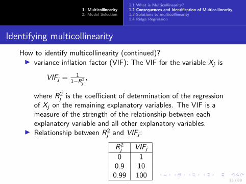
How to identify multicollinearity (continued)?I variance inflation factor (VIF): The VIF for the variable Xj is
VIFj = 11−R2
j,
where R2j is the coefficient of determination of the regression
of Xj on the remaining explanatory variables. The VIF is ameasure of the strength of the relationship between eachexplanatory variable and all other explanatory variables.
I Relationship between R2j and VIFj :
R2j VIFj
0 10.9 10
0.99 100
23 / 89
1. Multicollinearity2. Model Selection
1.1 What is Multicollinearity?1.2 Consequences and Identification of Multicollinearity1.3 Solutions to multicollinearity1.4 Ridge Regression
Identifying multicollinearity
How to identify multicollinearity (continued)?I variance inflation factor (VIF): The VIF for the variable Xj is
VIFj = 11−R2
j,
where R2j is the coefficient of determination of the regression
of Xj on the remaining explanatory variables. The VIF is ameasure of the strength of the relationship between eachexplanatory variable and all other explanatory variables.
I Relationship between R2j and VIFj :
R2j VIFj
0 10.9 10
0.99 10023 / 89

1. Multicollinearity2. Model Selection
1.1 What is Multicollinearity?1.2 Consequences and Identification of Multicollinearity1.3 Solutions to multicollinearity1.4 Ridge Regression
Identifying multicollinearity
I Rule of thumb for using VIF:- An individual VIFj larger than 10 indicates thatmulticollinearity may be seriously influencing the least squaresestimates of regression coefficients.- If the average of the VIFj ’s of the model exceeds 5 thenmuilticollinearity is considered to be serious.- If the VIF are less than 1/(1− R2) then multicollinearity isnot strong enough to affect the coefficient estimates. In thiscase, the independent variables are more strongly related tothe Y variable than they are to each other.
24 / 89

1. Multicollinearity2. Model Selection
1.1 What is Multicollinearity?1.2 Consequences and Identification of Multicollinearity1.3 Solutions to multicollinearity1.4 Ridge Regression
Identifying multicollinearity
I For the HOUSING example,
The REG Procedure Model: MODEL1 Dependent Variable: housing Number of Observations Read 23 Number of Observations Used 23
Analysis of Variance
Sum of Mean Source DF Squares Square F Value Pr > F Model 3 1147699 382566 4.92 0.0108 Error 19 1478302 77805 Corrected Total 22 2626001 Root MSE 278.93613 R-Square 0.4371 Dependent Mean 1601.07826 Adj R-Sq 0.3482 Coeff Var 17.42177 Parameter Estimates Parameter Standard Variance Variable DF Estimate Error t Value Pr > |t| Inflation Intercept 1 -1317.45317 4930.68042 -0.27 0.7922 0 pop 1 14.91398 36.55401 0.41 0.6878 87.97808 gdp 1 0.52186 0.97391 0.54 0.5983 64.66953 intrate 1 -184.77902 58.10610 -3.18 0.0049 7.42535 25 / 89

1. Multicollinearity2. Model Selection
1.1 What is Multicollinearity?1.2 Consequences and Identification of Multicollinearity1.3 Solutions to multicollinearity1.4 Ridge Regression
Solutions to multicollinearity
Solutions to multicollinearity:
I Benign neglect: If an analyst is less interested in interpretingindividual coefficients but more interested in forecasting thenmulticollinearity may not a serious concern. Even with highcorrelations among independent variables, if the regressioncoefficients are significant and have meaningful signs andmagnitudes, one need not be too concerned withmulticollinearity.
26 / 89

1. Multicollinearity2. Model Selection
1.1 What is Multicollinearity?1.2 Consequences and Identification of Multicollinearity1.3 Solutions to multicollinearity1.4 Ridge Regression
Solutions to multicollinearity
I Eliminating Variables: Remove the variable with strongcorrelation with the rest would generally improve thesignificance of other variables. There is a danger, however, inremoving too many variables from the model because thatwould lead to bias in the estimates. Another drawback of thisapproach is that no information is obtained on the omittedvariable.
27 / 89

1. Multicollinearity2. Model Selection
1.1 What is Multicollinearity?1.2 Consequences and Identification of Multicollinearity1.3 Solutions to multicollinearity1.4 Ridge Regression
Solutions to multicollinearity
I Respecify the model: For example, in the housing regression,we can include the variables as per capita rather thanincluding population as an explanatory variable, leading to
HOUSINGi/POPi = β1 + β2GDPi/POPi + β3INTRATEi + εi The REG Procedure
Model: MODEL1 Dependent Variable: phousing Number of Observations Read 23 Number of Observations Used 23 Analysis of Variance Sum of Mean Source DF Squares Square F Value Pr > F Model 2 26.33472 13.16736 7.66 0.0034 Error 20 34.38472 1.71924 Corrected Total 22 60.71944 Root MSE 1.31120 R-Square 0.4337 Dependent Mean 7.50743 Adj R-Sq 0.3771 Coeff Var 17.46531 Parameter Estimates Parameter Standard Variance Variable DF Estimate Error t Value Pr > |t| Inflation Intercept 1 2.07920 3.34724 0.62 0.5415 0 pgdp 1 0.93567 0.36701 2.55 0.0191 3.45825 intrate 1 -0.69832 0.18640 -3.75 0.0013 3.45825
28 / 89

1. Multicollinearity2. Model Selection
1.1 What is Multicollinearity?1.2 Consequences and Identification of Multicollinearity1.3 Solutions to multicollinearity1.4 Ridge Regression
Solutions to multicollinearity
I Increase the sample size if additional information is available.
I Use alternative estimation techniques such as Ridge regressionand principal component analysis. We will touch on Ridgeregression but principal component analysis is beyond thescope of this course.
29 / 89

1. Multicollinearity2. Model Selection
1.1 What is Multicollinearity?1.2 Consequences and Identification of Multicollinearity1.3 Solutions to multicollinearity1.4 Ridge Regression
Ridge Regression
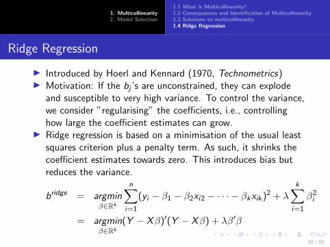
I Introduced by Hoerl and Kennard (1970, Technometrics)I Motivation: If the bj ’s are unconstrained, they can explode
and susceptible to very high variance. To control the variance,we consider ”regularising” the coefficients, i.e., controllinghow large the coefficient estimates can grow.
I Ridge regression is based on a minimisation of the usual leastsquares criterion plus a penalty term. As such, it shrinks thecoefficient estimates towards zero. This introduces bias butreduces the variance.
bridge = argminβ∈Rk
n∑i=1
(yi − β1 − β2xi2 − · · · − βkxik)2 + λk∑
i=1
β2i
= argminβ∈Rk
(Y − Xβ)′(Y − Xβ) + λβ′β
30 / 89
1. Multicollinearity2. Model Selection
1.1 What is Multicollinearity?1.2 Consequences and Identification of Multicollinearity1.3 Solutions to multicollinearity1.4 Ridge Regression
Ridge Regression
I Introduced by Hoerl and Kennard (1970, Technometrics)I Motivation: If the bj ’s are unconstrained, they can explode
and susceptible to very high variance. To control the variance,we consider ”regularising” the coefficients, i.e., controllinghow large the coefficient estimates can grow.
I Ridge regression is based on a minimisation of the usual leastsquares criterion plus a penalty term. As such, it shrinks thecoefficient estimates towards zero. This introduces bias butreduces the variance.
bridge = argminβ∈Rk
n∑i=1
(yi − β1 − β2xi2 − · · · − βkxik)2 + λk∑
i=1
β2i
= argminβ∈Rk
(Y − Xβ)′(Y − Xβ) + λβ′β
30 / 89

1. Multicollinearity2. Model Selection
1.1 What is Multicollinearity?1.2 Consequences and Identification of Multicollinearity1.3 Solutions to multicollinearity1.4 Ridge Regression
Ridge Regression
I This results in the solution
bridge = (X ′X + λI )−1X ′Y
I This is, in general, a biased estimator of β but more efficientthan b:
E (bridge) = (X ′X + λI )−1X ′Xβ
Cov(bridge) = (X ′X + λI )−1X ′X (X ′X + λI )−1
I This bias is zero if λ = 0 but Cov(b)− Cov(bridge) is apositive definite matrix for λ > 0. Over some range of λ,bridge has smaller mean square error (MSE) than b.
31 / 89
1. Multicollinearity2. Model Selection
1.1 What is Multicollinearity?1.2 Consequences and Identification of Multicollinearity1.3 Solutions to multicollinearity1.4 Ridge Regression
Ridge Regression
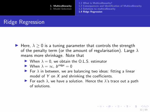
I Here, λ ≥ 0 is a tuning parameter that controls the strengthof the penalty term (or the amount of regularisation). Large λmeans more shrinkage. Note thatI When λ = 0, we obtain the O.L.S. estimatorI When λ =∞, bridge = 0I For λ in between, we are balancing two ideas: fitting a linear
model of Y on X and shrinking the coefficients.I For each λ, we have a solution. Hence the λ’s trace out a path
of solutions.
32 / 89

1. Multicollinearity2. Model Selection
1.1 What is Multicollinearity?1.2 Consequences and Identification of Multicollinearity1.3 Solutions to multicollinearity1.4 Ridge Regression
Ridge Regression
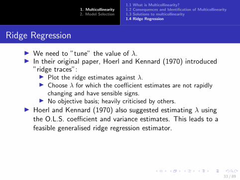
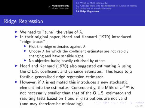
I We need to ”tune” the value of λ.I In their original paper, Hoerl and Kennard (1970) introduced
”ridge traces”:
I Plot the ridge estimates against λ.I Choose λ for which the coefficient estimates are not rapidly
changing and have sensible signs.I No objective basis; heavily criticised by others.
I Hoerl and Kennard (1970) also suggested estimating λ usingthe O.L.S. coefficient and variance estimates. This leads to afeasible generalised ridge regression estimator.
I However, if λ is estimated this introduces a new stochasticelement into the estimator. Consequently, the MSE of bridge isnot necessarily smaller than that of the O.L.S. estimator andresulting tests based on t and F distributions are not valid(and may therefore be misleading).
33 / 89

1. Multicollinearity2. Model Selection
1.1 What is Multicollinearity?1.2 Consequences and Identification of Multicollinearity1.3 Solutions to multicollinearity1.4 Ridge Regression
Ridge Regression
I We need to ”tune” the value of λ.I In their original paper, Hoerl and Kennard (1970) introduced
”ridge traces”:I Plot the ridge estimates against λ.I Choose λ for which the coefficient estimates are not rapidly
changing and have sensible signs.
I No objective basis; heavily criticised by others.I Hoerl and Kennard (1970) also suggested estimating λ using
the O.L.S. coefficient and variance estimates. This leads to afeasible generalised ridge regression estimator.
I However, if λ is estimated this introduces a new stochasticelement into the estimator. Consequently, the MSE of bridge isnot necessarily smaller than that of the O.L.S. estimator andresulting tests based on t and F distributions are not valid(and may therefore be misleading).
33 / 89

1. Multicollinearity2. Model Selection
1.1 What is Multicollinearity?1.2 Consequences and Identification of Multicollinearity1.3 Solutions to multicollinearity1.4 Ridge Regression
Ridge Regression
I We need to ”tune” the value of λ.I In their original paper, Hoerl and Kennard (1970) introduced
”ridge traces”:I Plot the ridge estimates against λ.I Choose λ for which the coefficient estimates are not rapidly
changing and have sensible signs.I No objective basis; heavily criticised by others.
I Hoerl and Kennard (1970) also suggested estimating λ usingthe O.L.S. coefficient and variance estimates. This leads to afeasible generalised ridge regression estimator.
I However, if λ is estimated this introduces a new stochasticelement into the estimator. Consequently, the MSE of bridge isnot necessarily smaller than that of the O.L.S. estimator andresulting tests based on t and F distributions are not valid(and may therefore be misleading).
33 / 89

1. Multicollinearity2. Model Selection
1.1 What is Multicollinearity?1.2 Consequences and Identification of Multicollinearity1.3 Solutions to multicollinearity1.4 Ridge Regression
Ridge Regression
I Example 3.1 The following example comes from a study ofmanpower needs for operating a U.S. Navy Bachelor OfficersQuarters (BOQ). The observations are recorded for 24establishments. The response variable represents the monthlyman-hours (MANH) required to operate each establishment,and the independent variables are:
OCCUP = average daily occupancy
CHECKIN = monthly average number of check-ins
HOURS = weekly hours of service desk operation
COMMON = square feet of common use area
WINGS = number of building wings
CAP = operational berthing capacity
ROOMS = number of rooms 34 / 89

1. Multicollinearity2. Model Selection
1.1 What is Multicollinearity?1.2 Consequences and Identification of Multicollinearity1.3 Solutions to multicollinearity1.4 Ridge Regression
Ridge Regression
I Results obtained using SAS:SAS Output
SAS Output_htm#IDX10.htm[10/31/2016 1:52:19 PM]
The SAS System
The REG ProcedureModel: MODEL1
Dependent Variable: MANH
Number of Observations Read 24
Number of Observations Used 24
Analysis of Variance
Source DFSum of
SquaresMean
Square F Value Pr > F
Model 7 87497673 12499668 154.32 <.0001
Error 16 1295987 80999
Corrected Total 23 88793659
Root MSE 284.60353 R-Square 0.9854
Dependent Mean 2050.00708 Adj R-Sq 0.9790
Coeff Var 13.88305
Parameter Estimates
Variable DFParameter
EstimateStandard
Error t Value Pr > |t|VarianceInflation
Intercept 1 171.47336 148.86168 1.15 0.2663 0
OCCUP 1 21.04562 4.28905 4.91 0.0002 43.63222
CHECKIN 1 1.42632 0.33071 4.31 0.0005 4.54154
HOURS 1 -0.08927 1.16353 -0.08 0.9398 1.36076
COMMON 1 7.65033 8.43835 0.91 0.3781 4.06083
WINGS 1 -5.30231 9.45276 -0.56 0.5826 3.79996
CAP 1 -4.07475 3.30195 -1.23 0.2350 56.60333
ROOMS 1 0.33191 6.81399 0.05 0.9618 178.7015935 / 89

1. Multicollinearity2. Model Selection
1.1 What is Multicollinearity?1.2 Consequences and Identification of Multicollinearity1.3 Solutions to multicollinearity1.4 Ridge Regression
Ridge Regression
I The O.L.S. results clearly indicate serious multicollinearity.I R2 = 0.985 is rather high. Since 1/(1− R2) = 68.5, any
variables associated with VIF values exceeding 68.5 are moreclosely related to other explanatory variables than they are tothe dependent variable.
I ROOMS has a VIF that exceeds 68.5, and it is notstatistically significant.
I OCCUP has a VIF that exceeds 10 and a t − stat with a verysmall p−value. One may conclude that multicollinearity existsthat decreases the reliability of estimates.
I CAP has a large VIF and is not significant; this variable mighthave been useful had it not been associated withmulticollinearity.
36 / 89

1. Multicollinearity2. Model Selection
1.1 What is Multicollinearity?1.2 Consequences and Identification of Multicollinearity1.3 Solutions to multicollinearity1.4 Ridge Regression
Ridge Regression
I The ridge plot is given as follows:The SAS SystemThe SAS System
Coeffici
ent Es
timate
-10
-5
0
5
10
15
20
25
Ridge k
0.0 0.1 0.2 0.3 0.4 0.5 0.6 0.7 0.8 0.9 1.0
Plot OCCUP CHECKIN HOURS COMMONWINGS CAP ROOMS 37 / 89

1. Multicollinearity2. Model Selection
1.1 What is Multicollinearity?1.2 Consequences and Identification of Multicollinearity1.3 Solutions to multicollinearity1.4 Ridge Regression
Ridge Regression
I VIFs of estimates at varying values of λ:SAS Output
SAS Output_htm#IDX10.htm[10/31/2016 3:17:25 PM]
The SAS System
Obs _RIDGE_ OCCUP CHECKIN HOURS COMMON WINGS CAP ROOMS
3 0.00 43.6322 4.54154 1.36076 4.06083 3.79996 56.6033 178.702
6 0.05 3.3779 2.60290 1.16762 1.58426 2.08551 2.8171 1.332
9 0.10 1.5606 1.75533 1.02578 1.27207 1.50400 1.4726 0.539
12 0.15 0.9261 1.28481 0.90939 1.05990 1.17392 0.9523 0.334
15 0.20 0.6270 0.99168 0.81228 0.90266 0.95480 0.6826 0.241
18 0.25 0.4605 0.79480 0.73028 0.78112 0.79775 0.5210 0.189
21 0.30 0.3574 0.65519 0.66033 0.68448 0.67975 0.4152 0.155
24 0.35 0.2886 0.55203 0.60014 0.60600 0.58811 0.3414 0.131
27 0.40 0.2402 0.47330 0.54796 0.54116 0.51516 0.2877 0.114
30 0.45 0.2045 0.41163 0.50240 0.48684 0.45592 0.2470 0.101
33 0.50 0.1774 0.36226 0.46239 0.44078 0.40703 0.2154 0.091
36 0.55 0.1562 0.32203 0.42705 0.40134 0.36612 0.1903 0.083
39 0.60 0.1393 0.28873 0.39567 0.36726 0.33149 0.1700 0.076
42 0.65 0.1255 0.26081 0.36769 0.33757 0.30187 0.1532 0.070
45 0.70 0.1141 0.23713 0.34262 0.31153 0.27632 0.1391 0.066
48 0.75 0.1045 0.21683 0.32007 0.28855 0.25410 0.1273 0.062
51 0.80 0.0963 0.19929 0.29972 0.26815 0.23463 0.1171 0.058
54 0.85 0.0893 0.18400 0.28128 0.24995 0.21748 0.1084 0.055
57 0.90 0.0832 0.17058 0.26452 0.23363 0.20227 0.1007 0.052
60 0.95 0.0779 0.15873 0.24924 0.21895 0.18871 0.0941 0.050 38 / 89

1. Multicollinearity2. Model Selection
1.1 What is Multicollinearity?1.2 Consequences and Identification of Multicollinearity1.3 Solutions to multicollinearity1.4 Ridge Regression
Ridge Regression
I Coefficient estimates at varying values of λ:SAS Output
SAS Output_htm#IDX10.htm[10/31/2016 3:17:25 PM]
The SAS System
Obs _RIDGE_ Intercept OCCUP CHECKIN HOURS COMMON WINGS CAP ROOMS
4 0.00 171.473 21.0456 1.42632 -0.08927 7.65033 -5.3023 -4.07475 0.33191
7 0.05 150.557 12.2806 1.53469 0.38682 0.51146 9.7589 -1.47494 2.86432
10 0.10 140.775 9.7164 1.49356 0.62657 -0.24718 14.0025 -0.16568 2.95724
13 0.15 135.946 8.3991 1.43806 0.79962 -0.05448 15.7514 0.51504 2.99289
16 0.20 134.517 7.5788 1.38536 0.93650 0.41616 16.6172 0.92646 3.00585
19 0.25 135.604 7.0087 1.33797 1.04940 0.96391 17.0913 1.19731 3.00591
22 0.30 138.627 6.5829 1.29571 1.14469 1.51548 17.3648 1.38550 2.99787
25 0.35 143.178 6.2487 1.25789 1.22625 2.04212 17.5248 1.52105 2.98452
28 0.40 148.955 5.9765 1.22380 1.29674 2.53300 17.6152 1.62115 2.96763
31 0.45 155.725 5.7485 1.19285 1.35805 2.98510 17.6603 1.69630 2.94833
34 0.50 163.307 5.5532 1.16456 1.41164 3.39890 17.6742 1.75333 2.92739
37 0.55 171.555 5.3830 1.13852 1.45864 3.77643 17.6658 1.79684 2.90537
40 0.60 180.350 5.2325 1.11444 1.49997 4.12031 17.6408 1.83003 2.88264
43 0.65 189.594 5.0978 1.09203 1.53637 4.43336 17.6033 1.85522 2.85947
46 0.70 199.208 4.9760 1.07111 1.56847 4.71830 17.5558 1.87409 2.83607
49 0.75 209.124 4.8649 1.05147 1.59677 4.97770 17.5006 1.88792 2.81258
52 0.80 219.284 4.7629 1.03299 1.62173 5.21392 17.4389 1.89769 2.78911
55 0.85 229.641 4.6686 1.01554 1.64371 5.42912 17.3722 1.90415 2.76573
58 0.90 240.155 4.5809 0.99901 1.66305 5.62523 17.3011 1.90789 2.74252
61 0.95 250.789 4.4990 0.98330 1.68002 5.80401 17.2266 1.90939 2.71951 39 / 89

1. Multicollinearity2. Model Selection
1.1 What is Multicollinearity?1.2 Consequences and Identification of Multicollinearity1.3 Solutions to multicollinearity1.4 Ridge Regression
Ridge Regression
I Picking a value of λ is quite subjective. It appears that thecoefficient estimates stabilise at around λ = 0.65. The VIF’sare also reasonably small at λ = 0.65 and the coefficientestimates have the right signs.
SAS Output
SAS Output_htm#IDX10.htm[10/31/2016 3:17:25 PM]
The SAS System
Obs _TYPE_ Intercept OCCUP CHECKIN HOURS COMMON WINGS CAP ROOMS
1 PARMS 171.473 21.0456 1.42632 -0.08927 7.65033 -5.3023 -4.07475 0.33191
2 SEB 148.862 4.2890 0.33071 1.16353 8.43835 9.4528 3.30195 6.81399
3 RIDGEVIF . 0.1255 0.26081 0.36769 0.33757 0.3019 0.15317 0.07038
4 RIDGE 189.594 5.0978 1.09203 1.53637 4.43336 17.6033 1.85522 2.85947
5 RIDGESEB 243.906 0.5262 0.18130 1.38363 5.56579 6.0951 0.39295 0.30936
40 / 89

1. Multicollinearity2. Model Selection
1.1 What is Multicollinearity?1.2 Consequences and Identification of Multicollinearity1.3 Solutions to multicollinearity1.4 Ridge Regression
Ridge Regression
DATA BOQ; INPUT id $ OCCUP CHECKIN HOURS COMMON WINGS CAP ROOMS MANH; DROP ID; CARDS; A 2 4 4 1.26 1 6 6 180.23 B 3 1.58 40 1.25 1 5 5 182.61 C 16.6 23.78 40 1 1 13 13 164.38 : : X 384.5 1473.66 168 7.36 24 540 453 8266.77 Y 95 368 168 30.26 9 292 196 1845.89 ; proc reg data=boq; model manh=occup checkin hours common wings cap rooms/vif; run; proc reg data=boq outvif outseb outest=bfout ridge=0 to 1.0 by 0.02; model manh=occup checkin hours common wings cap rooms/noprint; plot/ridgeplot nomodel nostat; run; proc print data =bfout; var _RIDGE_ occup checkin hours common wings cap rooms; where _TYPE_='RIDGEVIF'; run; proc print data=bfout; var _RIDGE_ intercept occup checkin hours common wings cap rooms; where _TYPE_='RIDGE'; run;
41 / 89
1. Multicollinearity2. Model Selection
2.1 Model Selection Techniques2.2 Mallows’ Cp2.3 Akaike’s Information Criterion and Related Measures2.4 Least Absolute Shrinkage and Selection Operator2.5 Model Averaging
Model Selection Techniques
I We consider two broad types of model selection techniques:all possible regressions and penalised regression.
I Penalised regression bears a similarity to Ridge regressionexcept that penalised regression actually allows somecoefficients to become identically zero.
I For all possible regressions, we consider the followingcommonly used criteria for choosing between models:I Adjusted R2 Criterion - select the model with the highest
adjusted R2
I Mallows’ Cp CriterionI Information Criterion
42 / 89

1. Multicollinearity2. Model Selection
2.1 Model Selection Techniques2.2 Mallows’ Cp2.3 Akaike’s Information Criterion and Related Measures2.4 Least Absolute Shrinkage and Selection Operator2.5 Model Averaging
Model Selection Techniques
I In the process we will also examine the effects of omittingimportant regressors and including irrelevant regressors.
I If important variables are omitted the effects of these variablesare not taken into account. The estimators of othercoefficients will become biased.
I If unimportant variables are included then the variances ofcoefficient estimators will become inflated. Thus, forecastsand estimates will become more variable than they would behad the irrelevant regressors been excluded.
43 / 89

1. Multicollinearity2. Model Selection
2.1 Model Selection Techniques2.2 Mallows’ Cp2.3 Akaike’s Information Criterion and Related Measures2.4 Least Absolute Shrinkage and Selection Operator2.5 Model Averaging
Mallows’ Cp
I The Mallows’ Cp is one of the most commonly used criteriafor choosing between alternative regressions with differentcombinations of regressors. The Cp’s formula is given by
Cp =SSEp
MSEF− (n − 2p)
where SSEp is the sum of squared errors of the regression withp coefficients and MSEF is the MSE corresponding to the fullmodel, the model that contains all of the explanatoryvariables.
44 / 89

1. Multicollinearity2. Model Selection
2.1 Model Selection Techniques2.2 Mallows’ Cp2.3 Akaike’s Information Criterion and Related Measures2.4 Least Absolute Shrinkage and Selection Operator2.5 Model Averaging
Mallows’ Cp
I When the estimated regression has no bias, Cp is equal to p.When evaluating which model is best, it is recommended thatregression with small Cp values and those with values close top be considered. If Cp is substantially larger than p, thenthere is a large bias component in the model.
45 / 89

1. Multicollinearity2. Model Selection
2.1 Model Selection Techniques2.2 Mallows’ Cp2.3 Akaike’s Information Criterion and Related Measures2.4 Least Absolute Shrinkage and Selection Operator2.5 Model Averaging
Mallows’ Cp
I The development of the Mallows’ Cp is based on theestimation of the trace of the MSE (also known as risk undersquared error loss) of an estimator of Xβ scaled by σ2.
I Consider the O.L.S. predictor Xb, the risk of Xb is given byR(Xb)
=E [(Xb − Xβ)′(Xb − Xβ)]
=E [(Xb − E (Xb) + E (Xb)− Xβ)′(Xb − E (Xb) + E (Xb)− Xβ)]
=E [(Xb − E (Xb))′(Xb − E (Xb))] + (E (Xb)− Xβ)′(E (Xb)− Xβ)
46 / 89

1. Multicollinearity2. Model Selection
2.1 Model Selection Techniques2.2 Mallows’ Cp2.3 Akaike’s Information Criterion and Related Measures2.4 Least Absolute Shrinkage and Selection Operator2.5 Model Averaging
Mallows’ Cp
I The first term is the sum of the variances of the elements ofY = Xb, while the second term is the sum of the bias squaresof the elements of Y when E (Y ) = Xβ is the unknownquantity of interest.
I Assuming that the model is correctly specified such thatE (ε) = 0, b is unbiased and the second term vanishes to zero.
I If b is unbiased, the first term (the sum of variances) may bewritten as
E (ε′X (X ′X )−1X ′ε)
=E [tr((X ′X )−1X ′εε′X )]
=σ2k
47 / 89

1. Multicollinearity2. Model Selection
2.1 Model Selection Techniques2.2 Mallows’ Cp2.3 Akaike’s Information Criterion and Related Measures2.4 Least Absolute Shrinkage and Selection Operator2.5 Model Averaging
Mallows’ Cp
I Now, suppose that the choice of X is uncertain and Xp isused as the regressor matrix instead. So,
Y = Xpβp + u
where u = ε+ Xeβe or u = ε− Xeβe .
I Thus, bp = (X ′pXp)−1X ′pY and
Xpbp − E (Xpbp) = Xp(βp + (X ′pXp)−1X ′pε± (X ′pXp)−1X ′pXeβe)
−Xpβp ∓ (X ′pXp)−1X ′pXeβe
= Xp(X ′pXp)−1X ′pε
I Hence
E [(Xpbp − E (Xpbp))′(Xpbp − E (Xpbp))] = σ2p
48 / 89

1. Multicollinearity2. Model Selection
2.1 Model Selection Techniques2.2 Mallows’ Cp2.3 Akaike’s Information Criterion and Related Measures2.4 Least Absolute Shrinkage and Selection Operator2.5 Model Averaging
Mallows’ Cp
I Now, suppose that the choice of X is uncertain and Xp isused as the regressor matrix instead. So,
Y = Xpβp + u
where u = ε+ Xeβe or u = ε− Xeβe .I Thus, bp = (X ′pXp)−1X ′pY and
Xpbp − E (Xpbp) = Xp(βp + (X ′pXp)−1X ′pε± (X ′pXp)−1X ′pXeβe)
−Xpβp ∓ (X ′pXp)−1X ′pXeβe
= Xp(X ′pXp)−1X ′pε
I Hence
E [(Xpbp − E (Xpbp))′(Xpbp − E (Xpbp))] = σ2p48 / 89

1. Multicollinearity2. Model Selection
2.1 Model Selection Techniques2.2 Mallows’ Cp2.3 Akaike’s Information Criterion and Related Measures2.4 Least Absolute Shrinkage and Selection Operator2.5 Model Averaging
Mallows’ Cp
I So, the sum of the variances of y1, · · · , yn changes from σ2kto σ2p as the number of coefficients changes from k to p.Thus, if the model is under-fitted (i.e., p < k), the sum of thevariances actually decreases whereas if the model is over-fitted(i.e., p > k), this sum increases.
I However, when the model is misspecified, the second term inthe MSE expression related to the bias is not always zero.Note that
E (Xpbp) = Xp(X ′pXp)−1X ′pXβ,
which equals Xβ if Xpbp is unbiased.
49 / 89

1. Multicollinearity2. Model Selection
2.1 Model Selection Techniques2.2 Mallows’ Cp2.3 Akaike’s Information Criterion and Related Measures2.4 Least Absolute Shrinkage and Selection Operator2.5 Model Averaging
Mallows’ Cp
I Obviously, when the model is under-fitted,Xp(X ′pXp)−1X ′pXβ 6= Xβ. That is, a bias is introduced to theestimator of E (Y ).
I On the other hand, when the model is over-fitted, we canwrite X = XpZ , where
Z =
[I(k×k)
0((p−k)×k)
]leading to Xp(X ′pXp)−1X ′pXβ = Xβ. That is, the estimatorremains unbiased when the model is over-fitted.
50 / 89

1. Multicollinearity2. Model Selection
2.1 Model Selection Techniques2.2 Mallows’ Cp2.3 Akaike’s Information Criterion and Related Measures2.4 Least Absolute Shrinkage and Selection Operator2.5 Model Averaging
Mallows’ Cp
I So, when the model is under-fitted, the O.L.S. estimator ofE (Y ) is biased but has a reduced sum of variances. When themodel is over-fitted, the O.L.S. estimator of E (Y ) remainsunbiased but its sum of variances increases.
I Now, the sum of bias squares of Y is
(E (Xpbp)− Xβ)′(E (Xpbp)− Xβ)
= (Xp(X ′pXp)−1X ′pXβ − Xβ)′(Xp(X ′pXp)−1X ′pXβ − Xβ)
= β′X ′(I − Xp(X ′pXp)−1X ′p)Xβ
51 / 89

1. Multicollinearity2. Model Selection
2.1 Model Selection Techniques2.2 Mallows’ Cp2.3 Akaike’s Information Criterion and Related Measures2.4 Least Absolute Shrinkage and Selection Operator2.5 Model Averaging
Mallows’ Cp
I To estimate the bias which is unobservable, note that
(Y − Xpbp)′(Y − Xpbp) = Y ′(I − Xp(X ′pXp)−1X ′p)Y = SSEp
is the sum of squared errors in the observation sample basedon the estimated model with p coefficients. Using Theorem1.17 of Seber (2008): A Matrix Handbook for Statisticians,E (Y ′AY ) = E (Y ′)AE (Y ) + tr(ΣA), where Σ is the Cov(Y ),we can write
E ((Y − Xpbp)′(Y − Xpbp))
= E (Y ′)(I − Xp(X ′pXp)−1X ′p)E (Y ) + tr(I − Xp(X ′pXp)−1X ′p)σ2
= β′X ′(I − Xp(X ′pXp)−1X ′p)Xβ + σ2n − σ2p
52 / 89

1. Multicollinearity2. Model Selection
2.1 Model Selection Techniques2.2 Mallows’ Cp2.3 Akaike’s Information Criterion and Related Measures2.4 Least Absolute Shrinkage and Selection Operator2.5 Model Averaging
Mallows’ Cp
I The first term is the sum of the bias squares. We canestimate this sum by SSEp − σ2(n − p).
I Recall that the Mallows’ Cp is defined as R(Xpbp)/σ2. By ourderivation,
R(Xpbp)/σ2 = p +SSEp − σ2(n − p)
σ2
I σ2 is unknown but can be estimated by e ′e/(n − k), the MSEin the ANOVA table of the full model. This yields the formula:
Cp = p +SSEp
MSEF− n + p
=SSEp
MSEF− (n − 2p)
53 / 89

1. Multicollinearity2. Model Selection
2.1 Model Selection Techniques2.2 Mallows’ Cp2.3 Akaike’s Information Criterion and Related Measures2.4 Least Absolute Shrinkage and Selection Operator2.5 Model Averaging
Mallows’ Cp
I Thus, if the model is correctly specified, the bias is zero andthe (scaled) sum of variances (and hence the Cp) should equalp.
I For two models with Cp’s that are both close to theirrespective p’s, the model with the smaller Cp is preferred tothe model with the larger Cp because a large Cp probablyindicates over-fitting which results in a larger sum of variancesthan otherwise.
I When the model is grossly under-fitted, the bias term willdominate the reduced variance, leading to a value of Cp
substantially larger than p.
54 / 89

1. Multicollinearity2. Model Selection
2.1 Model Selection Techniques2.2 Mallows’ Cp2.3 Akaike’s Information Criterion and Related Measures2.4 Least Absolute Shrinkage and Selection Operator2.5 Model Averaging
Information Criteria
I Information Criteria use the observed data to give a candidatemodel a certain score; this then leads to a fully ranked list ofcandidate models from worst to best.
I Virtually all Information Criteria are penalised version of theattained maximum log-likelihood of the model, aimed atbalancing between goodness of fit (high value oflog-likelihood) and complexity (complex models are penalisedmore than simple ones).
55 / 89
1. Multicollinearity2. Model Selection
2.1 Model Selection Techniques2.2 Mallows’ Cp2.3 Akaike’s Information Criterion and Related Measures2.4 Least Absolute Shrinkage and Selection Operator2.5 Model Averaging
Likelihood Function and Maximum Likelihood
I Suppose that a sample of observations (y1, y2, · · · , yn) isavailable, and it is assumed that each yi is drawn from someparticular distribution which has a probability density functionp(yi |β). Assuming that the yi ’s are independent, the jointdensity of the sample is given by
p(y1|β)p(y2|β) · · · p(yn|β) =n∏
i=1
p(yi |β) = f (y |β) = L(β|y)
56 / 89

1. Multicollinearity2. Model Selection
2.1 Model Selection Techniques2.2 Mallows’ Cp2.3 Akaike’s Information Criterion and Related Measures2.4 Least Absolute Shrinkage and Selection Operator2.5 Model Averaging
Likelihood Function and Maximum Likelihood
I L(β|y) is the likelihood function which is a function of theparameters for a given set of observations.
I Clearly, the value of L(β|y) will be higher for some values of βthan for others, and the method of maximum likelihoodanswers the question:What value of the parameters maximises the likelihood?
I Denote this parameter value by bMLE . The joint densityf (y |β) is then maximised at bMLE , and so bMLE is theparameter value that maximises the probability of observingthe sample at hand.
57 / 89
1. Multicollinearity2. Model Selection
2.1 Model Selection Techniques2.2 Mallows’ Cp2.3 Akaike’s Information Criterion and Related Measures2.4 Least Absolute Shrinkage and Selection Operator2.5 Model Averaging
Likelihood Function and Maximum Likelihood
I In practice, maximum likelihood typically does not use thelikelihood function itself, but uses the log-likelihood function
lnL(β|y) = lnf (y |β) =n∑
i=1
lnp(yi |β)
I The advantage of working with the log-likelihood is that thisis an additive rather than a multiplicative function andmaximising this function is analytically easier than maximisingthe likelihood itself. Of course the two approaches lead to thesame solution because the log-likelihood is a monotonictransformation of the likelihood.
58 / 89

1. Multicollinearity2. Model Selection
2.1 Model Selection Techniques2.2 Mallows’ Cp2.3 Akaike’s Information Criterion and Related Measures2.4 Least Absolute Shrinkage and Selection Operator2.5 Model Averaging
Akaike’s Information Criterion
I The Akaike’s Information Criterion (AIC) is arguably the mostpopular information criteria due to its ease. For the sth
model, the AIC is defined as
AICs = −2lnf (y |bs) + 2ks
where lnf (y |bs) and ks are the (computed) log-likelihood ofand the number of coefficients in the sth model respectively.
I lnf (y |bs) is the goodness of fit term and ks is the penaltyterm.
59 / 89

1. Multicollinearity2. Model Selection
2.1 Model Selection Techniques2.2 Mallows’ Cp2.3 Akaike’s Information Criterion and Related Measures2.4 Least Absolute Shrinkage and Selection Operator2.5 Model Averaging
Akaike’s Information Criterion
I To develop the AIC, let g(y) be the true (and unknown) p.d.f.of Y . To assess the similarity between g(y) and f (y |βs), weconsider the Kullback-Leibler Information:
I (βs) = E [lng(y)
f (y |βs)]
where E (.) is taken w.r.t. g(y), the true density.
I It can be shown that I (βs) ≥ 0 with equality ifff (y |βs) = g(y). As the disparity between f (y |βs) and g(y)grows, I (βs) increases to reflect this disparity.
60 / 89

1. Multicollinearity2. Model Selection
2.1 Model Selection Techniques2.2 Mallows’ Cp2.3 Akaike’s Information Criterion and Related Measures2.4 Least Absolute Shrinkage and Selection Operator2.5 Model Averaging
Akaike’s Information Criterion
I Write
2I (βs) = 2E [lng(y)− lnf (y |βs)]
= −E [−2lng(y)] + E [−2lnf (y |βs)]
= −E [−2lng(y)] + d(βs)
where d(βs) is the Kullback discrepancy. As E[−2lng(y)] doesnot depend on βs , any ranking of models based onKullback-Leibler Information is equivalent to ranking based onthe Kullback discrepancy.
61 / 89

1. Multicollinearity2. Model Selection
2.1 Model Selection Techniques2.2 Mallows’ Cp2.3 Akaike’s Information Criterion and Related Measures2.4 Least Absolute Shrinkage and Selection Operator2.5 Model Averaging
Akaike’s Information Criterion
I To evaluate the separation between the fitted candidate modeland the true model, we consider the Kullback discrepancyevaluated at
d(bs) = E [−2lnf (y |βs)]|βs=bs
I But d(bs) cannot be computed. Why?I Akaike (1973) showed that −2lnf (y |bs) is a biased estimator
of d(bs) and the bias adjustment
E [−2lnf (y |βs)]|βs=bs − E [−2lnf (y |bs)]
can be approximated by 2 times the dimension of bs (undersome very strong assumptions).
62 / 89
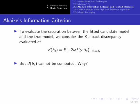
1. Multicollinearity2. Model Selection
2.1 Model Selection Techniques2.2 Mallows’ Cp2.3 Akaike’s Information Criterion and Related Measures2.4 Least Absolute Shrinkage and Selection Operator2.5 Model Averaging
Akaike’s Information Criterion
I To evaluate the separation between the fitted candidate modeland the true model, we consider the Kullback discrepancyevaluated at
d(bs) = E [−2lnf (y |βs)]|βs=bs
I But d(bs) cannot be computed. Why?
I Akaike (1973) showed that −2lnf (y |bs) is a biased estimatorof d(bs) and the bias adjustment
E [−2lnf (y |βs)]|βs=bs − E [−2lnf (y |bs)]
can be approximated by 2 times the dimension of bs (undersome very strong assumptions).
62 / 89

1. Multicollinearity2. Model Selection
2.1 Model Selection Techniques2.2 Mallows’ Cp2.3 Akaike’s Information Criterion and Related Measures2.4 Least Absolute Shrinkage and Selection Operator2.5 Model Averaging
Akaike’s Information Criterion
I To evaluate the separation between the fitted candidate modeland the true model, we consider the Kullback discrepancyevaluated at
d(bs) = E [−2lnf (y |βs)]|βs=bs
I But d(bs) cannot be computed. Why?I Akaike (1973) showed that −2lnf (y |bs) is a biased estimator
of d(bs) and the bias adjustment
E [−2lnf (y |βs)]|βs=bs − E [−2lnf (y |bs)]
can be approximated by 2 times the dimension of bs (undersome very strong assumptions).
62 / 89

1. Multicollinearity2. Model Selection
2.1 Model Selection Techniques2.2 Mallows’ Cp2.3 Akaike’s Information Criterion and Related Measures2.4 Least Absolute Shrinkage and Selection Operator2.5 Model Averaging
Akaike’s Information Criterion
I This leads to the AIC
AICs = −2lnf (y |bs) + 2ks
I A model that is too simplistic will be characterised by arelatively small f (y |bs) (or equivalently, a relatively large−2f (y |bs). On the other hand, a model that conforms to thedata but at the expense of a large number of coefficients willbe characterised by a large f (y |bs) but also large penalty term.
I Models that provide a good balance between the fidelity to thedata and parsimony should correspond to small AIC values.
63 / 89
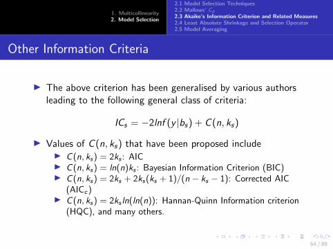
1. Multicollinearity2. Model Selection
2.1 Model Selection Techniques2.2 Mallows’ Cp2.3 Akaike’s Information Criterion and Related Measures2.4 Least Absolute Shrinkage and Selection Operator2.5 Model Averaging
Other Information Criteria
I The above criterion has been generalised by various authorsleading to the following general class of criteria:
ICs = −2lnf (y |bs) + C (n, ks)
I Values of C (n, ks) that have been proposed includeI C (n, ks) = 2ks : AICI C (n, ks) = ln(n)ks : Bayesian Information Criterion (BIC)I C (n, ks) = 2ks + 2ks(ks + 1)/(n − ks − 1): Corrected AIC
(AICc)I C (n, ks) = 2ks ln(ln(n)): Hannan-Quinn Information criterion
(HQC), and many others.
64 / 89

1. Multicollinearity2. Model Selection
2.1 Model Selection Techniques2.2 Mallows’ Cp2.3 Akaike’s Information Criterion and Related Measures2.4 Least Absolute Shrinkage and Selection Operator2.5 Model Averaging
Other Information Criteria
I The AIC and BIC are by far the best known. Despite theirsimilarity in terms of formulae, the AIC and BIC are derivedbased on very different assumptions. To derive the BIC, onehas to put a prior probability that model s is the true model.In the derivation, the terms involving the prior are of lowerorders than the terms that appear in the formula for the BICso they have been dropped. The derivation of BIC requiressome knowledge of Bayesian Statistics and is beyond thescope of this course.
I The BIC behaves quite differently from the AIC. It is alsobased on different assumptions. BIC assumes that one of themodels is true and one tries to find the model most likely tobe true in the Bayesian sense. AIC tries to find the model thatpredicts the best.
65 / 89

1. Multicollinearity2. Model Selection
2.1 Model Selection Techniques2.2 Mallows’ Cp2.3 Akaike’s Information Criterion and Related Measures2.4 Least Absolute Shrinkage and Selection Operator2.5 Model Averaging
Other Information Criteria
I The BIC tends to choose simpler models and the penaltyimposed on large models is higher for BIC than for AIC.
I In settings where n is small and ks is comparatively large, 2ksis often much smaller than the bias adjustment, making AICsubstantially biased.
I When the candidate class consists of the normal linearregression models, under the assumption that g(y) belongs inthe candidate class, the bias adjustment term can be exactlyevaluated, leading to the AICc criterion.
66 / 89

1. Multicollinearity2. Model Selection
2.1 Model Selection Techniques2.2 Mallows’ Cp2.3 Akaike’s Information Criterion and Related Measures2.4 Least Absolute Shrinkage and Selection Operator2.5 Model Averaging
Equivalence between AIC and Cp
I If one assumes Y ∼ N(Xβ, σ2) and σ2 is known then AICs
and Cp are equivalent.
I Note that under the above assumption,
AICs = −2lnf (y |bs) + 2ks
= −2[−n
2ln2πσ2 − (Y − Xbs)′(Y − Xbs)/(2σ2)] + 2ks
I If one replaces σ2 by MSEF , thenAICs=constant+ SSEs
MSEF+ 2ks=Cp+n+constant
67 / 89

1. Multicollinearity2. Model Selection
2.1 Model Selection Techniques2.2 Mallows’ Cp2.3 Akaike’s Information Criterion and Related Measures2.4 Least Absolute Shrinkage and Selection Operator2.5 Model Averaging
Model Selection Example The RSQUARE Procedure Model: MODEL1 Dependent Variable: MANH R-Square Selection Method Number in Adjusted Model R-Square R-Square C(p) AIC BIC Variables in Model 1 0.8895 0.8847 27.4820 326.5911 326.1846 ROOMS 1 0.8179 0.8099 58.9192 339.0868 337.3936 CHECKIN 1 0.7968 0.7880 68.1609 341.8224 339.9083 CAP 1 0.5409 0.5209 180.4582 362.2009 359.1629 WINGS 1 0.4101 0.3844 237.8524 368.4678 365.2218 OCCUP 1 0.3268 0.2975 274.3945 371.7691 368.4319 COMMON 1 0.2405 0.2075 312.2770 374.7857 371.3745 HOURS -------------------------------------------------------------------------------------------------- 2 0.9226 0.9155 14.9768 319.7033 319.9785 CHECKIN ROOMS 2 0.9103 0.9021 20.3718 323.3876 322.9310 CAP ROOMS 2 0.8979 0.8886 25.7924 326.6123 325.5706 CHECKIN WINGS 2 0.8944 0.8848 27.3227 327.4522 326.2666 COMMON ROOMS 2 0.8906 0.8806 29.0229 328.3533 327.0171 HOURS ROOMS 2 0.8904 0.8805 29.0818 328.3839 327.0427 WINGS ROOMS 2 0.8895 0.8795 29.4768 328.5885 327.2137 OCCUP ROOMS 2 0.8734 0.8619 36.5354 331.9869 330.0832 CHECKIN CAP 2 0.8445 0.8304 49.2378 337.1363 334.5315 CHECKIN COMMON 2 0.8288 0.8132 56.1254 339.5403 336.6466 WINGS CAP 2 0.8284 0.8128 56.3169 339.6040 336.7029 OCCUP CHECKIN 2 0.8231 0.8071 58.6026 340.3514 337.3654 CHECKIN HOURS 2 0.8091 0.7917 64.7768 342.2653 339.0713 OCCUP CAP 2 0.8028 0.7849 67.5195 343.0706 339.7931 HOURS CAP 2 0.7995 0.7813 68.9882 343.4914 340.1712 COMMON CAP 2 0.6447 0.6124 136.8918 357.7904 353.3426 OCCUP WINGS 2 0.5926 0.5556 159.7532 361.2115 356.5710 HOURS WINGS 2 0.5494 0.5084 178.7301 363.7339 358.9663 COMMON WINGS 2 0.5333 0.4908 185.7981 364.6120 359.8029 OCCUP COMMON 2 0.4918 0.4456 204.0178 366.7426 361.8385 OCCUP HOURS 2 0.4116 0.3582 239.1687 370.4017 365.3513 HOURS COMMON -------------------------------------------------------------------------------------------------- 3 0.9474 0.9398 6.0961 312.0529 314.6988 CHECKIN CAP ROOMS 3 0.9306 0.9207 13.4419 318.9568 319.4628 CHECKIN WINGS ROOMS 3 0.9265 0.9161 15.2299 320.3837 320.4885 COMMON CAP ROOMS 3 0.9232 0.9122 16.7034 321.5013 321.3021 CHECKIN COMMON ROOMS 3 0.9228 0.9118 16.8831 321.6343 321.3994 OCCUP CHECKIN ROOMS 3 0.9227 0.9117 16.9124 321.6559 321.4153 CHECKIN HOURS ROOMS 3 0.9124 0.8999 21.4414 324.7897 323.7479 WINGS CAP ROOMS 3 0.9116 0.8990 21.7683 325.0014 323.9080 OCCUP CAP ROOMS 3 0.9114 0.8988 21.8649 325.0637 323.9552 CHECKIN WINGS CAP 3 0.9110 0.8983 22.0492 325.1819 324.0448 HOURS CAP ROOMS 3 0.8995 0.8852 27.0838 328.2137 326.3757 OCCUP CHECKIN WINGS 3 0.8986 0.8842 27.4798 328.4372 326.5500 CHECKIN HOURS WINGS 3 0.8982 0.8836 27.6839 328.5517 326.6395 COMMON WINGS ROOMS 3 0.8979 0.8833 27.7922 328.6122 326.6868 CHECKIN COMMON WINGS
68 / 89

1. Multicollinearity2. Model Selection
2.1 Model Selection Techniques2.2 Mallows’ Cp2.3 Akaike’s Information Criterion and Related Measures2.4 Least Absolute Shrinkage and Selection Operator2.5 Model Averaging
Model Selection Example The RSQUARE Procedure Model: MODEL1 Dependent Variable: MANH R-Square Selection Method Number in Adjusted Model R-Square R-Square C(p) AIC BIC Variables in Model 3 0.8960 0.8811 28.6417 329.0819 327.0548 HOURS COMMON ROOMS 3 0.8945 0.8794 29.3148 329.4479 327.3426 OCCUP COMMON ROOMS 3 0.8914 0.8759 30.6358 330.1510 327.8979 HOURS WINGS ROOMS 3 0.8906 0.8749 31.0199 330.3517 328.0571 OCCUP HOURS ROOMS 3 0.8904 0.8748 31.0708 330.3782 328.0781 OCCUP WINGS ROOMS 3 0.8787 0.8613 36.2417 332.9324 330.1261 CHECKIN COMMON CAP 3 0.8760 0.8582 37.4289 333.4837 330.5736 OCCUP CHECKIN CAP 3 0.8748 0.8569 37.9520 333.7229 330.7682 CHECKIN HOURS CAP 3 0.8510 0.8298 48.3663 338.0615 334.3585 OCCUP CHECKIN COMMON 3 0.8460 0.8240 50.5756 338.8925 335.0583 CHECKIN HOURS COMMON 3 0.8369 0.8136 54.5670 340.3272 336.2750 OCCUP WINGS CAP 3 0.8325 0.8086 56.4817 340.9873 336.8384 OCCUP CHECKIN HOURS 3 0.8325 0.8086 56.4905 340.9903 336.8410 HOURS WINGS CAP 3 0.8303 0.8061 57.4600 341.3179 337.1215 COMMON WINGS CAP 3 0.8139 0.7873 64.6803 343.6317 339.1172 OCCUP HOURS CAP 3 0.8114 0.7845 65.7512 343.9573 339.4001 OCCUP COMMON CAP 3 0.8045 0.7765 68.8034 344.8628 340.1894 HOURS COMMON CAP 3 0.6724 0.6256 126.7416 357.7618 351.7884 OCCUP HOURS WINGS 3 0.6491 0.5989 136.9902 359.4836 353.3790 OCCUP COMMON WINGS 3 0.5951 0.5373 160.6508 363.0568 356.7059 HOURS COMMON WINGS 3 0.5698 0.5084 171.7602 364.5733 358.1275 OCCUP HOURS COMMON -------------------------------------------------------------------------------------------------- 4 0.9543 0.9451 5.0652 310.5360 314.8744 CHECKIN COMMON CAP ROOMS 4 0.9511 0.9413 6.4497 312.2041 315.8045 OCCUP CHECKIN CAP ROOMS 4 0.9476 0.9371 8.0071 313.9564 316.8076 CHECKIN WINGS CAP ROOMS 4 0.9474 0.9369 8.0848 314.0408 316.8566 CHECKIN HOURS CAP ROOMS 4 0.9339 0.9207 14.0038 319.7471 320.3285 CHECKIN COMMON WINGS ROOMS 4 0.9311 0.9173 15.2365 320.7876 320.9958 OCCUP COMMON CAP ROOMS 4 0.9308 0.9169 15.3728 320.9001 321.0685 OCCUP CHECKIN WINGS ROOMS 4 0.9307 0.9168 15.4177 320.9370 321.0924 CHECKIN HOURS WINGS ROOMS 4 0.9281 0.9137 16.5667 321.8639 321.6971 HOURS COMMON CAP ROOMS 4 0.9267 0.9121 17.1430 322.3162 321.9952 COMMON WINGS CAP ROOMS 4 0.9235 0.9082 18.5787 323.4087 322.7233 OCCUP CHECKIN COMMON ROOMS 4 0.9234 0.9081 18.5978 323.4228 322.7328 CHECKIN HOURS COMMON ROOMS 4 0.9229 0.9075 18.8166 323.5851 322.8420 OCCUP CHECKIN HOURS ROOMS 4 0.9147 0.8977 22.4140 326.1125 324.5743 OCCUP WINGS CAP ROOMS 4 0.9131 0.8957 23.1214 326.5807 324.9018 HOURS WINGS CAP ROOMS 4 0.9124 0.8949 23.4318 326.7835 325.0442 OCCUP HOURS CAP ROOMS 4 0.9120 0.8944 23.6129 326.9010 325.1269 OCCUP CHECKIN WINGS CAP 4 0.9120 0.8944 23.6175 326.9040 325.1291 CHECKIN COMMON WINGS CAP 4 0.9117 0.8940 23.7484 326.9886 325.1887 CHECKIN HOURS WINGS CAP 4 0.9002 0.8802 28.8117 330.0589 327.3964 OCCUP CHECKIN HOURS WINGS 4 0.8998 0.8798 28.9529 330.1393 327.4554 HOURS COMMON WINGS ROOMS 4 0.8995 0.8794 29.0834 330.2135 327.5097 OCCUP CHECKIN COMMON WINGS
69 / 89

1. Multicollinearity2. Model Selection
2.1 Model Selection Techniques2.2 Mallows’ Cp2.3 Akaike’s Information Criterion and Related Measures2.4 Least Absolute Shrinkage and Selection Operator2.5 Model Averaging
Model Selection Example The RSQUARE Procedure Model: MODEL1 Dependent Variable: MANH R-Square Selection Method Number in Adjusted Model R-Square R-Square C(p) AIC BIC Variables in Model 4 0.8987 0.8784 29.4706 330.4321 327.6704 CHECKIN HOURS COMMON WINGS 4 0.8982 0.8778 29.6784 330.5486 327.7562 OCCUP COMMON WINGS ROOMS 4 0.8960 0.8752 30.6275 331.0741 328.1445 OCCUP HOURS COMMON ROOMS 4 0.8915 0.8697 32.6282 332.1470 328.9445 OCCUP HOURS WINGS ROOMS 4 0.8809 0.8570 37.2815 334.4774 330.7146 OCCUP CHECKIN COMMON CAP 4 0.8793 0.8551 37.9703 334.8046 330.9666 CHECKIN HOURS COMMON CAP 4 0.8771 0.8526 38.9168 335.2474 331.3089 OCCUP CHECKIN HOURS CAP 4 0.8522 0.8227 49.8399 339.8594 334.9600 OCCUP CHECKIN HOURS COMMON 4 0.8399 0.8079 55.2371 341.8583 336.5880 OCCUP HOURS WINGS CAP 4 0.8382 0.8059 55.9926 342.1257 336.8078 OCCUP COMMON WINGS CAP 4 0.8347 0.8016 57.5321 342.6621 337.2499 HOURS COMMON WINGS CAP 4 0.8153 0.7784 66.0325 345.4326 339.5615 OCCUP HOURS COMMON CAP 4 0.6738 0.6086 128.1395 359.6568 352.0410 OCCUP HOURS COMMON WINGS -------------------------------------------------------------------------------------------------- 5 0.9606 0.9503 4.2810 308.8015 315.7626 OCCUP CHECKIN COMMON CAP ROOMS 5 0.9552 0.9434 6.6450 312.0070 317.1294 CHECKIN COMMON WINGS CAP ROOMS 5 0.9545 0.9425 6.9606 312.4054 317.3075 CHECKIN HOURS COMMON CAP ROOMS 5 0.9511 0.9383 8.4381 314.1906 318.1292 OCCUP CHECKIN HOURS CAP ROOMS 5 0.9511 0.9383 8.4470 314.2009 318.1340 OCCUP CHECKIN WINGS CAP ROOMS 5 0.9476 0.9338 9.9980 315.9465 318.9760 CHECKIN HOURS WINGS CAP ROOMS 5 0.9342 0.9169 15.8704 321.6318 321.9871 OCCUP CHECKIN COMMON WINGS ROOMS 5 0.9341 0.9168 15.9123 321.6681 322.0076 CHECKIN HOURS COMMON WINGS ROOMS 5 0.9328 0.9151 16.4848 322.1582 322.2867 OCCUP HOURS COMMON CAP ROOMS 5 0.9318 0.9138 16.9377 322.5393 322.5057 OCCUP COMMON WINGS CAP ROOMS 5 0.9308 0.9126 17.3474 322.8791 322.7026 OCCUP CHECKIN HOURS WINGS ROOMS 5 0.9282 0.9093 18.4921 323.8048 323.2460 HOURS COMMON WINGS CAP ROOMS 5 0.9237 0.9037 20.4670 325.3254 324.1614 OCCUP CHECKIN HOURS COMMON ROOMS 5 0.9155 0.8933 24.0762 327.8858 325.7650 OCCUP HOURS WINGS CAP ROOMS 5 0.9125 0.8895 25.3748 328.7464 326.3211 OCCUP CHECKIN COMMON WINGS CAP 5 0.9124 0.8893 25.4489 328.7946 326.3525 CHECKIN HOURS COMMON WINGS CAP 5 0.9122 0.8892 25.5072 328.8325 326.3772 OCCUP CHECKIN HOURS WINGS CAP 5 0.9002 0.8739 30.8022 332.0535 328.5339 OCCUP CHECKIN HOURS COMMON WINGS 5 0.8999 0.8735 30.9420 332.1331 328.5887 OCCUP HOURS COMMON WINGS ROOMS 5 0.8814 0.8502 39.0482 336.3656 331.5894 OCCUP CHECKIN HOURS COMMON CAP 5 0.8418 0.8002 56.4119 343.5628 337.0661 OCCUP HOURS COMMON WINGS CAP 6 0.9610 0.9479 6.1313 310.5841 318.5925 OCCUP CHECKIN COMMON WINGS CAP ROOMS 6 0.9609 0.9479 6.1452 310.6043 318.5984 OCCUP CHECKIN HOURS COMMON CAP ROOMS 6 0.9555 0.9406 8.5452 313.8795 319.6310 CHECKIN HOURS COMMON WINGS CAP ROOMS 6 0.9511 0.9349 10.4358 316.1879 320.4604 OCCUP CHECKIN HOURS WINGS CAP ROOMS
70 / 89

1. Multicollinearity2. Model Selection
2.1 Model Selection Techniques2.2 Mallows’ Cp2.3 Akaike’s Information Criterion and Related Measures2.4 Least Absolute Shrinkage and Selection Operator2.5 Model Averaging
Model Selection Example
The RSQUARE Procedure Model: MODEL1 Dependent Variable: MANH R-Square Selection Method Number in Adjusted Model R-Square R-Square C(p) AIC BIC Variables in Model 6 0.9344 0.9126 17.7731 323.5474 323.6771 OCCUP CHECKIN HOURS COMMON WINGS ROOMS 6 0.9334 0.9113 18.2051 323.9199 323.8627 OCCUP HOURS COMMON WINGS CAP ROOMS 6 0.9129 0.8839 27.2202 330.6454 327.5636 OCCUP CHECKIN HOURS COMMON WINGS CAP 7 0.9613 0.9453 8.0000 312.3917 321.4782 OCCUP CHECKIN HOURS COMMON WINGS CAP ROOMS
71 / 89
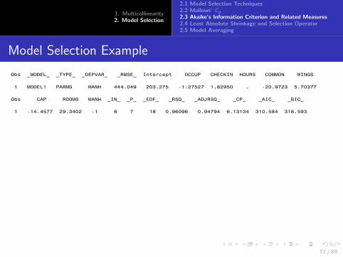
1. Multicollinearity2. Model Selection
2.1 Model Selection Techniques2.2 Mallows’ Cp2.3 Akaike’s Information Criterion and Related Measures2.4 Least Absolute Shrinkage and Selection Operator2.5 Model Averaging
Model Selection Example
Obs _MODEL_ _TYPE_ _DEPVAR_ _RMSE_ Intercept OCCUP CHECKIN HOURS COMMON WINGS 1 MODEL1 PARMS MANH 444.049 203.275 -1.27527 1.82950 . -20.9723 5.70377 Obs CAP ROOMS MANH _IN_ _P_ _EDF_ _RSQ_ _ADJRSQ_ _CP_ _AIC_ _BIC_ 1 -14.4577 29.3402 -1 6 7 18 0.96096 0.94794 6.13134 310.584 318.593
72 / 89

1. Multicollinearity2. Model Selection
2.1 Model Selection Techniques2.2 Mallows’ Cp2.3 Akaike’s Information Criterion and Related Measures2.4 Least Absolute Shrinkage and Selection Operator2.5 Model Averaging
Model Selection Example
proc rsquare data=boq outest=est cp adjrsq aic bic; model manh=occup checkin hours common wings cap rooms; ods select subsetselsummary; run; data est2; set est; if round(_AIC_,0.0001)=310.5841; proc print data=est2; run;
73 / 89

1. Multicollinearity2. Model Selection
2.1 Model Selection Techniques2.2 Mallows’ Cp2.3 Akaike’s Information Criterion and Related Measures2.4 Least Absolute Shrinkage and Selection Operator2.5 Model Averaging
LASSO
I Recall that for ridge regression
bridge = argminβ∈Rk
(Y − Xβ)′(Y − Xβ) + λβ′β
can have better MSE than O.L.S. depending on the choice ofλ.
I But it will never set coefficients to zero exactly, and thereforeit cannot perform model selection.
I While this does not hurt its prediction ability, it is notdesirable for the purpose of interpretation especially for thenumber of coefficients is large.
74 / 89

1. Multicollinearity2. Model Selection
2.1 Model Selection Techniques2.2 Mallows’ Cp2.3 Akaike’s Information Criterion and Related Measures2.4 Least Absolute Shrinkage and Selection Operator2.5 Model Averaging
LASSO
I The LASSO (Tibshirani, 1996) is defined as
blasso = argminβ∈Rk
(Y − Xβ)′(Y − Xβ) + λ||β||
I That is, the LASSO minimises the sum of squared errorssubject to the constraint that the sum of the absolute valuesof βj ’s is smaller than a pre-determined constant.
75 / 89

1. Multicollinearity2. Model Selection
2.1 Model Selection Techniques2.2 Mallows’ Cp2.3 Akaike’s Information Criterion and Related Measures2.4 Least Absolute Shrinkage and Selection Operator2.5 Model Averaging
LASSO
I LASSO is an acronym for Least Absolute Selection andShrinkage Operator.
I Ridge regression uses a squared (l2) penalty, while LASSOuses an absolute (l1) penalty.
I Again, the tuning parameter λ controls the strength of thepenalty, and as in ridge regression, blasso=O.L.S. when= λ = 0 and blasso = 0 when λ =∞.
I For λ that lies between the two extremes, we are balancingthe ideas of fitting a model of Y on X and shrinking thecoefficients.
76 / 89

1. Multicollinearity2. Model Selection
2.1 Model Selection Techniques2.2 Mallows’ Cp2.3 Akaike’s Information Criterion and Related Measures2.4 Least Absolute Shrinkage and Selection Operator2.5 Model Averaging
LASSO
I By the nature of the l1 penalty, some of the coefficients willbe shrunken exactly to zero.
I The ability to perform selection makes the LASSOsubstantially different from Ridge.
I The LASSO problem is usually solved with the columns of Xscaled to have a sample variance of 1; otherwise the penaltyterm is an unfair representation because the regressors are notof the same scale.
77 / 89
1. Multicollinearity2. Model Selection
2.1 Model Selection Techniques2.2 Mallows’ Cp2.3 Akaike’s Information Criterion and Related Measures2.4 Least Absolute Shrinkage and Selection Operator2.5 Model Averaging
LASSO
I The theory and computation of LASSO are complicated andbeyond the scope of this course. The computation of theLASSO solutions is a quadratic programming problem but theLeast Angle Regressions (LARS) algorithm provides a moreefficient way for computing the estimates and is usually usedinstead.
I In SAS, LASSO can be implemented under PROCGLMSELECT. The PARTITION statement randomly reservescertain percentage of data as validation data and uses theremaining the for estimation.
78 / 89

1. Multicollinearity2. Model Selection
2.1 Model Selection Techniques2.2 Mallows’ Cp2.3 Akaike’s Information Criterion and Related Measures2.4 Least Absolute Shrinkage and Selection Operator2.5 Model Averaging
LASSO
I The CHOOSE=VALIDATE suboption requests that validationdata be used for the tuning method for the LASSO selection.
I The observations in the training set are used to produce theLASSO estimates of coefficients and the observations in thevalidation set are used to compute the prediction errors. Themodel that yields the smallest average squared error (ASE)across the observations in the validation set is selected.
I LASSO is more effective when there is a large number ofobservations in the sample.
I Consider the following simulation example where there existfive regressors but only two are contained in the true model.The number of observations is 1000.
79 / 89

1. Multicollinearity2. Model Selection
2.1 Model Selection Techniques2.2 Mallows’ Cp2.3 Akaike’s Information Criterion and Related Measures2.4 Least Absolute Shrinkage and Selection Operator2.5 Model Averaging
LASSO Example
data Simdata; drop i j; array x{5} x1-x5; do i=1 to 1000; do j=1 to 5; x{j} = ranuni(1); end; yTrue = 2 + 5*x2 - 17*x1; y = yTrue + 2*rannor(1); output Simdata; end; run; ods graphics on; proc glmselect data=Simdata plots=ase(stepaxis=normb); partition fraction(validate=.3); model y = x1 x2 x3 x4 x5 / selection=lasso(stop=none choose=validate); run;
80 / 89
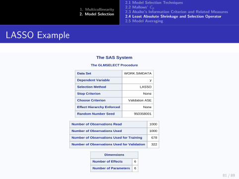
1. Multicollinearity2. Model Selection
2.1 Model Selection Techniques2.2 Mallows’ Cp2.3 Akaike’s Information Criterion and Related Measures2.4 Least Absolute Shrinkage and Selection Operator2.5 Model Averaging
LASSO ExampleSAS Output
SAS Output_htm#IDX9.htm[11/7/2016 3:25:22 PM]
The SAS System
The GLMSELECT Procedure
Data Set WORK.SIMDATA
Dependent Variable y
Selection Method LASSO
Stop Criterion None
Choose Criterion Validation ASE
Effect Hierarchy Enforced None
Random Number Seed 950358001
Number of Observations Read 1000
Number of Observations Used 1000
Number of Observations Used for Training 678
Number of Observations Used for Validation 322
Dimensions
Number of Effects 6
Number of Parameters 6
81 / 89

1. Multicollinearity2. Model Selection
2.1 Model Selection Techniques2.2 Mallows’ Cp2.3 Akaike’s Information Criterion and Related Measures2.4 Least Absolute Shrinkage and Selection Operator2.5 Model Averaging
LASSO ExampleSAS Output
SAS Output_htm#IDX9.htm[11/7/2016 3:25:22 PM]
The SAS System
The GLMSELECT Procedure
LASSO Selection Summary
StepEffectEntered
EffectRemoved
NumberEffects In ASE
Validation ASE
0 Intercept 1 29.5677 30.3995
1 x1 2 8.8482 9.0758
2 x2 3 3.9141 4.5750*
3 x5 4 3.8944 4.5980
4 x3 5 3.8937 4.5995
5 x4 6 3.8784 4.6597
* Optimal Value Of Criterion
Selection stopped because all effects are in the final model. 82 / 89

1. Multicollinearity2. Model Selection
2.1 Model Selection Techniques2.2 Mallows’ Cp2.3 Akaike’s Information Criterion and Related Measures2.4 Least Absolute Shrinkage and Selection Operator2.5 Model Averaging
LASSO Example
83 / 89

1. Multicollinearity2. Model Selection
2.1 Model Selection Techniques2.2 Mallows’ Cp2.3 Akaike’s Information Criterion and Related Measures2.4 Least Absolute Shrinkage and Selection Operator2.5 Model Averaging
LASSO ExampleSAS Output
SAS Output_htm#IDX9.htm[11/7/2016 3:25:22 PM]
The SAS System
The GLMSELECT ProcedureSelected Model
The selected model, based on Validation ASE, is the model at Step 2.
Effects: Intercept x1 x2
Analysis of Variance
Source DFSum of
SquaresMean
Square F Value
Model 2 17393 8696.55920 2212.02
Error 675 2653.76121 3.93150
Corrected Total 677 20047
Root MSE 1.98280
Dependent Mean -3.70715
R-Square 0.8676
Adj R-Sq 0.8672
AIC 1611.18927
AICC 1611.24871
SBC 944.74672
ASE (Train) 3.91410
ASE (Validate) 4.57499
Parameter Estimates
Parameter DF Estimate
Intercept 1 1.658314
x1 1 -16.517352
x2 1 5.234656
84 / 89

1. Multicollinearity2. Model Selection
2.1 Model Selection Techniques2.2 Mallows’ Cp2.3 Akaike’s Information Criterion and Related Measures2.4 Least Absolute Shrinkage and Selection Operator2.5 Model Averaging
LASSO
I There has been an explosion of research activities related tothe LASSO and its variants. Generalisations of LASSO includethe Adaptive LASSO that uses adaptive weights in penalisingthe coefficients; the elastic net (EN) which can handlesituations when k > n; when a group of variables exhibitstrong correlations, the EN will select the discard the entiregroup; the Octagon shrinkage and clustering algorithm forregression (OSCAR) method which can deliver the samecoefficient estimate for regressors whose relationships with theresponse are similar, etc. etc.
85 / 89
1. Multicollinearity2. Model Selection
2.1 Model Selection Techniques2.2 Mallows’ Cp2.3 Akaike’s Information Criterion and Related Measures2.4 Least Absolute Shrinkage and Selection Operator2.5 Model Averaging
Model Averaging
I There are several problems associated with model selection:I Because of sampling fluctuations it is highly unlikely for the
best fitting model in one sample to be the preferred modelacross all samples, especially when the data generating processis associated with a very high noise level. This points towardsa replication crisis, referred to as the inability to replicateresults (or generalise findings) obtained in a single sampleacross situations.
I Model selection is a random event. It can lead to a very poormodel being chosen and all subsequent predictions and analysisare contingent on this model.
I Inference is also contingent on the chosen model, assumingthat it is known in advance without recognising that therandomness associated with model selection.
86 / 89
1. Multicollinearity2. Model Selection
2.1 Model Selection Techniques2.2 Mallows’ Cp2.3 Akaike’s Information Criterion and Related Measures2.4 Least Absolute Shrinkage and Selection Operator2.5 Model Averaging
Model Averaging
I In recent years, model selection has gradually evolved intomodel averaging
I Instead of choosing one model, model averaging combinesestimates from an ensemble of models, using weights thatreflect the extent to which the different models are supportedby the data.
I There are two central questions to model averaging:I How to form weights? Many methods have been proposed
based on information criterion scores, Mallows Cp,cross-validation, etc., oriented towards achieving optimality ofsome forms.
I How to draw inference based on a model average? One needsinformation on the distributions of model average estimators
87 / 89

1. Multicollinearity2. Model Selection
2.1 Model Selection Techniques2.2 Mallows’ Cp2.3 Akaike’s Information Criterion and Related Measures2.4 Least Absolute Shrinkage and Selection Operator2.5 Model Averaging
Model Averaging
I There has been an explosion of research into the above inrecent years
I Smoothed-AIC (S-AIC) and Smoothed-BIC (S-BIC) weights,by which
wm =exp{−xICm/2}∑M
m=1 exp{−xICm/2}, (1)
where xICm is the AIC or BIC score of the mth model. Thisweighting scheme is justified by noting that for the S-AIC, theratio in (1) is the relative penalised likelihood factor, and forthe S-BIC, it is Schwarz’s (1978) approximation to the Bayesfactor.
I M = 2p, the maximum number of candidate models
88 / 89

1. Multicollinearity2. Model Selection
2.1 Model Selection Techniques2.2 Mallows’ Cp2.3 Akaike’s Information Criterion and Related Measures2.4 Least Absolute Shrinkage and Selection Operator2.5 Model Averaging
Model Averaging
I So the final estimate of a parameter is formed by a weightedcombination of the estimates obtained in different models.
I That is, βMA =∑M
m=1 wmβm
I Model averaging does not always improve over modelselection. Typically when the underlying process has a smallnoise content, selection is a better strategy than averaging,and vice versa.
I However, usually when selection is a superior strategy,averaging is only marginally worse, but when averaging issuperior, it is often a better strategy by a large margin. Why ?
89 / 89