Chapter 4

Characterizing Data Numerically: Descriptive Statistics

While visual representations of data are very useful, they are only a beginning

point from which we may gain more information. Numerical characterizations allow a

more formal means of both describing a distribution and comparing two or more

distributions. Numerical description ultimately allows us to make the inferences we

desire. These numerical characterizations are termed either statistics or parameters.

Statistics are descriptions of the constructed characteristics of a sample, whereas

parameters refer to the characteristics of a population. A population is a group of data

defined in time and space. Do not confuse this use of the term population with its use in

biology and physical anthropology. Statistical populations are not things. They are not

people, or animals, or rocks, or pots. They are data.

For example, the length of Folsom points manufactured during the Paleoindian

occupation of the New World could be considered a population. The size of thimbles

used in New York during the Historic period is another possible population. As you can

see populations can vary in their scope from data about all of a class of objects ever in

existence to data on a more limited subset of objects. We could even define a population

at the scale of a site (e.g., the frequencies of each species of animals consumed at a site

could be considered a population.)

In contrast a sample is a subset of a population that does not contain all of the

population’s members. For example, the animals reflected by bones recovered from a site

4-1

is a sample of the population of all of the animals consumed at a settlement. A point to

remember is that the archaeologist defines populations and samples. Samples and

populations are not discovered. A particular group of data could be a sample or a

population, depending on your question. For example the grade point average of

undergraduate anthropology majors at a school could be considered a population, if the

group of interest is anthropology majors from that school, or a sample, if you are

interested in all undergraduates from the institution.

We generally analyze a sample to gain information about the population. We

therefore often use sample statistics to make inferences about population parameters of

interest. For example, we may numerically characterize the cranial capacity of a sample

of australopithecine skulls. This characterization may be in terms of one or more

statistics. We then use the statistics derived from a sample to infer information about the

population of australopithecine skulls of interest.

It is important to remember that statistics may vary, as each is likely a description

derived from a different subset of a population. Parameters, however, do not vary,

because they are a description of a complete population bounded in space and time. They

are unchanging, immutable.

Numerical descriptions of distributions can be categorized into two types:

measures of central tendency, and measures of dispersion. Measures of central tendency,

as the name suggests, provide a numerical account of the center, or midpoint of a

distribution. Measures of dispersion provide information about the spread of data around

the midpoint of the distribution. Both populations and samples can be characterized using

4-2

measures of central tendency and dispersion. By convention, population parameters are

denoted with Greek letters, and sample statistics by Roman letters.

MEASURES OF CENTRAL TENDENCY

Measures of central tendency are often referred to as well as measures of location.

Measures of location may actually be the better term, in that these measures provide a

numerical account of the location of the center of a distribution along the variable

measured.

Three measures of central tendency are commonly used: the median, the mean,

and the mode.

Median

The median of a set of data is the variate with the same number of observations of

both greater and lesser value. Consider the following scaled list of variates:

14, 15, 16, 19, 23

The variate 16 is bounded on both sides by two variates. The median value is

therefore 16. Consider an additional set of scaled variates that consist of an even number:

14, 15, 16, 19

Unlike the example above, no single number has an equal number of variates

numerically greater and less than it. So how do we decide what the median is? Is it 15 or

16, or does this set of numbers simply have no median? In cases such as this, the median

4-3

is determined by averaging the two values in the middle of the distribution. Here, the

median is the average of 15 and 16, which is 15.5.

Mode

The mode is the most popular, or most abundant value, in a data set (i.e., the value with

the highest frequency). An inspection of Figure 3.7 (Chapter 3) shows that the most

popular value in the Gallina ceramic data is 5.0. It is possible, though, to have two or

more modes, if the most popular classes have the exact same number of variates.

Mean

Everyone is familiar with this measure of central tendency, which is also called the

arithmetic mean, or the average. The mean is calculated by summing all of the values in

the set of data, and then dividing this sum by the number of observations.

To illustrate the calculation of the mean, consider the following set of data (Table

4.1) Jim O'Connell collected in an ethnoarchaeological study on the number of residents

in Alyawara camps.

Table 4.1. Number of residents in Alyawara camps. 21 23 18 31 12 44 31 7

4-4

The mean is calculated by following the instructions in the following symbols

presented in Equation 4.1.

Equation 4.1. Calculating the mean.

n

Yni

ii∑

=

== 1µ or, more simply, nY∑

In equation 4.1, µ represents the population parameter of the mean of the

variable Y. Y (vocalized as Y-bar) is the mean of a sample, and is an estimate of µ . In

this case, Y refers to the mean of the number of residents of Alyawara camps. The Greek

symbol ∑ should be familiar from Chapter 3 as the symbol for summation. What might

not be familiar however, is the notation above and below ∑, and the subscript to the right

of Y.

∑=

=

ni

1iiY represents the following set of instructions: for the variable Y, beginning

with the first value of Y (symbolized by i=1), sum all values continuing to the last value

of Y (symbolized by i=n). simply refers to all values of Y, each of which can be

numbered individually, as follows:

iY

7Y...12Y,18Y,21Y 8321 ==== . For the set of

instructions ∑ we begin summation with =

=

4i

2iiY 18Y2 = , and continue to sum through

, or 18 + 12 + 31 = 61. 31Y4 =

4-5

The left term of Equation 4.1 shows the full symbolism for the calculation of the

mean. The term on the right means the same thing, all other symbolism associated with

the term to the left is implied. Seldom is the full symbolism expressed for ease of

application. So, when you encounter the symbol ∑Y, it can be assumed that the

instructions are to sum all values of Y, beginning with the first, and continuing to the last.

The calculation of the mean in our Alyawara example is as follows.

8744312331121821 +++++++

=Y

8187

=Y

37523.Y =

The mean, or average number of Alyawara's in camp is 23.375. The median is 22,

and the mode, 31. Depending upon the situation, all three measures may be useful, but

oftentimes, one may be preferred over the others. In the above example, the mean and the

median provide values that are reasonably close to one another, and both constitute good

measures of central tendency. The mode in this instance, however, is inaccurate as a

measure of central tendency, probably because the sample size is so small.

When a distribution is perfectly symmetrical, the mode, mean, and median are

identical. In general, when dealing with a symmetrical distribution, the mean is the most

useful measure of central tendency, followed by the median, and then the mode. The

4-6

mean is often the most useful primarily because of its utility in the analysis of variance

and regression analysis, subjects of later chapters. The mean, however, can be innately

influenced by extreme values, often called outliers. As a result, its applicability to heavily

skewed distributions is questionable.

For example consider again the following values for the Alyawara data:

21, 18, 12, 31, 23, 31, 44, 7

Let us replace the variate 44 in the above data with 100, as illustrated in the following set

of contrived data.

21, 18, 12, 31, 23, 31, 100, 7

In comparison with 37523.Y = for the original set of data, the recalculation off

the mean with the extreme value of 100 provides us with a value of 37530.Y = , a

considerable increase. The median, however, is unaffected by the extreme value, and

remains the same. It is in such cases as where extreme values exist, or where the data are

heavily skewed, that the median becomes a better indicator of central tendency than the

mean.

MEASURES OF DISPERSION

4-7

While measures of central tendency provide important information about the

location of a distribution along a variable, they offer no information about the shape of

that distribution. Two different distributions might have the same location, but not

resemble each other at all in terms of shape, or dispersion (e.g., Figure 4.1). Three

measures of dispersion are commonly used: the range, the variance, and the standard

deviation.

Range

The range is the difference between the largest and smallest values in a set of

data. For the Alyawara example:

Largest Value 44

Smallest Value (-)7

Range 37

While the range allows a perspective on the dispersion of the distribution of a

sample, the sample range almost always underestimates the population parameter. It is

unlikely, after all, that both the absolute largest and absolute smallest variates in a

population will be selected in most samples. Likewise, the range is greatly affected by

outliers because it only takes into account two variates in the data set, the largest and

smallest.

4-8

Despite the simplicity of the range, it is often a misunderstood statistic because of

the differential use of the verb and noun forms of the word range. With the Alyawara

data, it is appropriate to state that the data range (verb form) from 7 to 44. However, the

range (noun form) is 37, not 7 to 44.

Interquartile Range

Interquartile range is a measure of variation that is closely related to the range,

except that it attempts to measure the variation in variates towards the center of a

distribution. It is calculated by subtracting the variate demarcating the lower 25% of a

distribution from the variate demarcating the upper 25% of the distribution. This value in

turn reflects the range of the middle 50% or the “body” of a distribution. To prevent

confusion, the demarcation of the lower 25% of the distribution is called the 25th

percentile whereas the demarcation of the upper 25% is called the 75th percentile.

Using the Alyawara data, 25% of the variates are equal to or less than 18 and 25%

are equal to or greater than 31. Consequently the 25th percentile is 18 and the 75th

percentile is 31. The interquartile range is 31 – 18 = 13. Thus, the middle 50% of the

Alyawara data differ by no more than 13 people.

Variance and Standard Deviation

4-9

The variance and the standard deviation are related statistics used to describe, and

ultimately compare, the shapes of distributions. Ideally, the value of every single variate

should be considered when characterizing the shape of the distribution. Information about

the shape of the distribution is contained in knowledge of the value, or location of every

variate in space. A logical way to measure the distribution of variates to characterize the

distribution’s shape is to consider the distance, or deviation, of each value from the mean.

For , the distance or deviation from the mean is: 21Y1 =

Yy −= 1Y

3752321 .y −=

3752.y −=

Note that the lower case y is used as the symbol of this deviation, and by

convention, the mean is subtracted from the variate in order to provide the measure of

distance. Yet, this is only one value, and we are concerned with the shape of the complete

distribution. It comes to mind that perhaps if we sum all of the deviations of all variates

from the mean, and divide by the number of variates, we could create a kind of "average"

deviation. Large values would indicate a broadly spread distribution, and small values a

narrowly spread distribution. Unfortunately, this is not the case, as the sum of all

deviations from the mean is equal to zero. Because of the way the mean is calculated, the

amount of deviation is equal on either side and, therefore, the values greater and lesser

than the mean wind up canceling each other out when summed. The problem then, is not

4-10

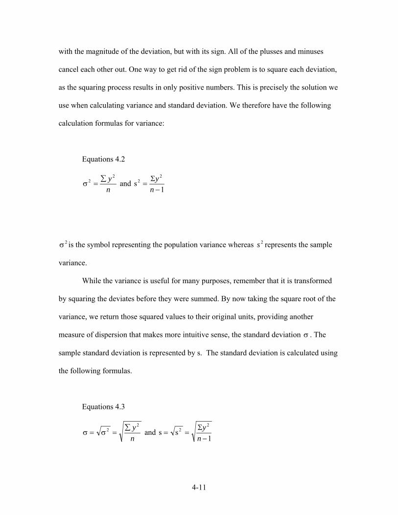
with the magnitude of the deviation, but with its sign. All of the plusses and minuses

cancel each other out. One way to get rid of the sign problem is to square each deviation,

as the squaring process results in only positive numbers. This is precisely the solution we

use when calculating variance and standard deviation. We therefore have the following

calculation formulas for variance:

Equations 4.2

ny 2

2 ∑=σ and

1s

22

−Σ

=n

y

2σ is the symbol representing the population variance whereas represents the sample

variance.

2s

While the variance is useful for many purposes, remember that it is transformed

by squaring the deviates before they were summed. By now taking the square root of the

variance, we return those squared values to their original units, providing another

measure of dispersion that makes more intuitive sense, the standard deviation . The

sample standard deviation is represented by s. The standard deviation is calculated using

the following formulas.

σ

Equations 4.3

ny 2

2 ∑=σ=σ and

1ss

22

−Σ

==n

y

4-11

You will notice that the sample variance and sample standard deviation are

calculated by dividing the sum of squares by n-1, not n. Through experimentation, it has

been determined that dividing by n in a sample tends to underestimate the true variance

and standard deviation, but that dividing by n-1 provides a better estimate. Therefore,

when calculating the population parameters of σ or , divide the sum of squares by n,

but when calculating s or s², divide the sum of squares by n-1.

2σ

Table 4.2 presents in table form the computation of the sample variance and

standard deviations for the Alyawara example.

Table 4.2. Computations of the Sample Variance and Standard Deviation for the Number of Residents in Alyawara Camps.

(1) (2) (3) (4) (5)

Y F Yy -Y = y² fy²

21 1 -2.375 5.641 5.641

18 1 -5.375 28.891 28.891

12 1 -11.375 129.391 129.391

31 2 7.625 58.141 116.281

23 1 -.375 0.141 .141

44 1 20.625 425.391 425.391

7 1 -16.375 268.141 268.141

Sum= 8 0 973.877

37523.Y =

4-12

∑ = 8779732 .y

1251397877973

1s

22 ..

ny

==−

Σ=

795111251391

s2

..n

y==

−Σ

=

Column (1) of Table 4.2 presents each Y. Column (2) presents their frequency f.

This column is necessary because the frequency of occurrence of a given Y may vary. If

we counted each Y with multiple occurrences only once, we would either overestimate or

underestimate the true variance. Column (3) presents y, Y-Y , the deviation of the

variate from the mean. Note, as discussed above, the sum of all values in column (3) is

equal to zero. Column (4) provides a solution to the problem with signs by squaring the

deviations created in column (3) as symbolized by . Column (5) is the frequency of

occurrence of Y as presented in Column (2) multiplied by the squared deviations

calculated in column (4). This column is necessary in order to take into account the Y's

with more than one observation. The sum of column (5) ∑ f =973.877 is also called the

sum of squares. This value is then used in Equations 4.2 and 4.3.

2y

2y

The procedure illustrated in Table 4.2 is a useful approach to calculating the

sample variance and standard deviation, but it does take some effort to produce. One of

the most pleasant characteristics of statistics is that there are often simple ways to

calculate otherwise complex calculations. Equation 4.4 offers an equivalent method of

4-13

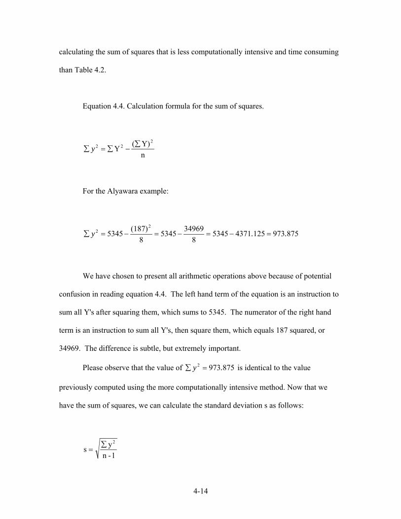
calculating the sum of squares that is less computationally intensive and time consuming

than Table 4.2.

Equation 4.4. Calculation formula for the sum of squares.

nY)(Y

222 ∑−∑=∑ y

For the Alyawara example:

875973125437153458

3496953458

(187)53452

2 ..y =−=−=−=∑

We have chosen to present all arithmetic operations above because of potential

confusion in reading equation 4.4. The left hand term of the equation is an instruction to

sum all Y's after squaring them, which sums to 5345. The numerator of the right hand

term is an instruction to sum all Y's, then square them, which equals 187 squared, or

34969. The difference is subtle, but extremely important.

Please observe that the value of is identical to the value

previously computed using the more computationally intensive method. Now that we

have the sum of squares, we can calculate the standard deviation s as follows:

8759732 .y =∑

1-nys

2∑=

4-14

7973.875s =

11.795s =

With knowledge of the standard deviation, we now have obtained an extremely

useful measure of dispersion. In addition, principles behind the calculation of the

standard deviation provide extremely important conceptual tools for understanding many

statistics we will be learning through the remainder of this book.

Calculating Estimates of the Mean and Standard Deviation

Occasionally, we are faced with situations where we wish to quickly gain

information about the location and spread of a distribution; for example, at a professional

presentation where we want to explore some relationship in data being presented. We

may also wish to quickly check our mean and standard deviation calculations for possible

errors without actually recomputing the values. Using the following procedures, we can

calculate a quick estimate of both the mean and the standard deviation.

To estimate the mean, we can compute the midrange. The midrange is similar to

the range except that the largest and smallest values are averaged rather than subtracted.

4-15

In the Alyawara example, the midrange is (44+7)/2 = 25.5. This value is fairly close to

the computed mean of 23.375 and may serve as a reasonable estimate. If the midrange is

very different, one may want to recheck the computation of the mean.

While estimates of the mean are easy to come by, a good estimate of the standard

deviation is a bit more difficult. However, the standard deviation can be estimated by

dividing the range, calculated as described previously, with the appropriate value from

Table 4.3. Applying this method to the Alyawara example produces an estimate of (37/3)

= 12.3. Once again, this value is not too far off from the computed value of s = 11.795.

Table 4.3. Denominators for the estimate of the standard deviation.

Sample Size Divide Range By

5 to 29 3

30 to 99 4

100 to 499 5

500 to 999 6

1000+ 6.5

Coefficients of Variation

Oftentimes we calculate standard deviations because our goal is to compare the

spread of two or more distributions. In such cases distributions with larger variances and

standard deviations relative to other distributions are thought to reflect populations with

greater variation. This assumption is seems intuitively obvious but is in fact problematic

because we must first recognize that the variance and standard deviation are strongly

influenced by the size of the variable being measured. For example, Clovis projectile

4-16

points tend to be much longer than projectile points used by those living in the proto-

historic pueblos in the American Southwest. If the standard deviation were used to

compare the amount of variation in the lengths of the two types of points, it would be

calculated for each type using the sums of deviations of each variate from the group

mean. The standard deviation for the proto-historic points consequently will always be

smaller than the corresponding standard deviation for Clovis points because the proto-

historic points are themselves smaller. Each proto-historic projectile point variate cannot

differ at the same magnitude from its mean as a Clovis point variate can. As a result the

standard deviation and variance are inappropriate for comparing the relative amount of

variation within two or more groups when group means are significantly different,

because they will tend to overestimate the amount of variation in large variables and

underestimate the amount of variation in smaller variables relative to each other.

This problem is resolved by calculating the coefficient of variation. The

coefficient of variation (CV) is an expression of the standard deviation as a percentage of

the mean from the parent distribution. It standardizes the standard deviation so that the

absolute size of the variable being measured is controlled. Instead of reflecting the

absolute size of the variation from the mean, CVs reflect the proportion of variation from

the mean. Thus, a Clovis point and a proto-historic projectile point that are two thirds of

their respective mean lengths will demonstrate the same proportional variation as

determined by the CV. The CV therefore allows the variation within distributions with

significantly different means to be compared. The coefficient of variation is computed

using equation 4.6.

4-17

Equation 4.6. The Coefficient of Variation

Y100*scv = for samples, or

µσ

=100*cv for populations

For the Alyawara example:

50.46 23.375

100 * 11.795 cv ==

The coefficient of variation has meaning only in a comparative sense to another

coefficients of variation. For example, we might be interested in comparing the variation

in camp sizes of the Alyawara with another group with 8 n 12, s 30, Y === . For this

second group:

4030

100*12cv ==

Since 50.46 > 40, the Alyawara variation is greater than that of the second group.

It has been determined that the cv is a biased estimate of the population parameter

in small samples. We therefore apply a correction term to eliminate the bias. The

corrected coefficient of variation (corrected cv or cv*) is computed using Equation 4.7.

Equation 4.7. Correction formula for the coefficient of variation.

4-18

cv )n41 (1 *cv +=

For the Alyawara example:

)50.46(8)41 (1 *cv +=

cv* = 52.04

For the second group:

)40(8)41 (1 *cv +=

cv* = 41.25

Our conclusions regarding the variation in our Alyawara example are the same,

since 52.04 > 41.25, yet we now likely have better estimates of the parametric values.

Coefficients of variation are commonly used where comparisons of standard

deviations are desired, particularly where means differ considerably. For example, to

compare variation in the skeletal morphology of different primate groups who vary

significantly in size, the comparison of coefficients of variation is necessary.

4-19

Another common application is where researchers are interested in examining

specialized production of technology. Lower coefficients of variation suggest greater

standardization of products, and may mean specialized production. Coefficients of

variation have been employed by Crown (1995), Longacre et al (1988), and others (e.g.,

Arnold and Nieves 1992; Mills 1995) as a measure of standardization. Crown notes that

with respect to the manufacture of ceramics, known specialist groups rarely produce

ceramics with coefficients of variation above 10%. Her examination of variation in

Salado Polychromes in the American Southwest allows her to conclude that there was

little, if any, standardization and subsequently little, if any, specialized production.

Box Plots

Now that we have an understanding of the median and the range we can employ

an addition means of visually characterizing data, box plots. Box plots are extremely

useful for characterizing multiple distributions at the same time, although they can be

used for even a single distribution, because they provide information about the variation

and central tendencies of data in a very condensed manner (e.g., Figure 4.2).

Box plots reflect the median, the interquartile, and the range. They are created in

three steps. First, calculate the distribution’s median and the quartiles. Second, plot the

location of the median and the two quartiles. Draw a box using the quartiles as limits.

This box reflects the distribution of the middle 50% of the data—the “body” of the data.

Third, draw a line from the lower quartile to the value of the smallest variate and from the

upper quartile to the value of the largest variate.

4-20

The utility of box plots can be demonstrated in Figure 4.2. This figure is the

length of 4 sets of 12 flakes made as part of an experiment studying of the flaking

characteristics of lithic raw materials (Table 4.XX). The box plots in Figure 4.2 provide a

quick means of describing both the structure of each distribution and the differences

between them.

Figure 4.2. Box plots of flake length data presented in Table 4.XX.

12121212N =

QuartziteObsidianChertBasalt

16

14

12

10

8

6

4

2

0

4-21

Table 4.XX. Flake length by raw material.

Basalt Chert Obsidian Quartzite7.0 2.9 2.2 5.5 7.0 4.8 2.4 5.5 7.7 5.3 3.1 7.0 8.2 5.8 4.3 7.4 10.3 5.8 5.0 7.7 10.3 6.2 5.5 7.9 10.3 6.5 5.8 8.6 10.8 7.7 6.0 8.9 11.0 7.7 6.2 9.4 13.0 7.9 7.2 9.6 13.9 8.9 7.4 10.6 14.6 9.6 7.7 10.8

We now know how to characterize data visually and numerically. The next step is to

learn one important theoretical distribution, the normal distribution. Knowledge of the

characteristics of the normal distribution allows us to draw conclusions about real

distributions that take a similar form. The normal distribution is the subject of Chapter 5.

Figure 4.1. Two distributions with identical means and sample sizes but different dispersion patterns.

0

5

10

15

20

0

5

10

15

20

4-22

12121212N =

QuartziteObsidianChertBasalt

16

14

12

10

8

6

4

2

0

4-23