chapter 4 lagrangian mechanics - department of physics...

Chapter 4

Lagrangian mechanics

Motivated by discussions of the variational principle in the previous chapter,together with the insights of special relativity and the principle of equivalencein finding the motions of free particles and particles in uniform gravitationalfields, we seek now a variational principle for the motion of nonrelativisticparticles subject to arbitrary forces. This will lead us to introduce Hamil-ton’s principle and the Lagrangian to describe physical systems in me-chanics, both for single particles and systems of particles. These conceptstogether are so elegant that we are encouraged to place them at the veryheart of classical mechanics. We are further encouraged to do so in the fol-lowing chapter, the capstone chapter to Part I of the book, where we showhow they naturally emerge as we take the classical limit of the vastly morecomprehensive theory of quantum mechanics.

4.1 The Lagrangian in Cartesian coordinates

At the end of Chapter 3 we reached the intriguing conclusion that the correctequations of motion for a nonrelativistic particle of mass m in a uniformgravitational field can be found by making stationary the functional

I →∫dt

(1

2mv2 − U

)=

∫dt (T − U), (4.1)

where

T ≡ 1

2mv2 (4.2)

139

4.1. THE LAGRANGIAN IN CARTESIAN COORDINATES

is the particle’s kinetic energy and

U = mgy (4.3)

is its gravitational potential energy. It was the difference between the kineticand gravitational potential energy that was needed in the integrand.

Now suppose that a particle is subject to an arbitrary conservative forcefor which a potential energy U can be defined. Does the form

I →∫dt

(1

2mv2 − U

)=

∫dt (T − U) (4.4)

still work? Do we still get the correct F = ma equations of motion?Let us do a quick check using Cartesian coordinates. Note that if U =

U(x, y, z) and T = T (x, y, z), then the integrand in the variational problem,which we now denote by the letter L, is

L(x, y, z, x, y, z) ≡ T (x, y, z)− U(x, y, z) =1

2mv2 − U(x, y, z), (4.5)

where v2 = x2 + y2 + z2. Writing out the three associated Euler equations,we get the differential equations of motion

∂L

∂x− d

dt

∂L

∂x= 0,

∂L

∂y− d

dt

∂L

∂y= 0,

∂L

∂z− d

dt

∂L

∂z= 0, (4.6)

where

∂L

∂x= −∂U

∂x= Fx and

d

dt

∂L

∂x=

d

dtmx = mx, so Fx = mx, (4.7)

with similar results in the y and z directions. That is, we have derived thethree components of F = ma,

Fx = mx, Fy = my, Fz = mz ⇒ −∇U = ma . (4.8)

The quantity

L = T − U (4.9)

is called the Lagrangian of the particle. As we have seen, using the La-grangian as the integrand in the variational problem gives us the correctequations of motion, at least in Cartesian coordinates, for any conservativeforce!

140

CHAPTER 4. LAGRANGIAN MECHANICS

4.2 Hamilton’s principle

We now have an interesting proposal at hand: reformulate the equations ofmotion of nonrelativistic mechanics, F = dp/dt, in terms of a variationalprinciple making stationary a certain functional. This has two benefits:

(1) It is an interesting and intuitive idea to think of dynamics as arisingfrom making a certain physical quantity stationary; we will appreciate someof these aspects in due time, especially when we get to the chapter on theconnections between classical and quantum mechanics;

(2) This reformulation provides powerful computational tools that can allowone to solve complex mechanics problems with greater ease. The formalismalso lends itself more transparently to implementations in computer algo-rithms.

The Lagrange technique makes brilliant use of what are called generalizedcoordinates, particularly when the particle or particles are subject to oneor more constraints. Suppose that a particular particle is free to move inall three dimensions, so three coordinates are needed to specify its position.The coordinates might be Cartesian (x, y, z), cylindrical (r, ϕ, z), spherical(r, θ, ϕ), as illustrated in Figure 4.1, or they might be any other complete setof three (not necessarily orthogonal) coordinates.1

A different particle may be less free: it might be constrained to moveon a tabletop, or along a wire, or within the confines of a closed box, forexample. Sometimes the presence of a constraint means that fewer thanthree coordinates are required to specify the position of the particle. Soif the particle is restricted to slide on the surface of a table, for example,only two coordinates are needed. Or if the particle is a bead sliding along africtionless wire, only one coordinate is needed, say the distance of the beadfrom a given point on the wire. On the other hand, if the particle is confinedto move within a closed three-dimensional box, the constraint does not reducethe number of coordinates required: we still need three coordinates to specify

1Note that in spherical coordinates the radius r is the distance from the origin, while incylindrical coordinates r is the distance from the vertical (z) axis. Because these r’s refer todifferent distances, some people use ρ instead of r in cylindrical coordinates to distinguishit from the r in spherical coordinates. However, retaining the symbol r in cylindricalcoordinates has the great advantage that on any z = constant plane the coordinates (r, ϕ)automatically become a good choice for conventional planar polar coordinates.

141

4.2. HAMILTON’S PRINCIPLE

Cylindrical SphericalCartesian

FIGURE 4.1 : Cartesian, cylindrical, and spherical coordinates

the position of the particle inside the box.

A constraint that reduces the number of coordinates needed to specifythe position of a particle is called a holonomic constraint. The requirementthat a particle move anywhere on a tabletop is a holonomic constraint, forexample, because the minimum set of required coordinates is lowered fromthree to two, from (say) (x, y, z) to (x, y). The requirement that a beadmove on a wire in the shape of a helix is a holonomic constraint, because theminimum set of required coordinates is lowered from three to one, from (say)cylindrical coordinates (r, ϕ, z) to just z. The requirement that a particleremain within a closed box is nonholonomic, because a requirement thatx1 ≤ x ≤ x2, y1 ≤ y ≤ y2, z1 ≤ z ≤ z2 does not reduce the number ofcoordinates required to locate the particle.

For an unconstrained particle, three coordinates are needed; or if there isa holonomic constraint the number of coordinates is reduced to two or one.We call a minimal set of required coordinates generalized coordinatesand denote them by qk, where k = 1, 2, 3 for a single particle (or k = 1, 2,or just k = 1, for a constrained particle). For each generalized coordinatethere is a generalized velocity qk = dqk/dt. Note that a generalized velocitydoes not necessarily have the dimensions of length/time, just as a generalizedcoordinate does not necessarily have the dimensions of length. For example,the polar angle θ in spherical coordinates is dimensionless, and its generalizedvelocity θ has dimensions of inverse time.

142


Having chosen a set of generalized coordinates qk for a particle, the inte-grand L in the variational problem, where L is called the Lagrangian, canbe written2

L = L(t, q1, q2, .., q1, q2, ...) = L(t, qk, qi) (4.10)

in terms of the generalized coordinates, generalized velocities, and the time.We can now present a more formal statement of the Lagrangian approach

to finding the differential equations of motion of a system.Given a mechanical system described through N dynamical generalized

coordinates labeled qk(t), with k = 1, 2, . . . , N , we define its action S[qk(t)]as the functional of the time integral over the Lagrangian L(t, q1, q2, ..., q1, q2, ...),from a starting time ta to an ending time tb,

S[qk(t)] =

∫ tb

ta

dt L(t, q1, q2, ..., q1, q2, ...) ≡∫ tb

ta

dt L(t, qk, qk) . (4.11)

It is understood that the particle begins at some definite position (q1, q2, ...)aat time ta and ends at some definite position (q1, q2, ...)b at time tb. We thenpropose that, for trajectories qk(t) where S is stationary — i.e., , when

δS = δ

∫ tb

ta

L(t, qk, qk) dt = 0 (4.12)

the qk(t)’s satisfy the equations of motion for the system with the prescribedboundary conditions at ta and tb. This proposal was first enunciated by theIrish mathematician and physicist William Rowan Hamilton (1805 – 1865),and is called Hamilton’s principle.3 From Hamilton’s principle and ourdiscussion of the previous chapter, we get the N Lagrange equations

d

dt

∂L

∂qk− ∂L

∂qk= 0. (k = 1, 2, . . . , N) (4.13)

2Here, we are assuming that the Lagrangian does not involve dependence on higherderivatives of qk, such as qk. It can be shown that such terms lead to differential equationsof the third or higher orders in time (See Problems section). Our goal is to reproducetraditional Newtonian and relativistic mechanics involving differential equations that areno higher than second order.

3It is also sometimes called the Principle of Least Action or the Principle of StationaryAction. This can be confusing, however, because there is an older principle called the“principle of least action” that is quite different.

143


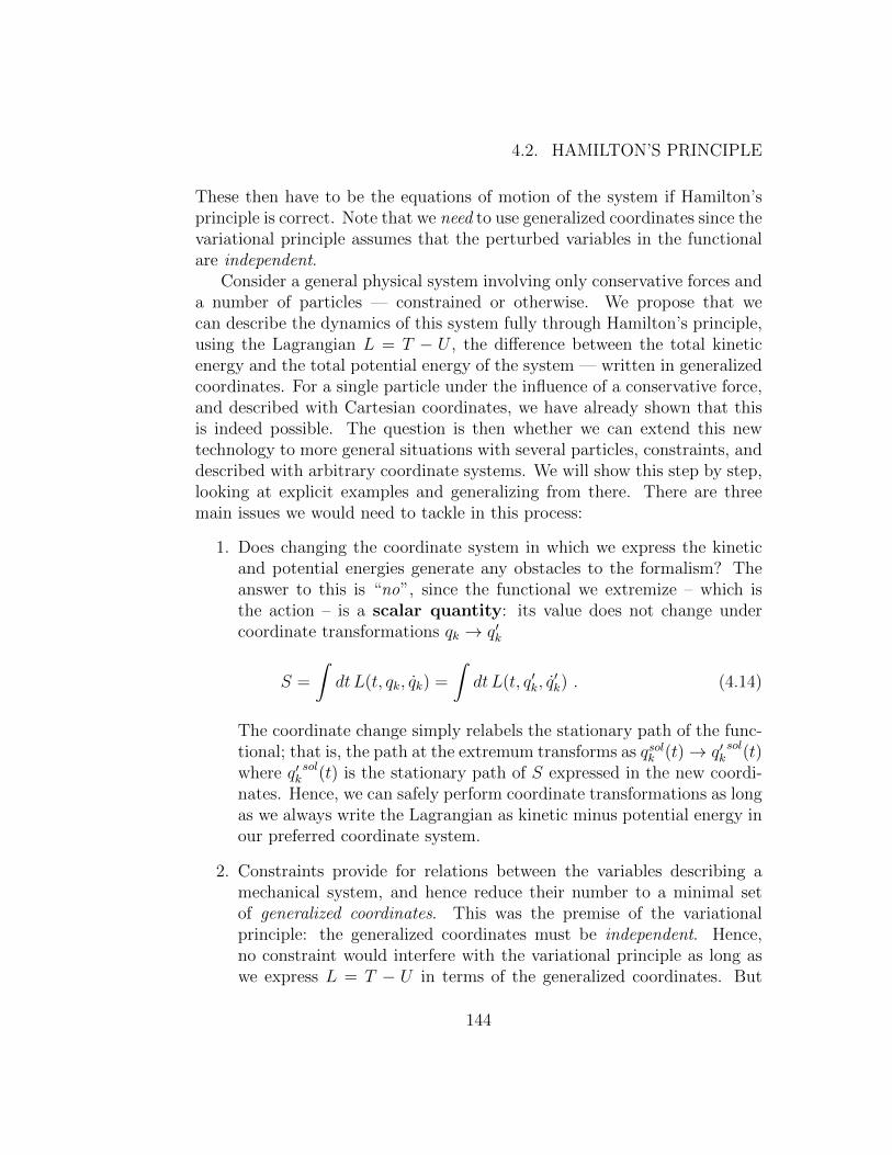
These then have to be the equations of motion of the system if Hamilton’sprinciple is correct. Note that we need to use generalized coordinates since thevariational principle assumes that the perturbed variables in the functionalare independent.

Consider a general physical system involving only conservative forces anda number of particles — constrained or otherwise. We propose that wecan describe the dynamics of this system fully through Hamilton’s principle,using the Lagrangian L = T − U , the difference between the total kineticenergy and the total potential energy of the system — written in generalizedcoordinates. For a single particle under the influence of a conservative force,and described with Cartesian coordinates, we have already shown that thisis indeed possible. The question is then whether we can extend this newtechnology to more general situations with several particles, constraints, anddescribed with arbitrary coordinate systems. We will show this step by step,looking at explicit examples and generalizing from there. There are threemain issues we would need to tackle in this process:

1. Does changing the coordinate system in which we express the kineticand potential energies generate any obstacles to the formalism? Theanswer to this is “no”, since the functional we extremize – which isthe action – is a scalar quantity: its value does not change undercoordinate transformations qk → q′k

S =

∫dt L(t, qk, qk) =

∫dt L(t, q′k, q

′k) . (4.14)

The coordinate change simply relabels the stationary path of the func-tional; that is, the path at the extremum transforms as qsolk (t)→ q′k

sol(t)where q′k

sol(t) is the stationary path of S expressed in the new coordi-nates. Hence, we can safely perform coordinate transformations as longas we always write the Lagrangian as kinetic minus potential energy inour preferred coordinate system.

2. Constraints provide for relations between the variables describing amechanical system, and hence reduce their number to a minimal setof generalized coordinates. This was the premise of the variationalprinciple: the generalized coordinates must be independent. Hence,no constraint would interfere with the variational principle as long aswe express L = T − U in terms of the generalized coordinates. But

144


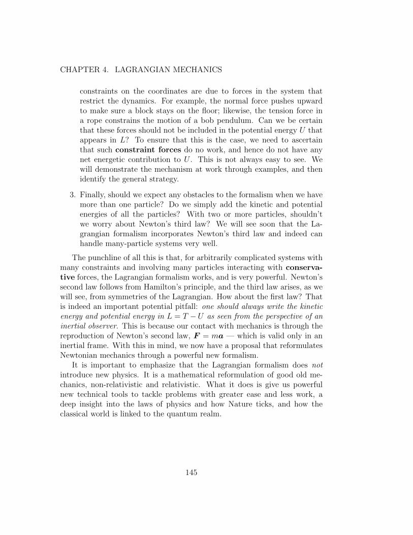
constraints on the coordinates are due to forces in the system thatrestrict the dynamics. For example, the normal force pushes upwardto make sure a block stays on the floor; likewise, the tension force ina rope constrains the motion of a bob pendulum. Can we be certainthat these forces should not be included in the potential energy U thatappears in L? To ensure that this is the case, we need to ascertainthat such constraint forces do no work, and hence do not have anynet energetic contribution to U . This is not always easy to see. Wewill demonstrate the mechanism at work through examples, and thenidentify the general strategy.

3. Finally, should we expect any obstacles to the formalism when we havemore than one particle? Do we simply add the kinetic and potentialenergies of all the particles? With two or more particles, shouldn’twe worry about Newton’s third law? We will see soon that the La-grangian formalism incorporates Newton’s third law and indeed canhandle many-particle systems very well.

The punchline of all this is that, for arbitrarily complicated systems withmany constraints and involving many particles interacting with conserva-tive forces, the Lagrangian formalism works, and is very powerful. Newton’ssecond law follows from Hamilton’s principle, and the third law arises, as wewill see, from symmetries of the Lagrangian. How about the first law? Thatis indeed an important potential pitfall: one should always write the kineticenergy and potential energy in L = T −U as seen from the perspective of aninertial observer. This is because our contact with mechanics is through thereproduction of Newton’s second law, F = ma — which is valid only in aninertial frame. With this in mind, we now have a proposal that reformulatesNewtonian mechanics through a powerful new formalism.

It is important to emphasize that the Lagrangian formalism does notintroduce new physics. It is a mathematical reformulation of good old me-chanics, non-relativistic and relativistic. What it does is give us powerfulnew technical tools to tackle problems with greater ease and less work, adeep insight into the laws of physics and how Nature ticks, and how theclassical world is linked to the quantum realm.

145


EXAMPLE 4-1: A simple pendulum

A small plumb bob of mass m is free to swing back and forth in a vertical x-z plane atthe end of a string of length R. The position of the bob can be specified uniquely by its angleθ measured up from its equilibrium position at the bottom, so we choose θ as the generalizedcoordinate. The bob’s kinetic energy is

T =1

2mv2 =

1

2m (x2 + z2) =

1

2m (r2 + r2θ2) =

1

2m (R2θ2) . (4.15)

Here, we switched to polar coordinates, and implemented the constraint equations r = 0 andr = R. Its potential energy is U = mgh = mgR(1− cos θ), measuring the bob’s height h upfrom its lowest point. The Lagrangian of the bob is therefore

L = T − U =1

2mR2θ2 −mgR(1− cos θ). (4.16)

The constraint reduces the dynamics from two planar coordinates to only one, the single degreeof freedom that is the angle θ. The single Euler equation in this case is

∂L

∂θ− d

dt

∂L

∂θ= −mgR sin θ − d

dt

(mR2θ

)= 0, (4.17)

equivalent to the well-known “pendulum equation”

θ + (g/R) sin θ = 0. (4.18)

Note that equation (4.17)) (or (4.18)) is equivalent to τ = Iθ, where the torque τ =−mgR sin θ is taken about the point of suspension (negative because it is opposite to thedirection of increasing θ), and the moment of inertia of the bob is I = mR2.

We had two twists in this problem. First, we switched from Cartesian to polar coordinates.But we know that this is not a problem for the Lagrangian formalism since the action is ascalar quantity. Second, we implemented a constraint r = R, implying r = 0. This constraintis responsible for holding the bob at fixed distance from the pivot and hence is due to thetension force in the rope. By implementing the constraint, we reduced the problem fromtwo to only one degree of freedom. Furthermore, the tension in the rope does no work: it isalways perpendicular to the motion of the bob, and hence the work contribution T · dr = 0,where T is the tension force and dr is the displacement of the bob. Thus, our potential energyU — related to work done by a force — was simply the potential energy due to gravity alone,U = mgh. In general, whenever a contact force is always perpendicular to the displacementof the particle it is acting on, it can safely be ignored in constructing the Lagrangian.

146


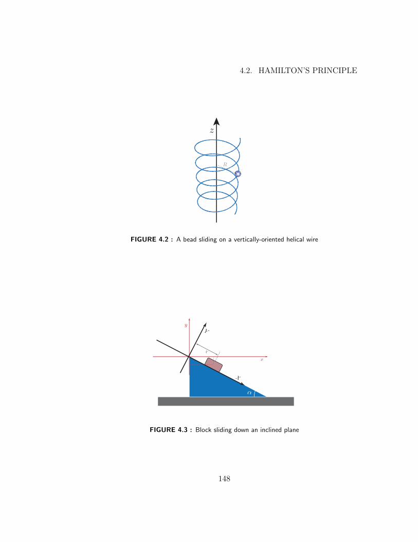
EXAMPLE 4-2: A bead sliding on a vertical helix

A bead of mass m is slipped onto a frictionless wire wound in the shape of a helix ofradius R, whose symmetry axis is oriented vertically in a uniform gravitational field, as shown inFigure 4.2. Using cylindrical coordinates r, θ, z, the base of the helix is located at z = 0, θ = 0,and the angle θ is related to the height z at any point by θ = αz, where α is a constant withdimensions of inverse length. The gravitational potential energy of the bead is U = mgz,and its kinetic energy is T = (1/2)mv2 = (1/2)m[r2 + r2θ2 + z2]. However, the constraintthat the bead slide along the helix tells us that the bead’s radius is constant at r = R, and(choosing z as the single generalized coordinate), θ = αz. Therefore the kinetic energy of thebead is simply

T =1

2mv2 =

1

2m (x2 + y2 + z2) =

1

2m (r2 + r2θ2 + z2)

= (1/2)m[0 + α2R2 + 1]z2 , (4.19)

where we switched to cylindrical coordinates and implemented the two constraints θ = αz andr = R. So the Lagrangian of the bead is

L = T − U =1

2m[1 + α2R2]z2 −mgz (4.20)

in terms of the single generalized coordinate z and its generalized velocity z. Two constraintsreduced the dynamics from three to only one degree of freedom. Note that in Newtonianmechanics we often need to take into account the normal force of the wire on the bead as one ofthe forces in F = ma; however, the normal force appears nowhere in the Lagrangian, becauseit does no work on the bead in this case — it is always perpendicular to the displacementof the bead4. In general, whenever a normal force is perpendicular to the displacement of aparticle it is acting on, we can safely ignore it in setting up the Lagrangian.

EXAMPLE 4-3: Block on an inclined plane

A block of mass m slides down a frictionless plane tilted at angle α to the horizontal, asshown in Figure 4.3. The gravitational potential energy is mgh = mgX sinα, where X is thedistance of the block up along the plane from its lowest point. Using X as the generalizedcoordinate, the velocity is X, and the Lagrangian of the block is

4In this simple case with a single normal force, the simplification is not very obvious.However, in more complicated scenarios we shall see later, the advantages of dropping thenormal force from the Lagrangian — versus the Newtonian approach – will become moreapparent.

147


FIGURE 4.2 : A bead sliding on a vertically-oriented helical wire

FIGURE 4.3 : Block sliding down an inclined plane

148


L = T − U =1

2mv2 − U =

1

2mX2 −mgX sinα, (4.21)

which depends explicitly upon a single coordinate (X) and a single velocity (X). Our singledegree of freedom is then X. The Euler equation is

∂L

∂X− d

dt

∂L

∂X= −mg sinα− d

dtmX = 0, or −mg sinα = mX, (4.22)

which is indeed the correct F = ma equation for the block along the tilted plane.

In this problem, we judiciously chose our only degree of freedom as X, the distance along

the inclined plane. We can think of this as a coordinate transformation from x,y as shown in

the Figure, to X,Y . We then have a constraint Y = 0, since the block cannot tunnel into

the plane. We are then left with a single degree of freedom, X. This constraint is associated

with the normal force. Furthermore, the normal force in this problem is always perpendicular

to the displacement of the block and thus does no work. Once again, the Lagrangian formal-

ism demonstrates its elegance and power by dropping from the computation a force – and a

corresponding equation – and reducing the effective number of degrees of freedom.

4.3 Generalized momenta and cyclic coordi-

nates

In Cartesian coordinates the kinetic energy of a particle is T = (1/2)m(x2 +y2 + z2), whose derivatives with respect to the velocity components are∂L/∂x = mx, etc., which are the components of momentum. So with gener-alized coordinates qk, it is natural to define the generalized momenta pkas

pk ≡∂L

∂qk. (4.23)

In terms of pk, the Lagrange equations become simply

dpkdt

=∂L

∂qk. (4.24)

Now sometimes a particular coordinate ql is absent from the Lagrangian. Itsgeneralized velocity ql is present, but not ql itself. A missing coordinate issaid to be a cyclic coordinate or an ignorable coordinate.5 For any

5Neither “cyclic” nor “ignorable” is a particularly appropriate or descriptive name for acoordinate absent from the Lagrangian, but they are nevertheless the conventional terms.In this book we will most often call any missing coordinate “cyclic”.

149

4.3. GENERALIZED MOMENTA AND CYCLIC COORDINATES

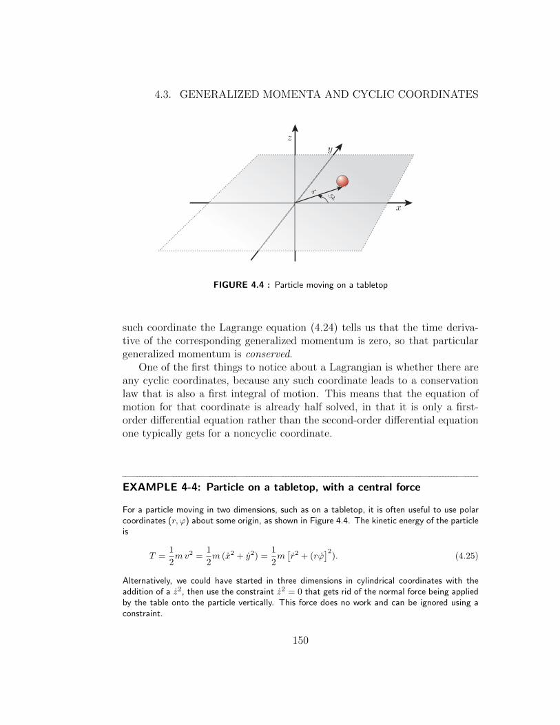
FIGURE 4.4 : Particle moving on a tabletop

such coordinate the Lagrange equation (4.24) tells us that the time deriva-tive of the corresponding generalized momentum is zero, so that particulargeneralized momentum is conserved.

One of the first things to notice about a Lagrangian is whether there areany cyclic coordinates, because any such coordinate leads to a conservationlaw that is also a first integral of motion. This means that the equation ofmotion for that coordinate is already half solved, in that it is only a first-order differential equation rather than the second-order differential equationone typically gets for a noncyclic coordinate.

EXAMPLE 4-4: Particle on a tabletop, with a central force

For a particle moving in two dimensions, such as on a tabletop, it is often useful to use polarcoordinates (r, ϕ) about some origin, as shown in Figure 4.4. The kinetic energy of the particleis

T =1

2mv2 =

1

2m (x2 + y2) =

1

2m[r2 + (rϕ

]2). (4.25)

Alternatively, we could have started in three dimensions in cylindrical coordinates with theaddition of a z2, then use the constraint z2 = 0 that gets rid of the normal force being appliedby the table onto the particle vertically. This force does no work and can be ignored using aconstraint.

150


We will assume here that any force acting on the particle is a central force, depending upon ralone, so the potential energy U of the particle also depends upon r alone. The Lagrangian istherefore

L =1

2m(r2 + r2ϕ2)− U(r). (4.26)

Our two degrees of freedom are r and ϕ. We note right away that in this case the coordinateϕ is cyclic, so there must be a conserved quantity

pϕ ≡∂L

∂ϕ= mr2ϕ, (4.27)

which we recognize as the angular momentum of the particle. In Lagrange’s approach,pϕ is conserved because ϕ is a cyclic coordinate; in Newtonian mechanics, pϕ is conservedbecause there is no torque on the particle, since we assumed that any force is a central force.The various partial derivatives of L are

∂L

∂r= mr

∂L

∂ϕ= mr2ϕ (4.28)

∂L

∂r= mrϕ2 − ∂U(r, ϕ)

∂r

∂L

∂ϕ= 0, (4.29)

so the Lagrange equations

∂L

∂r− d

dt

∂L

∂r= 0 and

∂L

∂ϕ− d

dt

∂L

∂ϕ= 0 (4.30)

become

mrϕ2 − ∂U(r)

∂r−mr = 0 and −mrϕ− 2mrϕ = 0 (4.31)

or (equivalently)

Fr = m(r − rϕ2) ≡ mar and Fϕ = m(rϕ+ 2rϕ) = 0, (4.32)

where the radial force is Fr = −∂U/∂r and the radial and tangential accelerations are

ar = r − rϕ2 and aϕ = rϕ+ 2rϕ, (4.33)

and where the tangential acceleration aϕ is zero in this case.6

In an example of Chapter 1 we found (using F = ma) the equations of motion of a particleof mass m on the end of a spring of zero natural length and force constant k, where one end

6Note how easy it is to get the expressions for radial and tangential accelerations inpolar coordinates using this method. They are often found in classical mechanics bydifferentiating the position vector r = rr twice with respect to time, which involves rathertricky derivatives of the unit vectors r and θ.

151


of the spring was fixed and the particle was free to move in two dimensions, as on a tabletop.There we used Cartesian coordinates (x, y). Now we are equipped to write the equations ofmotion in polar coordinates instead. Equations (4.30) with Fr = −kr and Fϕ = 0 give

−kr = m(r − rϕ2) and pϕ = mr2ϕ = constant. (4.34)

That is, since the Lagrangian is independent of ϕ, we get the immediate first integral of motionpϕ = constant. Eliminating ϕ between the two equations, we find the purely radial equation

r − (pϕ)2

m2r3+ ω2

0r = 0 (4.35)

where ω0 =√k/m is the natural frequency the spring-mass system would have if the mass were

oscillating in one dimension (which in fact it would do if the angular momentum pϕ happenedto be zero.) Note that even though the motion is generally two-dimensional, equation (4.35))contains only r(t); we can therefore find a first integral of this equation because it has theform of a one-dimensional F = ma equation with F = mr = (p2

ϕ/mr3 −mω2

0r. An effectiveone-dimensional potential energy can be found by setting F (r) = −dUeff(r)/dr; that is,

Ueff(r) = −∫ r

F (r) dr = −∫ r ( (pϕ)2

mr3−mω2

0r

)dr =

(pϕ)2

2mr2+

1

2kr2 (4.36)

plus a constant of integration, which we might as well set to zero. Therefore, a first integralof motion is

1

2mr2 +

(pϕ)2

2mr2+

1

2kr2 =

1

2mr2 + Ueff = constant. (4.37)

A sketch of Ueff is shown in Figure 4.5. Note that Ueff has a minimum, which is the loca-

tion of an equilibrium point (the value of r for which dUeff(r)/dr = 0 is of course also the

radius for which r = 0.) If r remains at the minimum of Ueff , the mass is actually circling

the origin. The motion about this point is stable because the potential energy is a minimum

there. For small displacements from equilibrium the particle oscillates back and forth about

this equilibrium radius as it orbits the origin. In Section 4.7 we will calculate the frequency

of these oscillations. This example demonstrates the use of coordinate transformations in

the Lagrangian formalism. We already knew the formalism goes through under a coordinate

change. In this case, we see how useful it can be to use this freedom at the Lagrangian level.

EXAMPLE 4-5: The spherical pendulum

152


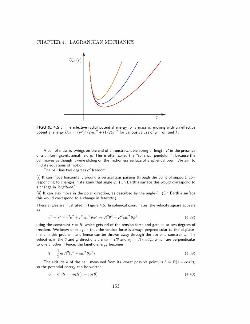
FIGURE 4.5 : The effective radial potential energy for a mass m moving with an effectivepotential energy Ueff = (pϕ)2/2mr2 + (1/2)kr2 for various values of pϕ, m, and k.

A ball of mass m swings on the end of an unstretchable string of length R in the presenceof a uniform gravitational field g. This is often called the “spherical pendulum”, because theball moves as though it were sliding on the frictionless surface of a spherical bowl. We aim tofind its equations of motion.

The ball has two degrees of freedom:

(i) It can move horizontally around a vertical axis passing through the point of support, cor-responding to changes in its azimuthal angle ϕ. (On Earth’s surface this would correspond toa change in longitude.)

(ii) It can also move in the polar direction, as described by the angle θ. (On Earth’s surfacethis would correspond to a change in latitude.)

These angles are illustrated in Figure 4.6. In spherical coordinates, the velocity square appearsas

v2 = r2 + r2θ2 + r2 sin2 θϕ2 ⇒ R2θ2 +R2 sin2 θϕ2 (4.38)

using the constraint r = R, which gets rid of the tension force and gets us to two degrees offreedom. We know once again that the tension force is always perpendicular to the displace-ment in this problem, and hence can be thrown away through the use of a constraint. Thevelocities in the θ and ϕ directions are vθ = Rθ and vϕ = R sin θϕ, which are perpendicularto one another. Hence, the kinetic energy becomes

T =1

2mR2(θ2 + sin2 θϕ2) (4.39)

The altitude h of the ball, measured from its lowest possible point, is h = R(1 − cos θ),so the potential energy can be written

U = mgh = mgR(1− cos θ). (4.40)

153


FIGURE 4.6 : Coordinates of a ball hanging on an unstretchable string

The Lagrangian is therefore

L = T − U =1

2mR2(θ2 + sin2 θϕ2)−mgR(1− cos θ) . (4.41)

Our two degrees of freedom are then θ and ϕ. The derivatives are

∂L

∂θ= mR2 sin θ cos θϕ2 −mgR sin θ

∂L

∂θ= mR2θ (4.42)

∂L

∂ϕ= 0

∂L

∂ϕ= mR2 sin2 θ ϕ. (4.43)

The Lagrange equations become

∂L

∂θ− d

dt

∂L

∂θ= 0 and

∂L

∂ϕ− d

dt

∂L

∂ϕ= 0, (4.44)

but before writing them out, note that ϕ is cyclic, so the corresponding generalized momentumis

pϕ =∂L

∂ϕ= mR2 sin2 θ ϕ = constant, (4.45)

which is an immediate first integral of motion. (We identify pϕ as the angular momentumabout the vertical axis.)

Now since

d

dt

(mR2θ

)= mR2θ, (4.46)

154


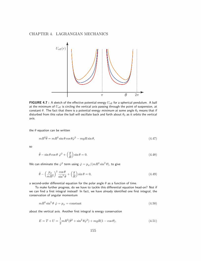
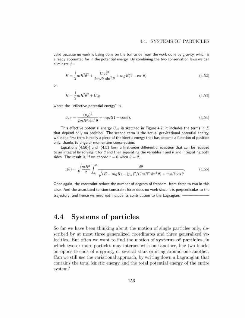
FIGURE 4.7 : A sketch of the effective potential energy Ueff for a spherical pendulum. A ballat the minimum of Ueff is circling the vertical axis passing through the point of suspension, atconstant θ. The fact that there is a potential energy minimum at some angle θ0 means that ifdisturbed from this value the ball will oscillate back and forth about θ0 as it orbits the verticalaxis.

the θ equation can be written

mR2θ = mR2 sin θ cos θϕ2 −mgR sin θ, (4.47)

so

θ − sin θ cos θ ϕ2 +( gR

)sin θ = 0. (4.48)

We can eliminate the ϕ2 term using ϕ = pϕ/(mR2 sin2 θ), to give

θ −( pϕmR2

)2 cos θ

sin3 θ+( gR

)sin θ = 0, (4.49)

a second-order differential equation for the polar angle θ as a function of time.To make further progress, do we have to tackle this differential equation head-on? Not if

we can find a first integral instead! In fact, we have already identified one first integral, theconservation of angular momentum

mR2 sin2 θ ϕ = pϕ = constant (4.50)

about the vertical axis. Another first integral is energy conservation

E = T + U =1

2mR2(θ2 + sin2 θϕ2) +mgR(1− cos θ), (4.51)

155

4.4. SYSTEMS OF PARTICLES

valid because no work is being done on the ball aside from the work done by gravity, which isalready accounted for in the potential energy. By combining the two conservation laws we caneliminate ϕ:

E =1

2mR2θ2 +

(pϕ)2

2mR2 sin2 θ+mgR(1− cos θ) (4.52)

or

E =1

2mR2θ2 + Ueff (4.53)

where the “effective potential energy” is

Ueff =(pϕ)2

2mR2 sin2 θ+mgR(1− cos θ). (4.54)

This effective potential energy Ueff is sketched in Figure 4.7; it includes the terms in Ethat depend only on position. The second term is the actual gravitational potential energy,while the first term is really a piece of the kinetic energy that has become a function of positiononly, thanks to angular momentum conservation.

Equations (4.50)) and (4.51 form a first-order differential equation that can be reducedto an integral by solving it for θ and then separating the variables t and θ and integrating bothsides. The result is, if we choose t = 0 when θ = θ0,

t(θ) =

√mR2

2

∫ θ

θ0

dθ√(E −mgR)− (pϕ)2/(2mR2 sin2 θ) +mgR cos θ

. (4.55)

Once again, the constraint reduce the number of degrees of freedom, from three to two in this

case. And the associated tension constraint force does no work since it is perpendicular to the

trajectory; and hence we need not include its contribution to the Lagragian.

4.4 Systems of particles

So far we have been thinking about the motion of single particles only, de-scribed by at most three generalized coordinates and three generalized ve-locities. But often we want to find the motion of systems of particles, inwhich two or more particles may interact with one another, like two blockson opposite ends of a spring, or several stars orbiting around one another.Can we still use the variational approach, by writing down a Lagrangian thatcontains the total kinetic energy and the total potential energy of the entiresystem?

156


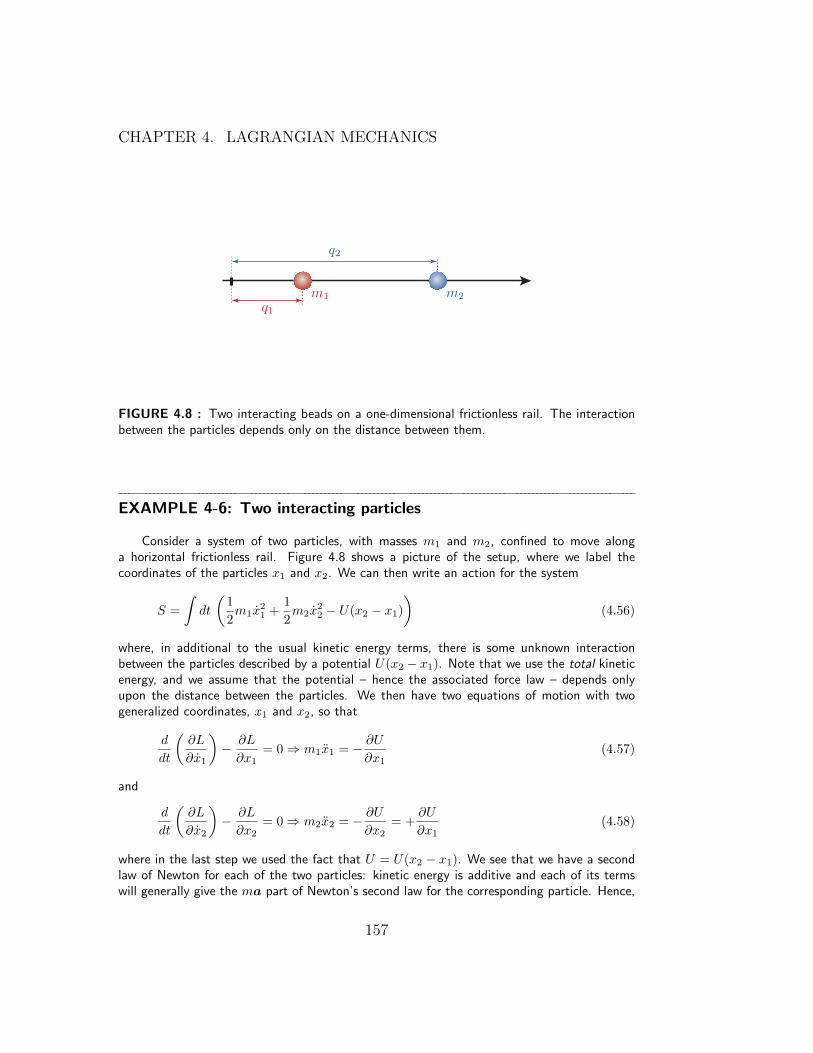
FIGURE 4.8 : Two interacting beads on a one-dimensional frictionless rail. The interactionbetween the particles depends only on the distance between them.

EXAMPLE 4-6: Two interacting particles

Consider a system of two particles, with masses m1 and m2, confined to move alonga horizontal frictionless rail. Figure 4.8 shows a picture of the setup, where we label thecoordinates of the particles x1 and x2. We can then write an action for the system

S =

∫dt

(1

2m1x

21 +

1

2m2x

22 − U(x2 − x1)

)(4.56)

where, in additional to the usual kinetic energy terms, there is some unknown interactionbetween the particles described by a potential U(x2 − x1). Note that we use the total kineticenergy, and we assume that the potential – hence the associated force law – depends onlyupon the distance between the particles. We then have two equations of motion with twogeneralized coordinates, x1 and x2, so that

d

dt

(∂L

∂x1

)− ∂L

∂x1= 0⇒ m1x1 = − ∂U

∂x1(4.57)

and

d

dt

(∂L

∂x2

)− ∂L

∂x2= 0⇒ m2x2 = − ∂U

∂x2= +

∂U

∂x1(4.58)

where in the last step we used the fact that U = U(x2 − x1). We see that we have a secondlaw of Newton for each of the two particles: kinetic energy is additive and each of its termswill generally give the ma part of Newton’s second law for the corresponding particle. Hence,

157


in multi-particle systems, we need to consider the total kinetic energy T minus the totalpotential energy. Terms that mix the variables of different particles, such as U(x2 − x1), willgive the correct forces on the particles as well. In this case, we see that the action-reactionpair, ∂U/∂x1 = −∂U/∂x2, comes out for free, and arises from the fact that the force lawdepends only on the distance between the particles! That is, Newton’s third law is naturallyincorporated in the formalism and originates from the fact that forces between two particlesdepend only upon the distance between the interacting entities, and not (say) their absolutepositions.

Suppose for example that the particles are connected by a Hooke’s-law spring of forceconstant k. If we choose the coordinates x1 and x2 appropriately, the spring stretch will bex2 − x1, so the potential energy is U = (1/2)k(x2 − x1)2. The Lagrange equations then give

m1x1 = +k(x2 − x1) and m2x2 = −k(x2 − x1). (4.59)

The forces on the two particles are obviously equal but opposite: In such a case the totalmomentum of the systems must be conserved, which is easily verified simply by adding thetwo equations, to show that

d

dt(m1x1 +m2x2) = 0. (4.60)

There are actually two conserved quantities in this problem, the momentum and the energy,each of which leads to a first integral of motion.

These results suggest that there must be a more transparent set of generalized coordinatesto use here, in which one of the new coordinates is cyclic, so that its generalized momentumwill be conserved automatically. These new coordinates are the center of mass and relativecoordinates

X ≡ m1x1 +m2x2

Mand x ≡ x2 − x1, (4.61)

where M = m1 + m2 is the total mass of the system: Note that X and x are simply linearcombinations of x1 and x2. Then in terms of X and x, it is straightforward to show that theLagrangian of the system becomes

L =1

2MX2 +

1

2µx2 − U(x) (4.62)

where µ ≡ m1m2/M is called the reduced mass of the system (note that µ is in fact smallerthan either m1 or m2.) Using this Lagrangian, it is obvious that the center of mass coordinateX is cyclic, so the corresponding momentum

P =∂L

∂X= MX ≡ m1x1 +m2x2 (4.63)

is conserved (as we saw before).This problem is an example of reducing a two-body problem to an equivalent one-body

problem through a coordinate transformation. The motion of the center of mass of the systemis trivial: the center of mass just drifts along at constant velocity. The interesting motion of

158


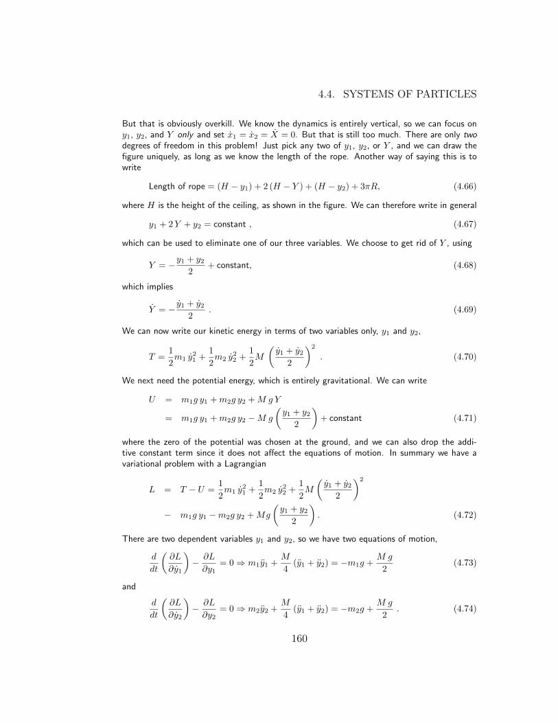
FIGURE 4.9 : A contraption of pulleys. We want to find the accelerations of all three weights.We assume that the pulleys have negligible mass so they have negligible kinetic and potentialenergies.

the particles is their relative motion x, which behaves as though it were a single particle ofmass µ and position x(t) subject to the potential energy U(x) with Lagrangian

L =1

2µx2 − U(x) . (4.64)

Hence, coordinate transforming at the Lagrangian level can be very powerful technique.

EXAMPLE 4-7: Pulleys everywhere

Another classic set of mechanics problems involves pulleys, lots of pulleys. Consider thesetup shown in Figure 4.9. Two weights, with masses m1 and m2, hang on the outside ofa three-pulley system, while a weight of mass M hangs on the middle pulley. We assume thepulleys and the connecting rope have negligible mass, so their kinetic and potential energiesare also negligible. We will suppose for now that all three pulleys have the same radius R, butthis will turn out to be of no importance. We want to find the accelerations of m1, m2, andM . We construct a Cartesian coordinate system as shown in the figure, which is at rest in aninertial frame of the ground. First of all, note that there are three massive objects moving intwo dimensions, so we might think that we have six variables to track, x1 and y1 for weightm1, x2 and y2 for weight m2, and X and Y for weight M . We can then write the total kineticenergy

T =1

2m1 (x2

1 + y21) +

1

2m2 (x2

2 + y22) +

1

2M (X2 + Y 2). (4.65)

159


But that is obviously overkill. We know the dynamics is entirely vertical, so we can focus ony1, y2, and Y only and set x1 = x2 = X = 0. But that is still too much. There are only twodegrees of freedom in this problem! Just pick any two of y1, y2, or Y , and we can draw thefigure uniquely, as long as we know the length of the rope. Another way of saying this is towrite

Length of rope = (H − y1) + 2 (H − Y ) + (H − y2) + 3πR, (4.66)

where H is the height of the ceiling, as shown in the figure. We can therefore write in general

y1 + 2Y + y2 = constant , (4.67)

which can be used to eliminate one of our three variables. We choose to get rid of Y , using

Y = −y1 + y2

2+ constant, (4.68)

which implies

Y = − y1 + y2

2. (4.69)

We can now write our kinetic energy in terms of two variables only, y1 and y2,

T =1

2m1 y

21 +

1

2m2 y

22 +

1

2M

(y1 + y2

2

)2

. (4.70)

We next need the potential energy, which is entirely gravitational. We can write

U = m1g y1 +m2g y2 +M g Y

= m1g y1 +m2g y2 −M g

(y1 + y2

2

)+ constant (4.71)

where the zero of the potential was chosen at the ground, and we can also drop the addi-tive constant term since it does not affect the equations of motion. In summary we have avariational problem with a Lagrangian

L = T − U =1

2m1 y

21 +

1

2m2 y

22 +

1

2M

(y1 + y2

2

)2

− m1g y1 −m2g y2 +Mg

(y1 + y2

2

). (4.72)

There are two dependent variables y1 and y2, so we have two equations of motion,

d

dt

(∂L

∂y1

)− ∂L

∂y1= 0⇒ m1y1 +

M

4(y1 + y2) = −m1g +

M g

2(4.73)

and

d

dt

(∂L

∂y2

)− ∂L

∂y2= 0⇒ m2y2 +

M

4(y1 + y2) = −m2g +

M g

2. (4.74)

160


We can now solve for y1 and y2,

y1 = −g +4m2g

m1 +m2 + 4m1m2/M

y2 = −g +4m1g

m1 +m2 + 4m1m2/M. (4.75)

Note that these accelerations have magnitudes less than g, as we might expect intuitively. Wecan also find Y from (4.69)

Y = − y1 + y2

2⇒ Y = g − 2 (m1 +m2)g

m1 +m2 + 4m1m2/M. (4.76)

The constraint given by (4.66), which eliminated one of our three original variables, imple-

ments the physical condition that the rope has constant length. This is related to the tension

force in the rope. The astute reader may rightfully wonder whether we have overlooked some-

thing in this treatment: we never encountered the tension force of the rope on each of the

masses! Consider the two tension forces T1 and T2 at the end of this (or any) massless rope. If

we wanted to account for such forces in a Lagrangian, we would need the associated energy, or

work they contribute to the system. Since the rope has zero mass, we know that |T1| = |T2|.The two tension forces however point in opposite directions. When one end of the rope moves

by ∆x1 > 0 parallel to T1, T1 does work W1 = |T1|∆x1. At the same time, the other end must

move the same distance ∆x2 = ∆x1. However, at this other end, the tension force points

opposite to the displacement, and the work is W2 = −|T2|∆x2 = −|T1|∆x1. The total work

is W = W1 +W2 = 0. Hence, the tension forces along a massless rope will always contribute

zero work, and hence cannot be associated with energy in the Lagrangian. Similarly, this is

the case for any force that appears in a problem in an action-reaction pair, as we shall see next.

EXAMPLE 4-8: A block on a movable inclined plane

Let us return to the classic problem of a block sliding down a frictionless inclined plane, asin Example 2, except we will make things a bit more interesting: now the inclined plane itselfis allowed to move! Figure 4.10(a) shows the setup. A block of mass m rests on an inclinedplane of mass M : Both the block and the inclined plane are free to move without friction.The plane’s angle is denoted by α. The problem is to find the acceleration of the block.

The observation deck is the ground, which is taken as an inertial reference frame. Weset up a convenient set of Cartesian coordinates, as shown in the figure. The origin is shiftedto the top of the incline at zero time to make the geometry easier to analyze. We start byidentifying the degrees of freedom. At first, we can think of the block and inclined plane as

161


(a) (b)

FIGURE 4.10 : A block slides along an inclined plane. Both block and inclined plane are freeto move along frictionless surfaces.

moving in the two dimensions of the problem. The block’s coordinates could be denoted byx and y, and the inclined plane’s coordinates by X and Y . But we quickly realize that thiswould be overkill: if we specify X, and how far down the top of the incline the block is located(denoted by D in the figure), we can draw the figure uniquely. This is because the inclinedplane cannot move vertically, either jumping off the ground or burrowing into it (that’s onecondition), so Y is unnecessary, and the horizontal position x of the block is determined by Xand D (that’s a second condition.) We then start with four coordinates, add two conditionsor restrictions, and we are left with two degrees of freedom. The choice of the two remainingdegrees of freedom is arbitrary, as long as the choice uniquely fixes the geometry. We will pickX and D; another choice might be X and x, for example.

Next, we need to write the Lagrangian. The starting point for this is the total kineticenergy of the system,

T =1

2m(x2 + y2

)+

1

2M(X2 + Y 2

)(4.77)

in the inertial frame of the ground. Note the importance of writing the kinetic energy in aninertial frame, even if it means using more coordinates than the generalized coordinates thatwill be used in the Lagrangian.

Now we need to rewrite the kinetic energy in terms of the two degrees of freedom X andD alone. This requires a little bit of geometry. Looking back at the figure, we can write

Y = 0 , x = X +D cosα , y = −D sinα . (4.78)

This implies

Y = 0 , x = X + D cosα , y = −D sinα . (4.79)

162


We can now substitute these into (4.77) and get

T =1

2M X2 +

1

2mX2 +

1

2mD2 +mX D cosα . (4.80)

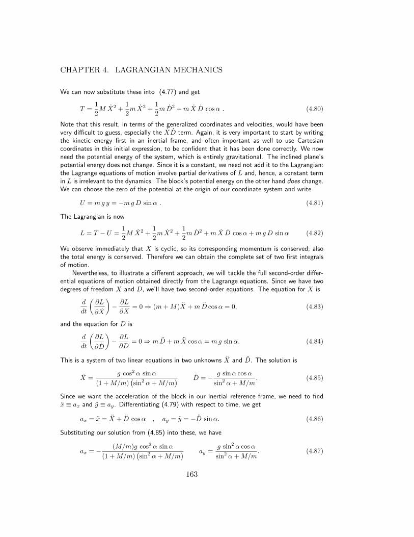
Note that this result, in terms of the generalized coordinates and velocities, would have beenvery difficult to guess, especially the XD term. Again, it is very important to start by writingthe kinetic energy first in an inertial frame, and often important as well to use Cartesiancoordinates in this initial expression, to be confident that it has been done correctly. We nowneed the potential energy of the system, which is entirely gravitational. The inclined plane’spotential energy does not change. Since it is a constant, we need not add it to the Lagrangian:the Lagrange equations of motion involve partial derivatives of L and, hence, a constant termin L is irrelevant to the dynamics. The block’s potential energy on the other hand does change.We can choose the zero of the potential at the origin of our coordinate system and write

U = mg y = −mgD sinα . (4.81)

The Lagrangian is now

L = T − U =1

2M X2 +

1

2mX2 +

1

2mD2 +mX D cosα+mgD sinα (4.82)

We observe immediately that X is cyclic, so its corresponding momentum is conserved; alsothe total energy is conserved. Therefore we can obtain the complete set of two first integralsof motion.

Nevertheless, to illustrate a different approach, we will tackle the full second-order differ-ential equations of motion obtained directly from the Lagrange equations. Since we have twodegrees of freedom X and D, we’ll have two second-order equations. The equation for X is

d

dt

(∂L

∂X

)− ∂L

∂X= 0⇒ (m+M)X +mD cosα = 0, (4.83)

and the equation for D is

d

dt

(∂L

∂D

)− ∂L

∂D= 0⇒ mD +mX cosα = mg sinα. (4.84)

This is a system of two linear equations in two unknowns X and D. The solution is

X =g cos2 α sinα

(1 +M/m)(sin2 α+M/m

) D = − g sinα cosα

sin2 α+M/m. (4.85)

Since we want the acceleration of the block in our inertial reference frame, we need to findx ≡ ax and y ≡ ay. Differentiating (4.79) with respect to time, we get

ax = x = X + D cosα , ay = y = −D sinα. (4.86)

Substituting our solution from (4.85) into these, we have

ax = − (M/m)g cos2 α sinα

(1 +M/m)(sin2 α+M/m

) ay =g sin2 α cosα

sin2 α+M/m. (4.87)

163

4.5. THE HAMILTONIAN

It is always useful to look at various limiting cases, to see if a result makes sense. For example,what if α = 0, i.e., what if the block moves on a horizontal plane? Both accelerations thenvanish, as expected: if started at rest, both block and incline just stay put. Now what if theinclined plane is much heavier than the block, with M m? We then have

ax ' −m

Mg cos2 α sinα ay '

m

Mg sin2 α cosα, (4.88)

so that ay/ax ' − tanα, which is what we would expect if the inclined plane were not movingappreciably.

The computational step at the beginning where we zeroed onto the degrees of freedomof the problem – going from X, Y , x, and y to X and D – is associated with the normalforces. The most impressive aspect of this example is the absence of any normal forces fromour computations! With the traditional approach of problem solving, we would need to includeseveral normal forces in the computation, shown in Figure 4.10(b): the normal force exerted bythe inclined plane on the block, the normal force exerted by the ground on the inclined plane,and the normal force exerted by the block on the inclined plane as a reaction force. The roleof these normal forces is to hold the inclined plane on the ground and to hold the block onthe inclined plane. If we think of the contributions of the normal forces to the Lagrangian, wewould want to include some potential energy terms for them. But potential energy is relatedto work done by forces. The normal force is often perpendicular to the direction of motion,and hence does no work, N ·∆r = 0. Hence, there is no potential energy term to include inthe Lagrangian to account for such normal forces. In our example, this is not entirely correct...While it is true for the normal force exerted by the ground onto the inclined plane, it is nottrue for the normal forces acting between the block and inclined plane. This is because theinclined plane is moving as well and the trajectory of the block is not parallel to the incline!However, there is another reason why this normal force is safely left out of the Lagrangianmethod. These normal forces occur as an action-reaction pair. And the displacement of theinterface between the block and incline is the same for both forces, and hence the contributionsto the total work or energy of the system from these two normal forces cancel. As we sawfrom the previous example, such forces do not appear in the Lagrangian.

In a later chapter we will also learn of a way to impose the inclusion of normal and ten-

sion forces in a Lagrangian even when we need not do so — for the purpose of finding the

magnitude of a normal force if it is desired. For now, we are very happy to drop normal and

tension forces from consideration. This can be a big simplification for problem solving: fewer

variables, fewer forces to consider, less work to do (no pun intended).

4.5 The Hamiltonian

We will now prove an enormously useful mathematical consequence of theLagrange equations, providing one more potential way to achieve a first in-tegral of motion, which we can add to the arsenal of approaches already

164


summarized in the preceding section. First, take the total derivative of theLagrangian L(t, qk, qk) with respect to time t. There are many ways in whichL can change: it can change because of explicit changes in t, and also becauseof implicit changes in t due to the time dependence of one or more of thecoordinates qk(t) or velocities qk(t). Therefore, from multivariable calculus,

dL(qk, qk, t)

dt=∂L

∂t+∂L

∂qkqk +

∂L

∂qkqk, (4.89)

using the Einstein summation convention from Chapter 2. That is, since theindex k is repeated in each of the last two terms, a sum over k is implied ineach term; we have also used the fact that dqk/dt ≡ qk. Now, take the timederivative of the quantity qk(∂L/∂qk); again, sums over k are implied:

d

dt

(qk∂L

∂qk

)= qk

∂L

∂qk+ qk

d

dt

(∂L

∂qk

)= qk

∂L

∂qk+ qk

∂L

∂qk(4.90)

using the product rule. We have also used the Lagrange equations to simplifythe second term on the right. Note that this expression contains the sametwo summed terms that we found in equation (4.89)). Therefore, subtractingequation (4.90) from equation (4.89 gives

∂L

∂t− d

dt

(L− qk

∂L

∂qk

)= 0. (4.91)

This result is particularly interesting if L is not an explicit function of time,i.e., , if ∂L/∂t = 0. In fact, define the Hamiltonian H of a particle to be

H ≡ qk pk − L (4.92)

where we have already defined the generalized momenta to be pi = ∂L/∂qk,and again a sum over k is implied. Then equation (4.91) can be written

∂L

∂t= −dH

dt, (4.93)

an extremely useful result! It shows that if a Lagrangian L is not an explicitfunction of time, then the Hamiltonian H is conserved.

What is the meaning of H? Suppose that our particle is free to movein three dimensions in a potential U(x, y, z) without constraints, and that

165


we are using Cartesian coordinates. Then px = mx, etc., so∑

i qkpk =m(x2 + y2 + z2). Therefore,

H = m(x2 + y2 + z2)− 1

2m(x2 + y2 + z2) + U(x, y, z)

=1

2m(x2 + y2 + z2) + U(x, y, z) = T + U = E, (4.94)

which is simply the energy of the particle!Is H always equal to E = T + U? The answer is no, although very often

it is. The precise conditions for which H 6= E are derived in Appendix A.

EXAMPLE 4-9: Bead on a rotating parabolic wire

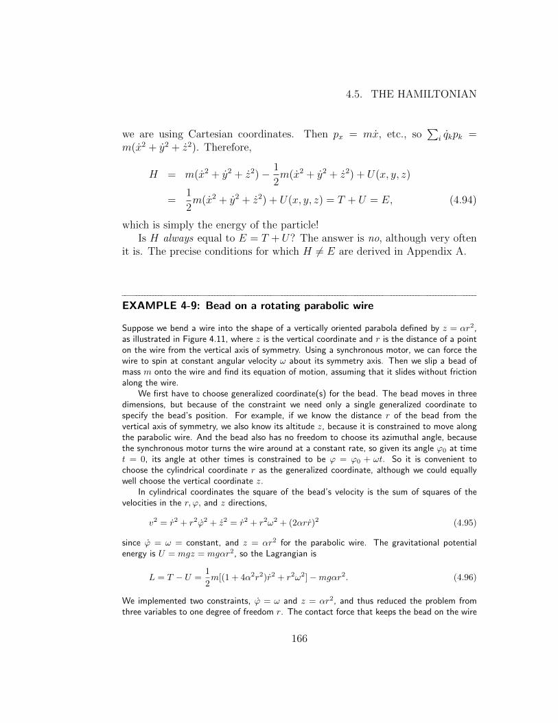
Suppose we bend a wire into the shape of a vertically oriented parabola defined by z = αr2,as illustrated in Figure 4.11, where z is the vertical coordinate and r is the distance of a pointon the wire from the vertical axis of symmetry. Using a synchronous motor, we can force thewire to spin at constant angular velocity ω about its symmetry axis. Then we slip a bead ofmass m onto the wire and find its equation of motion, assuming that it slides without frictionalong the wire.

We first have to choose generalized coordinate(s) for the bead. The bead moves in threedimensions, but because of the constraint we need only a single generalized coordinate tospecify the bead’s position. For example, if we know the distance r of the bead from thevertical axis of symmetry, we also know its altitude z, because it is constrained to move alongthe parabolic wire. And the bead also has no freedom to choose its azimuthal angle, becausethe synchronous motor turns the wire around at a constant rate, so given its angle ϕ0 at timet = 0, its angle at other times is constrained to be ϕ = ϕ0 + ωt. So it is convenient tochoose the cylindrical coordinate r as the generalized coordinate, although we could equallywell choose the vertical coordinate z.

In cylindrical coordinates the square of the bead’s velocity is the sum of squares of thevelocities in the r, ϕ, and z directions,

v2 = r2 + r2ϕ2 + z2 = r2 + r2ω2 + (2αrr)2 (4.95)

since ϕ = ω = constant, and z = αr2 for the parabolic wire. The gravitational potentialenergy is U = mgz = mgαr2, so the Lagrangian is

L = T − U =1

2m[(1 + 4α2r2)r2 + r2ω2]−mgαr2. (4.96)

We implemented two constraints, ϕ = ω and z = αr2, and thus reduced the problem fromthree variables to one degree of freedom r. The contact force that keeps the bead on the wire

166


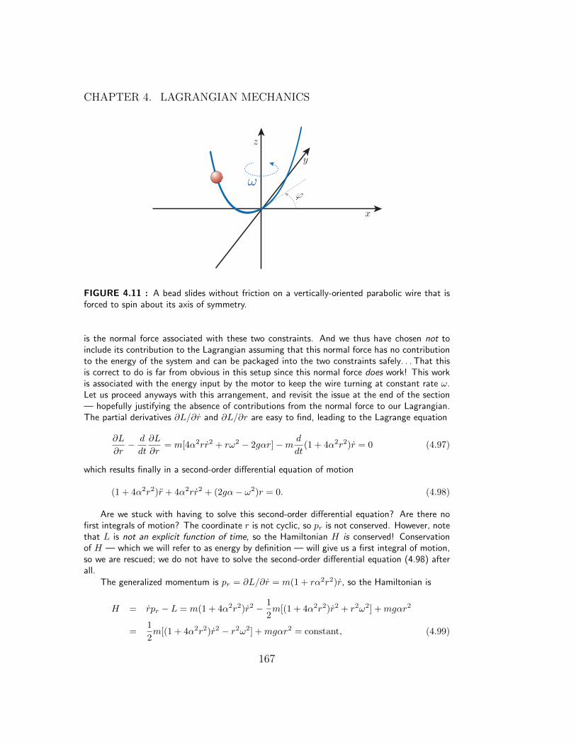
FIGURE 4.11 : A bead slides without friction on a vertically-oriented parabolic wire that isforced to spin about its axis of symmetry.

is the normal force associated with these two constraints. And we thus have chosen not toinclude its contribution to the Lagrangian assuming that this normal force has no contributionto the energy of the system and can be packaged into the two constraints safely. . . That thisis correct to do is far from obvious in this setup since this normal force does work! This workis associated with the energy input by the motor to keep the wire turning at constant rate ω.Let us proceed anyways with this arrangement, and revisit the issue at the end of the section— hopefully justifying the absence of contributions from the normal force to our Lagrangian.The partial derivatives ∂L/∂r and ∂L/∂r are easy to find, leading to the Lagrange equation

∂L

∂r− d

dt

∂L

∂r= m[4α2rr2 + rω2 − 2gαr]−m d

dt(1 + 4α2r2)r = 0 (4.97)

which results finally in a second-order differential equation of motion

(1 + 4α2r2)r + 4α2rr2 + (2gα− ω2)r = 0. (4.98)

Are we stuck with having to solve this second-order differential equation? Are there nofirst integrals of motion? The coordinate r is not cyclic, so pr is not conserved. However, notethat L is not an explicit function of time, so the Hamiltonian H is conserved! Conservationof H — which we will refer to as energy by definition — will give us a first integral of motion,so we are rescued; we do not have to solve the second-order differential equation (4.98) afterall.

The generalized momentum is pr = ∂L/∂r = m(1 + rα2r2)r, so the Hamiltonian is

H = rpr − L = m(1 + 4α2r2)r2 − 1

2m[(1 + 4α2r2)r2 + r2ω2] +mgαr2

=1

2m[(1 + 4α2r2)r2 − r2ω2] +mgαr2 = constant, (4.99)

167


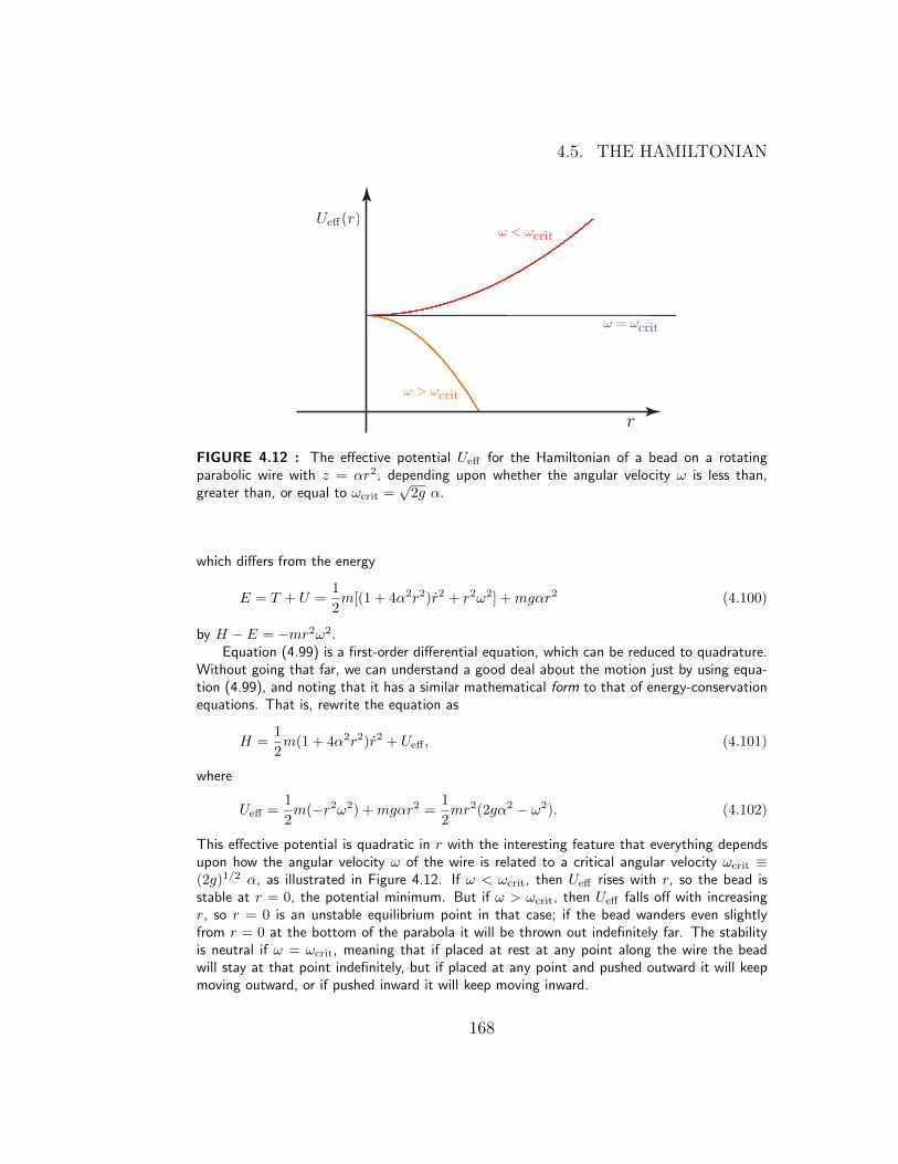
FIGURE 4.12 : The effective potential Ueff for the Hamiltonian of a bead on a rotatingparabolic wire with z = αr2, depending upon whether the angular velocity ω is less than,greater than, or equal to ωcrit =

√2g α.

which differs from the energy

E = T + U =1

2m[(1 + 4α2r2)r2 + r2ω2] +mgαr2 (4.100)

by H − E = −mr2ω2.Equation (4.99) is a first-order differential equation, which can be reduced to quadrature.

Without going that far, we can understand a good deal about the motion just by using equa-tion (4.99), and noting that it has a similar mathematical form to that of energy-conservationequations. That is, rewrite the equation as

H =1

2m(1 + 4α2r2)r2 + Ueff , (4.101)

where

Ueff =1

2m(−r2ω2) +mgαr2 =

1

2mr2(2gα2 − ω2). (4.102)

This effective potential is quadratic in r with the interesting feature that everything dependsupon how the angular velocity ω of the wire is related to a critical angular velocity ωcrit ≡(2g)1/2 α, as illustrated in Figure 4.12. If ω < ωcrit, then Ueff rises with r, so the bead isstable at r = 0, the potential minimum. But if ω > ωcrit, then Ueff falls off with increasingr, so r = 0 is an unstable equilibrium point in that case; if the bead wanders even slightlyfrom r = 0 at the bottom of the parabola it will be thrown out indefinitely far. The stabilityis neutral if ω = ωcrit, meaning that if placed at rest at any point along the wire the beadwill stay at that point indefinitely, but if placed at any point and pushed outward it will keepmoving outward, or if pushed inward it will keep moving inward.

168


This example shows that although the Hamiltonian function H is often equal to E ≡ T+U ,this is not always so. Appendix A at the end of the chapter explains when and why they candiffer. In any case, the Hamiltonian can be very useful, because it provides a first integral ofmotion if L is not explicitly time-dependent. It is also the starting point for an alternativeapproach to classical dynamics, as we will see in a later chapter, and it turns out to be animportant bridge between classical and quantum mechanics7.

Let us come back to the issue of dropping the normal force’s contribution to our La-grangian. Since the bead is sliding along the wire while rotating with it, and since the normalforce is some vector perpendicular to the wire at any instant in time, we can see that thisnormal force is not necessarily perpendicular to the bead’s displacement. Hence, it can havenon-zero contribution to the energy of the system. This is why E is not conserved in theproblem; the conserved quantity is H which is not equal to E in this case. Nevertheless, howcan we justify dropping the normal force that we know can do work and hence may perhapshave a piece of U in L = T − U?

The answer is a delicate one: in constructing a Lagrangian, we need to include all objectsthat are moving around. The full system is bead plus rotating parabolic wire. The parabolicwire is not a free dynamical object since its motion is prescribed externally through the actionof the motor. You can think of such a non-dynamical object as one with zero mass; i.e., , ithas no contribution to the kinetic energy of the system. In reality, it has a constant non-zerocontribution, but a constant term in a Lagrangian does not effect the equations of motion.Hence, for simplicity, we can drop such a term altogether. However, forces can still act on itand do work. In this case, there is a normal force — equal but opposite in direction to the oneacting on the bead — acting on the wire. The point of action of this normal on the wire isdisplaced by the same amount as the bead. Hence, the contribution to the work of the systemof this normal force is equal in magnitude but opposite in sign to the contribution coming fromthe normal force acting on the bead. This is simply a reflection of Newton’s third law: forevery action, there is an equal but opposite reaction. The net contribution to work from thesetwo normal forces adds up to zero. Hence, when we write U for the system, we only need toconsider the contribution from gravity! We have L = T −U as before, without a trace of thenormal forces.

Once again, the Lagrangian formalism avoids dealing with contact forces and accounts for

them through constraints – simplifying the problem significantly. We leave it as an exercise

for the reader to solve this same problem using traditional force body diagram methods so as

to appreciate the power of the Lagrangian formalism.

7In a different approach we will see in Chapter 6, conserved quantities are definedthrough associated symmetries in Nature. Within such a convention, the Hamiltonianwould be defined as energy, and the combination T + U loses its privileged name andplace.

169

4.6. THE MORAL OF CONSTRAINTS

4.6 The moral of constraints

Let us summarize the steps we have used so far in setting up and preparingto solve Lagrange’s equations.

1. We identify the degrees of freedom of each particle or object consis-tent with any constraints, and choose an appropriate set of generalizedcoordinates qk for each.

2. Write the square of the velocity for each particle in terms of any conve-nient coordinates, usually Cartesian coordinates, in some inertial ref-erence frame. Then reexpress the kinetic energy in terms of the gen-eralized coordinates qk, the generalized velocities qk, and the time ifneeded; i.e., , v2 = v2(qk, qk, t). Then write the total kinetic energy Tin terms of these v’s.

3. Write the total potential energy in the form U = U(qk, t). Do notinclude any contributions from constraint forces.

4. Write the Lagrangian L(t, q1, q2, ..., q1, q2, ...) = T − U

5. Identify any cyclic coordinates in L; that is, identify any coordinateql missing in the Lagrangian, even though its corresponding general-ized velocity ql is present. In this case the corresponding generalizedmomentum pl ≡ ∂L/∂ql is conserved. This gives a highly-valued firstintegral of motion, i.e., , a differential equation that is first order ratherthan second order.

6. If there are more generalized coordinates in the problem than firstintegrals identified in the preceding steps, then one or more of theLagrange equations of motion

∂L

∂qk− d

dt

∂L

∂qk= 0. (4.103)

must be used as well, to obtain a complete set of differential equations.That is, if there are N generalized coordinates, we will generally needN mutually independent differential equations whose solutions will givethe coordinates as functions of time. Some of these may be first-orderequations, each corresponding to a conserved quantity, while othersmay be second-order equations.

170


All these steps but one were rigorously justified: that the LagrangianL = T − U accounts for all conservative forces, that coordinate transforma-tions at the Lagrangian level are justified and in fact very useful, and thatconstraints assure that the generalized coordinates are independent and areduced set of degrees of freedom describes the dynamics fully. But whatabout dropping constraint forces from the Lagrangian? We saw exampleafter example that this works out fine. But now we see the emerging pat-tern in general. Constraint forces implement restrictions on the dynamicsbetween two objects in contact. If both objects in question are part of thedynamical system (i.e., , they both have kinetic energy contributions to theLagrangian), we know that these constraint forces must come in equal andopposite pairs. Since the contact point is the same, this always implies thatsuch forces will not do work and hence need not appear in the Lagrangian.On the other hand, if only one of the two objects is part of the dynamicalsystem, the other one must then have prescribed time evolution by definition:i.e., , the ground just sits there as a function of time, the pivot of the pen-dulum is fixed in position, a parabolic wire – on which a bead is sliding –is rotating at a given constant angular speed driven by a motor. In some ofthese cases, the constraint forces do no work because they are perpendicularto the displacement. But it is easy to see this statement in more generality:Extend the Lagrangian to include the non-dynamical system – the ground,the parabolic wire connected to a motor – by adding their constant kineticenergies to the Lagrangian. Then the constraint force becomes part of aninternal action-reaction pair, which we know does not contribute to the La-grangian! And the cost of adding the kinetic energy of the external agent tothe Lagrangian is irrelevant: it is a constant shift to the Lagrangian since therelevant dynamics is, by definition, prescribed. This, we now see one of thecentral advantages of the Lagrangian formalism: drop all constraint forcesfrom the outset!

As one gets used to the steps outlined above, many stages of this algorith-mic process become second nature and can be done mentally. With practice,you may be able to stare at a complex mechanical system, write down theLagrangian immediately on a single line, and in a few more lines, write theequations of motion! To get there however, one needs to first practice thesteps summarized here ad nauseum, problem after problem.

171

4.7. SMALL OSCILLATIONS ABOUT EQUILIBRIUM

4.7 Small oscillations about equilibrium

When we look around at many common mechanical systems, we find thatenergy is often approximately conserved and the system is in a more or lessstable equilibrium state. For example, a nearby chair is resting on the floor,happily doing nothing as expected from a chair. It is in its minimal energyconfiguration. If we bump it, it wobbles a bit for some time, and then quicklyfinds itself again at rest in some new equilibrium state. When we bumpedthe chair, we added energy to the system, and the chair eventually dissipatedthis energy through friction (sound, heat, etc...) and found another minimal-energy motionless state.

In general, most mechanical systems can be accorded an energy of theform

Constant× q2k + Ueff(q) = E (4.104)

where the qk’s are the generalized coordinates and Ueff is an effective poten-tial. We saw this in example after example in this chapter. For simplicity,imagine we have only one such coordinate we’ll call qk. If the effective po-tential energy Ueff has an extremum at some particular point (qk)0, thenthat point is an equilibrium point of the motion, so if placed at rest at (qk)0

the particle will stay there. If (qk)0 happens to be a minimum of Ueff , asillustrated in Figure 4.13, (qk)0 is a stable equilbrium point, so that if theparticle is displaced slightly from (qk)0 it will oscillate back and forth, neverwandering far from that point.

It is sometimes interesting to find the frequency of small oscillations aboutan equilibrium point. We can do this by fitting the bottom of the effectiveenergy curve to a parabolic bowl, because that is the shape of the potentialenergy of a simple harmonic oscillator. That is, by the Taylor expansion

U(x) = U(x0) +dU

dx|x0(x− x0) +

1

2!

d2U

dx2|x0(x− x0)2 + ... (4.105)

So if x0 is the equilibrium point, by definition the second term vanishes,and the third term has the form (1/2)keff(x − x0)2, like that for a simpleharmonic oscillator with center at x0, where the effective force constant isgiven by keff = U ′′(x0). The frequency of small oscillations is therefore

ω =√keff/m =

√U ′′(x0)/m. (4.106)

172


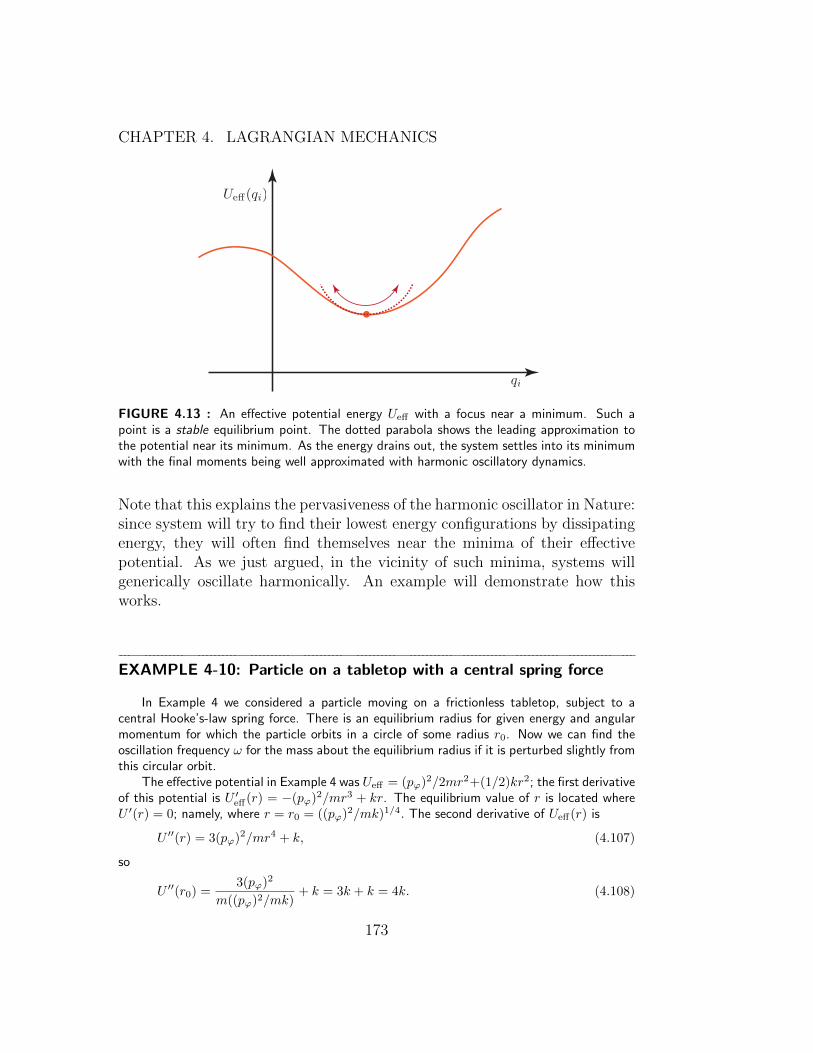
FIGURE 4.13 : An effective potential energy Ueff with a focus near a minimum. Such apoint is a stable equilibrium point. The dotted parabola shows the leading approximation tothe potential near its minimum. As the energy drains out, the system settles into its minimumwith the final moments being well approximated with harmonic oscillatory dynamics.

Note that this explains the pervasiveness of the harmonic oscillator in Nature:since system will try to find their lowest energy configurations by dissipatingenergy, they will often find themselves near the minima of their effectivepotential. As we just argued, in the vicinity of such minima, systems willgenerically oscillate harmonically. An example will demonstrate how thisworks.

EXAMPLE 4-10: Particle on a tabletop with a central spring force

In Example 4 we considered a particle moving on a frictionless tabletop, subject to acentral Hooke’s-law spring force. There is an equilibrium radius for given energy and angularmomentum for which the particle orbits in a circle of some radius r0. Now we can find theoscillation frequency ω for the mass about the equilibrium radius if it is perturbed slightly fromthis circular orbit.

The effective potential in Example 4 was Ueff = (pϕ)2/2mr2+(1/2)kr2; the first derivativeof this potential is U ′eff(r) = −(pϕ)2/mr3 + kr. The equilibrium value of r is located whereU ′(r) = 0; namely, where r = r0 = ((pϕ)2/mk)1/4. The second derivative of Ueff(r) is

U ′′(r) = 3(pϕ)2/mr4 + k, (4.107)

so

U ′′(r0) =3(pϕ)2

m((pϕ)2/mk)+ k = 3k + k = 4k. (4.108)

173

4.8. RELATIVISTIC GENERALIZATION

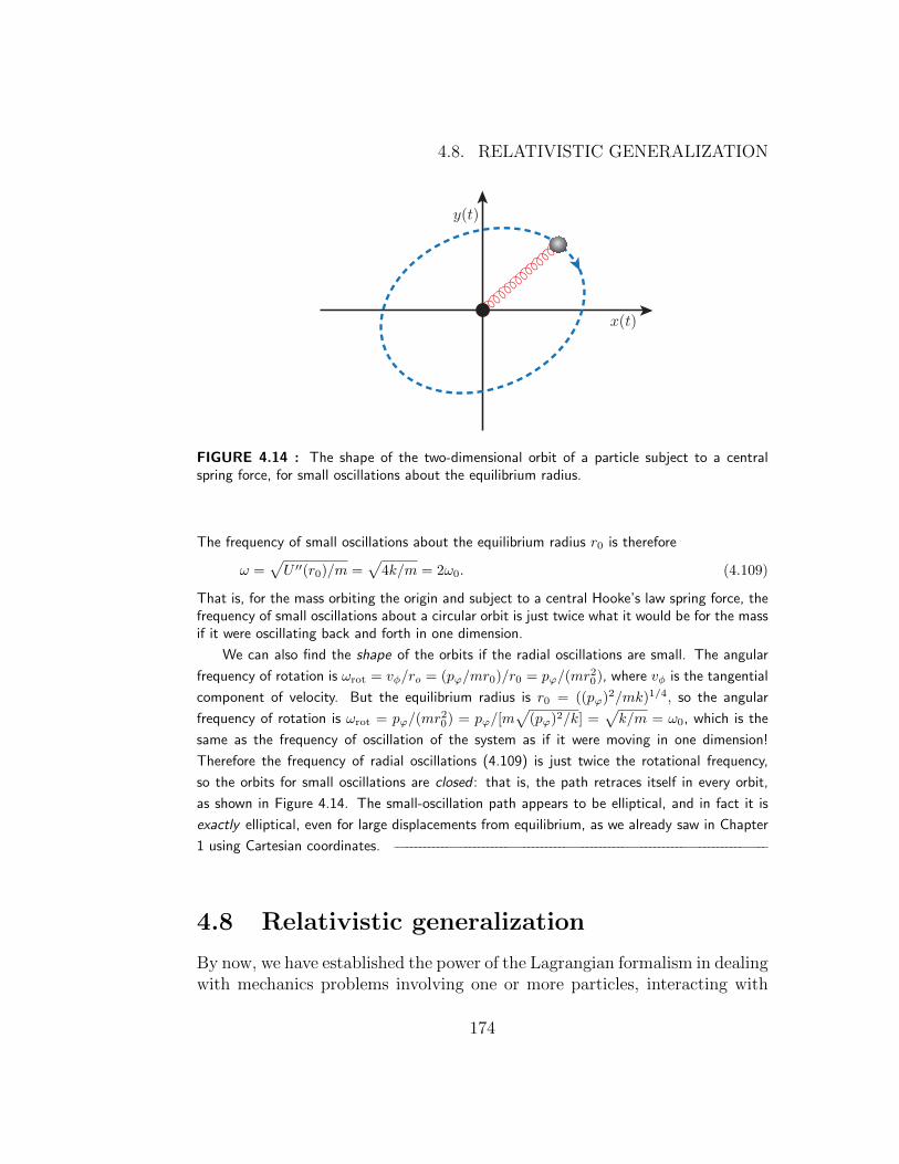
FIGURE 4.14 : The shape of the two-dimensional orbit of a particle subject to a centralspring force, for small oscillations about the equilibrium radius.

The frequency of small oscillations about the equilibrium radius r0 is therefore

ω =√U ′′(r0)/m =

√4k/m = 2ω0. (4.109)

That is, for the mass orbiting the origin and subject to a central Hooke’s law spring force, thefrequency of small oscillations about a circular orbit is just twice what it would be for the massif it were oscillating back and forth in one dimension.

We can also find the shape of the orbits if the radial oscillations are small. The angular

frequency of rotation is ωrot = vφ/ro = (pϕ/mr0)/r0 = pϕ/(mr20), where vφ is the tangential

component of velocity. But the equilibrium radius is r0 = ((pϕ)2/mk)1/4, so the angular

frequency of rotation is ωrot = pϕ/(mr20) = pϕ/[m

√(pϕ)2/k] =

√k/m = ω0, which is the

same as the frequency of oscillation of the system as if it were moving in one dimension!

Therefore the frequency of radial oscillations (4.109) is just twice the rotational frequency,

so the orbits for small oscillations are closed : that is, the path retraces itself in every orbit,

as shown in Figure 4.14. The small-oscillation path appears to be elliptical, and in fact it is

exactly elliptical, even for large displacements from equilibrium, as we already saw in Chapter

1 using Cartesian coordinates.

4.8 Relativistic generalization

By now, we have established the power of the Lagrangian formalism in dealingwith mechanics problems involving one or more particles, interacting with

174


conservative forces, with or without a large class of constraints. But allthis was within Newtonian mechanics — valid at speeds much less than thespeed of light. Can we use the Lagrangian formalism for situations requiringrelativistic treatment? The answer is rather simple to find. Our original setupfor deriving the Lagrangian formalism started by integrating proper time toconstruct the action functional (see equation (3.67))). We then took the limitof low speeds in (3.73 to identify a piece of the future Lagrangian — thekinetic energy. Through the example of a particle in a uniform gravitationalfield, we identified the second piece in L = T − U — the potential energy.We then proceeded to show that this works for any conservative potential,with one or more particles, with or without constraints. Going back to thebeginning, we then must have

L = T − U = mc2

√1− v2

c2− U (4.110)

to tackle a fully relativistic problem. We can even still write L = T − Uusing relativistic kinetic energy

T = mc2

√1− v2

c2−mc2 (4.111)

since the additional piece mc2 is a constant and hence does not effect theequations of motion. For a single particle in Cartesian coordinates, using ourresults from equations (3.72)), the equations of motion from (4.110 now looklike

d

dt(γx) = −∂U

∂x,

d

dt(γy) = −∂U

∂y,

d

dt(γz) = −∂U

∂z. (4.112)

This is the expected relativistic form of Newton’s second law from (2.93))or (2.100) if we identify F = −∇U . Hence, our entire Lagrangian formalismextends through the relativistic regime as long as we replace kinetic energyin L = T − U by (4.111 instead of T = (1/2)mv2.

There is, however, a possible new pitfall. As always, the LagrangianT − U is to be written from the perspective of an inertial observer. In rel-ativistic settings, the correct transformations linking inertial observers arethe Lorentz transformations. This implies that our Lagrangian should nowbe invariant under Lorentz transformations, not Galilean. The kinetic en-ergy term (4.111)) is indeed Lorentz invariant since it arises from the integral

175

4.9. SUMMARY

over proper time (see equation (3.67)). We thus have to make sure that thepotential energy term U in the Lagrangian is also Lorentz invariant, indepen-dently. Not any old force law is allowed! We will tackle the transformationproperties of the action in Chapter 6. And we will come back to this issuein Chapter 8 when we encounter a full Lorentz invariant force law — theelectromagnetic force. In the meantime, it is worthwhile emphasizing thattraditional mechanics force laws, such as Newtonian gravity, are not Lorentzinvariant and hence should only be considered in approximate Newtoniansettings with L = (1/2)mv2 − U — requiring only Galilean invariance fromthe action.

4.9 Summary

In this chapter we have presented a variational approach to classical mechan-ics, which is at the very heart of the subject. The variational approach is infact the central theme of this book.

We began the chapter by describing a conservative mechanical system byN generalized coordinates qk(t), with k = 1, 2, . . . , N , and then defining theLagrangian

L(t, q1, q2, ..., q1, q2, ...) = T − U (4.113)

as the difference between the kinetic and potential energies of the system,expressed in terms of the generalized coordinates qk, generalized velocities qk,and time t. We then define the action S[qk(t)] of the system as the functionalconsisting of the time integral over the Lagrangian L(t, q1, q2, ..., q1, q2, ...),from a starting time ta to an ending time tb,

S[qk(t)] =

∫ tb

ta

dt L(t, q1, q2, ..., q1, q2, ...) ≡∫ tb

ta

dt L(t, qk, qk) , (4.114)

where it is understood that the particle or system of particles begins at somedefinite position (q1, q2, ...)a at time ta and ends at some definite position(q1, q2, ...)b at time tb.

Hamilton’s principle then proposes that, for trajectories qk(t) wherethe action S is stationary — i.e., when

δS = δ

∫ tb

ta

L(t, qk, qk) dt = 0 (4.115)

176


the coordinates qk(t)’s satisfy the equations of motion for the system withthe prescribed boundary conditions at ta and tb. That is, the variationalprinciple δS = 0 gives the Lagrange equations

d

dt

∂L

∂qk− ∂L

∂qk= 0. (k = 1, 2, . . . , N) (4.116)

which are the differential equations of motion of the system.We also defined the Hamiltonian of the system to be

H ≡ qk pk − L (4.117)

where a sum over k is implied, and the generalized momenta pk are definedto be

pk =∂L

∂qk. (4.118)

Then

∂L

∂t= −dH

dt, (4.119)

so if L is not an explicit function of time, it follows that the Hamiltonian isconserved.

One of the strengths of the Lagrangian formalism is that it prescribes aquite straightforward algorithmic process to solve a problem. Here are thetypical steps:

1. Identify the degrees of freedom of each particle or object consistentwith any constraints, and choose an appropriate set of generalized co-ordinates qk for each.

2. Write the square of the velocity for each particle in terms of any conve-nient coordinates, usually Cartesian coordinates, in some inertial ref-erence frame. Then reexpress the kinetic energy in terms of the gen-eralized coordinates qk, the generalized velocities qk, and the time (ifneeded); i.e., , v2 = v2(qk, qk, t). Then write the total kinetic energy Tin terms of these v’s.

3. Write the total potential energy in the form U = U(qk, t).

4. Write the Lagrangian L(t, q1, q2, ..., q1, q2, ...) = T − U

177

4.9. SUMMARY

5. Identify any cyclic coordinates in L; that is, identify any coordinateql missing in the Lagrangian, even though its corresponding general-ized velocity ql is present. In this case the corresponding generalizedmomentum pl ≡ ∂L/∂ql is conserved. This gives a highly-valued firstintegral of motion, i.e., , a differential equation that is first order ratherthan second order.

6. If L is not an explicit function of time, then the Hamiltonian H ≡qk pk−L is conserved, providing another first integral of motion. Herethe generalized momentum pi = ∂L/∂qi.

7. If there are more generalized coordinates in the problem than firstintegrals identified in the preceding steps, then one or more of theLagrange equations of motion

∂L

∂qk− d

dt

∂L

∂qk= 0. (4.120)

must be used as well, to obtain a complete set of differential equations.That is, if there are N generalized coordinates, we will generally needN mutually independent differential equations whose solutions will givethe coordinates as functions of time. Some of these may be first-orderequations, each corresponding to a conserved quantity, while othersmay be second-order equations.

If the problem is simple, exact analytic solutions of the equations may bepossible. If not, we can always solve the equations numerically on a computer.There is also a very common intermediate situation, when one or more of theequations is too difficult to solve exactly, but approximate analytic techniquescan be used to find the answer as accurately as required. Finding a sufficientlyaccurate approximate analytic technique to solve a particular problem canbe very entertaining, requiring as much creativity as setting up the physicalproblem in the first place. One of the pleasures of doing physics is to finda way, no holds barred, to solve a problem to the extent we need it solved,using back-of-the-envelope calculations, dimensional reasoning, approximateanalytical techniques, numerical calculations, or whatever it takes to get thejob done.

178


Problems

PROBLEM 4-1: Example 2 featured a bead sliding on a vertically-oriented helix of radiusR. The angle θ about the symmetry axis was related to its vertical coordinate z on thewire by θ = αz. There is a uniform gravitational field g vertically downward. (a) Rewritethe Lagrangian and find the Lagrange equation, using z as the generalized coordinate. (b)Are there any conserved dynamical quantities? (c) Write the simplest differential equation ofmotion of the bead, and go as far as you can to solve analytically for the z as a function oftime.

PROBLEM 4-2: In Example 3 we found the equation of motion of a block on an inclinedplane, using the generalized coordinate s, the distance of the block from the bottom of theincline. Solve the equation for s(t), in terms of an arbitrary initial position s(0) and velocitys(0).

PROBLEM 4-3: A bead of mass m is placed on a vertically-oriented circular hoop of radiusR and negligible mass that is free to rotate about a vertical axis through its center. Thereis a uniform downward-directed gravitational field g. (a) Using polar and azimuthal angles θand ϕ as generalized coordinates, find the kinetic and potential energies of the bead. (b) Findthe equations of motion using Lagrange’s equations. (c) Write down two first integrals of themotion. What is the physical significance of each?

PROBLEM 4-4: A particle of mass m slides inside a smooth hemispherical bowl of radius R.Beginning with spherical coordinates r, θ and ϕ to describe the dynamics, select generalizedcoordinates, write the Lagrangian, and find the differential equations of motion of the particle.

PROBLEM 4-5: A particle moves in a cylindrically symmetric potential V (r, z). Use cylin-drical coordinates r, θ, and z to parameterize the space.

(a) Write the Lagrangian for an unconstrained particle of mass m (using cylindrical coor-dinates) in the presence of this potential.

(b) Write the Lagrange equations of motion for r, θ and z.(c) Identify and cyclic coordinates, and write a first integral corresponding to each.

PROBLEM 4-6: A spring pendulum has the pendulum bob of mass m attached to a springof force-constant k and unstretched length R0. The pendulum is constrained to swing in avertical plane (i.e., two degrees of freedoms are at work).

(a) Write the Lagrangian for the blob. Do not forget the potential for the spring.(b) Write the equations of motion for θ and r. Stare at the resulting differential equations

and write me a brief thank you note for not asking you to solve them.

PROBLEM 4-7: A particle of mass m slides inside a smooth paraboloid of revolution whoseaxis of symmetry z is vertical. The surface is defined by the equation z = αr2, where z andr are cylindrical coordinates, and α is a constant. There is a uniform gravitational field g. (a)Select two generalized coordinates for m. (b) Find T,U, and L. (c) Identify any ignorable

179

4.9. SUMMARY

coordinates, and any conserved quantities. (d) Show that there are two first integrals ofmotion, and find the corresponding equations.

PROBLEM 4-8: Repeat the preceding problem for a particle sliding inside a smooth conedefined by z = αr.

PROBLEM 4-9: A spring pendulum features a pendulum bob of mass m attached to oneend of a spring of force-constant k and unstretched length R. The other end of the spring isattached to a fixed point on the ceiling. The pendulum is allowed to swing in a plane. User, the distance of the bob from the fixed point, and θ, the angle of the spring relative to thevertical, as generalized coordinates. (a) Find the kinetic and potential energies of the bob interms of the generalized coordinates and velocities. (b) Find the Lagrangian. Are there anyignorable coordinates? (c) Are there any conserved quantities? (d) Find a complete set ofequations of motion, including as many first integrals as possible.

PROBLEM 4-10: A pendulum is constructed from a bob of mass m on one end of a lightstring of length D. The other end of string is attached to the top of a circular cylinder ofradius R (R < 2D/π). The string makes an angle θ with the vertical, as shown below, asthe pendulum swings in the plane. There is a uniform gravity g directed downward. (a) Findthe Lagrangian and write out Lagrange’s equation using θ as the generalized coordinate. (b)Identify any first integrals of motion. (c) Find the frequency of small oscillations about thestable equilibrium point.

PROBLEM 4-11: A particle moves with a cylindrically symmetric potential energy U =U(r, z) where r, θ, z are cylindrical coordinates. (a) Write the Lagrangian for an unconstrainedparticle of mass m in this case. (b) Are there any cyclic coordinates? If so, what symmetriesdo they correspond to, and what are the resulting constants of the motion? (c) Write theLagrange equation for each cyclic coordinate. (d) Find the Hamiltonian H. Is it conserved?(e) Find the total energy E. Is E = H? is E conserved? (f) Write the simplest (i.e., ,lowest-order) complete set of differential equations of motion of the particle.

PROBLEM 4-12: A plane pendulum is made with a plumb bob of mass m hanging on aHooke’s-law spring of negligible mass, force constant k, and unstretched length `0. The springcan stretch but is not allowed to bend. There is a uniform downward gravitational field g.(a) Select generalized coordinates for the bob, and find the Lagrangian in terms of them. (b)Write out the Lagrange equations of motion (c) Are there any conserved quantities? If so,write down the corresponding conservation law(s). (d) If the bob is swinging back and forth,find the frequency of small oscillations in the general case where the spring can change itslength while the bob is swinging back and forth.

PROBLEM 4-13: Motion in a slowly-changing uniform electric field

A particle of mass m and charge q moves within a parallel-plate capacitor whose chargeQ is decays exponentially with time, Q = Q0e

−t/τ , where τ is the time constant of the decay.Find the equations of motion of the particle.

180


PROBLEM 4-14: A particle of mass m travels between two points x = 0 and x = x1 onEarth’s surface, leaving at time t = 0 and arriving at t = t1. The gravitational field g isuniform. (a) Suppose m moves along the ground (keeping altitude z = 0) at steady speed.Find the total action S to go by this path. (b) Suppose instead that m moves along theleast-action parabolic path. Show that the action in this case is

S =mx2

1

2t1− mg2t31

24(4.121)

and verify that it is less than the action for the straight-line path of part (a).

PROBLEM 4-15: Suppose the particle of the preceding problem moves instead at constantspeed along a isoceles triangular path between the beginning point and the end point, with thehigh point at height z1 above the ground, at x = x1/2 and t = t1/2. (a) Find the action forthis path. (b) Find the altitude z1 corresponding to the least-action path among this class ofconstant-speed triangular paths. (c) Verify that the total action for this path is greater thanthat of the parabolic path of the preceding problem.

PROBLEM 4-16: A plane pendulum consists of a light rod of length R supporting a plumbbob of mass m in a uniform gravitational field g. The point of support of the top end of therod is forced to oscillate back and forth in the horizontal direction with x = A cosωt. Usingthe angle θ of the bob from the vertical as the generalized coordinate, (a) find the Lagrangianof the plumb bob. (b) Are there any conserved dynamical quantities? (c) Find the simplestdifferential equation of motion of the bob.

PROBLEM 4-17: Solve the preceding problem if instead of being forced to oscillate in thehorizontal direction, the upper end of the rod is forced to oscillate in the vertical direction withy = A cosωt.

PROBLEM 4-18: A particle of mass m on a frictionless table top is attached to one endof a light string. The other end of the string is threaded through a small hole in the tabletop, and held by a person under the table. If given a sideways velocity v0, the particle circlesthe hole with radius r0. At time t = 0 the mass reaches an angle defined to be θ = 0 onthe table top, and the person under the table pulls on the string so that the length of thestring above the table becomes r(t) = r0 − αt for a period of time thereafter, where α is aconstant. Using θ as the generalized coordinate of the particle, find its Lagrangian, identifyany conserved quantities, finds its simplest differential equation of motion, and get as far asyou can using analytic means alone toward finding the solution θ(t) (or t(θ) ).

PROBLEM 4-19: A rod is bent in the middle by angle α. The bottom portion is kept verticaland the top portion is therefore oriented at angle α to the vertical. A bead of mass m is slippedonto the top portion and the bottom portion is forced by a motor to rotate at constant angularspeed ω about the vertical axis. (a) Define a generalized coordinate for the bead and writedown the Lagrangian. (b) Identify any conserved quantity or quantitiies and explain why it (orthey) are conserved. (c) Find the generalized momentum of the bead and the Hamiltonian.(d) Are there any equilibrium points of the bead? If so, are they stable or unstable?

181

4.9. SUMMARY

PROBLEM 4-20: A wire is bent into the shape of a cycloid, defined by the parametricequations x = A(ϕ+ sinϕ) and y = A(1− cosϕ), where ϕ is the parameter (−π < ϕ < π),and A is a constant. The wire is in a vertical plane, and is spun at constant angular velocityω about a vertical axis through its center. A bead of mass m is slipped onto the wire. (a)Find the Lagrangian of the bead, using the parameter ϕ as the generalized coordinate. (b)Identify any first integral of motion of the bead. (c) Are there any equilibrium points of thebead? Are they stable or unstable? For any stable equilibrium point, find the frequency ofsmall oscillations about that point.

PROBLEM 4-21: Center of mass and relative coordinates. Show that for two particles movingin one dimension, with coordinates x1 and x2, with a potential that depends only upon theirseparation x2 − x1, then the Lagrangian

L =1

2m1x

21 +

1

2m2x

22 − U(x2 − x1) (4.122)

can be rewritten in the form

L =1

2MX2 +

1

2µx′2 − U(x′), (4.123)

where M = m1 + m2 is the total mass and µ = m1m2/M is the “reduced mass” of thesystem, and X = (m1x1 + m2x2)/M is the center of mass coordinate and x′ = x2 − x1 isthe relative coordinate.

PROBLEM 4-22: Two blocks of equal mass m, connected by a Hooke’s-law spring of un-stretched length `, are free to move in one dimension. Find the equations of motion of thesystem, using the relative and center of mass coordinates introduced in the preceding problem.

PROBLEM 4-23: A small block of mass m and a weight of mass M are connected by a stringof length D. The string has been threaded through a small hole in a tabletop, so the block canslide without friction on the tabletop, while the weight hangs vertically beneath the tabletop.We can let the hole be the origin of coordinates, and use polar coordinates r, θ for the block,where r is the block’s distance from the hole, and z for the distance of the weight below thetabletop. (a) Using generalized coordinates r and θ, write down the Lagrangian of the systemof block plus weight. (b) Write down a complete set of first integrals of the motion, explainingthe physical meaning of each. (c) Show that the first integrals can be combined to give anequation of the form

E =1

2(M +m)r2 + Ueff(r) (4.124)

and write out an expression for Ueff(r). (d) Find the radius of a circular orbit of the block interms of constants of the motion. (e) Now suppose the block executes small oscillations abouta circular orbit. What is the frequency of these oscillations? Is the resulting orbit of the blockopen or closed? That is, does the perturbed orbit of the block continually return to its formerposition or not?

182


PROBLEM 4-24: The Moon has no atmosphere, so it would be possible in principle to shootprojectiles off its surface with the escape velocity or even higher. The projectiles might be minedMoon material, shot into space to use as raw material for building structures there. One way toraise material to the escape velocity would be to construct a huge boom that would continuallyswing around in a horizontal plane with constant angular velocity ω. Buckets of material wouldbe dropped onto the boom at some small distance r0 from the rotation axis, with no initialradial velocity. The buckets would then be thrown outward by the boom’s rotation and wouldcome off the end of the boom with the escape velocity if the boom is long enough and if ωis large enough. (a) Find the Lagrangian for a bucket of material of mass m. (b) Find itsequation of motion. (c) Solve it for r(t), subject to the given initial conditions (i.e., , be surethat r = r0 and r = 0 at t = 0.) (d) If the boom has radius R, find the radial and tangentialcomponents of the bucket’s velocity, and its total speed, as it emerges from the end of theboom. (e) Find the power input P = dE/dt into a bucket of mass m as a function of time.Is the power input larger at the beginning or end of the bucket’s journey along the boom? (f)Find the torque exerted by the boom on the bucket, as a function of the position r of thebucket on the boom. There would be an equal but opposite torque back on the boom, causedby the bucket, which might break the boom. At what part of the bucket’s journey would thistorque most likely break the boom? (g) If R = 100 meters and r0 = 1 meter, what must bethe rotational period of the boom so that buckets will reach the Moon’s escape speed as theyfly off the boom?

PROBLEM 4-25: Consider a vertical circular hoop of radius R rotating about a vertical axiswith constant angular velocity Ω. A bead of mass m is threaded on the hoop. Denote theangle along the hoop of the bead as measured from the vertical as θ.

(a) Write the Lagrangian and equations of motion.

(b) For small angles θ 1 (in radians), we have the approximate expressions cos θ ∼ 1and sin θ ∼ θ. In this regime, simplify the equation of motion for θ. Say a sentence about thesolution θ(t) that you expect.

(c) In the result of part (a), rewrite things in terms of the new coordinate α ≡ θ−π. Notethe mildly exciting identities cos(α + π) = − cosα and sin(α + π) = − sinα. Now considerthe regime α ∼ 0 and simplify the equation of motion for α.

PROBLEM 4-26: Consider the Lagrangian L′ = m x y− k x y for a particle free to move intwo dimensions, where x and y are Cartesian coordinates, and m and k are constants.

(a) Find the equations of motion for the system.

(b) Confirm that the answer to part (a) is the same if we were to use instead the Lagrangianfor the harmonic oscillator L = (1/2)m(x2 + y2)− (1/2)k(x2 + y2).

(c) Show that L and L′ do not differ by a total derivative!

PROBLEM 4-27: In certain situations, it is possible to incorporate frictional effects in a simpleway into a Lagrangian problem. As an example, consider the Lagrangian

L = eγt(

1

2mq2 − 1

2kq2

). (4.125)

183

4.9. SUMMARY

(a) Find the equation of motion for the system.(b) Do a coordinate change s = eγt/2q. Rewrite the dynamics in terms of s.(c) How would you describe the system?

PROBLEM 4-28: Consider a particle moving in three dimensions with Lagrangian L =(1/2)m(x2 + y2 + z2)+ax = b, where a and b are constants. (a) Find the equations of motionand show that the particle moves in a straight line at constant speed, so that it must be a freeparticle. (b) The result of (a) shows that there must be another reference frame (x′, y′, z′) suchthat the Lagrangian is just the usual free-particle Lagrangian L′ = (1/2)m(x′2 + y′2 + z′2).However, L′ may also be allowed an additive constant, which cannot show up in Lagrange’sequations. Find the Galilean transformation between (x, y, z) and (x′, y′, z′) and find thevelocity of the new primed frame in terms of a and b.

PROBLEM 4-29: Consider a Lagrangian L′ = L + df/dt, where the Lagrangian is L =L(t, qk, qk), and the function f = f(qk, t). (a) Show that L′ = L′(qk, qk, t), so that itdepends upon the proper variables. Show that this would not generally be true if f wereallowed to depend upon the q′ks. (b) Show that L′ obeys Lagrange’s equations if L does, bysubstituting L′ into Lagrange’s equations. Therefore the equations of motion are the sameusing L′ as using L, so the Lagrangian of a particle is not unique. (This problem requires carein taking total and partial derivatives!)

PROBLEM 4-30: Show that the function L′ given in the preceding problem must obey La-grange’s equations if L does, directly from the principle of stationary action. Lagrange’sequations do not have to be written down for this proof!

PROBLEM 4-31: Consider the Lagrangian L′ = mxy − kxy for a particle free to movein two dimensions, where x and y are Cartesian coordinates, and m and k are constants.(a) Show that his Lagrangian gives the equations of motion appropriate for a two-dimensionsimple harmonic oscillator. Therefore as far as the motion of the particle is concerned, L′ isequivalent to L = (1/2)m(x2 + x2)− (1/2)k(x2 + y2). (b) Show that L′ and L do not differby the total time derivative of any function f(x, y). Therefore L′ is not a member of theclass of Lagrangians mentioned in the preceding problems, so there are even more Lagrangiansdescribing a particle than suggested before.

PROBLEM 4-32: Consider a Lagrangian that depends on second derivatives of the coordi-nates

L = L(qk, qk, qk, t) . (4.126)

Through the variational principle, show that the resulting differential equations of motion arethird order in the time derivative.

PROBLEM 4-33: A pendulum consists of a plumb bob of mass m on the end of a string thatswings back and forth in a plane. The upper end of the string passes through a small hole inthe ceiling, and the angle θ of the bob relative to the vertical changes with time as it swingsback and forth. The string is pulled upward at constant rate through the hole, so the length

184


R of the pendulum decreases at a constant rate, with dR/dt = −α. (a) Find the Lagrangianof the bob, using θ as the generalized coordinate. (b) Find the Hamiltonian H. Is H equal tothe energy E? Why or why not? (c) Is either H or E conserved? Why or why not?

PROBLEM 4-34: A spherical pendulum consists of a particle of mass m on the end of astring of length R. The position of the particle can be described by a polar angle θ and anazimuthal angle ϕ. The length of the string decreases at the rate dR/dt = −f(t), wheref(t) is a positive function of time. (a) Find the Lagrangian of the particle, using θ and ϕ asgeneralized coordinates. (b) Find the Hamiltonian H. Is H equal to the energy? Why of whynot? (c) Is either E or H conserved? Why or why not?

PROBLEM 4-35: Equation 4.100 for the Hamiltonian of a bead on a parabolic wire turningwith constant angular velocity ω is

H =1

2m[(1 + 4α2r2)r2 − r2ω2] +mgαr2, (4.127)

where H is a constant. Reduce the problem to quadrature: That is, find an equation for thetime t is terms of an integral over r.

PROBLEM 4-36: A bead of mass m is placed on a vertically-oriented circular hoop of radiusR that is forced to rotate with constant angular velocity ω about a vertical axis through itscenter. (a) Using the polar angle θ measured up from the bottom as the single generalizedcoordinate, find the kinetic and potential energies of the bead. (Remember that the bead hasmotion due to the forced rotation of the hoop as well as motion due to changing θ. ) (b) Findthe bead’s equation of motion using Lagrange’s equation. (c) Is its energy conserved? Whyor why not? (c) Find its Hamiltonian. Is H conserved? Why or why not? (d) Is E = H?Why or why not? (e) Find the equilibrium angle θ0 for the bead as a function of the hoop’sangular velocity ω. Sketch a graph of θ0 versus ω. Notice that there is a “phase transition” ata certain critical velocity ωcrit. (b) Find the frequency of small oscillations of the bead aboutthe equilibrium angle θ0, as a function of ω.

PROBLEM 4-37: A bead of mass m is placed on a vertically-oriented elliptical hoop that isforced to rotate with constant angular velocity ω about a vertical axis through its center. Theellipse is defined by (x/a)2 + (y/b)2 = 1 where a and b are the semimajor and semiminor axesof the ellipse, and suppose that the vertical axis is the semiminor axis. (a) Choose a generalizedcoordinate for the bead and find the Lagrangian (b) Is the bead’s energy conserved? Why orwhy not? (c) Is the bead’s angular momentum conserved about the vertical axis? Why or whynot? (d) Find the bead’s Hamiltonian. Is H conserved? Why or why not? (d) Is E = H?Why or why not? (e) Given ω, is there an equilibrium position of the bead, and is it stable orunstable?

PROBLEM 4-38: In Example 9 we analyzed the case of a bead on a rotating parabolic wire.The energy of the bead was not conserved, but the Hamiltonian was:

H =1

2m(1 + 4α2r2)r2 + “U ′′eff = constant,

185

4.9. SUMMARY

where

“U ′′eff =1

2mr2(2gα2 − ω2).

There is an equilibrium point at r = 0 which is unstable if ω > ω0 ≡√

2g α, neutrally stable ifω = ω0, and stable if ω < ω0. Find the frequency of small oscillations about r = 0 if ω < ω0.Hint: Note that for very small oscillations near r = 0 the quantity (1 + 4α2r2) ∼= 1 to anexcellent approximation, so the Hamiltonian is

H ∼=1

2mr2 +

1

2kr2

where the constant k = m(2gα2 − ω2).

186

Appendix A

When is H 6= E?

In Example 9 the Hamiltonian H was not equal to E. Why were they differ-ent, and why was H conserved while E was not?

The definition H = qk∂L/∂qk−L (using the Einstein summation conven-tion, implying a sum over k in the first term on the right since k is repeatedin that term) contains the Lagrangian L = T − U , where only the kineticenergy T depends upon the generalized velocities qk; therefore

H = qk∂T

∂qk+ U − T. (A.1)

Now let r(qk, t) be the position vector of the particle from some arbitraryorigin fixed in an inertial frame, in terms of the time and any or all of thegeneralized coordinates qk. Then the velocity of the particle is

v =dr(qk, t)

dt=∂r

∂t+∂r

∂qlql, (A.2)

because r can change with time either from an explicit time dependenceor because one or more of the generalized coordinates changes with time.Therefore its kinetic energy is T = (1/2)mv2 = (1/2)mv · v, which is

T =1

2

[m∂r

∂t· ∂r∂t

+ 2∂r

∂t· ∂r∂ql

ql +∂r

∂qlql ·

∂r

∂qmqm

](A.3)

where we have used a different dummy summation index m in the final factorto distinguish it from the sum over l is the preceding factor. That is, by theEinstein summation convention the final term above is actually the product of

187

APPENDIX A. WHEN IS H 6= E?

two sums, one over l and one over m. Now we can take the partial derivativeof T with respect to a particular one of the generalized velocities qk,

∂T

∂qk=

1

2m

[2∂r

∂t· ∂r∂qk

+ 2∂r

∂qk· ∂r∂ql

ql

](A.4)

where there is a factor of two in the second term because qk occurs in bothsummations in the last term of the expression for T . Therefore the sum

qk∂T

∂qk= m

[∂r

∂t· ∂r∂qk

qk +∂r

∂qkqk ·

∂r

∂qlql

]= 2T −m∂r

∂t·[∂r

∂t+∂r

∂qkqk

]= 2T −m∂r

∂t· drdt, (A.5)

using equations (A.3)) and (A.4. The HamiltonianH can therefore be written

H = E −mdr

dt· ∂r∂t

= E − p · ∂r∂t

(A.6)

where p is the momentum of the particle in the chosen inertial frame. If thetransformation r = r(qk, t) between the Cartesian coordinates r = (x, y, z)and the generalized coordinates qk happens not to be an explicit function oftime, i.e., , if ∂r/∂t = 0, then the Hamiltonian is just T + U . This caseoccurs when there are no constraints or when any constraints are fixed inspace. But if the constraints are moving, then the transformation r = r(qk, t)does generally depend upon time, and so in the likely case that there isa component of ∂r/∂t in the direction of the particle’s momentum p, theHamiltonian is not equal to T + U .

For the problem of the bead on a rotating parabolic wire, where theconstraint is obviously moving, the position vector of the bead can be takento be r = (x, y, z) = (r cosωt, r sinωt, αr2). In that case we found thatH = T+U−mω2r2, and it is easy to show that mω2r2 = p·∂r/∂t, as requiredby equation (A.6)). It is clear that E is not conserved in this case becausethe rotating wire is continually doing work on the bead. The wire exerts aforce F θ in the tangential direction, which causes work to be done at therate dW/dt = F θvθ = F θrω. From the elementary relationship N z = dLz/dt,with torque N z = F θr and angular momentum Lz = (r × pz = mr2ω, itfollows that

dW

dt= ω

d(mr2ω)

dt= mω2dr

2

dt, (A.7)

APPENDIX A. WHEN IS H 6= E?

so that the work done by the wire is W = mω2r2 plus a constant of in-tegration, which depends upon the initial location of the bead. Thus theenergy’ E = T + U of the bead increases by the work done upon it by thewire, so that E minus the work done must be conserved, and that differenceE −mω2r2 = H.

Note that:

1. H is conserved if the Lagrangian L is not an explicit function of time.

2. H = E if the coordinate transformation r = r(qk, t) is not an explicitfunction of time. Therefore it is possible to have E = H, with both Eand H conserved, or neither conserved, and it is also possible to haveE 6= H, with both conserved, neither conserved, or only one of the twoconserved. Examples are given in the problems.

189

chapter 4 lagrangian mechanics - department of physics...

Documents