chapter 5 data collection and analysis...
TRANSCRIPT
78
CHAPTER 5
DATA COLLECTION AND ANALYSIS
INTRODUCTION
In this research, primary data collection is done through survey. A simple structured
non-disguised questionnaire is used to collect primary data. Data collection through
questionnaire is more useful when data are to be collected from large number of
respondents. Other benefits of questionnaire tool are – these help to collect data from
geographically wide-spread respondents i.e. respondents from across the district or
state or country. There is no interviewers’ bias. Respondents can take their own time
to think and answer the questions at their convenient.
Accurate data analysis was possible in this research due to pilot study. Necessary
corrections were made in the questionnaire after analyzing pilot study data.
Incomplete questionnaires or the questionnaires with unanswered questions are
discarded. Data editing and coding is done before making data entry in SPSS.
5. 1. Variables
Variables are in relations to awareness, perceptions, and preferences on marketing
communications tools such as Calls, SMS, Spam/Junk, Catalogs/Brochures, Do Not
Call Registry, Consumer Dispute Redressal Commission, and Consumer Protection
Act, respondents’ age, education, occupation, gender, income etc.
5.1.1. Classification of Variables:
Variables are classified according to customers’ Awareness, Perceptions, and
Preferences of marketing communications tools.
79
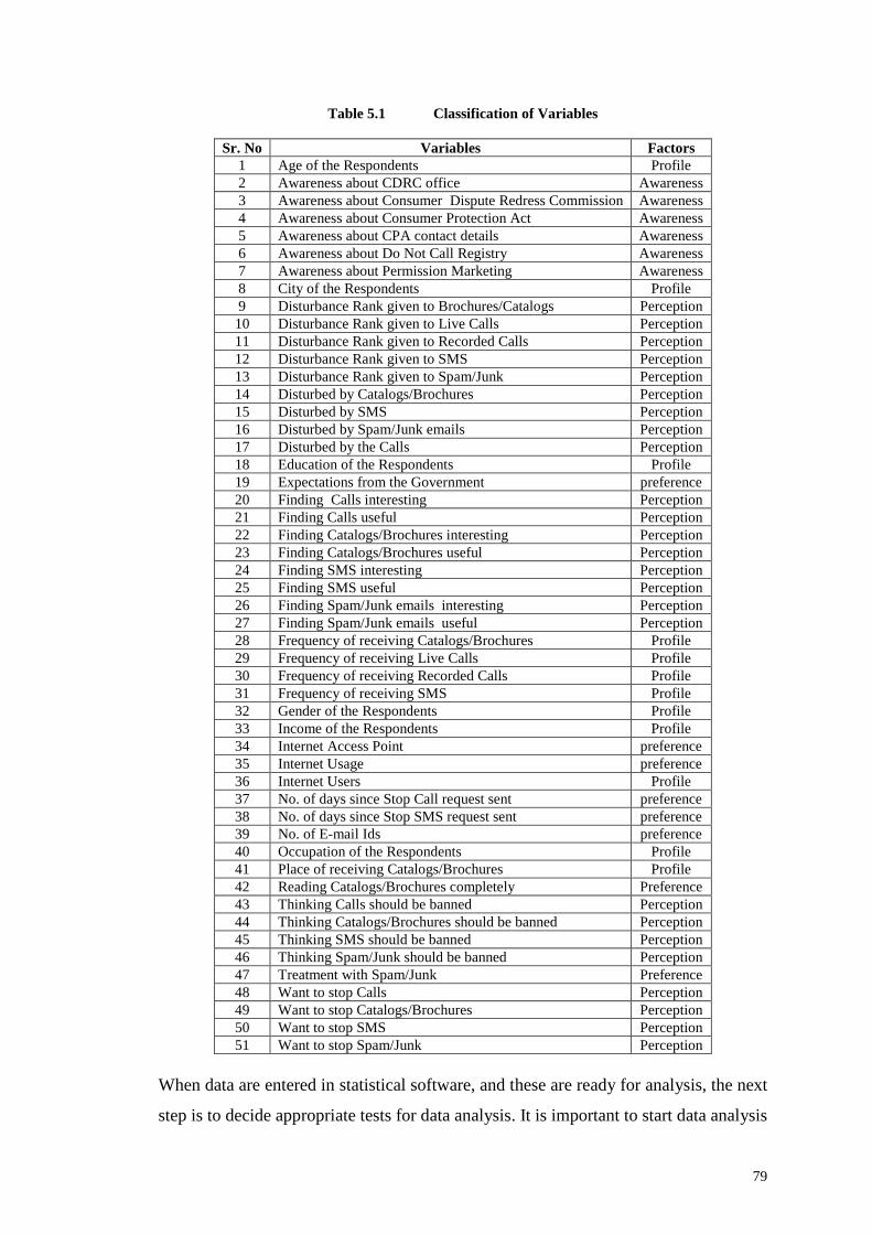
Table 5.1 Classification of Variables
Sr. No Variables Factors1 Age of the Respondents Profile2 Awareness about CDRC office Awareness3 Awareness about Consumer Dispute Redress Commission Awareness4 Awareness about Consumer Protection Act Awareness5 Awareness about CPA contact details Awareness6 Awareness about Do Not Call Registry Awareness7 Awareness about Permission Marketing Awareness8 City of the Respondents Profile9 Disturbance Rank given to Brochures/Catalogs Perception10 Disturbance Rank given to Live Calls Perception11 Disturbance Rank given to Recorded Calls Perception12 Disturbance Rank given to SMS Perception13 Disturbance Rank given to Spam/Junk Perception14 Disturbed by Catalogs/Brochures Perception15 Disturbed by SMS Perception16 Disturbed by Spam/Junk emails Perception17 Disturbed by the Calls Perception18 Education of the Respondents Profile19 Expectations from the Government preference20 Finding Calls interesting Perception21 Finding Calls useful Perception22 Finding Catalogs/Brochures interesting Perception23 Finding Catalogs/Brochures useful Perception24 Finding SMS interesting Perception25 Finding SMS useful Perception26 Finding Spam/Junk emails interesting Perception27 Finding Spam/Junk emails useful Perception28 Frequency of receiving Catalogs/Brochures Profile29 Frequency of receiving Live Calls Profile30 Frequency of receiving Recorded Calls Profile31 Frequency of receiving SMS Profile32 Gender of the Respondents Profile33 Income of the Respondents Profile34 Internet Access Point preference35 Internet Usage preference36 Internet Users Profile37 No. of days since Stop Call request sent preference38 No. of days since Stop SMS request sent preference39 No. of E-mail Ids preference40 Occupation of the Respondents Profile41 Place of receiving Catalogs/Brochures Profile42 Reading Catalogs/Brochures completely Preference43 Thinking Calls should be banned Perception44 Thinking Catalogs/Brochures should be banned Perception45 Thinking SMS should be banned Perception46 Thinking Spam/Junk should be banned Perception47 Treatment with Spam/Junk Preference48 Want to stop Calls Perception49 Want to stop Catalogs/Brochures Perception50 Want to stop SMS Perception51 Want to stop Spam/Junk Perception
When data are entered in statistical software, and these are ready for analysis, the next
step is to decide appropriate tests for data analysis. It is important to start data analysis
80
with knowing nature and characteristics of data. The measurement scales used while
collecting information from respondents will help in deciding selection of statistical
tests. Parametric tests can be used only when following four assumptions are met:
1. Data measured at least Interval scale
2. Variables are normally distributed
3. Data are independent
4. Distribution has equal variance
In the present research, measurement scales used are nominal, and ordinal. Data are
nonmetric and information is collected from one sample. First assumption in above
list is not met. To check second assumption about normality Histograms with normal
curve and K-S tests are used as parts of Univariate technique.
5. 2. FREQUENCY, MEASURES OF ASSOCIATION, AND HISTOGRAMSWITH NORMAL CURVE
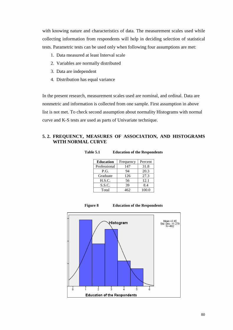
Table 5.1 Education of the Respondents
Figure 8 Education of the Respondents
Education Frequency PercentProfessional 147 31.8
P.G. 94 20.3Graduate 126 27.3H.S.C. 56 12.1S.S.C. 39 8.4Total 462 100.0
81
Majority respondents (31 %) are professionals by education (CA/MBA etc.) followed
by Graduates (27 %), Postgraduates (20 %), HSC (12 %), and SSC (8 %).
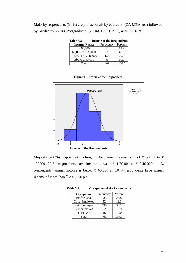
Table 5.2 Income of the Respondents
Figure 9 Income of the Respondents
Majority (48 %) respondents belong to the annual income slab of ` 60001 to `
120000. 29 % respondents have income between ` 1,20,001 to ` 2,40,000, 11 %
respondents’ annual income is below ` 60,000 an 10 % respondents have annual
income of more than ` 2,40,000 p.a.
Table 5.3 Occupation of the Respondents
Income (` p.a.) Frequency Percent< 60,000 55 11.9
60,001 to 1,20,000 223 48.31,20,001 to 2,40,000 138 29.9
Above 2,40,000 46 10.0Total 462 100.0
Occupation Frequency PercentProfessional 133 28.8
Govt. Employee 52 11.3Pvt. Employee 139 30.1Self-employed 92 19.9
House-wife 46 10.0Total 462 100.0
82
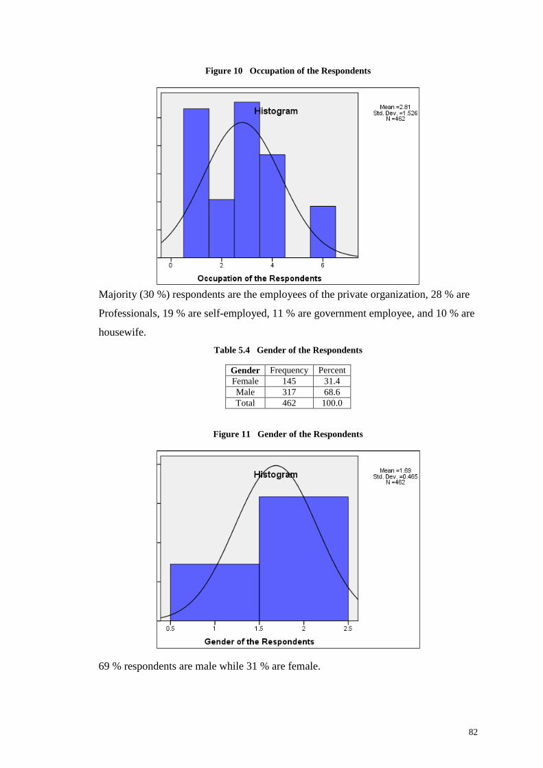
Figure 10 Occupation of the Respondents
Majority (30 %) respondents are the employees of the private organization, 28 % are
Professionals, 19 % are self-employed, 11 % are government employee, and 10 % are
housewife.
Table 5.4 Gender of the Respondents
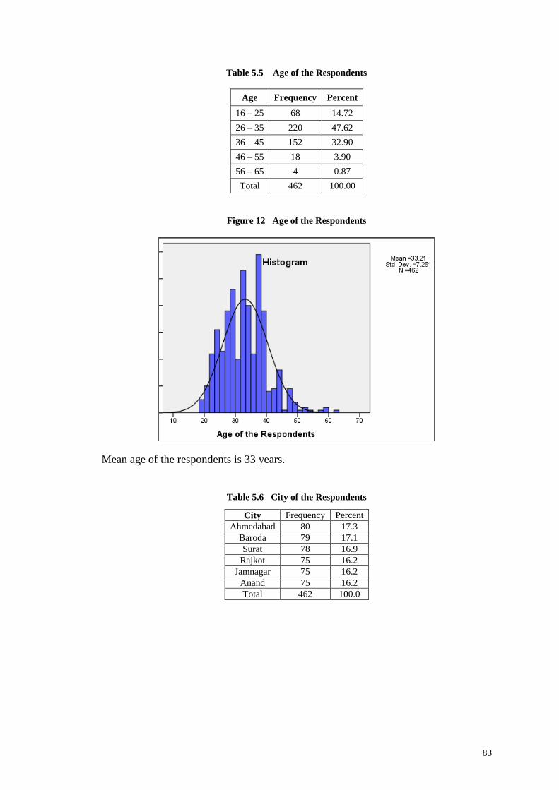
Figure 11 Gender of the Respondents
69 % respondents are male while 31 % are female.
Gender Frequency PercentFemale 145 31.4Male 317 68.6Total 462 100.0
83
Table 5.5 Age of the Respondents
Age Frequency Percent
16 – 25 68 14.72
26 – 35 220 47.62
36 – 45 152 32.90
46 – 55 18 3.90
56 – 65 4 0.87
Total 462 100.00
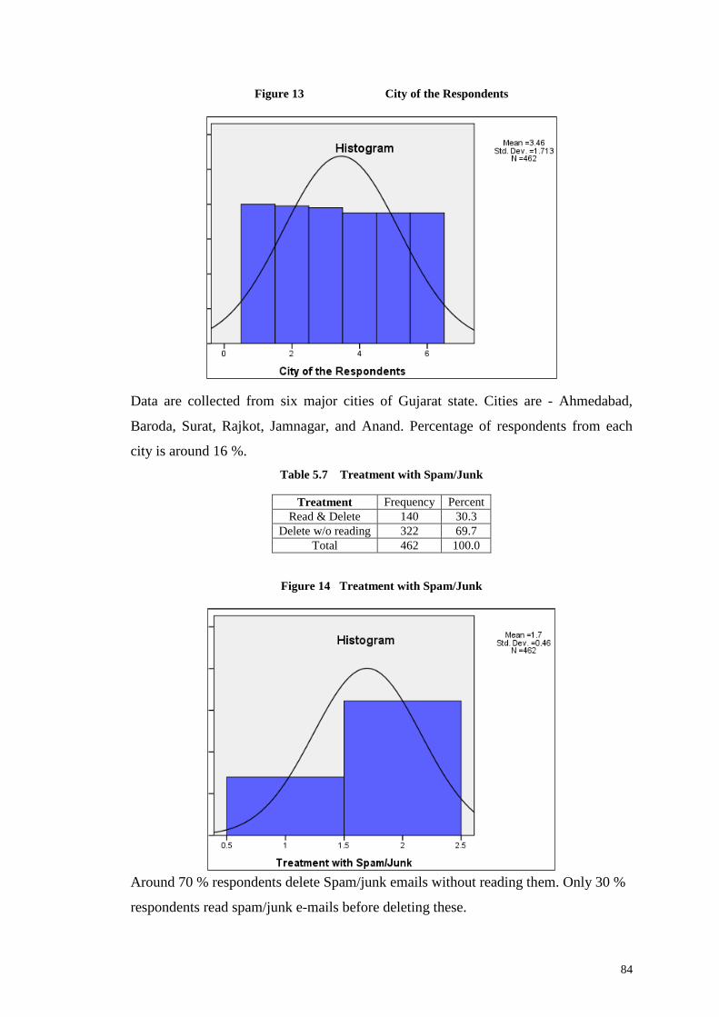
Figure 12 Age of the Respondents
Mean age of the respondents is 33 years.
Table 5.6 City of the Respondents
City Frequency PercentAhmedabad 80 17.3
Baroda 79 17.1Surat 78 16.9
Rajkot 75 16.2Jamnagar 75 16.2
Anand 75 16.2Total 462 100.0
84
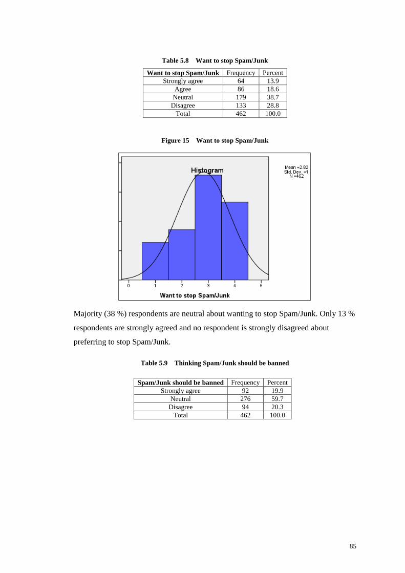
Figure 13 City of the Respondents
Data are collected from six major cities of Gujarat state. Cities are - Ahmedabad,
Baroda, Surat, Rajkot, Jamnagar, and Anand. Percentage of respondents from each
city is around 16 %.
Table 5.7 Treatment with Spam/Junk
Figure 14 Treatment with Spam/Junk
Around 70 % respondents delete Spam/junk emails without reading them. Only 30 %
respondents read spam/junk e-mails before deleting these.
Treatment Frequency PercentRead & Delete 140 30.3
Delete w/o reading 322 69.7Total 462 100.0
85
Table 5.8 Want to stop Spam/Junk
Figure 15 Want to stop Spam/Junk
Majority (38 %) respondents are neutral about wanting to stop Spam/Junk. Only 13 %
respondents are strongly agreed and no respondent is strongly disagreed about
preferring to stop Spam/Junk.
Table 5.9 Thinking Spam/Junk should be banned
Want to stop Spam/Junk Frequency PercentStrongly agree 64 13.9
Agree 86 18.6Neutral 179 38.7
Disagree 133 28.8Total 462 100.0
Spam/Junk should be banned Frequency PercentStrongly agree 92 19.9
Neutral 276 59.7Disagree 94 20.3
Total 462 100.0
86
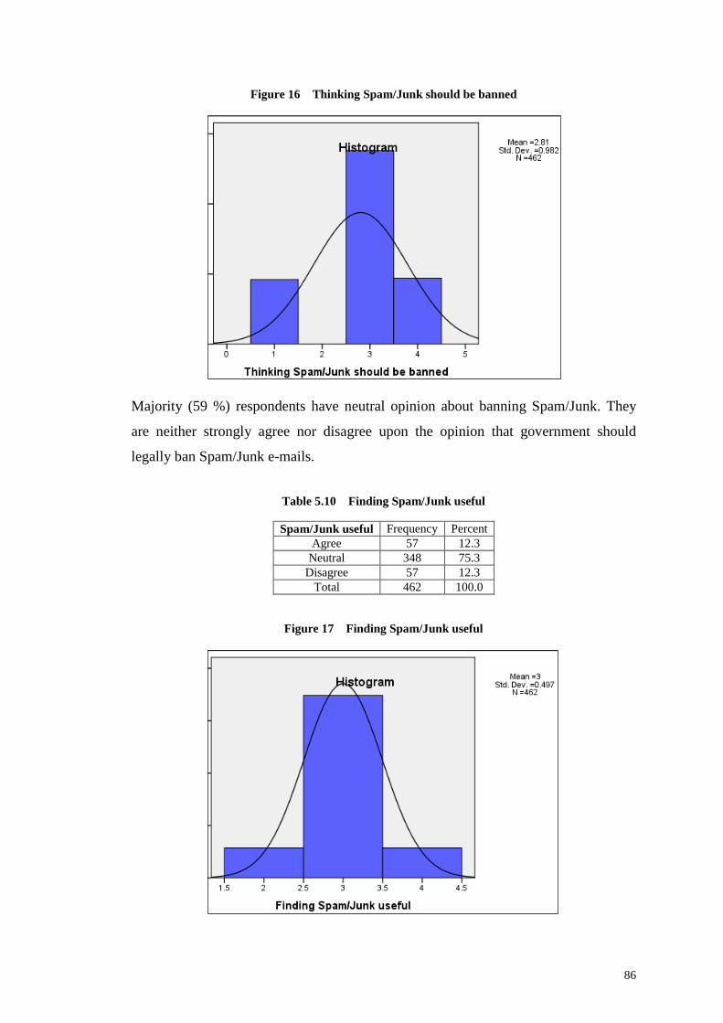
Figure 16 Thinking Spam/Junk should be banned
Majority (59 %) respondents have neutral opinion about banning Spam/Junk. They
are neither strongly agree nor disagree upon the opinion that government should
legally ban Spam/Junk e-mails.
Table 5.10 Finding Spam/Junk useful
Figure 17 Finding Spam/Junk useful
Spam/Junk useful Frequency PercentAgree 57 12.3
Neutral 348 75.3Disagree 57 12.3
Total 462 100.0
87
Majority (75 %) respondents are neutral about usefulness of Spam/Junk. They neither
agree nor disagree that Spam/Junk e-mails are useful.
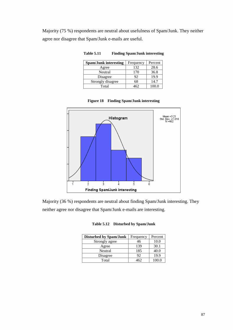
Table 5.11 Finding Spam/Junk interesting
Figure 18 Finding Spam/Junk interesting
Majority (36 %) respondents are neutral about finding Spam/Junk interesting. They
neither agree nor disagree that Spam/Junk e-mails are interesting.
Table 5.12 Disturbed by Spam/Junk
Spam/Junk interesting Frequency PercentAgree 132 28.6
Neutral 170 36.8Disagree 92 19.9
Strongly disagree 68 14.7Total 462 100.0
Disturbed by Spam/Junk Frequency PercentStrongly agree 46 10.0
Agree 139 30.1Neutral 185 40.0
Disagree 92 19.9Total 462 100.0
88
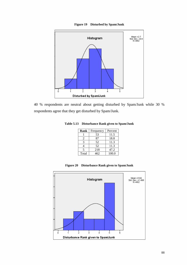
Figure 19 Disturbed by Spam/Junk
40 % respondents are neutral about getting disturbed by Spam/Junk while 30 %
respondents agree that they get disturbed by Spam/Junk.
Table 5.13 Disturbance Rank given to Spam/Junk
Figure 20 Disturbance Rank given to Spam/Junk
Rank Frequency Percent1 53 11.52 87 18.83 52 11.34 52 11.35 218 47.2
Total 462 100.0
89
Respondents are asked to rank spam, catalogs, calls, and SMS on 1 to 5 scale, where 1
means the most disturbing and 5 means the least disturbing communication. Majority
(47 %) respondents have ranked Spam/Junk fifth in a five-point disturbance rating
scale. 11 % respondents have ranked it 1st, 18 % have ranked it 2nd, 11 % have ranked
it 3rd, and 11 % have ranked it 4th.
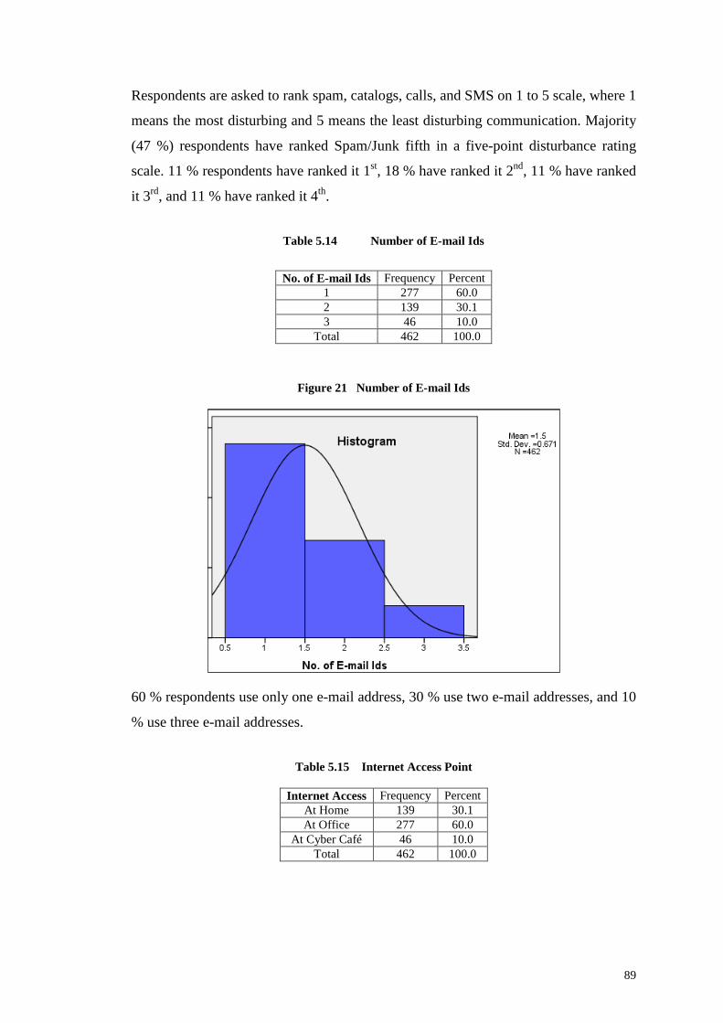
Table 5.14 Number of E-mail Ids
Figure 21 Number of E-mail Ids
60 % respondents use only one e-mail address, 30 % use two e-mail addresses, and 10
% use three e-mail addresses.
Table 5.15 Internet Access Point
No. of E-mail Ids Frequency Percent1 277 60.02 139 30.13 46 10.0
Total 462 100.0
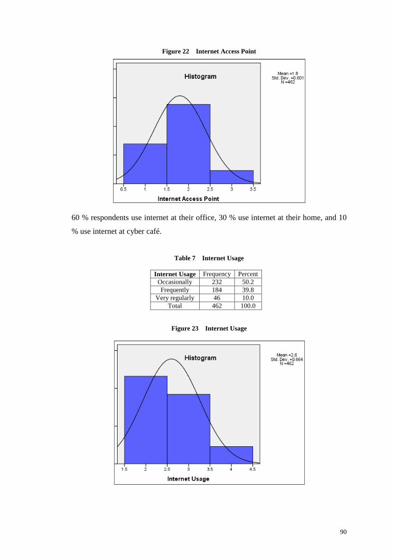
Internet Access Frequency PercentAt Home 139 30.1At Office 277 60.0
At Cyber Café 46 10.0Total 462 100.0
90
Figure 22 Internet Access Point
60 % respondents use internet at their office, 30 % use internet at their home, and 10
% use internet at cyber café.
Table 7 Internet Usage
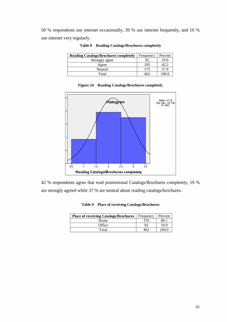
Figure 23 Internet Usage
Internet Usage Frequency PercentOccasionally 232 50.2Frequently 184 39.8
Very regularly 46 10.0Total 462 100.0
91
50 % respondents use internet occasionally, 39 % use internet frequently, and 10 %
use internet very regularly.
Table 8 Reading Catalogs/Brochures completely
Figure 24 Reading Catalogs/Brochures completely
42 % respondents agree that read promotional Catalogs/Brochures completely, 19 %
are strongly agreed while 37 % are neutral about reading catalogs/brochures.
Table 9 Place of receiving Catalogs/Brochures
Reading Catalogs/Brochures completely Frequency PercentStrongly agree 92 19.9
Agree 195 42.2Neutral 175 37.9Total 462 100.0
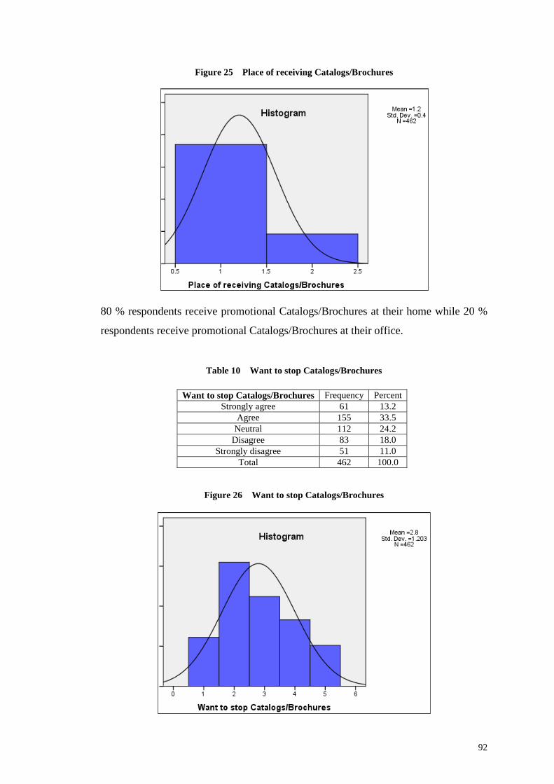
Place of receiving Catalogs/Brochures Frequency PercentHome 370 80.1Office 92 19.9Total 462 100.0
92
Figure 25 Place of receiving Catalogs/Brochures
80 % respondents receive promotional Catalogs/Brochures at their home while 20 %
respondents receive promotional Catalogs/Brochures at their office.
Table 10 Want to stop Catalogs/Brochures
Figure 26 Want to stop Catalogs/Brochures
Want to stop Catalogs/Brochures Frequency PercentStrongly agree 61 13.2
Agree 155 33.5Neutral 112 24.2
Disagree 83 18.0Strongly disagree 51 11.0
Total 462 100.0
93
Majority (33 %) respondents are agreed and 13 % respondents are strongly agreed
that they want to stop receiving unwanted Catalogs/Brochures through Direct mail.
24% are neutral while 11% strongly disagree about preferring to stop
Catalogs/Brochures.
Table 11 Thinking Catalogs/Brochures should be banned
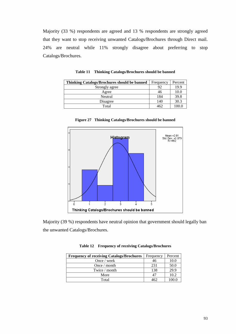
Figure 27 Thinking Catalogs/Brochures should be banned
Majority (39 %) respondents have neutral opinion that government should legally ban
the unwanted Catalogs/Brochures.
Table 12 Frequency of receiving Catalogs/Brochures
Thinking Catalogs/Brochures should be banned Frequency PercentStrongly agree 92 19.9
Agree 46 10.0Neutral 184 39.8
Disagree 140 30.3Total 462 100.0
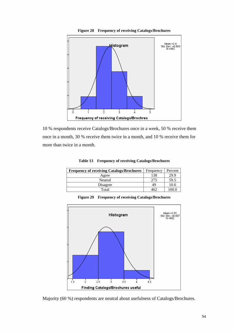
Frequency of receiving Catalogs/Brochures Frequency PercentOnce / week 46 10.0Once / month 231 50.0Twice / month 138 29.9
More 47 10.2Total 462 100.0
94
Figure 28 Frequency of receiving Catalogs/Brochures
10 % respondents receive Catalogs/Brochures once in a week, 50 % receive them
once in a month, 30 % receive them twice in a month, and 10 % receive them for
more than twice in a month.
Table 13 Frequency of receiving Catalogs/Brochures
Figure 29 Frequency of receiving Catalogs/Brochures
Majority (60 %) respondents are neutral about usefulness of Catalogs/Brochures.
Frequency of receiving Catalogs/Brochures Frequency PercentAgree 138 29.9
Neutral 275 59.5Disagree 49 10.6
Total 462 100.0
95
Table 14 Finding Catalogs/Brochures interesting
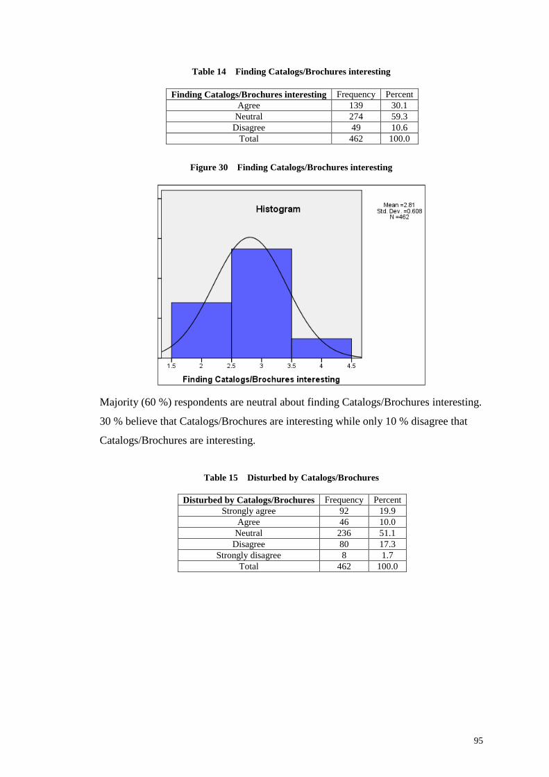
Figure 30 Finding Catalogs/Brochures interesting
Majority (60 %) respondents are neutral about finding Catalogs/Brochures interesting.
30 % believe that Catalogs/Brochures are interesting while only 10 % disagree that
Catalogs/Brochures are interesting.
Table 15 Disturbed by Catalogs/Brochures
Finding Catalogs/Brochures interesting Frequency PercentAgree 139 30.1
Neutral 274 59.3Disagree 49 10.6
Total 462 100.0
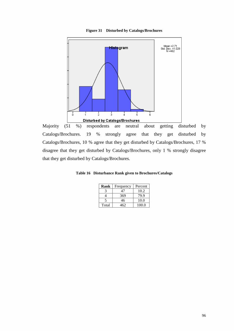
Disturbed by Catalogs/Brochures Frequency PercentStrongly agree 92 19.9
Agree 46 10.0Neutral 236 51.1
Disagree 80 17.3Strongly disagree 8 1.7
Total 462 100.0
96
Figure 31 Disturbed by Catalogs/Brochures
Majority (51 %) respondents are neutral about getting disturbed by
Catalogs/Brochures. 19 % strongly agree that they get disturbed by
Catalogs/Brochures, 10 % agree that they get disturbed by Catalogs/Brochures, 17 %
disagree that they get disturbed by Catalogs/Brochures, only 1 % strongly disagree
that they get disturbed by Catalogs/Brochures.
Table 16 Disturbance Rank given to Brochures/Catalogs
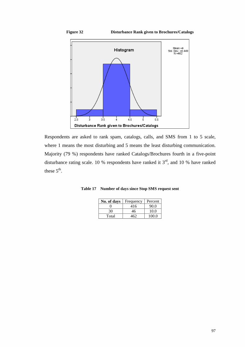
Rank Frequency Percent3 47 10.24 369 79.95 46 10.0
Total 462 100.0
97
Figure 32 Disturbance Rank given to Brochures/Catalogs
Respondents are asked to rank spam, catalogs, calls, and SMS from 1 to 5 scale,
where 1 means the most disturbing and 5 means the least disturbing communication.
Majority (79 %) respondents have ranked Catalogs/Brochures fourth in a five-point
disturbance rating scale. 10 % respondents have ranked it 3rd, and 10 % have ranked
these 5th.
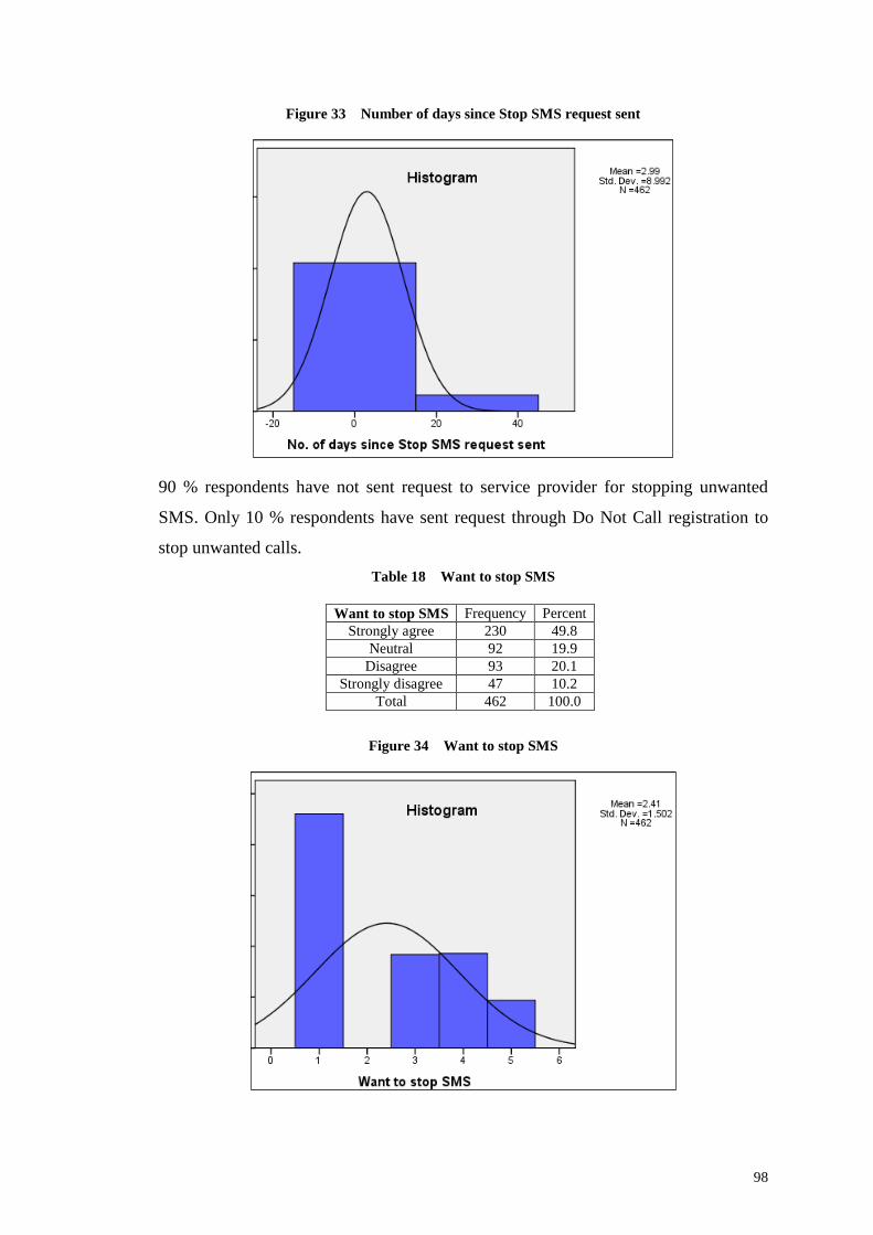
Table 17 Number of days since Stop SMS request sent
No. of days Frequency Percent0 416 90.0
30 46 10.0Total 462 100.0
98
Figure 33 Number of days since Stop SMS request sent
90 % respondents have not sent request to service provider for stopping unwanted
SMS. Only 10 % respondents have sent request through Do Not Call registration to
stop unwanted calls.
Table 18 Want to stop SMS
Figure 34 Want to stop SMS
Want to stop SMS Frequency PercentStrongly agree 230 49.8
Neutral 92 19.9Disagree 93 20.1
Strongly disagree 47 10.2Total 462 100.0
99
Majority (49 %) respondents are strongly agreed that they want to stop receiving
unwanted SMS. 19 % are neutral about this, 20 % disagree, and only 10 % strongly
disagree to prefer to stop receiving marketing SMS.
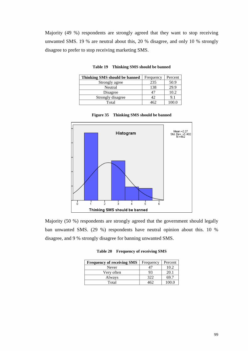
Table 19 Thinking SMS should be banned
Figure 35 Thinking SMS should be banned
Majority (50 %) respondents are strongly agreed that the government should legally
ban unwanted SMS. (29 %) respondents have neutral opinion about this. 10 %
disagree, and 9 % strongly disagree for banning unwanted SMS.
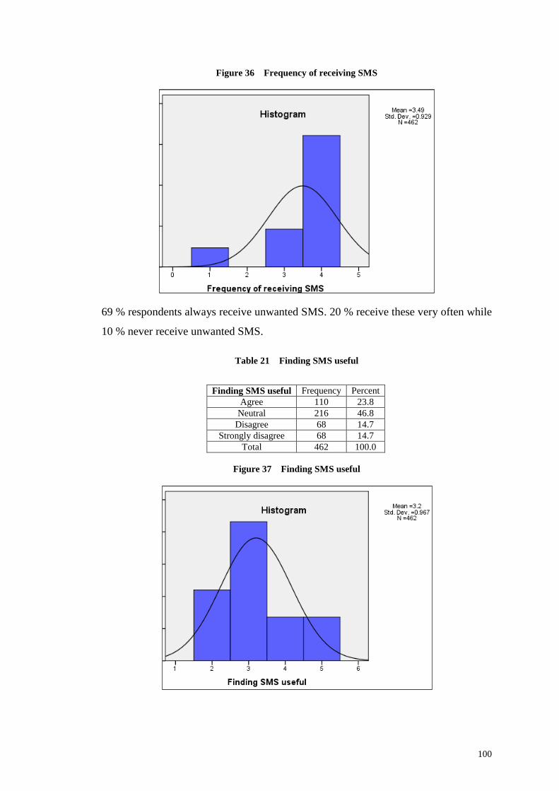
Table 20 Frequency of receiving SMS
Thinking SMS should be banned Frequency PercentStrongly agree 235 50.9
Neutral 138 29.9Disagree 47 10.2
Strongly disagree 42 9.1Total 462 100.0
Frequency of receiving SMS Frequency PercentNever 47 10.2
Very often 93 20.1Always 322 69.7Total 462 100.0
100
Figure 36 Frequency of receiving SMS
69 % respondents always receive unwanted SMS. 20 % receive these very often while
10 % never receive unwanted SMS.
Table 21 Finding SMS useful
Figure 37 Finding SMS useful
Finding SMS useful Frequency PercentAgree 110 23.8
Neutral 216 46.8Disagree 68 14.7
Strongly disagree 68 14.7Total 462 100.0
101
Majority (46 %) respondents are neutral about usefulness of unwanted SMS. 23 %
respondents agree, 14 % disagree, and 14 % strongly disagree that unwanted SMS are
useful.
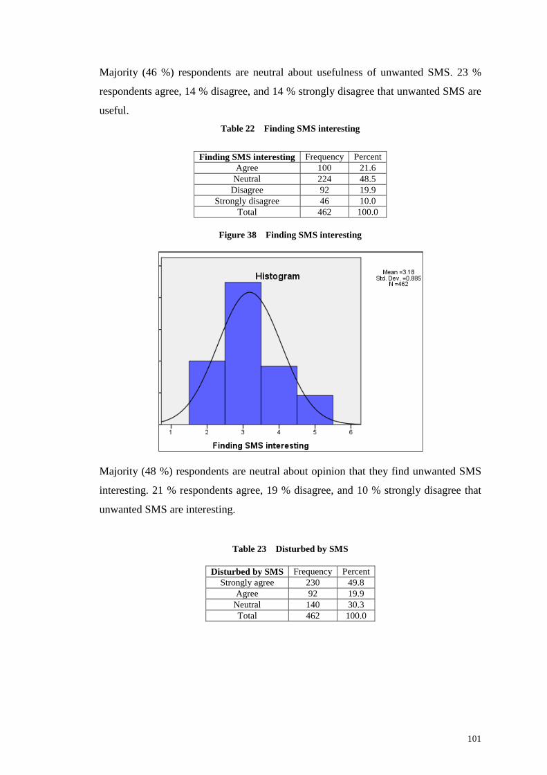
Table 22 Finding SMS interesting
Figure 38 Finding SMS interesting
Majority (48 %) respondents are neutral about opinion that they find unwanted SMS
interesting. 21 % respondents agree, 19 % disagree, and 10 % strongly disagree that
unwanted SMS are interesting.
Table 23 Disturbed by SMS
Finding SMS interesting Frequency PercentAgree 100 21.6
Neutral 224 48.5Disagree 92 19.9
Strongly disagree 46 10.0Total 462 100.0
Disturbed by SMS Frequency PercentStrongly agree 230 49.8
Agree 92 19.9Neutral 140 30.3Total 462 100.0
102
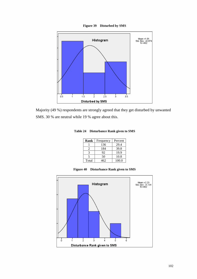
Figure 39 Disturbed by SMS
Majority (49 %) respondents are strongly agreed that they get disturbed by unwanted
SMS. 30 % are neutral while 19 % agree about this.
Table 24 Disturbance Rank given to SMS
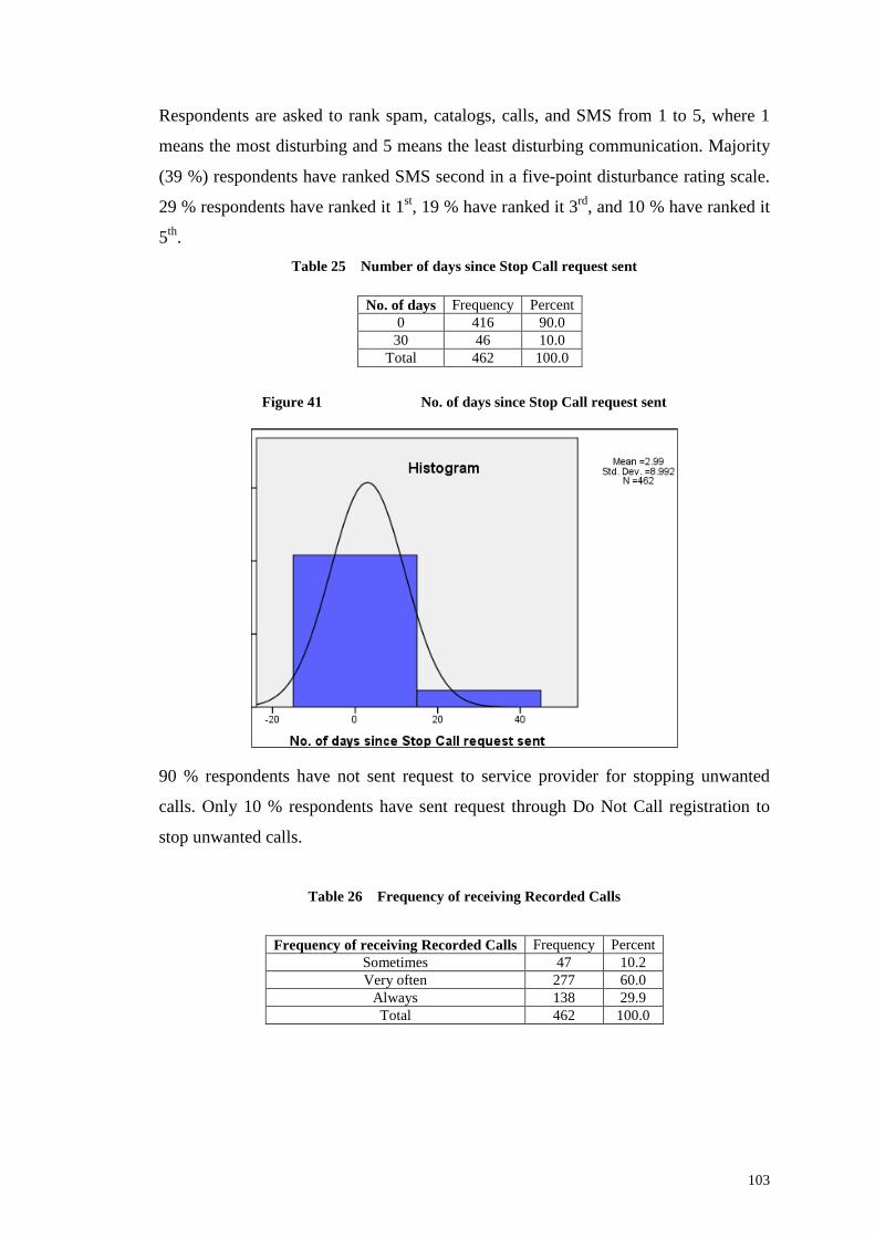
Figure 40 Disturbance Rank given to SMS
Rank Frequency Percent1 136 29.42 184 39.83 92 19.95 50 10.8
Total 462 100.0
103
Respondents are asked to rank spam, catalogs, calls, and SMS from 1 to 5, where 1
means the most disturbing and 5 means the least disturbing communication. Majority
(39 %) respondents have ranked SMS second in a five-point disturbance rating scale.
29 % respondents have ranked it 1st, 19 % have ranked it 3rd, and 10 % have ranked it
5th.
Table 25 Number of days since Stop Call request sent
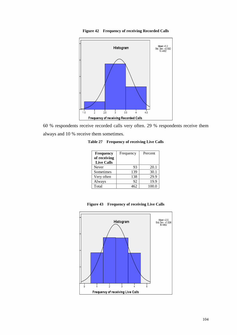
Figure 41 No. of days since Stop Call request sent
90 % respondents have not sent request to service provider for stopping unwanted
calls. Only 10 % respondents have sent request through Do Not Call registration to
stop unwanted calls.
Table 26 Frequency of receiving Recorded Calls
No. of days Frequency Percent0 416 90.0
30 46 10.0Total 462 100.0
Frequency of receiving Recorded Calls Frequency PercentSometimes 47 10.2Very often 277 60.0
Always 138 29.9Total 462 100.0
104
Figure 42 Frequency of receiving Recorded Calls
60 % respondents receive recorded calls very often. 29 % respondents receive them
always and 10 % receive them sometimes.
Table 27 Frequency of receiving Live Calls
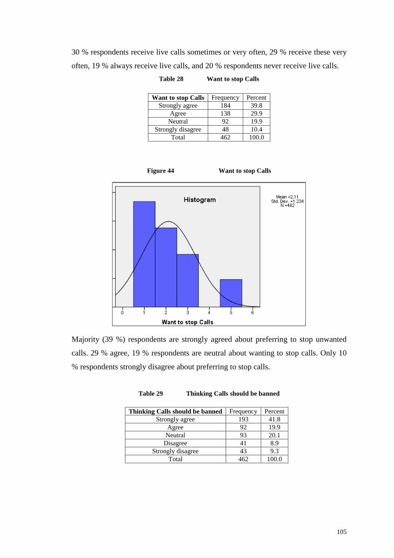
Figure 43 Frequency of receiving Live Calls
Frequencyof receivingLive Calls
Frequency Percent
Never 93 20.1Sometimes 139 30.1Very often 138 29.9Always 92 19.9Total 462 100.0
105
30 % respondents receive live calls sometimes or very often, 29 % receive these very
often, 19 % always receive live calls, and 20 % respondents never receive live calls.
Table 28 Want to stop Calls
Figure 44 Want to stop Calls
Majority (39 %) respondents are strongly agreed about preferring to stop unwanted
calls. 29 % agree, 19 % respondents are neutral about wanting to stop calls. Only 10
% respondents strongly disagree about preferring to stop calls.
Table 29 Thinking Calls should be banned
Want to stop Calls Frequency PercentStrongly agree 184 39.8
Agree 138 29.9Neutral 92 19.9
Strongly disagree 48 10.4Total 462 100.0
Thinking Calls should be banned Frequency PercentStrongly agree 193 41.8
Agree 92 19.9Neutral 93 20.1
Disagree 41 8.9Strongly disagree 43 9.3
Total 462 100.0
106
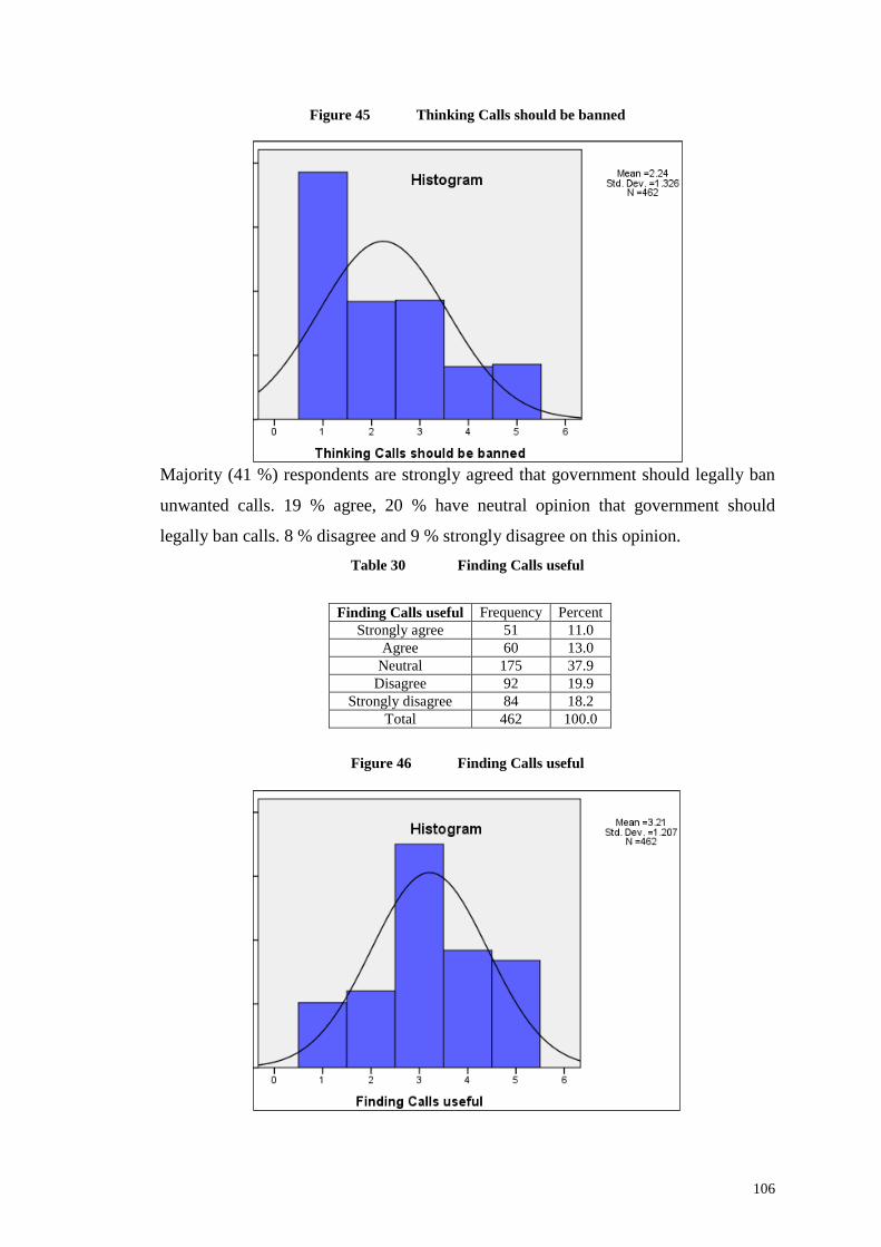
Figure 45 Thinking Calls should be banned
Majority (41 %) respondents are strongly agreed that government should legally ban
unwanted calls. 19 % agree, 20 % have neutral opinion that government should
legally ban calls. 8 % disagree and 9 % strongly disagree on this opinion.
Table 30 Finding Calls useful
Figure 46 Finding Calls useful
Finding Calls useful Frequency PercentStrongly agree 51 11.0
Agree 60 13.0Neutral 175 37.9
Disagree 92 19.9Strongly disagree 84 18.2
Total 462 100.0
107
Majority (37 %) respondents are neutral about usefulness of unwanted calls. 11 %
strongly agree, 13 % agree, 19 % disagree, and 18 %strongly disagree about finding
calls useful.
Table 31 Finding Calls interesting
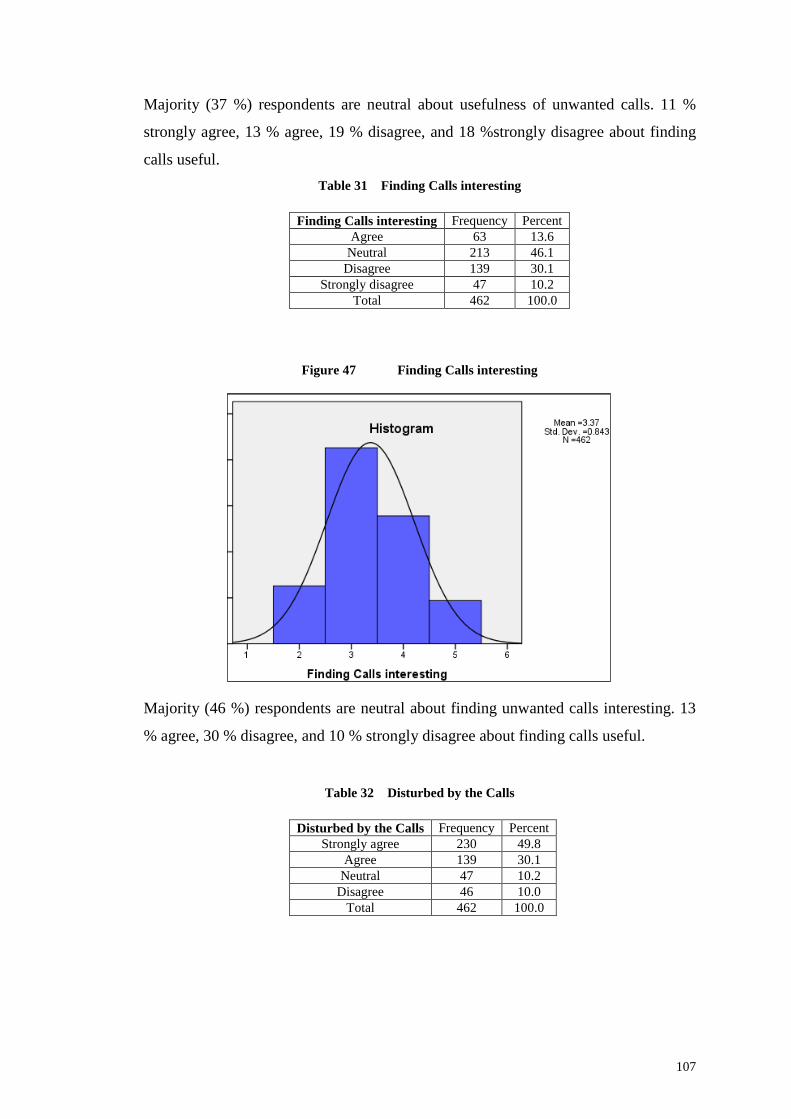
Figure 47 Finding Calls interesting
Majority (46 %) respondents are neutral about finding unwanted calls interesting. 13
% agree, 30 % disagree, and 10 % strongly disagree about finding calls useful.
Table 32 Disturbed by the Calls
Finding Calls interesting Frequency PercentAgree 63 13.6
Neutral 213 46.1Disagree 139 30.1
Strongly disagree 47 10.2Total 462 100.0
Disturbed by the Calls Frequency PercentStrongly agree 230 49.8
Agree 139 30.1Neutral 47 10.2
Disagree 46 10.0Total 462 100.0
108
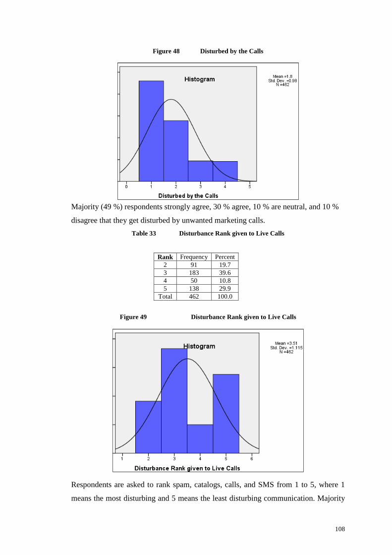
Figure 48 Disturbed by the Calls
Majority (49 %) respondents strongly agree, 30 % agree, 10 % are neutral, and 10 %
disagree that they get disturbed by unwanted marketing calls.
Table 33 Disturbance Rank given to Live Calls
Figure 49 Disturbance Rank given to Live Calls
Respondents are asked to rank spam, catalogs, calls, and SMS from 1 to 5, where 1
means the most disturbing and 5 means the least disturbing communication. Majority
Rank Frequency Percent2 91 19.73 183 39.64 50 10.85 138 29.9
Total 462 100.0
109
(39 %) respondents have ranked live calls third in a five-point disturbance rating
scale. No respondent has ranked it 1st, 19 % have ranked it 2nd, 10 % have ranked it
4th, and 29 % have ranked it 5th.
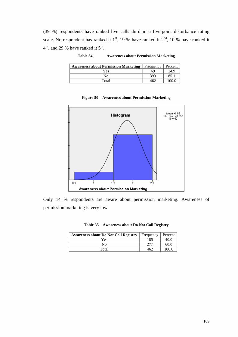
Table 34 Awareness about Permission Marketing
Figure 50 Awareness about Permission Marketing
Only 14 % respondents are aware about permission marketing. Awareness of
permission marketing is very low.
Table 35 Awareness about Do Not Call Registry
Awareness about Permission Marketing Frequency PercentYes 69 14.9No 393 85.1
Total 462 100.0
Awareness about Do Not Call Registry Frequency PercentYes 185 40.0No 277 60.0
Total 462 100.0
110
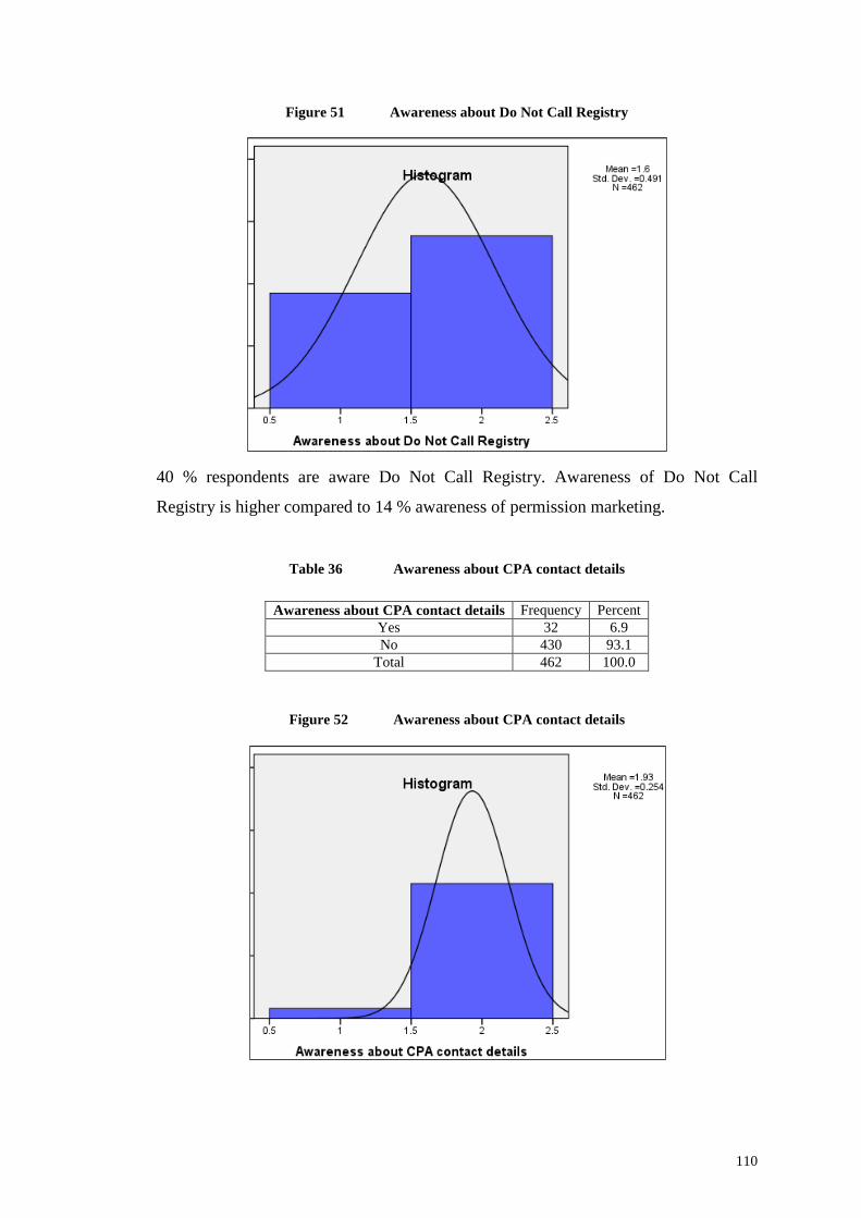
Figure 51 Awareness about Do Not Call Registry
40 % respondents are aware Do Not Call Registry. Awareness of Do Not Call
Registry is higher compared to 14 % awareness of permission marketing.
Table 36 Awareness about CPA contact details
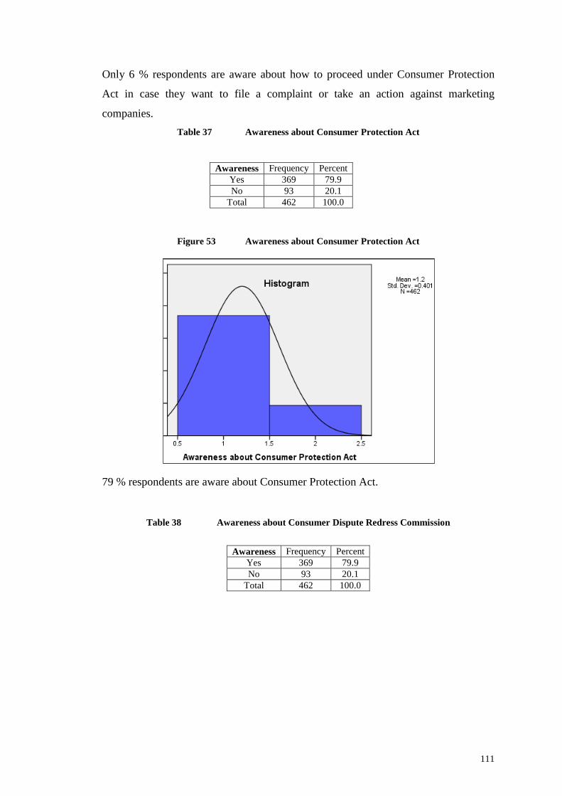
Figure 52 Awareness about CPA contact details
Awareness about CPA contact details Frequency PercentYes 32 6.9No 430 93.1
Total 462 100.0
111
Only 6 % respondents are aware about how to proceed under Consumer Protection
Act in case they want to file a complaint or take an action against marketing
companies.
Table 37 Awareness about Consumer Protection Act
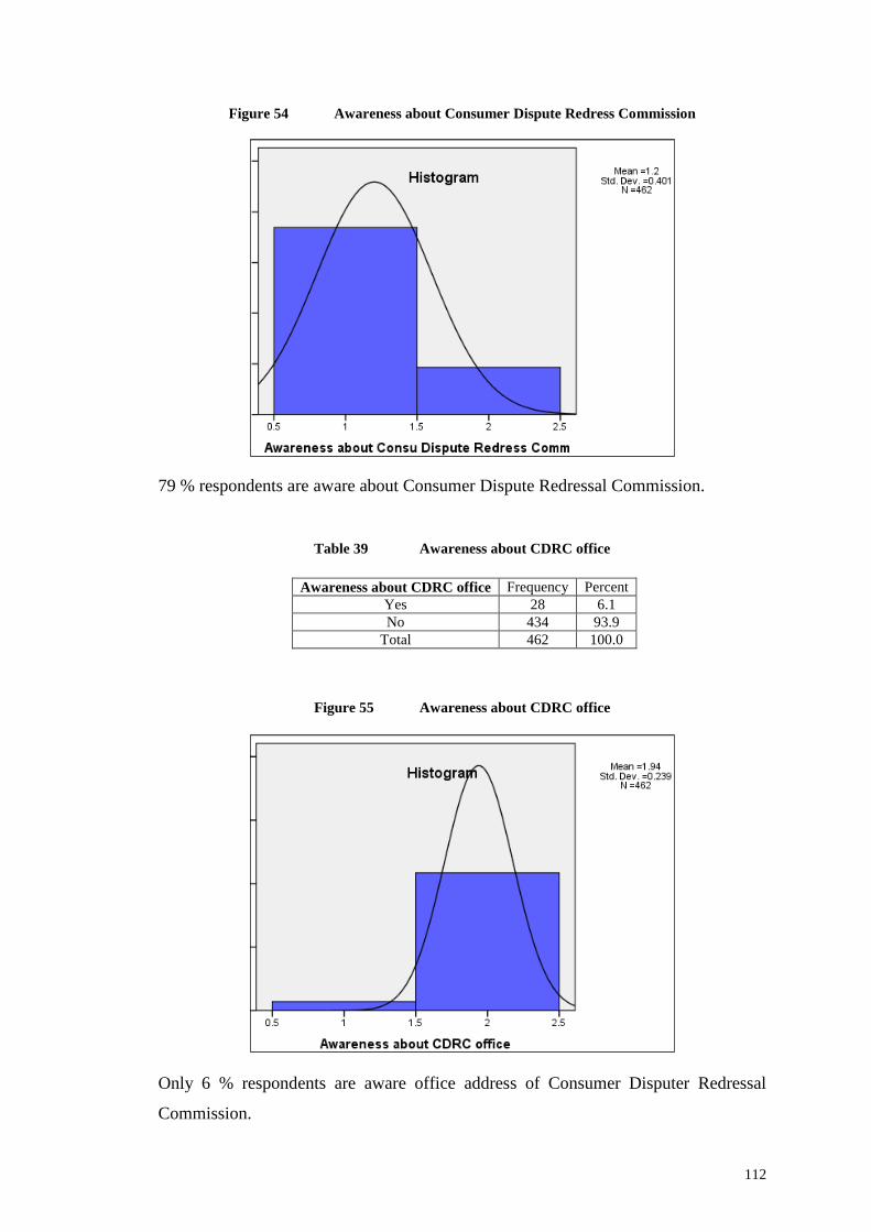
Figure 53 Awareness about Consumer Protection Act
79 % respondents are aware about Consumer Protection Act.
Table 38 Awareness about Consumer Dispute Redress Commission
Awareness Frequency PercentYes 369 79.9No 93 20.1
Total 462 100.0
Awareness Frequency PercentYes 369 79.9No 93 20.1
Total 462 100.0
112
Figure 54 Awareness about Consumer Dispute Redress Commission
79 % respondents are aware about Consumer Dispute Redressal Commission.
Table 39 Awareness about CDRC office
Figure 55 Awareness about CDRC office
Only 6 % respondents are aware office address of Consumer Disputer Redressal
Commission.
Awareness about CDRC office Frequency PercentYes 28 6.1No 434 93.9
Total 462 100.0
113
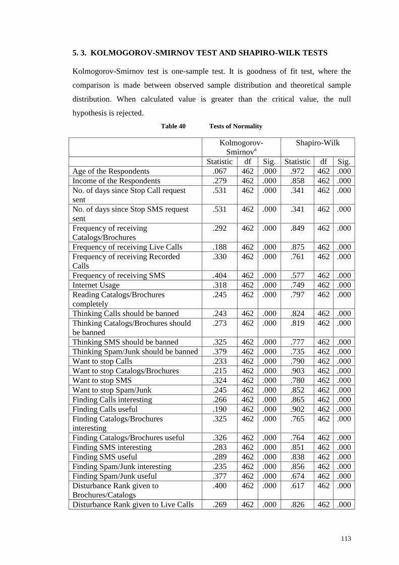
5. 3. KOLMOGOROV-SMIRNOV TEST AND SHAPIRO-WILK TESTS
Kolmogorov-Smirnov test is one-sample test. It is goodness of fit test, where the
comparison is made between observed sample distribution and theoretical sample
distribution. When calculated value is greater than the critical value, the null
hypothesis is rejected.
Table 40 Tests of Normality
Kolmogorov-Smirnova
Shapiro-Wilk
Statistic df Sig. Statistic df Sig.Age of the Respondents .067 462 .000 .972 462 .000Income of the Respondents .279 462 .000 .858 462 .000No. of days since Stop Call requestsent
.531 462 .000 .341 462 .000
No. of days since Stop SMS requestsent
.531 462 .000 .341 462 .000
Frequency of receivingCatalogs/Brochures
.292 462 .000 .849 462 .000
Frequency of receiving Live Calls .188 462 .000 .875 462 .000Frequency of receiving RecordedCalls
.330 462 .000 .761 462 .000
Frequency of receiving SMS .404 462 .000 .577 462 .000Internet Usage .318 462 .000 .749 462 .000Reading Catalogs/Brochurescompletely
.245 462 .000 .797 462 .000
Thinking Calls should be banned .243 462 .000 .824 462 .000Thinking Catalogs/Brochures shouldbe banned
.273 462 .000 .819 462 .000
Thinking SMS should be banned .325 462 .000 .777 462 .000Thinking Spam/Junk should be banned .379 462 .000 .735 462 .000Want to stop Calls .233 462 .000 .790 462 .000Want to stop Catalogs/Brochures .215 462 .000 .903 462 .000Want to stop SMS .324 462 .000 .780 462 .000Want to stop Spam/Junk .245 462 .000 .852 462 .000Finding Calls interesting .266 462 .000 .865 462 .000Finding Calls useful .190 462 .000 .902 462 .000Finding Catalogs/Brochuresinteresting
.325 462 .000 .765 462 .000
Finding Catalogs/Brochures useful .326 462 .000 .764 462 .000Finding SMS interesting .283 462 .000 .851 462 .000Finding SMS useful .289 462 .000 .838 462 .000Finding Spam/Junk interesting .235 462 .000 .856 462 .000Finding Spam/Junk useful .377 462 .000 .674 462 .000Disturbance Rank given toBrochures/Catalogs
.400 462 .000 .617 462 .000
Disturbance Rank given to Live Calls .269 462 .000 .826 462 .000
114
Disturbance Rank given to RecordedCalls
.372 462 .000 .695 462 .000
Disturbance Rank given to SMS .269 462 .000 .806 462 .000Disturbance Rank given to Spam/Junk .290 462 .000 .791 462 .000Disturbed by Catalogs/Brochures .312 462 .000 .839 462 .000Disturbed by SMS .319 462 .000 .734 462 .000Disturbed by Spam/Junk .231 462 .000 .875 462 .000Disturbed by the Calls .291 462 .000 .762 462 .000City of the Respondents .147 462 .000 .905 462 .000Education of the Respondents .190 462 .000 .874 462 .000Gender of the Respondents .436 462 .000 .584 462 .000Internet Access Point .330 462 .000 .760 462 .000No. of E-mail Ids .372 462 .000 .702 462 .000Occupation of the Respondents .170 462 .000 .873 462 .000Place of receiving Catalogs/Brochures .492 462 .000 .489 462 .000Treatment with Spam/Junk .442 462 .000 .577 462 .000Awareness about Consumer ProtectionAct
.491 462 .000 .491 462 .000
Awareness about CPA contact details .538 462 .000 .275 462 .000Awareness about Do Not CallRegistry
.392 462 .000 .622 462 .000
Awareness about PermissionMarketing
.513 462 .000 .425 462 .000
City of the Respondents .147 462 .000 .905 462 .000a. Lilliefors Significance Correction
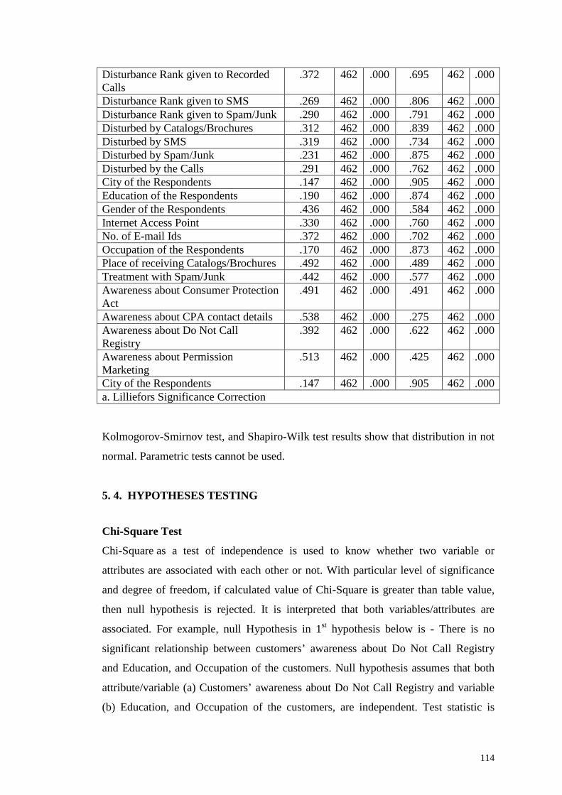
Kolmogorov-Smirnov test, and Shapiro-Wilk test results show that distribution in not
normal. Parametric tests cannot be used.
5. 4. HYPOTHESES TESTING
Chi-Square Test
Chi-Square as a test of independence is used to know whether two variable or
attributes are associated with each other or not. With particular level of significance
and degree of freedom, if calculated value of Chi-Square is greater than table value,
then null hypothesis is rejected. It is interpreted that both variables/attributes are
associated. For example, null Hypothesis in 1st hypothesis below is - There is no
significant relationship between customers’ awareness about Do Not Call Registry
and Education, and Occupation of the customers. Null hypothesis assumes that both
attribute/variable (a) Customers’ awareness about Do Not Call Registry and variable
(b) Education, and Occupation of the customers, are independent. Test statistic is
115
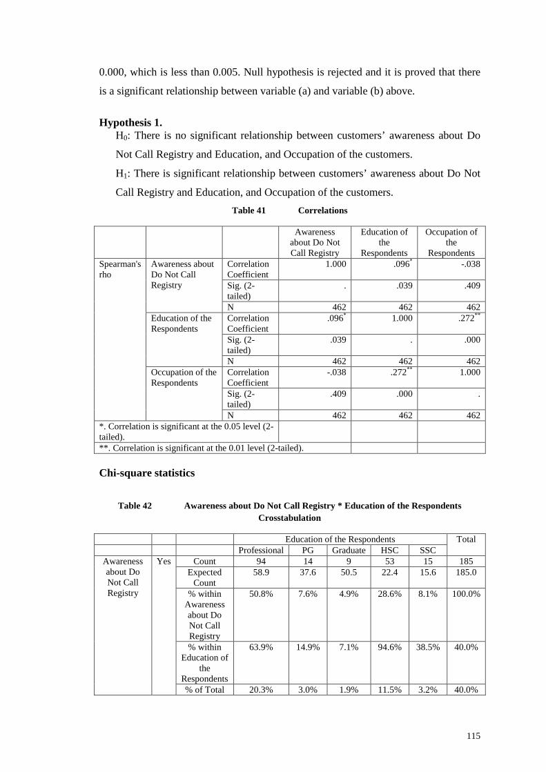
0.000, which is less than 0.005. Null hypothesis is rejected and it is proved that there
is a significant relationship between variable (a) and variable (b) above.
Hypothesis 1.H0: There is no significant relationship between customers’ awareness about Do
Not Call Registry and Education, and Occupation of the customers.
H1: There is significant relationship between customers’ awareness about Do Not
Call Registry and Education, and Occupation of the customers.
Table 41 Correlations
Awarenessabout Do NotCall Registry
Education ofthe
Respondents
Occupation ofthe
RespondentsSpearman'srho
Awareness aboutDo Not CallRegistry
CorrelationCoefficient
1.000 .096* -.038
Sig. (2-tailed)
. .039 .409
N 462 462 462Education of theRespondents
CorrelationCoefficient
.096* 1.000 .272**
Sig. (2-tailed)
.039 . .000
N 462 462 462Occupation of theRespondents
CorrelationCoefficient
-.038 .272** 1.000
Sig. (2-tailed)
.409 .000 .
N 462 462 462*. Correlation is significant at the 0.05 level (2-tailed).**. Correlation is significant at the 0.01 level (2-tailed).
Chi-square statistics
Table 42 Awareness about Do Not Call Registry * Education of the Respondents
Crosstabulation
Education of the Respondents TotalProfessional PG Graduate HSC SSC
Awarenessabout DoNot CallRegistry
Yes Count 94 14 9 53 15 185Expected
Count58.9 37.6 50.5 22.4 15.6 185.0
% withinAwarenessabout DoNot CallRegistry
50.8% 7.6% 4.9% 28.6% 8.1% 100.0%
% withinEducation of
theRespondents
63.9% 14.9% 7.1% 94.6% 38.5% 40.0%
% of Total 20.3% 3.0% 1.9% 11.5% 3.2% 40.0%
116
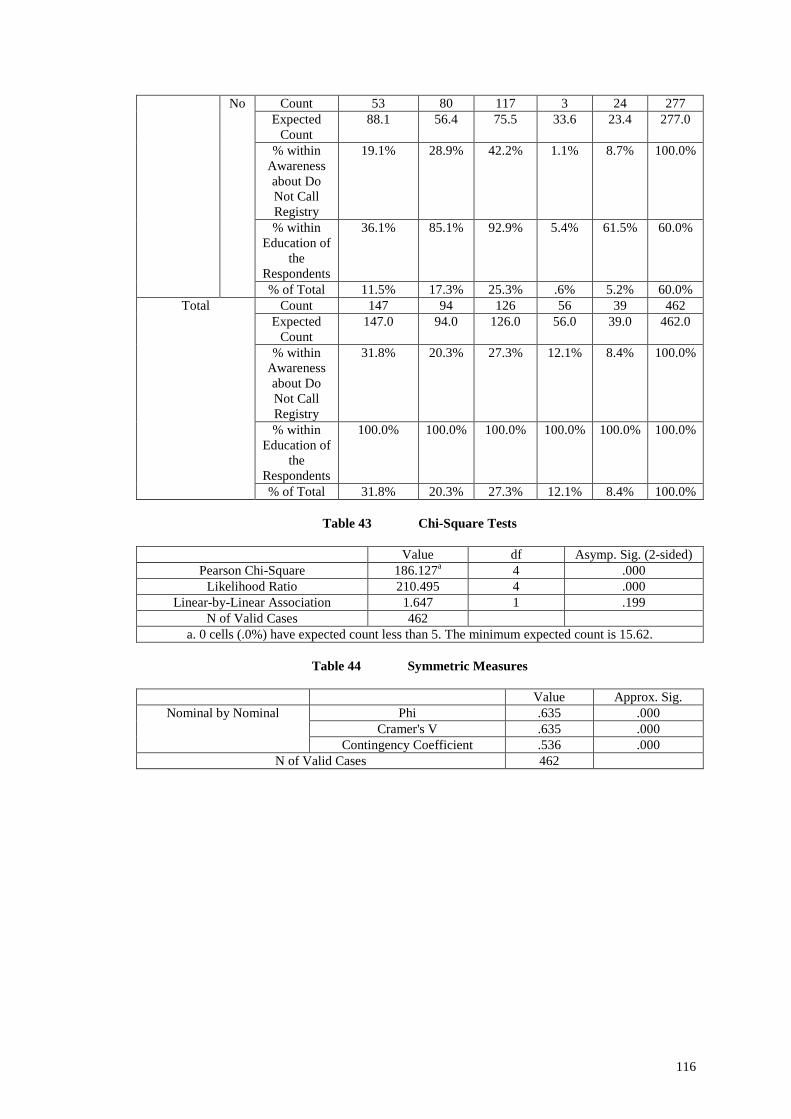
No Count 53 80 117 3 24 277Expected
Count88.1 56.4 75.5 33.6 23.4 277.0
% withinAwarenessabout DoNot CallRegistry
19.1% 28.9% 42.2% 1.1% 8.7% 100.0%
% withinEducation of
theRespondents
36.1% 85.1% 92.9% 5.4% 61.5% 60.0%
% of Total 11.5% 17.3% 25.3% .6% 5.2% 60.0%Total Count 147 94 126 56 39 462
ExpectedCount
147.0 94.0 126.0 56.0 39.0 462.0
% withinAwarenessabout DoNot CallRegistry
31.8% 20.3% 27.3% 12.1% 8.4% 100.0%
% withinEducation of
theRespondents
100.0% 100.0% 100.0% 100.0% 100.0% 100.0%
% of Total 31.8% 20.3% 27.3% 12.1% 8.4% 100.0%
Table 43 Chi-Square Tests
Value df Asymp. Sig. (2-sided)Pearson Chi-Square 186.127a 4 .000
Likelihood Ratio 210.495 4 .000Linear-by-Linear Association 1.647 1 .199
N of Valid Cases 462a. 0 cells (.0%) have expected count less than 5. The minimum expected count is 15.62.
Table 44 Symmetric Measures
Value Approx. Sig.Nominal by Nominal Phi .635 .000
Cramer's V .635 .000Contingency Coefficient .536 .000
N of Valid Cases 462
117
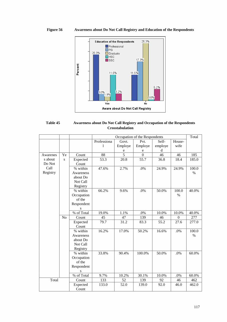
Figure 56 Awareness about Do Not Call Registry and Education of the Respondents
Table 45 Awareness about Do Not Call Registry and Occupation of the Respondents
Crosstabulation
Occupation of the Respondents TotalProfessiona
lGovt.
Employee
Pvt.Employe
e
Self-employe
d
House-wife
Awareness aboutDo Not
CallRegistry
Yes
Count 88 5 0 46 46 185Expected
Count53.3 20.8 55.7 36.8 18.4 185.0
% withinAwarenessabout DoNot CallRegistry
47.6% 2.7% .0% 24.9% 24.9% 100.0%
% withinOccupation
of theRespondent
s
66.2% 9.6% .0% 50.0% 100.0%
40.0%
% of Total 19.0% 1.1% .0% 10.0% 10.0% 40.0%No Count 45 47 139 46 0 277
ExpectedCount
79.7 31.2 83.3 55.2 27.6 277.0
% withinAwarenessabout DoNot CallRegistry
16.2% 17.0% 50.2% 16.6% .0% 100.0%
% withinOccupation
of theRespondent
s
33.8% 90.4% 100.0% 50.0% .0% 60.0%
% of Total 9.7% 10.2% 30.1% 10.0% .0% 60.0%Total Count 133 52 139 92 46 462
ExpectedCount
133.0 52.0 139.0 92.0 46.0 462.0
118
% withinAwarenessabout DoNot CallRegistry
28.8% 11.3% 30.1% 19.9% 10.0% 100.0%
% withinOccupation
of theRespondent
s
100.0% 100.0% 100.0% 100.0% 100.0%
100.0%
% of Total 28.8% 11.3% 30.1% 19.9% 10.0% 100.0%
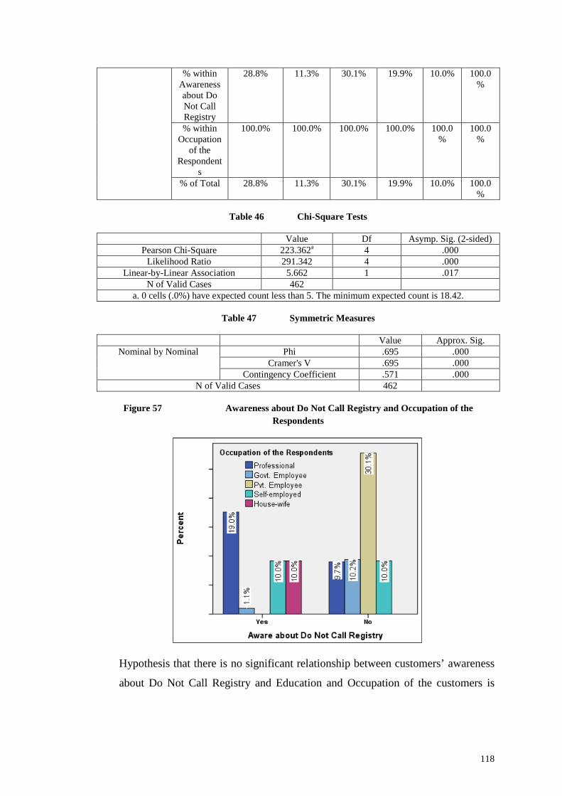
Table 46 Chi-Square Tests
Value Df Asymp. Sig. (2-sided)Pearson Chi-Square 223.362a 4 .000
Likelihood Ratio 291.342 4 .000Linear-by-Linear Association 5.662 1 .017
N of Valid Cases 462a. 0 cells (.0%) have expected count less than 5. The minimum expected count is 18.42.
Table 47 Symmetric Measures
Value Approx. Sig.Nominal by Nominal Phi .695 .000
Cramer's V .695 .000Contingency Coefficient .571 .000
N of Valid Cases 462
Figure 57 Awareness about Do Not Call Registry and Occupation of the
Respondents
Hypothesis that there is no significant relationship between customers’ awareness
about Do Not Call Registry and Education and Occupation of the customers is
119
rejected. There is significant relationship between customers’ awareness about Do
Not Call Registry and customers’ education and occupation.
Hypothesis 2.
H0: There is no significant relationship between customers’ awareness about Do
Not Call Registry and City, and Gender of the customers.
H1: There is significant relationship between customers’ awareness about Do Not
Call Registry and City, and Gender of the customers.
Table 48 Correlations
Awarenessabout DoNot CallRegistry
City of theRespondents
Gender ofthe
Respondents
Spearman'srho
Awareness about DoNot Call Registry
CorrelationCoefficient
1.000 .012 -.048
Sig. (2-tailed) . .802 .301N 462 462 462
City of theRespondents
CorrelationCoefficient
.012 1.000 .053
Sig. (2-tailed) .802 . .257N 462 462 462
Gender of theRespondents
CorrelationCoefficient
-.048 .053 1.000
Sig. (2-tailed) .301 .257 .N 462 462 462
Chi-square statistics
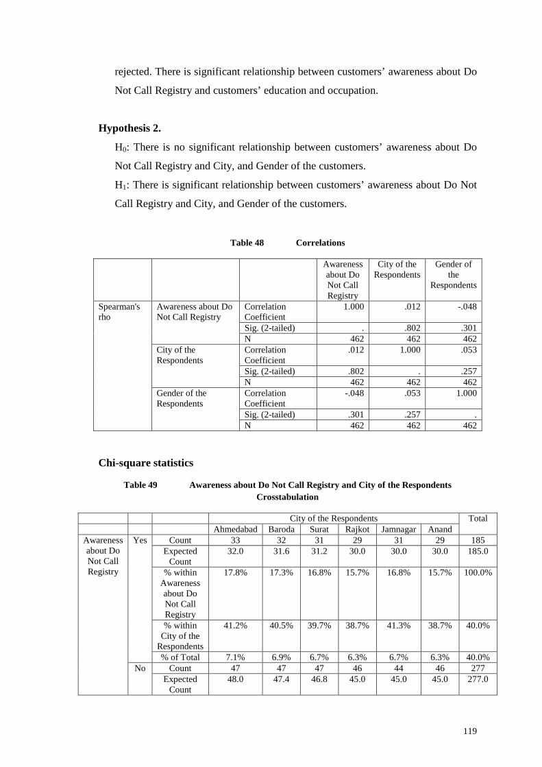
Table 49 Awareness about Do Not Call Registry and City of the Respondents
Crosstabulation
City of the Respondents TotalAhmedabad Baroda Surat Rajkot Jamnagar Anand
Awarenessabout DoNot CallRegistry
Yes Count 33 32 31 29 31 29 185Expected
Count32.0 31.6 31.2 30.0 30.0 30.0 185.0
% withinAwarenessabout DoNot CallRegistry
17.8% 17.3% 16.8% 15.7% 16.8% 15.7% 100.0%
% withinCity of the
Respondents
41.2% 40.5% 39.7% 38.7% 41.3% 38.7% 40.0%
% of Total 7.1% 6.9% 6.7% 6.3% 6.7% 6.3% 40.0%No Count 47 47 47 46 44 46 277
ExpectedCount
48.0 47.4 46.8 45.0 45.0 45.0 277.0
120
% withinAwarenessabout DoNot CallRegistry
17.0% 17.0% 17.0% 16.6% 15.9% 16.6% 100.0%
% withinCity of the
Respondents
58.8% 59.5% 60.3% 61.3% 58.7% 61.3% 60.0%
% of Total 10.2% 10.2% 10.2% 10.0% 9.5% 10.0% 60.0%Total Count 80 79 78 75 75 75 462
ExpectedCount
80.0 79.0 78.0 75.0 75.0 75.0 462.0
% withinAwarenessabout DoNot CallRegistry
17.3% 17.1% 16.9% 16.2% 16.2% 16.2% 100.0%
% withinCity of the
Respondents
100.0% 100.0% 100.0% 100.0% 100.0% 100.0% 100.0%
% of Total 17.3% 17.1% 16.9% 16.2% 16.2% 16.2% 100.0%
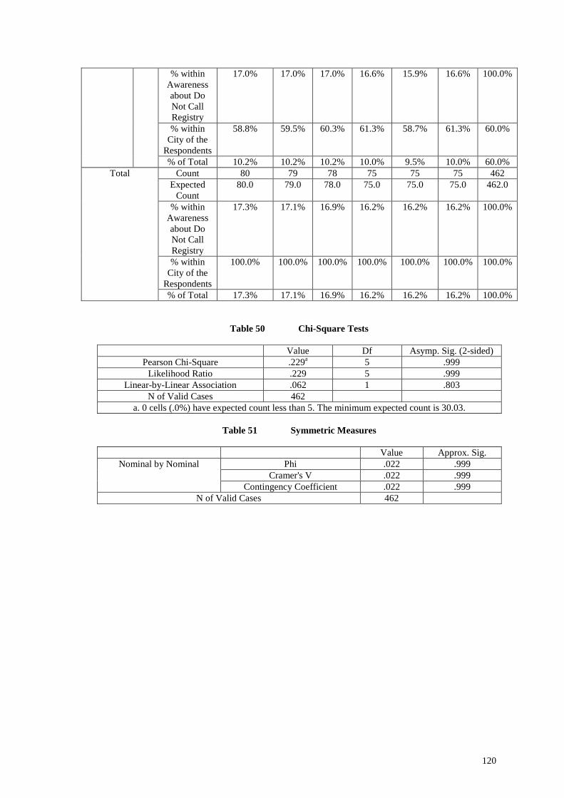
Table 50 Chi-Square Tests
Value Df Asymp. Sig. (2-sided)Pearson Chi-Square .229a 5 .999
Likelihood Ratio .229 5 .999Linear-by-Linear Association .062 1 .803
N of Valid Cases 462a. 0 cells (.0%) have expected count less than 5. The minimum expected count is 30.03.
Table 51 Symmetric Measures
Value Approx. Sig.Nominal by Nominal Phi .022 .999
Cramer's V .022 .999Contingency Coefficient .022 .999
N of Valid Cases 462
121
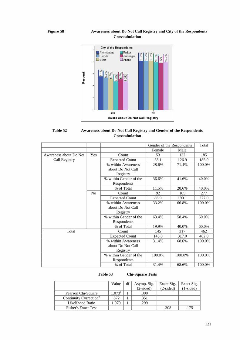
Figure 58 Awareness about Do Not Call Registry and City of the Respondents
Crosstabulation
Table 52 Awareness about Do Not Call Registry and Gender of the Respondents
Crosstabulation
Gender of the Respondents TotalFemale Male
Awareness about Do NotCall Registry
Yes Count 53 132 185Expected Count 58.1 126.9 185.0
% within Awarenessabout Do Not Call
Registry
28.6% 71.4% 100.0%
% within Gender of theRespondents
36.6% 41.6% 40.0%
% of Total 11.5% 28.6% 40.0%No Count 92 185 277
Expected Count 86.9 190.1 277.0% within Awarenessabout Do Not Call
Registry
33.2% 66.8% 100.0%
% within Gender of theRespondents
63.4% 58.4% 60.0%
% of Total 19.9% 40.0% 60.0%Total Count 145 317 462
Expected Count 145.0 317.0 462.0% within Awarenessabout Do Not Call
Registry
31.4% 68.6% 100.0%
% within Gender of theRespondents
100.0% 100.0% 100.0%
% of Total 31.4% 68.6% 100.0%
Table 53 Chi-Square Tests
Value df Asymp. Sig.(2-sided)
Exact Sig.(2-sided)
Exact Sig.(1-sided)
Pearson Chi-Square 1.073a 1 .300Continuity Correctionb .872 1 .351
Likelihood Ratio 1.079 1 .299Fisher's Exact Test .308 .175
122
Linear-by-Linear Association 1.071 1 .301N of Valid Casesb 462
a. 0 cells (.0%) have expected count less than 5. The minimum expected count is 58.06.b. Computed only for a 2x2 table
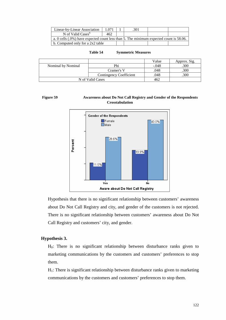
Table 54 Symmetric Measures
Value Approx. Sig.Nominal by Nominal Phi -.048 .300
Cramer's V .048 .300Contingency Coefficient .048 .300
N of Valid Cases 462
Figure 59 Awareness about Do Not Call Registry and Gender of the Respondents
Crosstabulation
Hypothesis that there is no significant relationship between customers’ awareness
about Do Not Call Registry and city, and gender of the customers is not rejected.
There is no significant relationship between customers’ awareness about Do Not
Call Registry and customers’ city, and gender.
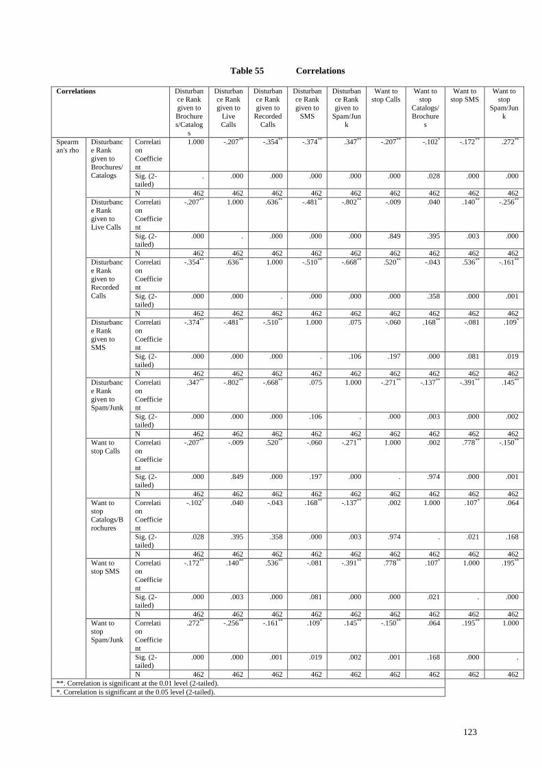
Hypothesis 3.
H0: There is no significant relationship between disturbance ranks given to
marketing communications by the customers and customers’ preferences to stop
them.
H1: There is significant relationship between disturbance ranks given to marketing
communications by the customers and customers’ preferences to stop them.
123
Table 55 Correlations
Correlations Disturbance Rankgiven toBrochures/Catalog
s
Disturbance Rankgiven to
LiveCalls
Disturbance Rankgiven to
RecordedCalls
Disturbance Rankgiven to
SMS
Disturbance Rankgiven to
Spam/Junk
Want tostop Calls
Want tostop
Catalogs/Brochure
s
Want tostop SMS
Want tostop
Spam/Junk
Spearman's rho
Disturbance Rankgiven toBrochures/Catalogs
CorrelationCoefficient
1.000 -.207** -.354** -.374** .347** -.207** -.102* -.172** .272**
Sig. (2-tailed)
. .000 .000 .000 .000 .000 .028 .000 .000
N 462 462 462 462 462 462 462 462 462Disturbance Rankgiven toLive Calls
CorrelationCoefficient
-.207** 1.000 .636** -.481** -.802** -.009 .040 .140** -.256**
Sig. (2-tailed)
.000 . .000 .000 .000 .849 .395 .003 .000
N 462 462 462 462 462 462 462 462 462Disturbance Rankgiven toRecordedCalls
CorrelationCoefficient
-.354** .636** 1.000 -.510** -.668** .520** -.043 .536** -.161**
Sig. (2-tailed)
.000 .000 . .000 .000 .000 .358 .000 .001
N 462 462 462 462 462 462 462 462 462Disturbance Rankgiven toSMS
CorrelationCoefficient
-.374** -.481** -.510** 1.000 .075 -.060 .168** -.081 .109*
Sig. (2-tailed)
.000 .000 .000 . .106 .197 .000 .081 .019
N 462 462 462 462 462 462 462 462 462Disturbance Rankgiven toSpam/Junk
CorrelationCoefficient
.347** -.802** -.668** .075 1.000 -.271** -.137** -.391** .145**
Sig. (2-tailed)
.000 .000 .000 .106 . .000 .003 .000 .002
N 462 462 462 462 462 462 462 462 462Want tostop Calls
CorrelationCoefficient
-.207** -.009 .520** -.060 -.271** 1.000 .002 .778** -.150**
Sig. (2-tailed)
.000 .849 .000 .197 .000 . .974 .000 .001
N 462 462 462 462 462 462 462 462 462Want tostopCatalogs/Brochures
CorrelationCoefficient
-.102* .040 -.043 .168** -.137** .002 1.000 .107* .064
Sig. (2-tailed)
.028 .395 .358 .000 .003 .974 . .021 .168
N 462 462 462 462 462 462 462 462 462Want tostop SMS
CorrelationCoefficient
-.172** .140** .536** -.081 -.391** .778** .107* 1.000 .195**
Sig. (2-tailed)
.000 .003 .000 .081 .000 .000 .021 . .000
N 462 462 462 462 462 462 462 462 462Want tostopSpam/Junk
CorrelationCoefficient
.272** -.256** -.161** .109* .145** -.150** .064 .195** 1.000
Sig. (2-tailed)
.000 .000 .001 .019 .002 .001 .168 .000 .
N 462 462 462 462 462 462 462 462 462**. Correlation is significant at the 0.01 level (2-tailed).*. Correlation is significant at the 0.05 level (2-tailed).
124
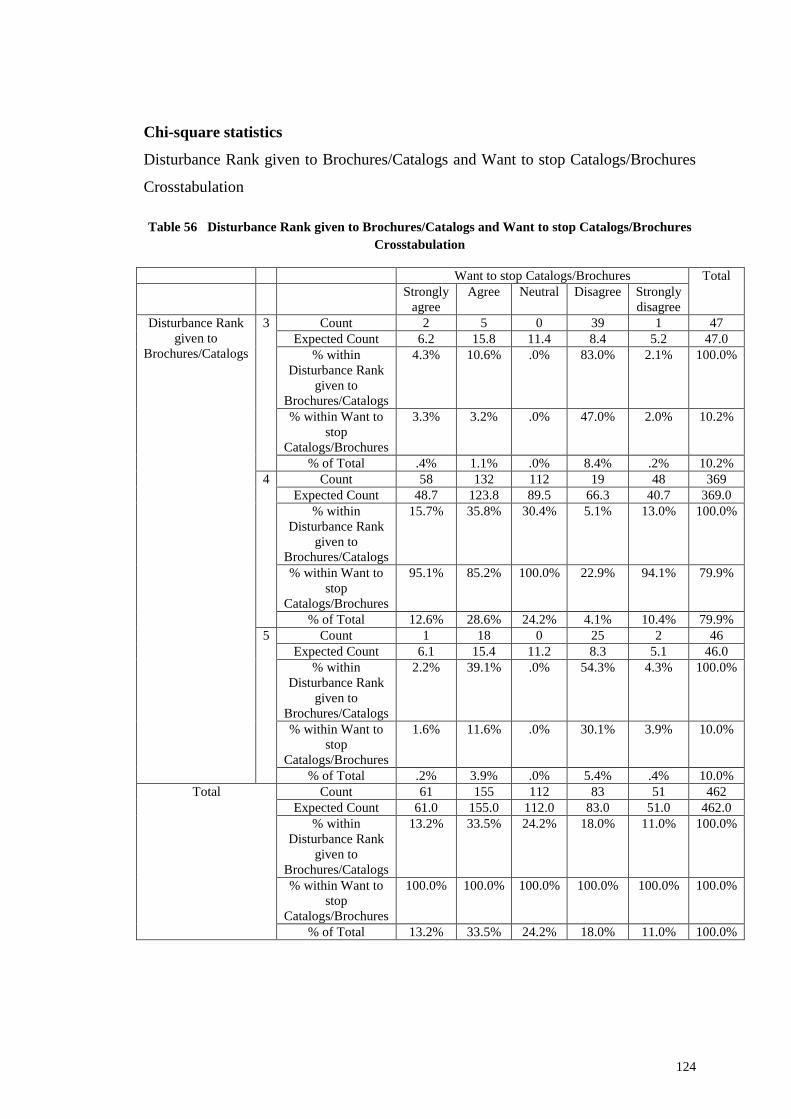
Chi-square statistics
Disturbance Rank given to Brochures/Catalogs and Want to stop Catalogs/Brochures
Crosstabulation
Table 56 Disturbance Rank given to Brochures/Catalogs and Want to stop Catalogs/Brochures
Crosstabulation
Want to stop Catalogs/Brochures TotalStrongly
agreeAgree Neutral Disagree Strongly
disagreeDisturbance Rank
given toBrochures/Catalogs
3 Count 2 5 0 39 1 47Expected Count 6.2 15.8 11.4 8.4 5.2 47.0
% withinDisturbance Rank
given toBrochures/Catalogs
4.3% 10.6% .0% 83.0% 2.1% 100.0%
% within Want tostop
Catalogs/Brochures
3.3% 3.2% .0% 47.0% 2.0% 10.2%
% of Total .4% 1.1% .0% 8.4% .2% 10.2%4 Count 58 132 112 19 48 369
Expected Count 48.7 123.8 89.5 66.3 40.7 369.0% within
Disturbance Rankgiven to
Brochures/Catalogs
15.7% 35.8% 30.4% 5.1% 13.0% 100.0%
% within Want tostop
Catalogs/Brochures
95.1% 85.2% 100.0% 22.9% 94.1% 79.9%
% of Total 12.6% 28.6% 24.2% 4.1% 10.4% 79.9%5 Count 1 18 0 25 2 46
Expected Count 6.1 15.4 11.2 8.3 5.1 46.0% within
Disturbance Rankgiven to
Brochures/Catalogs
2.2% 39.1% .0% 54.3% 4.3% 100.0%
% within Want tostop
Catalogs/Brochures
1.6% 11.6% .0% 30.1% 3.9% 10.0%
% of Total .2% 3.9% .0% 5.4% .4% 10.0%Total Count 61 155 112 83 51 462
Expected Count 61.0 155.0 112.0 83.0 51.0 462.0% within
Disturbance Rankgiven to
Brochures/Catalogs
13.2% 33.5% 24.2% 18.0% 11.0% 100.0%
% within Want tostop
Catalogs/Brochures
100.0% 100.0% 100.0% 100.0% 100.0% 100.0%
% of Total 13.2% 33.5% 24.2% 18.0% 11.0% 100.0%
125
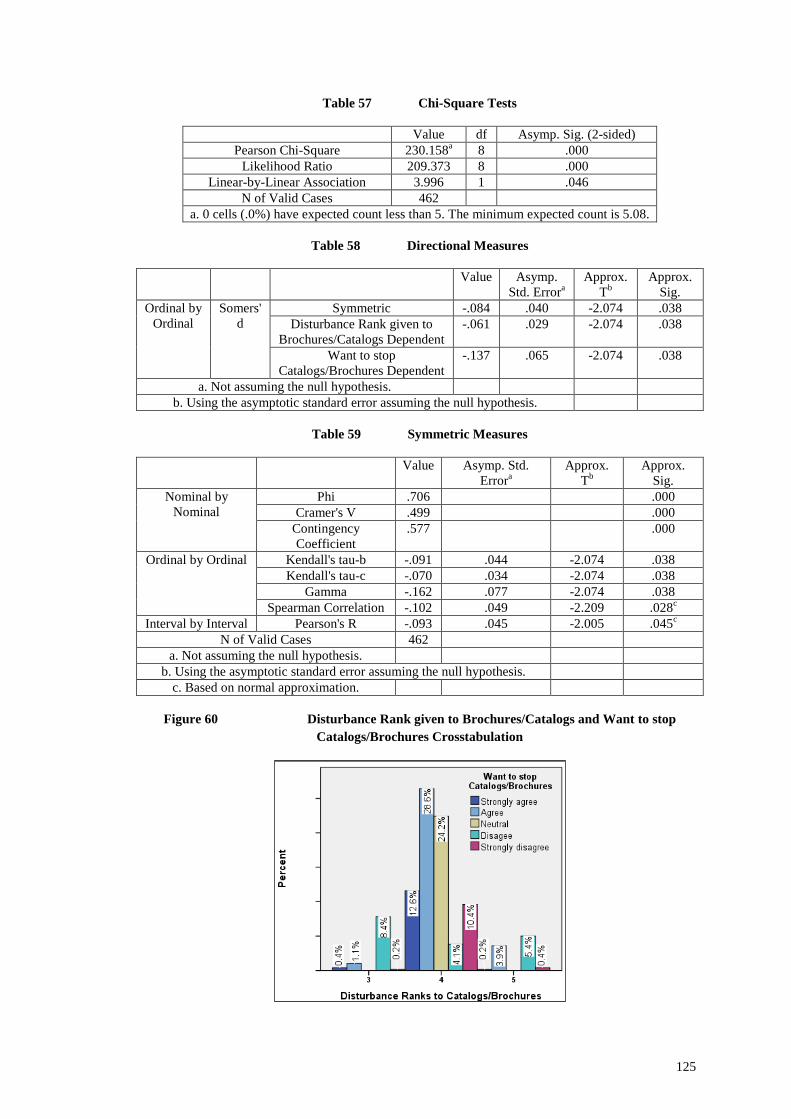
Table 57 Chi-Square Tests
Value df Asymp. Sig. (2-sided)Pearson Chi-Square 230.158a 8 .000
Likelihood Ratio 209.373 8 .000Linear-by-Linear Association 3.996 1 .046
N of Valid Cases 462a. 0 cells (.0%) have expected count less than 5. The minimum expected count is 5.08.
Table 58 Directional Measures
Value Asymp.Std. Errora
Approx.Tb
Approx.Sig.
Ordinal byOrdinal
Somers'd
Symmetric -.084 .040 -2.074 .038Disturbance Rank given to
Brochures/Catalogs Dependent-.061 .029 -2.074 .038
Want to stopCatalogs/Brochures Dependent
-.137 .065 -2.074 .038
a. Not assuming the null hypothesis.b. Using the asymptotic standard error assuming the null hypothesis.
Table 59 Symmetric Measures
Value Asymp. Std.Errora
Approx.Tb
Approx.Sig.
Nominal byNominal
Phi .706 .000Cramer's V .499 .000
ContingencyCoefficient
.577 .000
Ordinal by Ordinal Kendall's tau-b -.091 .044 -2.074 .038Kendall's tau-c -.070 .034 -2.074 .038
Gamma -.162 .077 -2.074 .038Spearman Correlation -.102 .049 -2.209 .028c
Interval by Interval Pearson's R -.093 .045 -2.005 .045c
N of Valid Cases 462a. Not assuming the null hypothesis.
b. Using the asymptotic standard error assuming the null hypothesis.c. Based on normal approximation.
Figure 60 Disturbance Rank given to Brochures/Catalogs and Want to stop
Catalogs/Brochures Crosstabulation
126
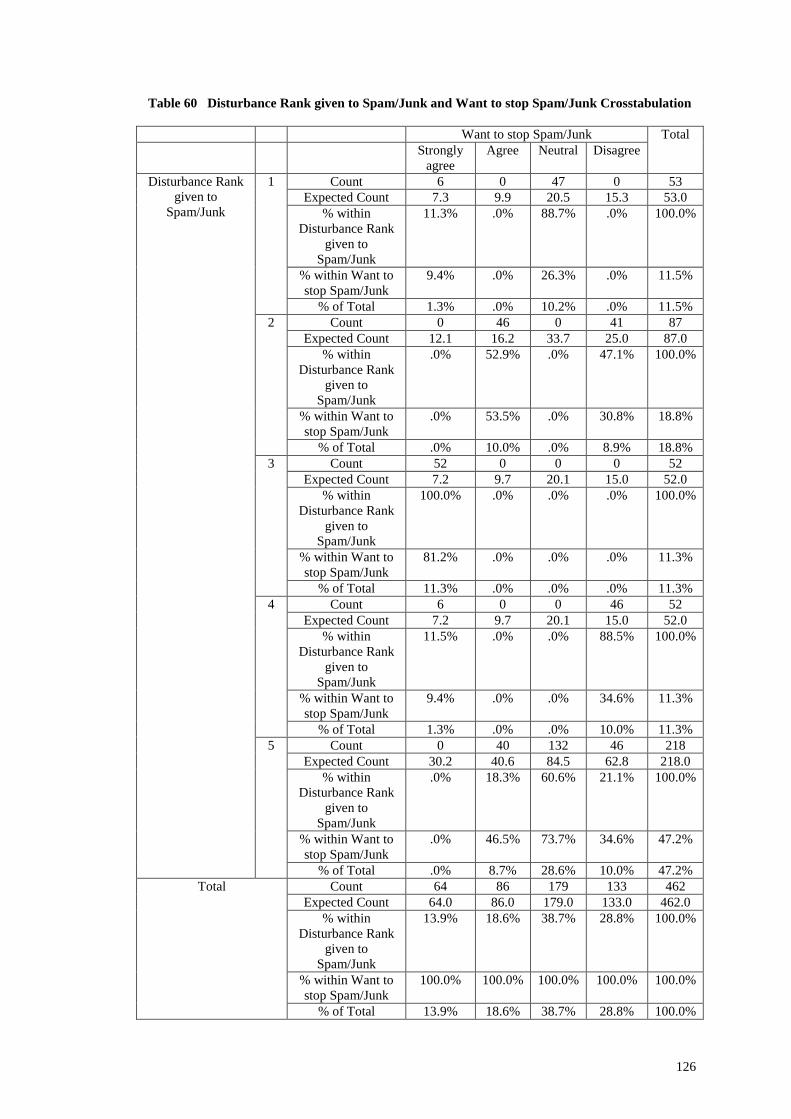
Table 60 Disturbance Rank given to Spam/Junk and Want to stop Spam/Junk Crosstabulation
Want to stop Spam/Junk TotalStrongly
agreeAgree Neutral Disagree
Disturbance Rankgiven to
Spam/Junk
1 Count 6 0 47 0 53Expected Count 7.3 9.9 20.5 15.3 53.0
% withinDisturbance Rank
given toSpam/Junk
11.3% .0% 88.7% .0% 100.0%
% within Want tostop Spam/Junk
9.4% .0% 26.3% .0% 11.5%
% of Total 1.3% .0% 10.2% .0% 11.5%2 Count 0 46 0 41 87
Expected Count 12.1 16.2 33.7 25.0 87.0% within
Disturbance Rankgiven to
Spam/Junk
.0% 52.9% .0% 47.1% 100.0%
% within Want tostop Spam/Junk
.0% 53.5% .0% 30.8% 18.8%
% of Total .0% 10.0% .0% 8.9% 18.8%3 Count 52 0 0 0 52
Expected Count 7.2 9.7 20.1 15.0 52.0% within
Disturbance Rankgiven to
Spam/Junk
100.0% .0% .0% .0% 100.0%
% within Want tostop Spam/Junk
81.2% .0% .0% .0% 11.3%
% of Total 11.3% .0% .0% .0% 11.3%4 Count 6 0 0 46 52
Expected Count 7.2 9.7 20.1 15.0 52.0% within
Disturbance Rankgiven to
Spam/Junk
11.5% .0% .0% 88.5% 100.0%
% within Want tostop Spam/Junk
9.4% .0% .0% 34.6% 11.3%
% of Total 1.3% .0% .0% 10.0% 11.3%5 Count 0 40 132 46 218
Expected Count 30.2 40.6 84.5 62.8 218.0% within
Disturbance Rankgiven to
Spam/Junk
.0% 18.3% 60.6% 21.1% 100.0%
% within Want tostop Spam/Junk
.0% 46.5% 73.7% 34.6% 47.2%
% of Total .0% 8.7% 28.6% 10.0% 47.2%Total Count 64 86 179 133 462
Expected Count 64.0 86.0 179.0 133.0 462.0% within
Disturbance Rankgiven to
Spam/Junk
13.9% 18.6% 38.7% 28.8% 100.0%
% within Want tostop Spam/Junk
100.0% 100.0% 100.0% 100.0% 100.0%
% of Total 13.9% 18.6% 38.7% 28.8% 100.0%
127
Table 61 Chi-Square Tests
Value df Asymp. Sig. (2-sided)Pearson Chi-Square 649.416a 12 .000
Likelihood Ratio 606.676 12 .000Linear-by-Linear Association 15.527 1 .000
N of Valid Cases 462a. 0 cells (.0%) have expected count less than 5. The minimum expected count is 7.20.
Table 62 Directional Measures
Value Asymp. Std.Errora
Approx.Tb
Approx.Sig.
Ordinal byOrdinal
Somers'd
Symmetric .092 .028 3.200 .001Disturbance Rank given to
Spam/Junk Dependent.091 .028 3.200 .001
Want to stop Spam/JunkDependent
.092 .029 3.200 .001
a. Not assuming the null hypothesis.b. Using the asymptotic standard error assuming the null hypothesis.
Table 63 Symmetric Measures
Value Asymp. Std.Errora
Approx.Tb
Approx.Sig.
Nominal byNominal
Phi 1.186 .000Cramer's V .685 .000
ContingencyCoefficient
.764 .000
Ordinal by Ordinal Kendall's tau-b .092 .028 3.200 .001Kendall's tau-c .086 .027 3.200 .001
Gamma .114 .035 3.200 .001Spearman Correlation .145 .039 3.141 .002c
Interval by Interval Pearson's R .184 .035 4.004 .000c
N of Valid Cases 462a. Not assuming the null hypothesis.
b. Using the asymptotic standard error assuming the null hypothesis.c. Based on normal approximation.
Figure 61 Disturbance Rank given to Spam/Junk and Want to stop Spam/Junk
Crosstabulation
128
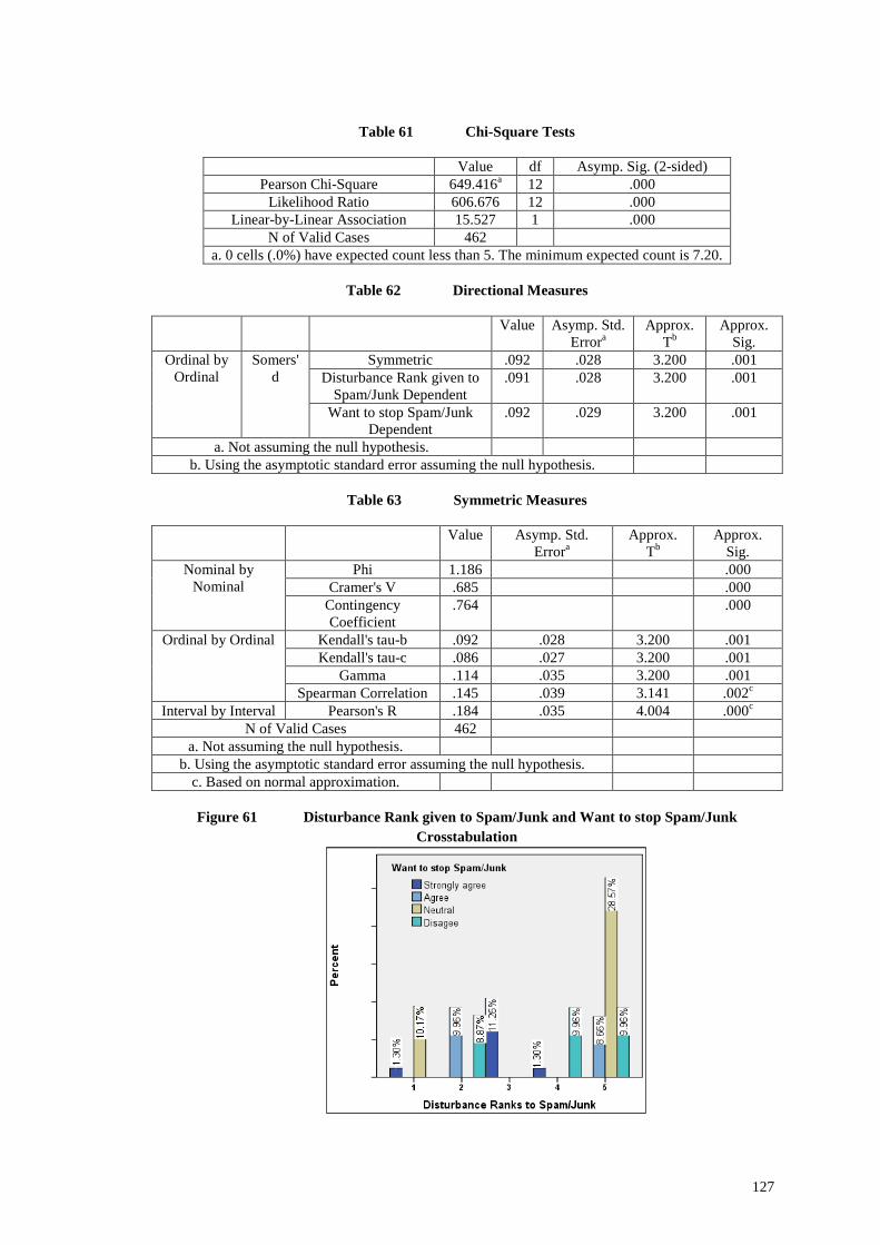
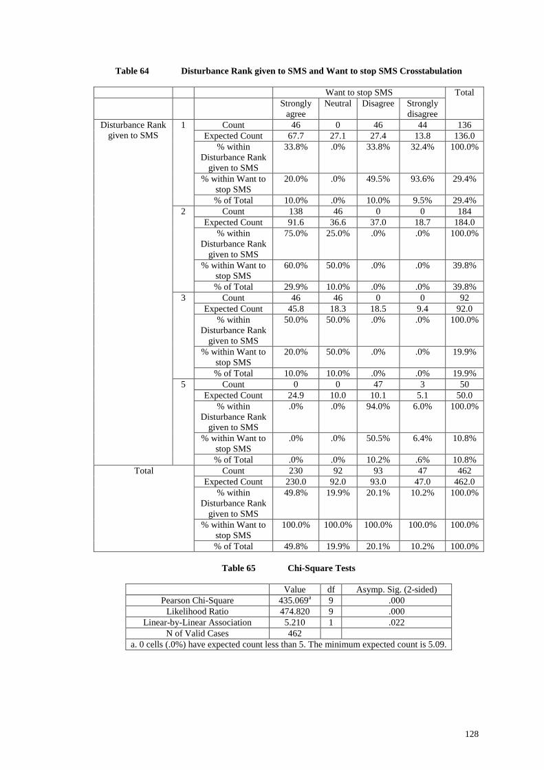
Table 64 Disturbance Rank given to SMS and Want to stop SMS Crosstabulation
Want to stop SMS TotalStrongly
agreeNeutral Disagree Strongly
disagreeDisturbance Rank
given to SMS1 Count 46 0 46 44 136
Expected Count 67.7 27.1 27.4 13.8 136.0% within
Disturbance Rankgiven to SMS
33.8% .0% 33.8% 32.4% 100.0%
% within Want tostop SMS
20.0% .0% 49.5% 93.6% 29.4%
% of Total 10.0% .0% 10.0% 9.5% 29.4%2 Count 138 46 0 0 184
Expected Count 91.6 36.6 37.0 18.7 184.0% within
Disturbance Rankgiven to SMS
75.0% 25.0% .0% .0% 100.0%
% within Want tostop SMS
60.0% 50.0% .0% .0% 39.8%
% of Total 29.9% 10.0% .0% .0% 39.8%3 Count 46 46 0 0 92
Expected Count 45.8 18.3 18.5 9.4 92.0% within
Disturbance Rankgiven to SMS
50.0% 50.0% .0% .0% 100.0%
% within Want tostop SMS
20.0% 50.0% .0% .0% 19.9%
% of Total 10.0% 10.0% .0% .0% 19.9%5 Count 0 0 47 3 50
Expected Count 24.9 10.0 10.1 5.1 50.0% within
Disturbance Rankgiven to SMS
.0% .0% 94.0% 6.0% 100.0%
% within Want tostop SMS
.0% .0% 50.5% 6.4% 10.8%
% of Total .0% .0% 10.2% .6% 10.8%Total Count 230 92 93 47 462
Expected Count 230.0 92.0 93.0 47.0 462.0% within
Disturbance Rankgiven to SMS
49.8% 19.9% 20.1% 10.2% 100.0%
% within Want tostop SMS
100.0% 100.0% 100.0% 100.0% 100.0%
% of Total 49.8% 19.9% 20.1% 10.2% 100.0%
Table 65 Chi-Square Tests
Value df Asymp. Sig. (2-sided)Pearson Chi-Square 435.069a 9 .000
Likelihood Ratio 474.820 9 .000Linear-by-Linear Association 5.210 1 .022
N of Valid Cases 462a. 0 cells (.0%) have expected count less than 5. The minimum expected count is 5.09.
129
Table 66 Directional Measures
Value Asymp. Std.Errora
Approx.Tb
Approx.Sig.
Ordinal byOrdinal
Somers'd
Symmetric -.030 .052 -.583 .560Disturbance Rank given to
SMS Dependent-.031 .053 -.583 .560
Want to stop SMSDependent
-.029 .051 -.583 .560
a. Not assuming the null hypothesis.b. Using the asymptotic standard error assuming the null hypothesis.
Table 67 Symmetric Measures
Value Asymp. Std.Errora
Approx.Tb
Approx.Sig.
Nominal byNominal
Phi .970 .000Cramer's V .560 .000
ContingencyCoefficient
.696 .000
Ordinal by Ordinal Kendall's tau-b -.030 .052 -.583 .560Kendall's tau-c -.028 .047 -.583 .560
Gamma -.040 .068 -.583 .560Spearman Correlation -.081 .059 -1.752 .081c
Interval by Interval Pearson's R .106 .051 2.293 .022c
N of Valid Cases 462a. Not assuming the null hypothesis.
b. Using the asymptotic standard error assuming the null hypothesis.c. Based on normal approximation.
Figure 62 Disturbance Rank given to SMS and Want to stop SMS Crosstabulation
Table 68 Disturbance Rank given to Recorded Calls and Want to stop Calls
Crosstabulation
Want to stop Calls TotalStrongly
agreeAgree Neutral Strongly
disagreeDisturbance Rankgiven to Recorded
Calls
1 Count 184 46 45 1 276Expected Count 109.9 82.4 55.0 28.7 276.0
% within 66.7% 16.7% 16.3% .4% 100.0%
130
Disturbance Rankgiven to Recorded
Calls% within Want to
stop Calls100.0% 33.3% 48.9% 2.1% 59.7%
% of Total 39.8% 10.0% 9.7% .2% 59.7%2 Count 0 0 47 46 93
Expected Count 37.0 27.8 18.5 9.7 93.0% within
Disturbance Rankgiven to Recorded
Calls
.0% .0% 50.5% 49.5% 100.0%
% within Want tostop Calls
.0% .0% 51.1% 95.8% 20.1%
% of Total .0% .0% 10.2% 10.0% 20.1%3 Count 0 92 0 1 93
Expected Count 37.0 27.8 18.5 9.7 93.0% within
Disturbance Rankgiven to Recorded
Calls
.0% 98.9% .0% 1.1% 100.0%
% within Want tostop Calls
.0% 66.7% .0% 2.1% 20.1%
% of Total .0% 19.9% .0% .2% 20.1%Total Count 184 138 92 48 462
Expected Count 184.0 138.0 92.0 48.0 462.0% within
Disturbance Rankgiven to Recorded
Calls
39.8% 29.9% 19.9% 10.4% 100.0%
% within Want tostop Calls
100.0% 100.0% 100.0% 100.0% 100.0%
% of Total 39.8% 29.9% 19.9% 10.4% 100.0%
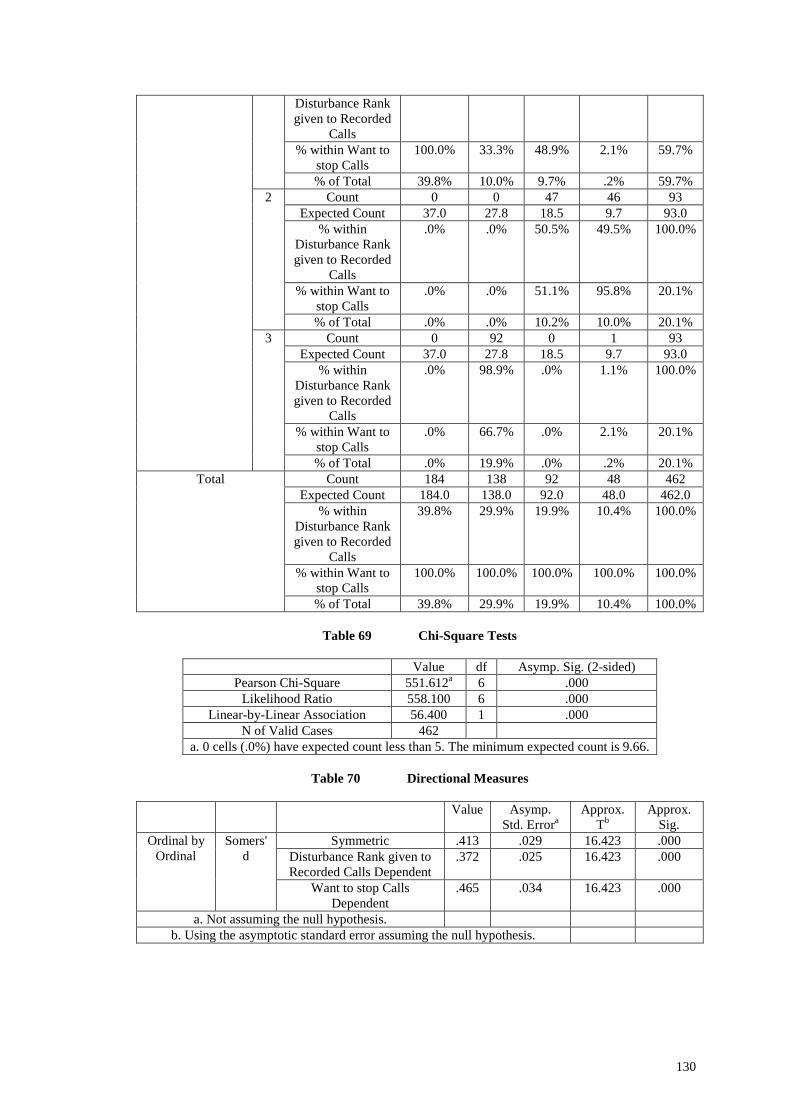
Table 69 Chi-Square Tests
Value df Asymp. Sig. (2-sided)Pearson Chi-Square 551.612a 6 .000
Likelihood Ratio 558.100 6 .000Linear-by-Linear Association 56.400 1 .000
N of Valid Cases 462a. 0 cells (.0%) have expected count less than 5. The minimum expected count is 9.66.
Table 70 Directional Measures
Value Asymp.Std. Errora
Approx.Tb
Approx.Sig.
Ordinal byOrdinal
Somers'd
Symmetric .413 .029 16.423 .000Disturbance Rank given toRecorded Calls Dependent
.372 .025 16.423 .000
Want to stop CallsDependent
.465 .034 16.423 .000
a. Not assuming the null hypothesis.b. Using the asymptotic standard error assuming the null hypothesis.
131
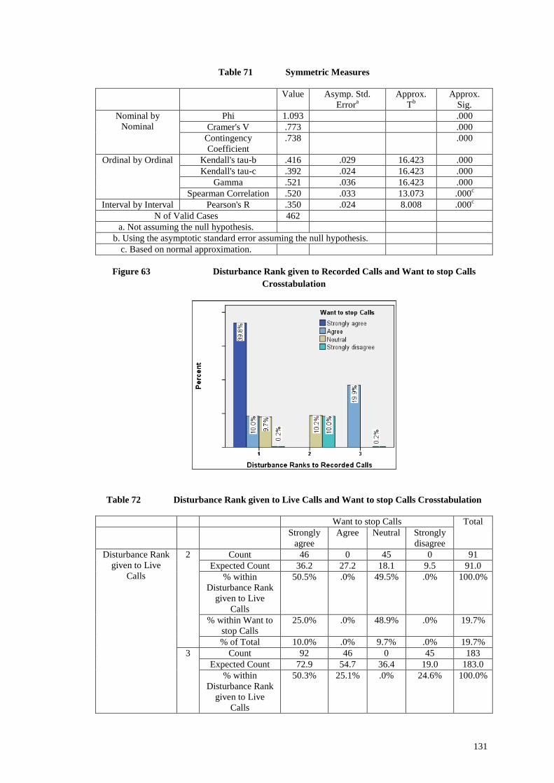
Table 71 Symmetric Measures
Value Asymp. Std.Errora
Approx.Tb
Approx.Sig.
Nominal byNominal
Phi 1.093 .000Cramer's V .773 .000
ContingencyCoefficient
.738 .000
Ordinal by Ordinal Kendall's tau-b .416 .029 16.423 .000Kendall's tau-c .392 .024 16.423 .000
Gamma .521 .036 16.423 .000Spearman Correlation .520 .033 13.073 .000c
Interval by Interval Pearson's R .350 .024 8.008 .000c
N of Valid Cases 462a. Not assuming the null hypothesis.
b. Using the asymptotic standard error assuming the null hypothesis.c. Based on normal approximation.
Figure 63 Disturbance Rank given to Recorded Calls and Want to stop Calls
Crosstabulation
Table 72 Disturbance Rank given to Live Calls and Want to stop Calls Crosstabulation
Want to stop Calls TotalStrongly
agreeAgree Neutral Strongly
disagreeDisturbance Rank
given to LiveCalls
2 Count 46 0 45 0 91Expected Count 36.2 27.2 18.1 9.5 91.0
% withinDisturbance Rank
given to LiveCalls
50.5% .0% 49.5% .0% 100.0%
% within Want tostop Calls
25.0% .0% 48.9% .0% 19.7%
% of Total 10.0% .0% 9.7% .0% 19.7%3 Count 92 46 0 45 183
Expected Count 72.9 54.7 36.4 19.0 183.0% within
Disturbance Rankgiven to Live
Calls
50.3% 25.1% .0% 24.6% 100.0%
132
% within Want tostop Calls
50.0% 33.3% .0% 93.8% 39.6%
% of Total 19.9% 10.0% .0% 9.7% 39.6%4 Count 0 0 47 3 50
Expected Count 19.9 14.9 10.0 5.2 50.0% within
Disturbance Rankgiven to Live
Calls
.0% .0% 94.0% 6.0% 100.0%
% within Want tostop Calls
.0% .0% 51.1% 6.2% 10.8%
% of Total .0% .0% 10.2% .6% 10.8%5 Count 46 92 0 0 138
Expected Count 55.0 41.2 27.5 14.3 138.0% within
Disturbance Rankgiven to Live
Calls
33.3% 66.7% .0% .0% 100.0%
% within Want tostop Calls
25.0% 66.7% .0% .0% 29.9%
% of Total 10.0% 19.9% .0% .0% 29.9%Total Count 184 138 92 48 462
Expected Count 184.0 138.0 92.0 48.0 462.0% within
Disturbance Rankgiven to Live
Calls
39.8% 29.9% 19.9% 10.4% 100.0%
% within Want tostop Calls
100.0% 100.0% 100.0% 100.0% 100.0%
% of Total 39.8% 29.9% 19.9% 10.4% 100.0%
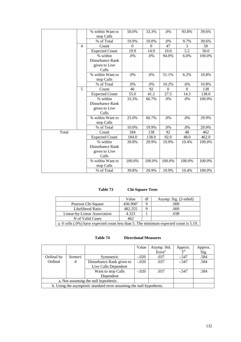
Table 73 Chi-Square Tests
Value df Asymp. Sig. (2-sided)Pearson Chi-Square 436.906a 9 .000
Likelihood Ratio 482.255 9 .000Linear-by-Linear Association 4.323 1 .038
N of Valid Cases 462a. 0 cells (.0%) have expected count less than 5. The minimum expected count is 5.19.
Table 74 Directional Measures
Value Asymp. Std.Errora
Approx.Tb
Approx.Sig.
Ordinal byOrdinal
Somers'd
Symmetric -.020 .037 -.547 .584Disturbance Rank given to
Live Calls Dependent-.020 .037 -.547 .584
Want to stop CallsDependent
-.020 .037 -.547 .584
a. Not assuming the null hypothesis.b. Using the asymptotic standard error assuming the null hypothesis.
133
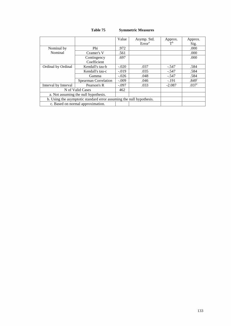
Table 75 Symmetric Measures
Value Asymp. Std.Errora
Approx.Tb
Approx.Sig.
Nominal byNominal
Phi .972 .000Cramer's V .561 .000
ContingencyCoefficient
.697 .000
Ordinal by Ordinal Kendall's tau-b -.020 .037 -.547 .584Kendall's tau-c -.019 .035 -.547 .584
Gamma -.026 .048 -.547 .584Spearman Correlation -.009 .046 -.191 .849c
Interval by Interval Pearson's R -.097 .033 -2.087 .037c
N of Valid Cases 462a. Not assuming the null hypothesis.
b. Using the asymptotic standard error assuming the null hypothesis.c. Based on normal approximation.
134
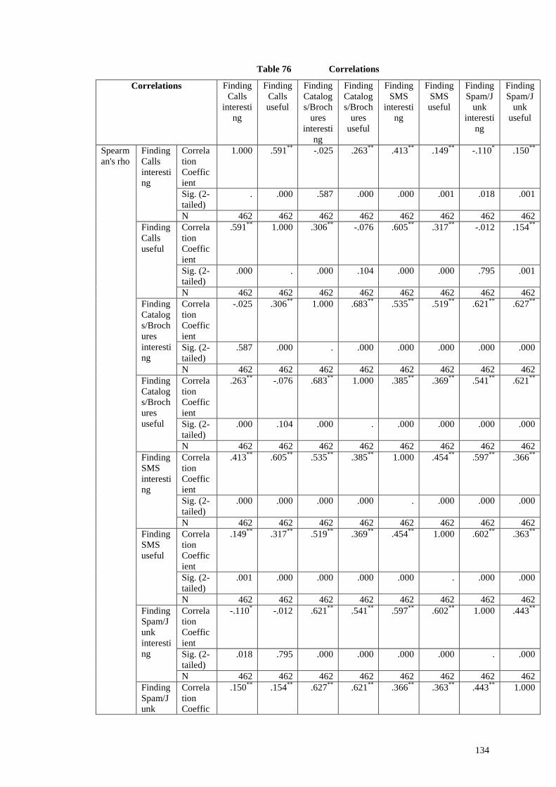
Table 76 Correlations
Correlations FindingCalls
interesting
FindingCallsuseful
FindingCatalogs/Broch
uresinteresti
ng
FindingCatalogs/Broch
uresuseful
FindingSMS
interesting
FindingSMSuseful
FindingSpam/J
unkinteresti
ng
FindingSpam/J
unkuseful
Spearman's rho
FindingCallsinteresting
CorrelationCoefficient
1.000 .591** -.025 .263** .413** .149** -.110* .150**
Sig. (2-tailed)
. .000 .587 .000 .000 .001 .018 .001
N 462 462 462 462 462 462 462 462FindingCallsuseful
CorrelationCoefficient
.591** 1.000 .306** -.076 .605** .317** -.012 .154**
Sig. (2-tailed)
.000 . .000 .104 .000 .000 .795 .001
N 462 462 462 462 462 462 462 462FindingCatalogs/Brochuresinteresting
CorrelationCoefficient
-.025 .306** 1.000 .683** .535** .519** .621** .627**
Sig. (2-tailed)
.587 .000 . .000 .000 .000 .000 .000
N 462 462 462 462 462 462 462 462FindingCatalogs/Brochuresuseful
CorrelationCoefficient
.263** -.076 .683** 1.000 .385** .369** .541** .621**
Sig. (2-tailed)
.000 .104 .000 . .000 .000 .000 .000
N 462 462 462 462 462 462 462 462FindingSMSinteresting
CorrelationCoefficient
.413** .605** .535** .385** 1.000 .454** .597** .366**
Sig. (2-tailed)
.000 .000 .000 .000 . .000 .000 .000
N 462 462 462 462 462 462 462 462FindingSMSuseful
CorrelationCoefficient
.149** .317** .519** .369** .454** 1.000 .602** .363**
Sig. (2-tailed)
.001 .000 .000 .000 .000 . .000 .000
N 462 462 462 462 462 462 462 462FindingSpam/Junkinteresting
CorrelationCoefficient
-.110* -.012 .621** .541** .597** .602** 1.000 .443**
Sig. (2-tailed)
.018 .795 .000 .000 .000 .000 . .000
N 462 462 462 462 462 462 462 462FindingSpam/Junk
CorrelationCoeffic
.150** .154** .627** .621** .366** .363** .443** 1.000
135
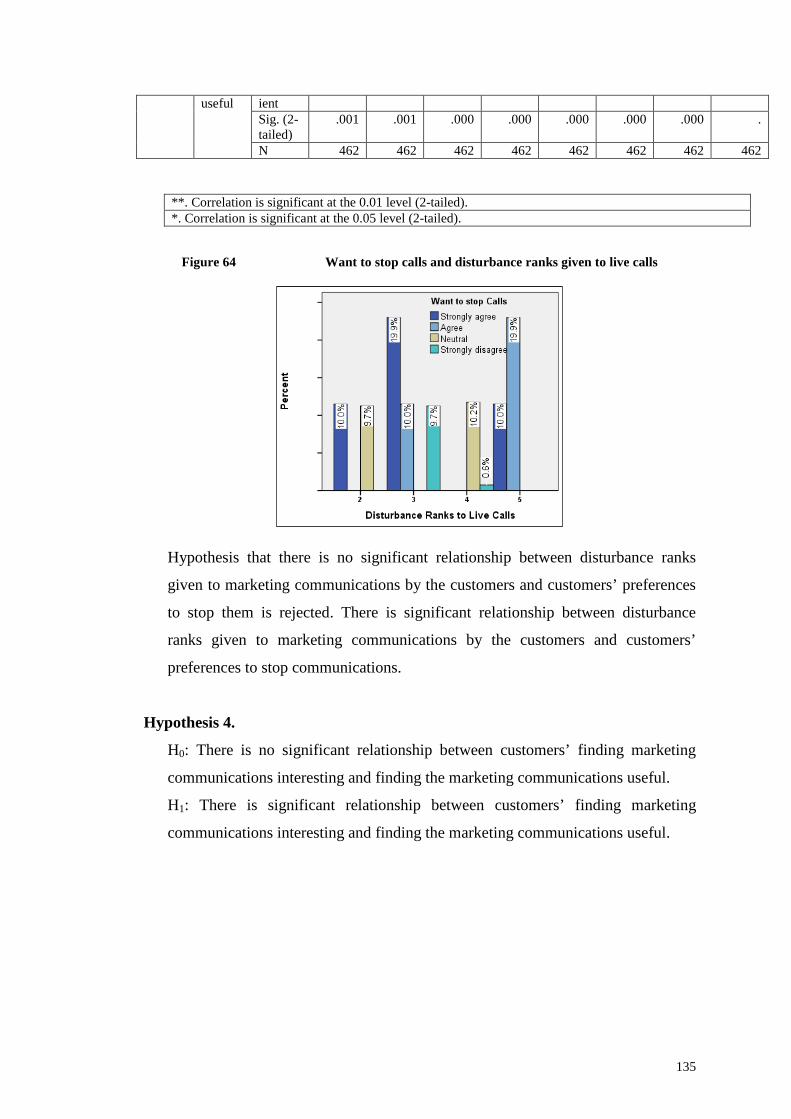
Figure 64 Want to stop calls and disturbance ranks given to live calls
Hypothesis that there is no significant relationship between disturbance ranks
given to marketing communications by the customers and customers’ preferences
to stop them is rejected. There is significant relationship between disturbance
ranks given to marketing communications by the customers and customers’
preferences to stop communications.
Hypothesis 4.
H0: There is no significant relationship between customers’ finding marketing
communications interesting and finding the marketing communications useful.
H1: There is significant relationship between customers’ finding marketing
communications interesting and finding the marketing communications useful.
useful ientSig. (2-tailed)
.001 .001 .000 .000 .000 .000 .000 .
N 462 462 462 462 462 462 462 462
**. Correlation is significant at the 0.01 level (2-tailed).*. Correlation is significant at the 0.05 level (2-tailed).
136
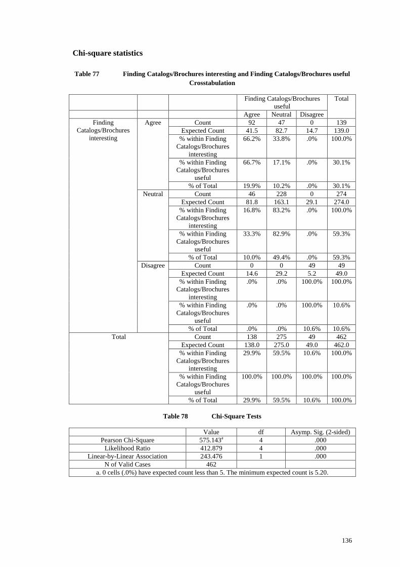
Chi-square statistics
Table 77 Finding Catalogs/Brochures interesting and Finding Catalogs/Brochures useful
Crosstabulation
Finding Catalogs/Brochuresuseful
Total
Agree Neutral DisagreeFinding
Catalogs/Brochuresinteresting
Agree Count 92 47 0 139Expected Count 41.5 82.7 14.7 139.0
% within FindingCatalogs/Brochures
interesting
66.2% 33.8% .0% 100.0%
% within FindingCatalogs/Brochures
useful
66.7% 17.1% .0% 30.1%
% of Total 19.9% 10.2% .0% 30.1%Neutral Count 46 228 0 274
Expected Count 81.8 163.1 29.1 274.0% within Finding
Catalogs/Brochuresinteresting
16.8% 83.2% .0% 100.0%
% within FindingCatalogs/Brochures
useful
33.3% 82.9% .0% 59.3%
% of Total 10.0% 49.4% .0% 59.3%Disagree Count 0 0 49 49
Expected Count 14.6 29.2 5.2 49.0% within Finding
Catalogs/Brochuresinteresting
.0% .0% 100.0% 100.0%
% within FindingCatalogs/Brochures
useful
.0% .0% 100.0% 10.6%
% of Total .0% .0% 10.6% 10.6%Total Count 138 275 49 462
Expected Count 138.0 275.0 49.0 462.0% within Finding
Catalogs/Brochuresinteresting
29.9% 59.5% 10.6% 100.0%
% within FindingCatalogs/Brochures
useful
100.0% 100.0% 100.0% 100.0%
% of Total 29.9% 59.5% 10.6% 100.0%
Table 78 Chi-Square Tests
Value df Asymp. Sig. (2-sided)Pearson Chi-Square 575.143a 4 .000
Likelihood Ratio 412.879 4 .000Linear-by-Linear Association 243.476 1 .000
N of Valid Cases 462a. 0 cells (.0%) have expected count less than 5. The minimum expected count is 5.20.
137
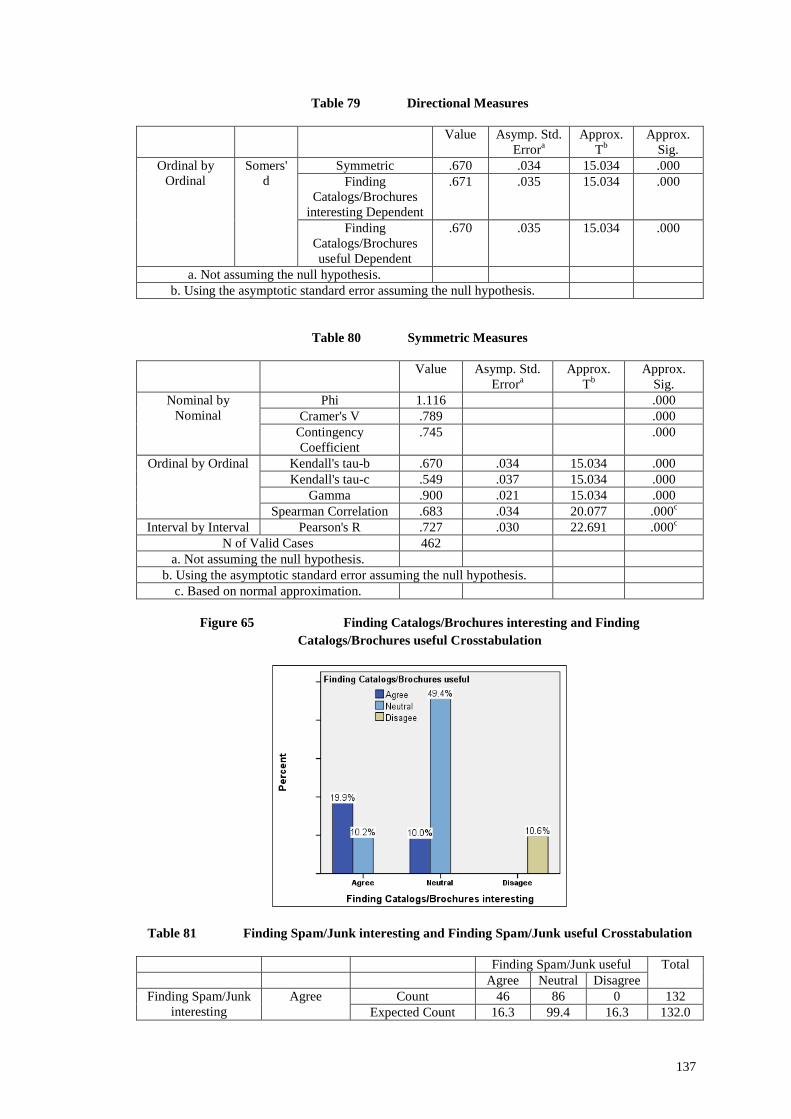
Table 79 Directional Measures
Value Asymp. Std.Errora
Approx.Tb
Approx.Sig.
Ordinal byOrdinal
Somers'd
Symmetric .670 .034 15.034 .000Finding
Catalogs/Brochuresinteresting Dependent
.671 .035 15.034 .000
FindingCatalogs/Brochuresuseful Dependent
.670 .035 15.034 .000
a. Not assuming the null hypothesis.b. Using the asymptotic standard error assuming the null hypothesis.
Table 80 Symmetric Measures
Value Asymp. Std.Errora
Approx.Tb
Approx.Sig.
Nominal byNominal
Phi 1.116 .000Cramer's V .789 .000
ContingencyCoefficient
.745 .000
Ordinal by Ordinal Kendall's tau-b .670 .034 15.034 .000Kendall's tau-c .549 .037 15.034 .000
Gamma .900 .021 15.034 .000Spearman Correlation .683 .034 20.077 .000c
Interval by Interval Pearson's R .727 .030 22.691 .000c
N of Valid Cases 462a. Not assuming the null hypothesis.
b. Using the asymptotic standard error assuming the null hypothesis.c. Based on normal approximation.
Figure 65 Finding Catalogs/Brochures interesting and Finding
Catalogs/Brochures useful Crosstabulation
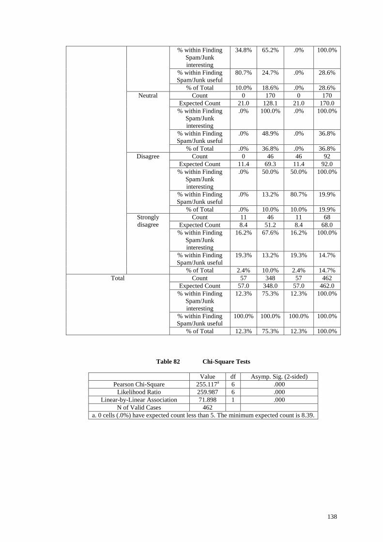
Table 81 Finding Spam/Junk interesting and Finding Spam/Junk useful Crosstabulation
Finding Spam/Junk useful TotalAgree Neutral Disagree
Finding Spam/Junkinteresting
Agree Count 46 86 0 132Expected Count 16.3 99.4 16.3 132.0
138
% within FindingSpam/Junkinteresting
34.8% 65.2% .0% 100.0%
% within FindingSpam/Junk useful
80.7% 24.7% .0% 28.6%
% of Total 10.0% 18.6% .0% 28.6%Neutral Count 0 170 0 170
Expected Count 21.0 128.1 21.0 170.0% within Finding
Spam/Junkinteresting
.0% 100.0% .0% 100.0%
% within FindingSpam/Junk useful
.0% 48.9% .0% 36.8%
% of Total .0% 36.8% .0% 36.8%Disagree Count 0 46 46 92
Expected Count 11.4 69.3 11.4 92.0% within Finding
Spam/Junkinteresting
.0% 50.0% 50.0% 100.0%
% within FindingSpam/Junk useful
.0% 13.2% 80.7% 19.9%
% of Total .0% 10.0% 10.0% 19.9%Stronglydisagree
Count 11 46 11 68Expected Count 8.4 51.2 8.4 68.0
% within FindingSpam/Junkinteresting
16.2% 67.6% 16.2% 100.0%
% within FindingSpam/Junk useful
19.3% 13.2% 19.3% 14.7%
% of Total 2.4% 10.0% 2.4% 14.7%Total Count 57 348 57 462
Expected Count 57.0 348.0 57.0 462.0% within Finding
Spam/Junkinteresting
12.3% 75.3% 12.3% 100.0%
% within FindingSpam/Junk useful
100.0% 100.0% 100.0% 100.0%
% of Total 12.3% 75.3% 12.3% 100.0%
Table 82 Chi-Square Tests
Value df Asymp. Sig. (2-sided)Pearson Chi-Square 255.117a 6 .000
Likelihood Ratio 259.987 6 .000Linear-by-Linear Association 71.898 1 .000
N of Valid Cases 462a. 0 cells (.0%) have expected count less than 5. The minimum expected count is 8.39.
139
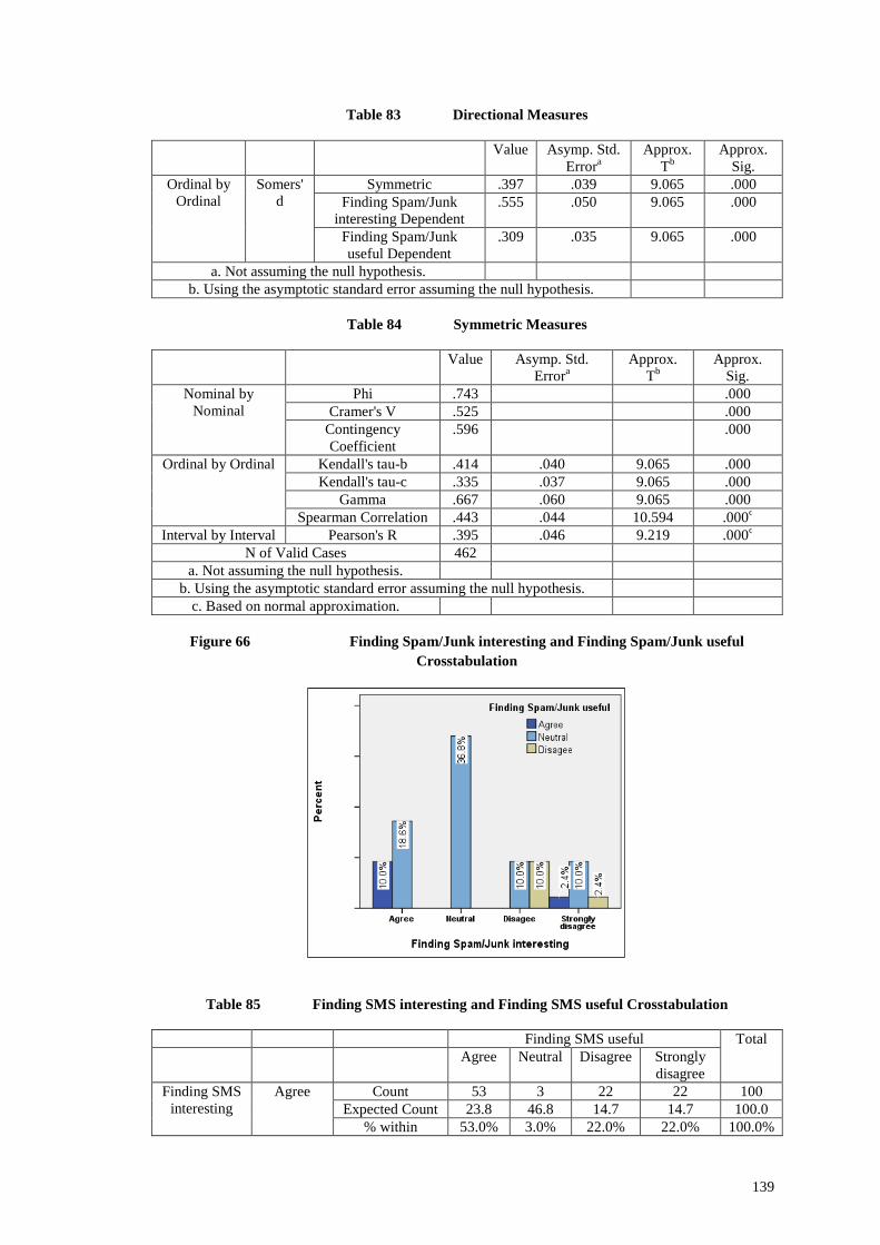
Table 83 Directional Measures
Value Asymp. Std.Errora
Approx.Tb
Approx.Sig.
Ordinal byOrdinal
Somers'd
Symmetric .397 .039 9.065 .000Finding Spam/Junk
interesting Dependent.555 .050 9.065 .000
Finding Spam/Junkuseful Dependent
.309 .035 9.065 .000
a. Not assuming the null hypothesis.b. Using the asymptotic standard error assuming the null hypothesis.
Table 84 Symmetric Measures
Value Asymp. Std.Errora
Approx.Tb
Approx.Sig.
Nominal byNominal
Phi .743 .000Cramer's V .525 .000
ContingencyCoefficient
.596 .000
Ordinal by Ordinal Kendall's tau-b .414 .040 9.065 .000Kendall's tau-c .335 .037 9.065 .000
Gamma .667 .060 9.065 .000Spearman Correlation .443 .044 10.594 .000c
Interval by Interval Pearson's R .395 .046 9.219 .000c
N of Valid Cases 462a. Not assuming the null hypothesis.
b. Using the asymptotic standard error assuming the null hypothesis.c. Based on normal approximation.
Figure 66 Finding Spam/Junk interesting and Finding Spam/Junk useful
Crosstabulation
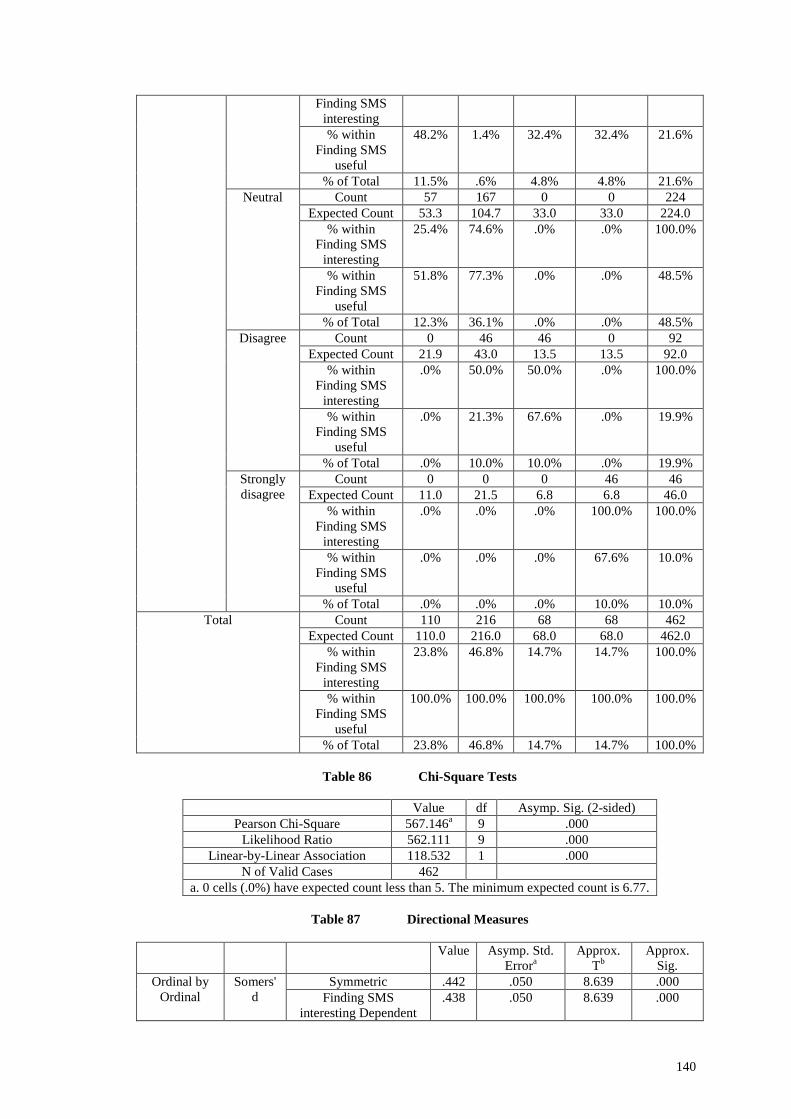
Table 85 Finding SMS interesting and Finding SMS useful Crosstabulation
Finding SMS useful TotalAgree Neutral Disagree Strongly
disagreeFinding SMS
interestingAgree Count 53 3 22 22 100
Expected Count 23.8 46.8 14.7 14.7 100.0% within 53.0% 3.0% 22.0% 22.0% 100.0%
140
Finding SMSinteresting% within
Finding SMSuseful
48.2% 1.4% 32.4% 32.4% 21.6%
% of Total 11.5% .6% 4.8% 4.8% 21.6%Neutral Count 57 167 0 0 224
Expected Count 53.3 104.7 33.0 33.0 224.0% within
Finding SMSinteresting
25.4% 74.6% .0% .0% 100.0%
% withinFinding SMS
useful
51.8% 77.3% .0% .0% 48.5%
% of Total 12.3% 36.1% .0% .0% 48.5%Disagree Count 0 46 46 0 92
Expected Count 21.9 43.0 13.5 13.5 92.0% within
Finding SMSinteresting
.0% 50.0% 50.0% .0% 100.0%
% withinFinding SMS
useful
.0% 21.3% 67.6% .0% 19.9%
% of Total .0% 10.0% 10.0% .0% 19.9%Stronglydisagree
Count 0 0 0 46 46Expected Count 11.0 21.5 6.8 6.8 46.0
% withinFinding SMS
interesting
.0% .0% .0% 100.0% 100.0%
% withinFinding SMS
useful
.0% .0% .0% 67.6% 10.0%
% of Total .0% .0% .0% 10.0% 10.0%Total Count 110 216 68 68 462
Expected Count 110.0 216.0 68.0 68.0 462.0% within
Finding SMSinteresting
23.8% 46.8% 14.7% 14.7% 100.0%
% withinFinding SMS
useful
100.0% 100.0% 100.0% 100.0% 100.0%
% of Total 23.8% 46.8% 14.7% 14.7% 100.0%
Table 86 Chi-Square Tests
Value df Asymp. Sig. (2-sided)Pearson Chi-Square 567.146a 9 .000
Likelihood Ratio 562.111 9 .000Linear-by-Linear Association 118.532 1 .000
N of Valid Cases 462a. 0 cells (.0%) have expected count less than 5. The minimum expected count is 6.77.
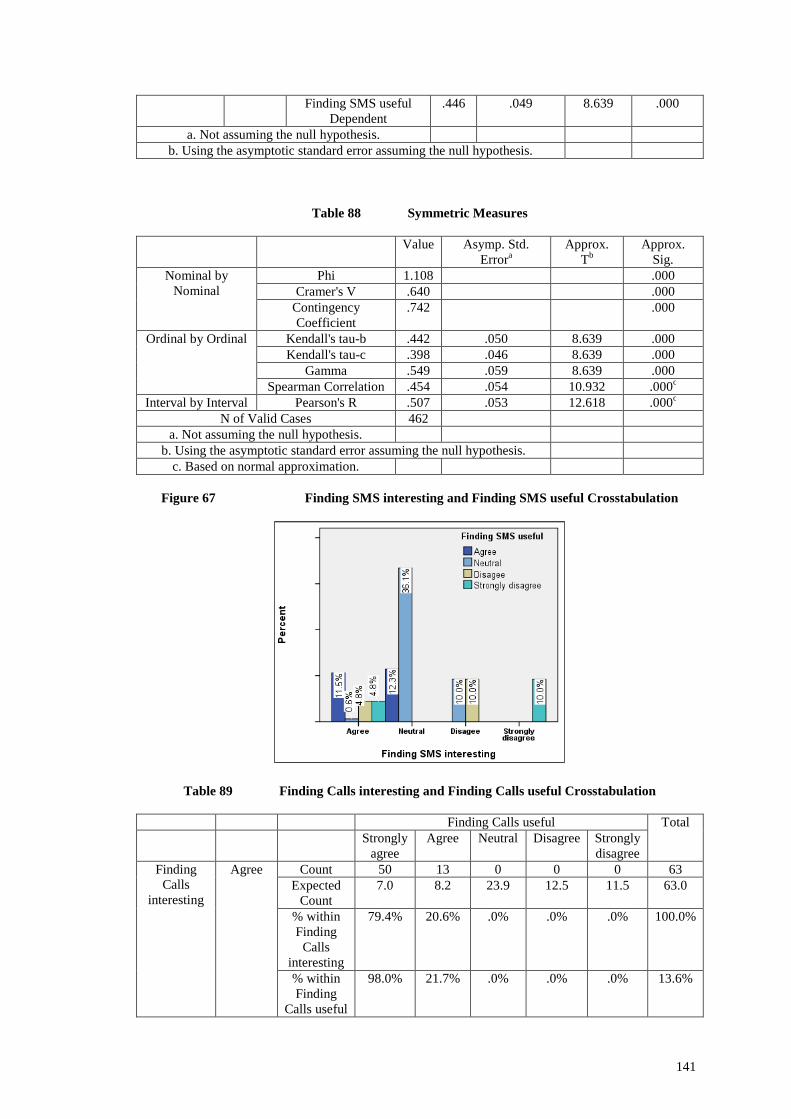
Table 87 Directional Measures
Value Asymp. Std.Errora
Approx.Tb
Approx.Sig.
Ordinal byOrdinal
Somers'd
Symmetric .442 .050 8.639 .000Finding SMS
interesting Dependent.438 .050 8.639 .000
141
Finding SMS usefulDependent
.446 .049 8.639 .000
a. Not assuming the null hypothesis.b. Using the asymptotic standard error assuming the null hypothesis.
Table 88 Symmetric Measures
Value Asymp. Std.Errora
Approx.Tb
Approx.Sig.
Nominal byNominal
Phi 1.108 .000Cramer's V .640 .000
ContingencyCoefficient
.742 .000
Ordinal by Ordinal Kendall's tau-b .442 .050 8.639 .000Kendall's tau-c .398 .046 8.639 .000
Gamma .549 .059 8.639 .000Spearman Correlation .454 .054 10.932 .000c
Interval by Interval Pearson's R .507 .053 12.618 .000c
N of Valid Cases 462a. Not assuming the null hypothesis.
b. Using the asymptotic standard error assuming the null hypothesis.c. Based on normal approximation.
Figure 67 Finding SMS interesting and Finding SMS useful Crosstabulation
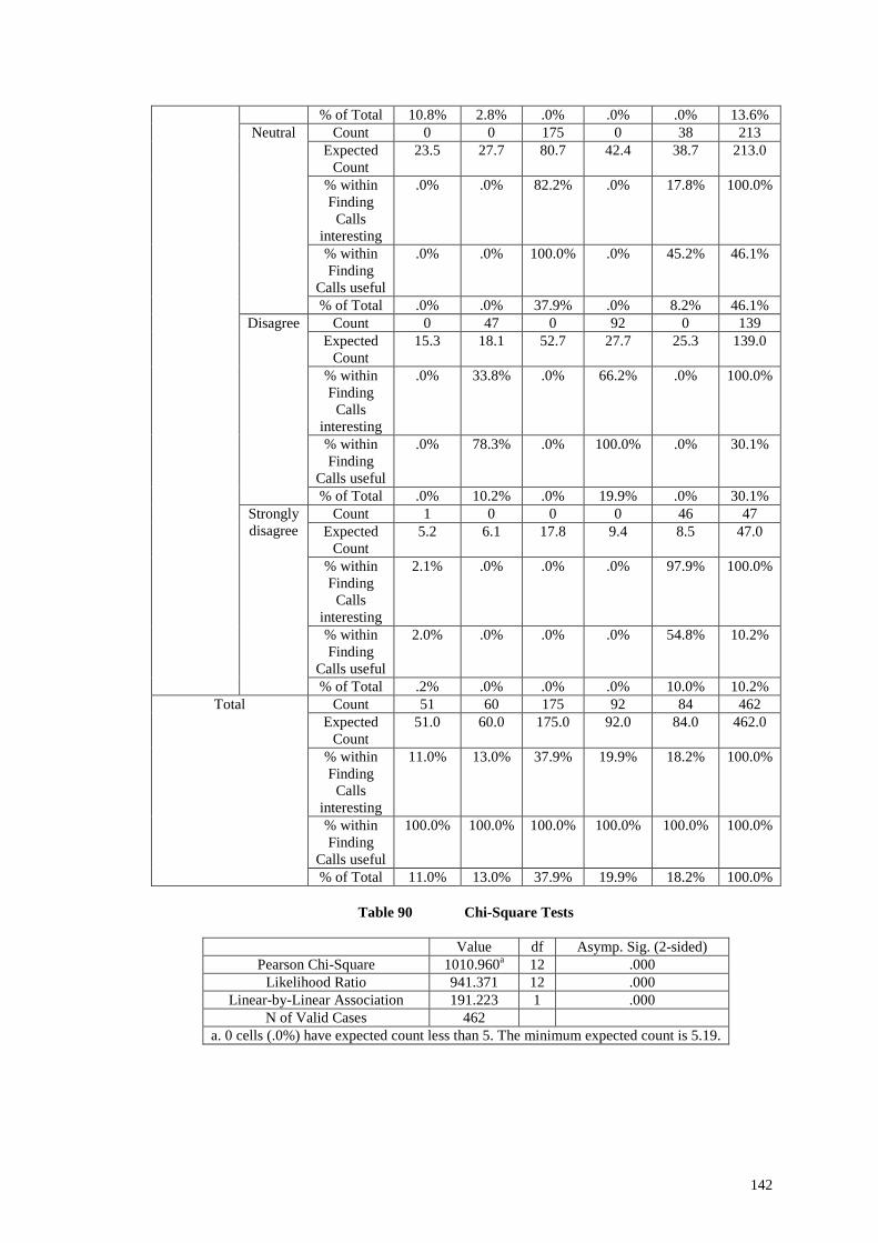
Table 89 Finding Calls interesting and Finding Calls useful Crosstabulation
Finding Calls useful TotalStrongly
agreeAgree Neutral Disagree Strongly
disagreeFinding
Callsinteresting
Agree Count 50 13 0 0 0 63Expected
Count7.0 8.2 23.9 12.5 11.5 63.0
% withinFinding
Callsinteresting
79.4% 20.6% .0% .0% .0% 100.0%
% withinFinding
Calls useful
98.0% 21.7% .0% .0% .0% 13.6%
142
% of Total 10.8% 2.8% .0% .0% .0% 13.6%Neutral Count 0 0 175 0 38 213
ExpectedCount
23.5 27.7 80.7 42.4 38.7 213.0
% withinFinding
Callsinteresting
.0% .0% 82.2% .0% 17.8% 100.0%
% withinFinding
Calls useful
.0% .0% 100.0% .0% 45.2% 46.1%
% of Total .0% .0% 37.9% .0% 8.2% 46.1%Disagree Count 0 47 0 92 0 139
ExpectedCount
15.3 18.1 52.7 27.7 25.3 139.0
% withinFinding
Callsinteresting
.0% 33.8% .0% 66.2% .0% 100.0%
% withinFinding
Calls useful
.0% 78.3% .0% 100.0% .0% 30.1%
% of Total .0% 10.2% .0% 19.9% .0% 30.1%Stronglydisagree
Count 1 0 0 0 46 47Expected
Count5.2 6.1 17.8 9.4 8.5 47.0
% withinFinding
Callsinteresting
2.1% .0% .0% .0% 97.9% 100.0%
% withinFinding
Calls useful
2.0% .0% .0% .0% 54.8% 10.2%
% of Total .2% .0% .0% .0% 10.0% 10.2%Total Count 51 60 175 92 84 462
ExpectedCount
51.0 60.0 175.0 92.0 84.0 462.0
% withinFinding
Callsinteresting
11.0% 13.0% 37.9% 19.9% 18.2% 100.0%
% withinFinding
Calls useful
100.0% 100.0% 100.0% 100.0% 100.0% 100.0%
% of Total 11.0% 13.0% 37.9% 19.9% 18.2% 100.0%
Table 90 Chi-Square Tests
Value df Asymp. Sig. (2-sided)Pearson Chi-Square 1010.960a 12 .000
Likelihood Ratio 941.371 12 .000Linear-by-Linear Association 191.223 1 .000
N of Valid Cases 462a. 0 cells (.0%) have expected count less than 5. The minimum expected count is 5.19.
143
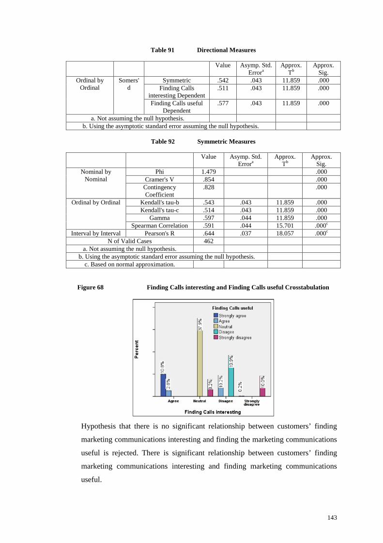
Table 91 Directional Measures
Value Asymp. Std.Errora
Approx.Tb
Approx.Sig.
Ordinal byOrdinal
Somers'd
Symmetric .542 .043 11.859 .000Finding Calls
interesting Dependent.511 .043 11.859 .000
Finding Calls usefulDependent
.577 .043 11.859 .000
a. Not assuming the null hypothesis.b. Using the asymptotic standard error assuming the null hypothesis.
Table 92 Symmetric Measures
Value Asymp. Std.Errora
Approx.Tb
Approx.Sig.
Nominal byNominal
Phi 1.479 .000Cramer's V .854 .000
ContingencyCoefficient
.828 .000
Ordinal by Ordinal Kendall's tau-b .543 .043 11.859 .000Kendall's tau-c .514 .043 11.859 .000
Gamma .597 .044 11.859 .000Spearman Correlation .591 .044 15.701 .000c
Interval by Interval Pearson's R .644 .037 18.057 .000c
N of Valid Cases 462a. Not assuming the null hypothesis.
b. Using the asymptotic standard error assuming the null hypothesis.c. Based on normal approximation.
Figure 68 Finding Calls interesting and Finding Calls useful Crosstabulation
Hypothesis that there is no significant relationship between customers’ finding
marketing communications interesting and finding the marketing communications
useful is rejected. There is significant relationship between customers’ finding
marketing communications interesting and finding marketing communications
useful.
144
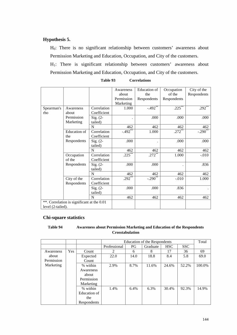
Hypothesis 5.
H0: There is no significant relationship between customers’ awareness about
Permission Marketing and Education, Occupation, and City of the customers.
H1: There is significant relationship between customers’ awareness about
Permission Marketing and Education, Occupation, and City of the customers.
Table 93 Correlations
Awarenessabout
PermissionMarketing
Education ofthe
Respondents
Occupationof the
Respondents
City of theRespondents
Spearman'srho
AwarenessaboutPermissionMarketing
CorrelationCoefficient
1.000 -.492** .225** .292**
Sig. (2-tailed)
. .000 .000 .000
N 462 462 462 462Education oftheRespondents
CorrelationCoefficient
-.492** 1.000 .272** -.290**
Sig. (2-tailed)
.000 . .000 .000
N 462 462 462 462Occupationof theRespondents
CorrelationCoefficient
.225** .272** 1.000 -.010
Sig. (2-tailed)
.000 .000 . .836
N 462 462 462 462City of theRespondents
CorrelationCoefficient
.292** -.290** -.010 1.000
Sig. (2-tailed)
.000 .000 .836 .
N 462 462 462 462**. Correlation is significant at the 0.01level (2-tailed).
Chi-square statistics
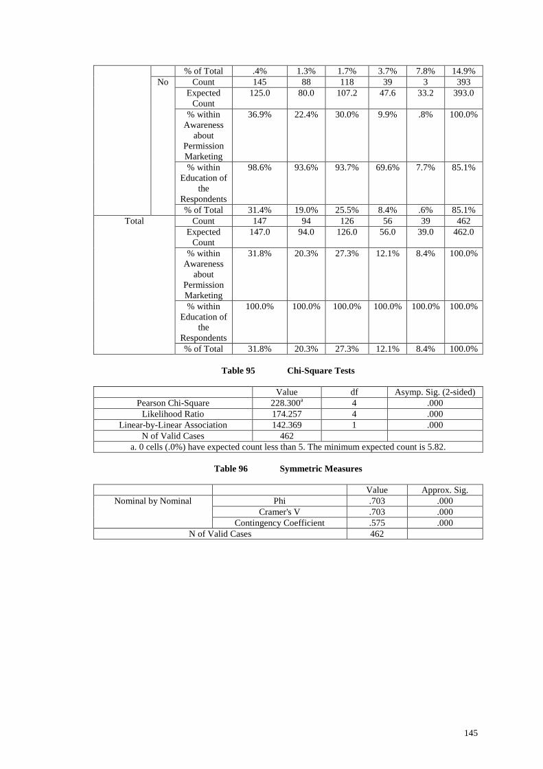
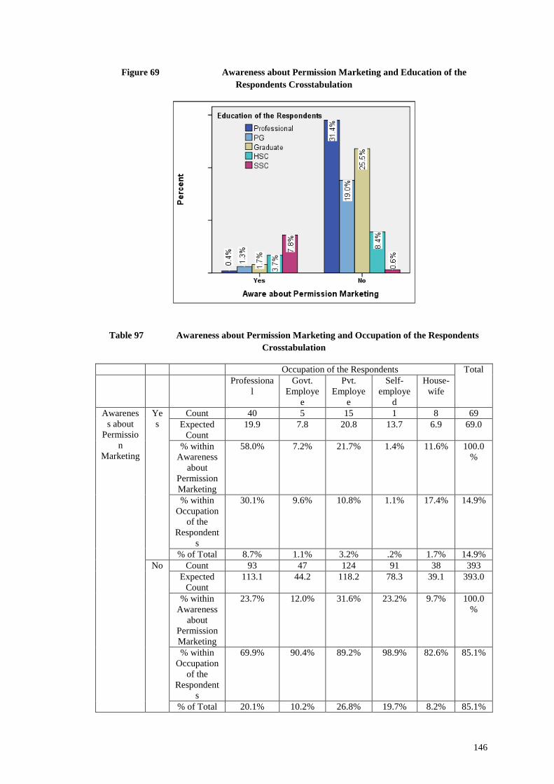
Table 94 Awareness about Permission Marketing and Education of the Respondents
Crosstabulation
Education of the Respondents TotalProfessional PG Graduate HSC SSC
Awarenessabout
PermissionMarketing
Yes Count 2 6 8 17 36 69Expected
Count22.0 14.0 18.8 8.4 5.8 69.0
% withinAwareness
aboutPermissionMarketing
2.9% 8.7% 11.6% 24.6% 52.2% 100.0%
% withinEducation of
theRespondents
1.4% 6.4% 6.3% 30.4% 92.3% 14.9%
145
% of Total .4% 1.3% 1.7% 3.7% 7.8% 14.9%No Count 145 88 118 39 3 393
ExpectedCount
125.0 80.0 107.2 47.6 33.2 393.0
% withinAwareness
aboutPermissionMarketing
36.9% 22.4% 30.0% 9.9% .8% 100.0%
% withinEducation of
theRespondents
98.6% 93.6% 93.7% 69.6% 7.7% 85.1%
% of Total 31.4% 19.0% 25.5% 8.4% .6% 85.1%Total Count 147 94 126 56 39 462
ExpectedCount
147.0 94.0 126.0 56.0 39.0 462.0
% withinAwareness
aboutPermissionMarketing
31.8% 20.3% 27.3% 12.1% 8.4% 100.0%
% withinEducation of
theRespondents
100.0% 100.0% 100.0% 100.0% 100.0% 100.0%
% of Total 31.8% 20.3% 27.3% 12.1% 8.4% 100.0%
Table 95 Chi-Square Tests
Value df Asymp. Sig. (2-sided)Pearson Chi-Square 228.300a 4 .000
Likelihood Ratio 174.257 4 .000Linear-by-Linear Association 142.369 1 .000
N of Valid Cases 462a. 0 cells (.0%) have expected count less than 5. The minimum expected count is 5.82.
Table 96 Symmetric Measures
Value Approx. Sig.Nominal by Nominal Phi .703 .000
Cramer's V .703 .000Contingency Coefficient .575 .000
N of Valid Cases 462
146
Figure 69 Awareness about Permission Marketing and Education of the
Respondents Crosstabulation
Table 97 Awareness about Permission Marketing and Occupation of the Respondents
Crosstabulation
Occupation of the Respondents TotalProfessiona
lGovt.
Employee
Pvt.Employe
e
Self-employe
d
House-wife
Awareness about
Permission
Marketing
Yes
Count 40 5 15 1 8 69Expected
Count19.9 7.8 20.8 13.7 6.9 69.0
% withinAwareness
aboutPermissionMarketing
58.0% 7.2% 21.7% 1.4% 11.6% 100.0%
% withinOccupation
of theRespondent
s
30.1% 9.6% 10.8% 1.1% 17.4% 14.9%
% of Total 8.7% 1.1% 3.2% .2% 1.7% 14.9%No Count 93 47 124 91 38 393
ExpectedCount
113.1 44.2 118.2 78.3 39.1 393.0
% withinAwareness
aboutPermissionMarketing
23.7% 12.0% 31.6% 23.2% 9.7% 100.0%
% withinOccupation
of theRespondent
s
69.9% 90.4% 89.2% 98.9% 82.6% 85.1%
% of Total 20.1% 10.2% 26.8% 19.7% 8.2% 85.1%
147
Total Count 133 52 139 92 46 462Expected
Count133.0 52.0 139.0 92.0 46.0 462.0
% withinAwareness
aboutPermissionMarketing
28.8% 11.3% 30.1% 19.9% 10.0% 100.0%
% withinOccupation
of theRespondent
s
100.0% 100.0% 100.0% 100.0% 100.0%
100.0%
% of Total 28.8% 11.3% 30.1% 19.9% 10.0% 100.0%
Table 98 Chi-Square Tests
Value df Asymp. Sig. (2-sided)Pearson Chi-Square 41.139a 4 .000
Likelihood Ratio 45.308 4 .000Linear-by-Linear Association 16.068 1 .000
N of Valid Cases 462a. 0 cells (.0%) have expected count less than 5. The minimum expected count is 6.87.
Table 99 Symmetric Measures
Value Approx. Sig.Nominal by Nominal Phi .298 .000
Cramer's V .298 .000Contingency Coefficient .286 .000
N of Valid Cases 462
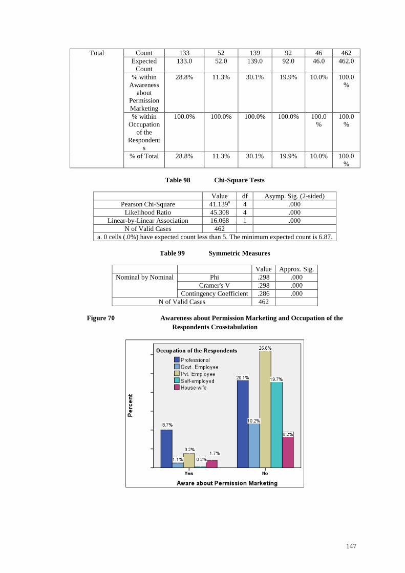
Figure 70 Awareness about Permission Marketing and Occupation of the
Respondents Crosstabulation
148
Table 100 Awareness about Permission Marketing and City of the Respondents
Crosstabulation
City of the Respondents TotalAhmedabad Baroda Surat Rajkot Jamnagar Anand
Awarenessabout
PermissionMarketing
Yes Count 30 21 4 4 3 7 69Expected
Count11.9 11.8 11.6 11.2 11.2 11.2 69.0
% withinAwareness
aboutPermissionMarketing
43.5% 30.4% 5.8% 5.8% 4.3% 10.1% 100.0%
% withinCity of the
Respondents
37.5% 26.6% 5.1% 5.3% 4.0% 9.3% 14.9%
% of Total 6.5% 4.5% .9% .9% .6% 1.5% 14.9%No Count 50 58 74 71 72 68 393
ExpectedCount
68.1 67.2 66.4 63.8 63.8 63.8 393.0
% withinAwareness
aboutPermissionMarketing
12.7% 14.8% 18.8% 18.1% 18.3% 17.3% 100.0%
% withinCity of the
Respondents
62.5% 73.4% 94.9% 94.7% 96.0% 90.7% 85.1%
% of Total 10.8% 12.6% 16.0% 15.4% 15.6% 14.7% 85.1%Total Count 80 79 78 75 75 75 462
ExpectedCount
80.0 79.0 78.0 75.0 75.0 75.0 462.0
% withinAwareness
aboutPermissionMarketing
17.3% 17.1% 16.9% 16.2% 16.2% 16.2% 100.0%
% withinCity of the
Respondents
100.0% 100.0% 100.0% 100.0% 100.0% 100.0% 100.0%
% of Total 17.3% 17.1% 16.9% 16.2% 16.2% 16.2% 100.0%
Table 101 Chi-Square Tests
Value Df Asymp. Sig. (2-sided)Pearson Chi-Square 60.757a 5 .000
Likelihood Ratio 57.693 5 .000Linear-by-Linear Association 38.581 1 .000
N of Valid Cases 462a. 0 cells (.0%) have expected count less than 5. The minimum expected count is 11.20.
Table 102 Symmetric Measures
Value Approx. Sig.Nominal by Nominal Phi .363 .000
Cramer's V .363 .000Contingency Coefficient .341 .000
N of Valid Cases 462
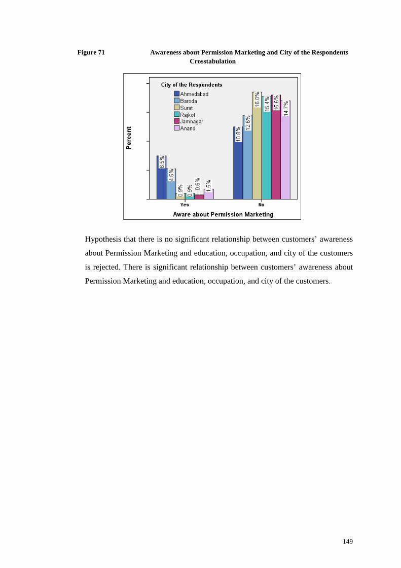
149
Figure 71 Awareness about Permission Marketing and City of the Respondents
Crosstabulation
Hypothesis that there is no significant relationship between customers’ awareness
about Permission Marketing and education, occupation, and city of the customers
is rejected. There is significant relationship between customers’ awareness about
Permission Marketing and education, occupation, and city of the customers.
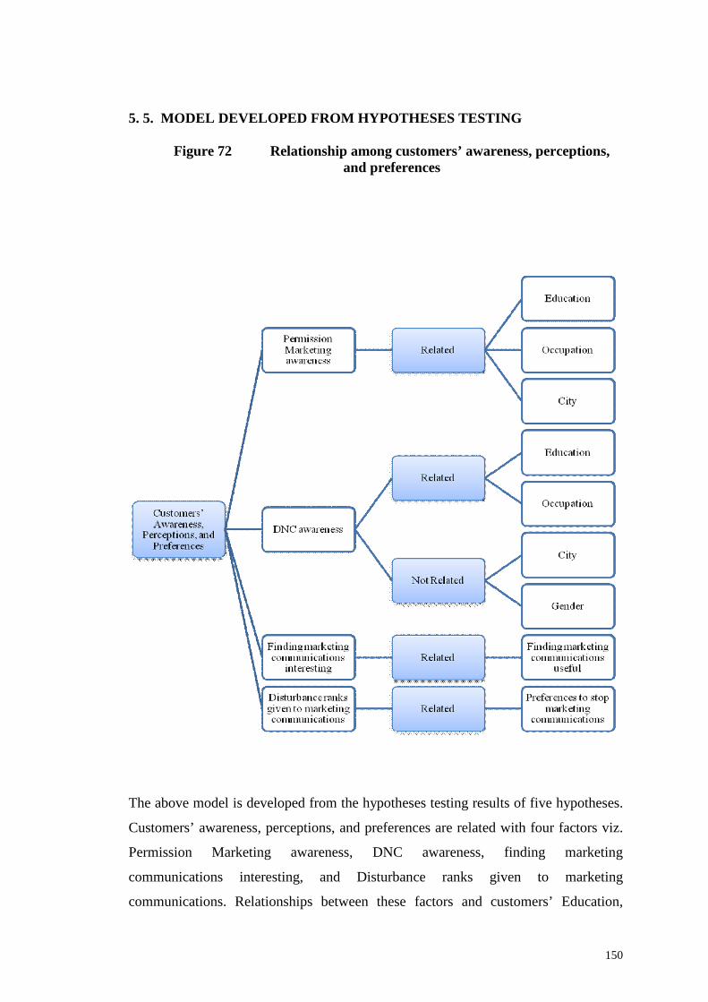
150
5. 5. MODEL DEVELOPED FROM HYPOTHESES TESTING
Figure 72 Relationship among customers’ awareness, perceptions,and preferences
The above model is developed from the hypotheses testing results of five hypotheses.
Customers’ awareness, perceptions, and preferences are related with four factors viz.
Permission Marketing awareness, DNC awareness, finding marketing
communications interesting, and Disturbance ranks given to marketing
communications. Relationships between these factors and customers’ Education,
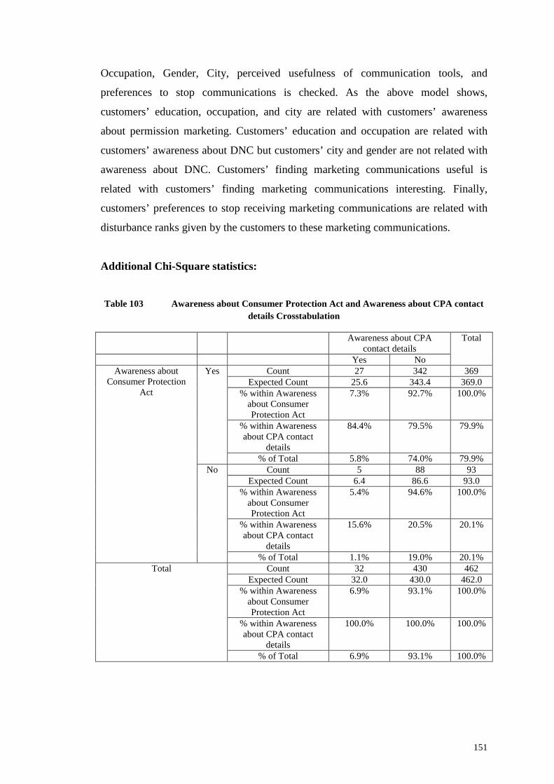
151
Occupation, Gender, City, perceived usefulness of communication tools, and
preferences to stop communications is checked. As the above model shows,
customers’ education, occupation, and city are related with customers’ awareness
about permission marketing. Customers’ education and occupation are related with
customers’ awareness about DNC but customers’ city and gender are not related with
awareness about DNC. Customers’ finding marketing communications useful is
related with customers’ finding marketing communications interesting. Finally,
customers’ preferences to stop receiving marketing communications are related with
disturbance ranks given by the customers to these marketing communications.
Additional Chi-Square statistics:
Table 103 Awareness about Consumer Protection Act and Awareness about CPA contact
details Crosstabulation
Awareness about CPAcontact details
Total
Yes NoAwareness about
Consumer ProtectionAct
Yes Count 27 342 369Expected Count 25.6 343.4 369.0
% within Awarenessabout ConsumerProtection Act
7.3% 92.7% 100.0%
% within Awarenessabout CPA contact
details
84.4% 79.5% 79.9%
% of Total 5.8% 74.0% 79.9%No Count 5 88 93
Expected Count 6.4 86.6 93.0% within Awareness
about ConsumerProtection Act
5.4% 94.6% 100.0%
% within Awarenessabout CPA contact
details
15.6% 20.5% 20.1%
% of Total 1.1% 19.0% 20.1%Total Count 32 430 462
Expected Count 32.0 430.0 462.0% within Awareness
about ConsumerProtection Act
6.9% 93.1% 100.0%
% within Awarenessabout CPA contact
details
100.0% 100.0% 100.0%
% of Total 6.9% 93.1% 100.0%
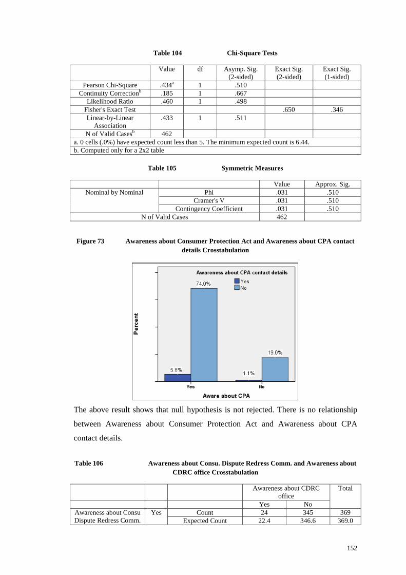
152
Table 104 Chi-Square Tests
Value df Asymp. Sig.(2-sided)
Exact Sig.(2-sided)
Exact Sig.(1-sided)
Pearson Chi-Square .434a 1 .510Continuity Correctionb .185 1 .667
Likelihood Ratio .460 1 .498Fisher's Exact Test .650 .346Linear-by-Linear
Association.433 1 .511
N of Valid Casesb 462a. 0 cells (.0%) have expected count less than 5. The minimum expected count is 6.44.b. Computed only for a 2x2 table
Table 105 Symmetric Measures
Value Approx. Sig.Nominal by Nominal Phi .031 .510
Cramer's V .031 .510Contingency Coefficient .031 .510
N of Valid Cases 462
Figure 73 Awareness about Consumer Protection Act and Awareness about CPA contact
details Crosstabulation
The above result shows that null hypothesis is not rejected. There is no relationship
between Awareness about Consumer Protection Act and Awareness about CPA
contact details.
Table 106 Awareness about Consu. Dispute Redress Comm. and Awareness about
CDRC office Crosstabulation
Awareness about CDRCoffice
Total
Yes NoAwareness about ConsuDispute Redress Comm.
Yes Count 24 345 369Expected Count 22.4 346.6 369.0
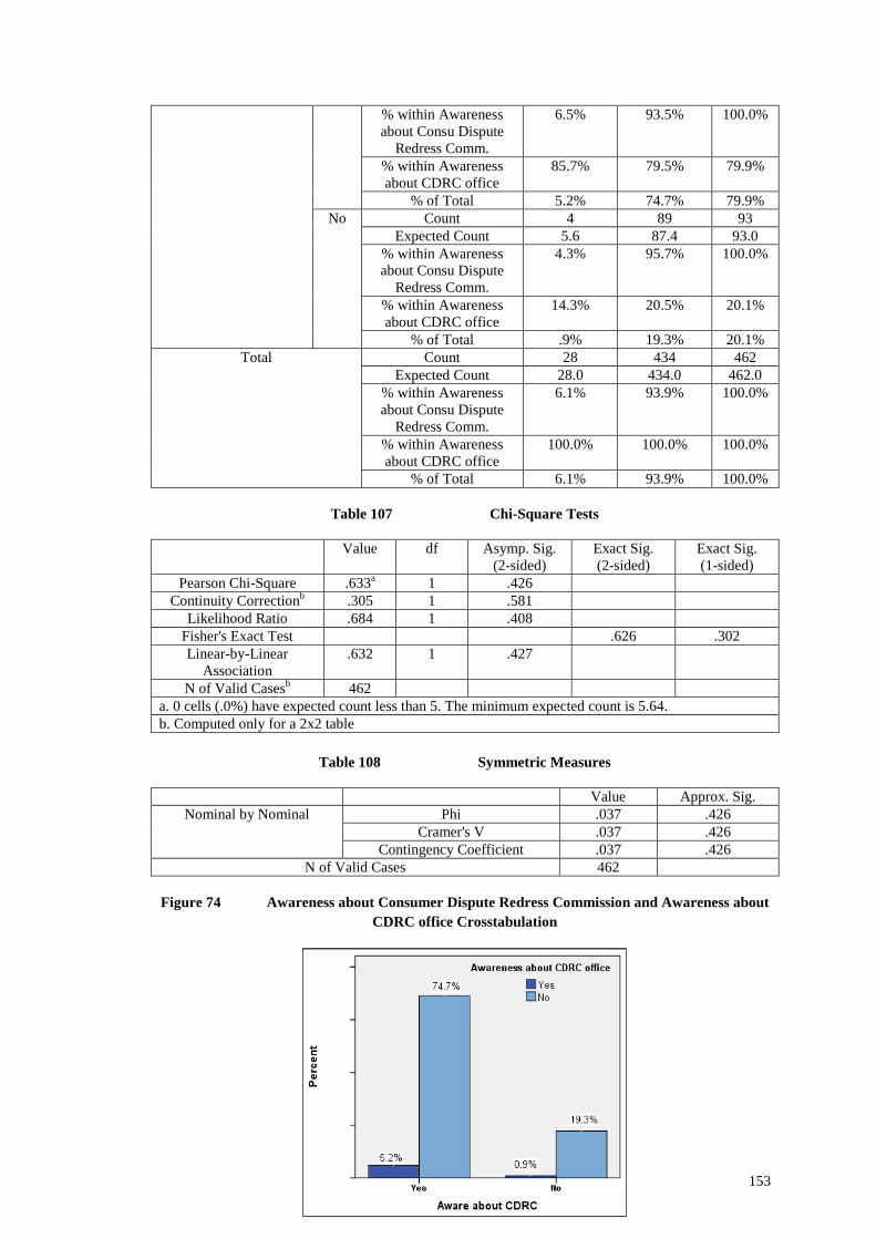
153
% within Awarenessabout Consu Dispute
Redress Comm.
6.5% 93.5% 100.0%
% within Awarenessabout CDRC office
85.7% 79.5% 79.9%
% of Total 5.2% 74.7% 79.9%No Count 4 89 93
Expected Count 5.6 87.4 93.0% within Awarenessabout Consu Dispute
Redress Comm.
4.3% 95.7% 100.0%
% within Awarenessabout CDRC office
14.3% 20.5% 20.1%
% of Total .9% 19.3% 20.1%Total Count 28 434 462
Expected Count 28.0 434.0 462.0% within Awarenessabout Consu Dispute
Redress Comm.
6.1% 93.9% 100.0%
% within Awarenessabout CDRC office
100.0% 100.0% 100.0%
% of Total 6.1% 93.9% 100.0%
Table 107 Chi-Square Tests
Value df Asymp. Sig.(2-sided)
Exact Sig.(2-sided)
Exact Sig.(1-sided)
Pearson Chi-Square .633a 1 .426Continuity Correctionb .305 1 .581
Likelihood Ratio .684 1 .408Fisher's Exact Test .626 .302Linear-by-Linear
Association.632 1 .427
N of Valid Casesb 462a. 0 cells (.0%) have expected count less than 5. The minimum expected count is 5.64.b. Computed only for a 2x2 table
Table 108 Symmetric Measures
Value Approx. Sig.Nominal by Nominal Phi .037 .426
Cramer's V .037 .426Contingency Coefficient .037 .426
N of Valid Cases 462
Figure 74 Awareness about Consumer Dispute Redress Commission and Awareness about
CDRC office Crosstabulation
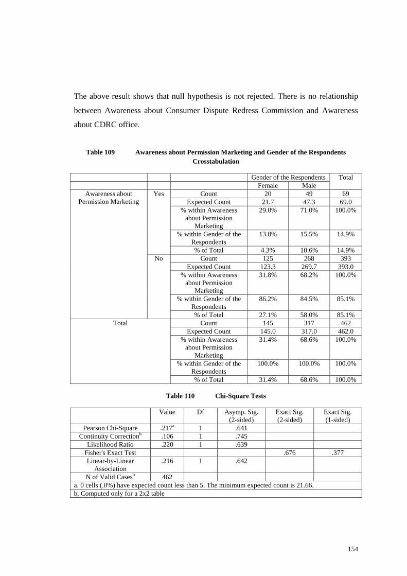
154
The above result shows that null hypothesis is not rejected. There is no relationship
between Awareness about Consumer Dispute Redress Commission and Awareness
about CDRC office.
Table 109 Awareness about Permission Marketing and Gender of the Respondents
Crosstabulation
Gender of the Respondents TotalFemale Male
Awareness aboutPermission Marketing
Yes Count 20 49 69Expected Count 21.7 47.3 69.0
% within Awarenessabout Permission
Marketing
29.0% 71.0% 100.0%
% within Gender of theRespondents
13.8% 15.5% 14.9%
% of Total 4.3% 10.6% 14.9%No Count 125 268 393
Expected Count 123.3 269.7 393.0% within Awareness
about PermissionMarketing
31.8% 68.2% 100.0%
% within Gender of theRespondents
86.2% 84.5% 85.1%
% of Total 27.1% 58.0% 85.1%Total Count 145 317 462
Expected Count 145.0 317.0 462.0% within Awareness
about PermissionMarketing
31.4% 68.6% 100.0%
% within Gender of theRespondents
100.0% 100.0% 100.0%
% of Total 31.4% 68.6% 100.0%
Table 110 Chi-Square Tests
Value Df Asymp. Sig.(2-sided)
Exact Sig.(2-sided)
Exact Sig.(1-sided)
Pearson Chi-Square .217a 1 .641Continuity Correctionb .106 1 .745
Likelihood Ratio .220 1 .639Fisher's Exact Test .676 .377Linear-by-Linear
Association.216 1 .642
N of Valid Casesb 462a. 0 cells (.0%) have expected count less than 5. The minimum expected count is 21.66.b. Computed only for a 2x2 table
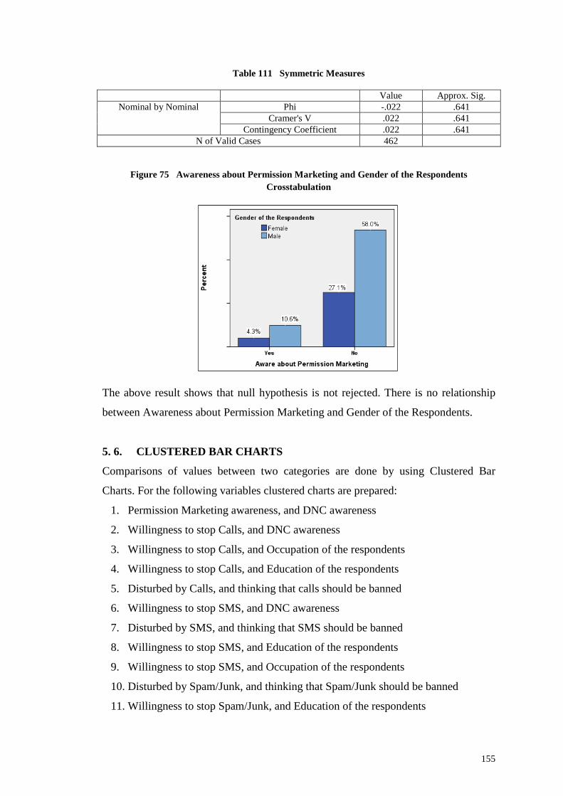
155
Table 111 Symmetric Measures
Value Approx. Sig.Nominal by Nominal Phi -.022 .641
Cramer's V .022 .641Contingency Coefficient .022 .641
N of Valid Cases 462
Figure 75 Awareness about Permission Marketing and Gender of the Respondents
Crosstabulation
The above result shows that null hypothesis is not rejected. There is no relationship
between Awareness about Permission Marketing and Gender of the Respondents.
5. 6. CLUSTERED BAR CHARTS
Comparisons of values between two categories are done by using Clustered Bar
Charts. For the following variables clustered charts are prepared:
1. Permission Marketing awareness, and DNC awareness
2. Willingness to stop Calls, and DNC awareness
3. Willingness to stop Calls, and Occupation of the respondents
4. Willingness to stop Calls, and Education of the respondents
5. Disturbed by Calls, and thinking that calls should be banned
6. Willingness to stop SMS, and DNC awareness
7. Disturbed by SMS, and thinking that SMS should be banned
8. Willingness to stop SMS, and Education of the respondents
9. Willingness to stop SMS, and Occupation of the respondents
10. Disturbed by Spam/Junk, and thinking that Spam/Junk should be banned
11. Willingness to stop Spam/Junk, and Education of the respondents
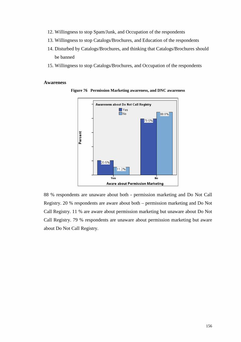
156
12. Willingness to stop Spam/Junk, and Occupation of the respondents
13. Willingness to stop Catalogs/Brochures, and Education of the respondents
14. Disturbed by Catalogs/Brochures, and thinking that Catalogs/Brochures should
be banned
15. Willingness to stop Catalogs/Brochures, and Occupation of the respondents
Awareness
Figure 76 Permission Marketing awareness, and DNC awareness
88 % respondents are unaware about both - permission marketing and Do Not Call
Registry. 20 % respondents are aware about both – permission marketing and Do Not
Call Registry. 11 % are aware about permission marketing but unaware about Do Not
Call Registry. 79 % respondents are unaware about permission marketing but aware
about Do Not Call Registry.
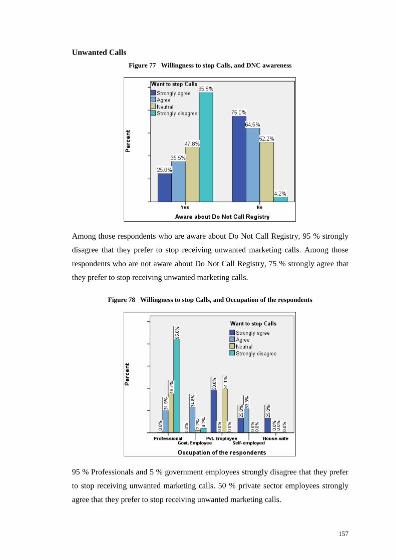
157
Unwanted Calls
Figure 77 Willingness to stop Calls, and DNC awareness
Among those respondents who are aware about Do Not Call Registry, 95 % strongly
disagree that they prefer to stop receiving unwanted marketing calls. Among those
respondents who are not aware about Do Not Call Registry, 75 % strongly agree that
they prefer to stop receiving unwanted marketing calls.
Figure 78 Willingness to stop Calls, and Occupation of the respondents
95 % Professionals and 5 % government employees strongly disagree that they prefer
to stop receiving unwanted marketing calls. 50 % private sector employees strongly
agree that they prefer to stop receiving unwanted marketing calls.
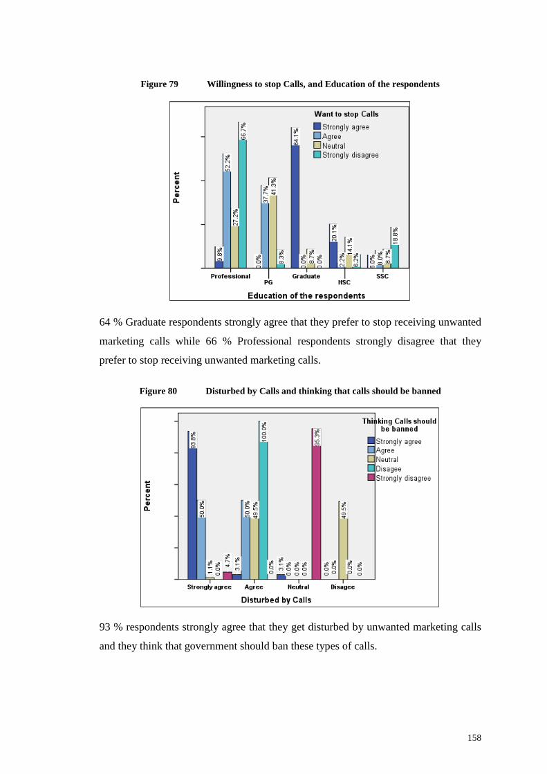
158
Figure 79 Willingness to stop Calls, and Education of the respondents
64 % Graduate respondents strongly agree that they prefer to stop receiving unwanted
marketing calls while 66 % Professional respondents strongly disagree that they
prefer to stop receiving unwanted marketing calls.
Figure 80 Disturbed by Calls and thinking that calls should be banned
93 % respondents strongly agree that they get disturbed by unwanted marketing calls
and they think that government should ban these types of calls.
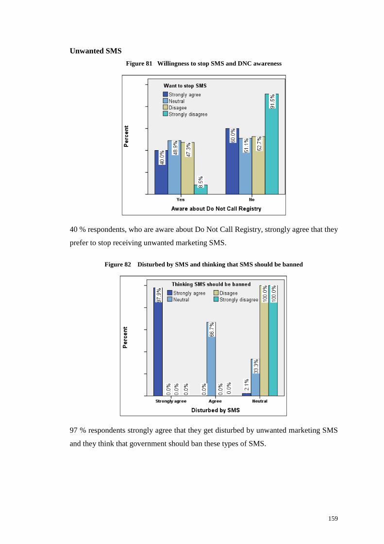
159
Unwanted SMS
Figure 81 Willingness to stop SMS and DNC awareness
40 % respondents, who are aware about Do Not Call Registry, strongly agree that they
prefer to stop receiving unwanted marketing SMS.
Figure 82 Disturbed by SMS and thinking that SMS should be banned
97 % respondents strongly agree that they get disturbed by unwanted marketing SMS
and they think that government should ban these types of SMS.
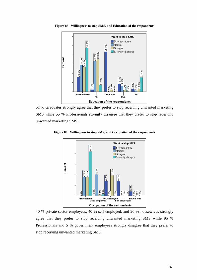
160
Figure 83 Willingness to stop SMS, and Education of the respondents
51 % Graduates strongly agree that they prefer to stop receiving unwanted marketing
SMS while 55 % Professionals strongly disagree that they prefer to stop receiving
unwanted marketing SMS.
Figure 84 Willingness to stop SMS, and Occupation of the respondents
40 % private sector employees, 40 % self-employed, and 20 % housewives strongly
agree that they prefer to stop receiving unwanted marketing SMS while 95 %
Professionals and 5 % government employees strongly disagree that they prefer to
stop receiving unwanted marketing SMS.
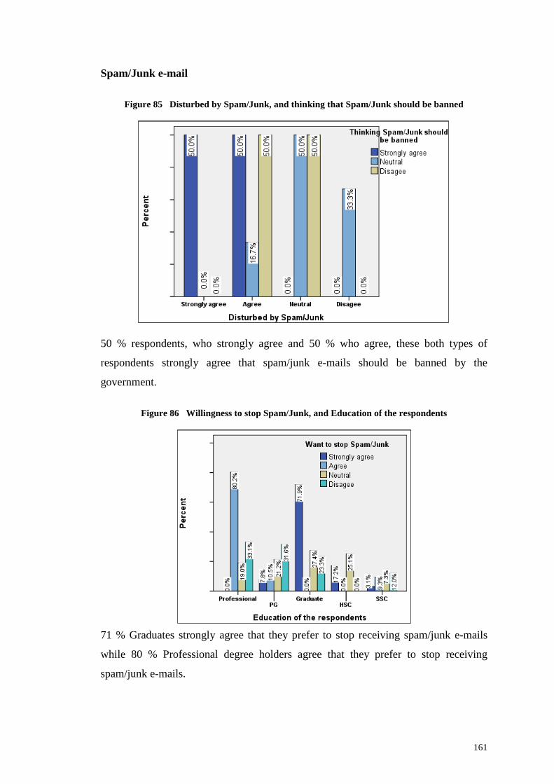
161
Spam/Junk e-mail
Figure 85 Disturbed by Spam/Junk, and thinking that Spam/Junk should be banned
50 % respondents, who strongly agree and 50 % who agree, these both types of
respondents strongly agree that spam/junk e-mails should be banned by the
government.
Figure 86 Willingness to stop Spam/Junk, and Education of the respondents
71 % Graduates strongly agree that they prefer to stop receiving spam/junk e-mails
while 80 % Professional degree holders agree that they prefer to stop receiving
spam/junk e-mails.
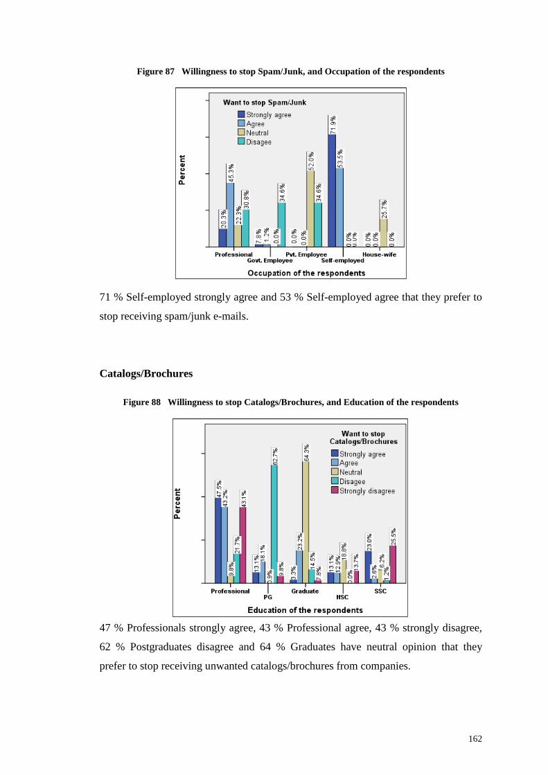
162
Figure 87 Willingness to stop Spam/Junk, and Occupation of the respondents
71 % Self-employed strongly agree and 53 % Self-employed agree that they prefer to
stop receiving spam/junk e-mails.
Catalogs/Brochures
Figure 88 Willingness to stop Catalogs/Brochures, and Education of the respondents
47 % Professionals strongly agree, 43 % Professional agree, 43 % strongly disagree,
62 % Postgraduates disagree and 64 % Graduates have neutral opinion that they
prefer to stop receiving unwanted catalogs/brochures from companies.
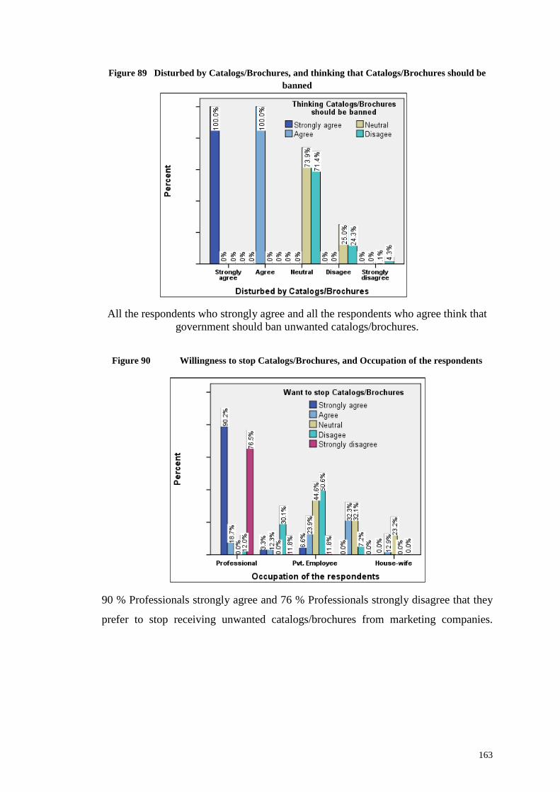
163
Figure 89 Disturbed by Catalogs/Brochures, and thinking that Catalogs/Brochures should be
banned
All the respondents who strongly agree and all the respondents who agree think thatgovernment should ban unwanted catalogs/brochures.
Figure 90 Willingness to stop Catalogs/Brochures, and Occupation of the respondents
90 % Professionals strongly agree and 76 % Professionals strongly disagree that they
prefer to stop receiving unwanted catalogs/brochures from marketing companies.
164
Chapter Bibliography
Books
1. Argyrous George, Statistics for Research: With a Guide to SPSS, Sage
Publications Ltd, 2nd ed, 2005.
2. Belle Gerald Van, Statistics Rules of Thumb¸ 1st ed, Wiley-Interscience, 2002.
3. Field Andy, Discovering Statistics Using SPSS for Windows: Advanced
Techniques for the Beginner, Sage Publications Ltd, 1st ed 2000.
4. Kerr Alistair, Hall Howard and Kozub Stephen, Doing Statistics with SPSS,
SAGE Publications Ltd, 2002.
5. Nargundkar Rajendra, Marketing Research: Text & Cases, 2nd ed, Tata McGraw-
Hill, 2003.
6. Rao A Sajeevan and Tyagi Deepak, Research Methodology with SPSS: Statistical
Package for the Social Sciences, 1st ed, Shree Niwas Publications, Jaipur, 2009.
Websites
1. www.etstrategicmarketing.com, Accessed on Aug 9, 2007
2. www.ezlistmailer.com/images/downloads/EZL-hite-Paper-December-
2006.doc+permission+marketing&hl=en&ct=clnk&cd=5&gl=in, Accessed on
Aug 9, 2007