chapter 5 - field soil water regime - department of land...
TRANSCRIPT

Soil Physics 107, Chapter 5 Page 5-1
Chapter 5 - Field Soil Water Regime
• Infiltration• Redistribution and drainage• Evaporation
Infiltration
Definition: Entry of water into soil through the soil surface.
Also, infiltration is typically not steady state, but infiltration rate, water content or h will all change with time.
In practice: Fraction of water that is applied to the soil surface (rainfall, irrigation), that is notdirectly intercepted by plant cover or is redirected across the soil surface by runoff.
Ponded soil surface θi θo
Water contentSaturation Zone
Transmission Zone
Wetting Zone Wetting Front
As water infiltrates into the soil, the length of the transmission zone increases, andthe infiltrating water wets the soil’s wetting zone, which subsequently moves down in the soilprofile.
Soil Physics 107, Chapter 5 Page 5-2
Notation:
θi Initial volumetric water content (before wetting)
θo Volumetric water content at wetting (at or close to saturation)
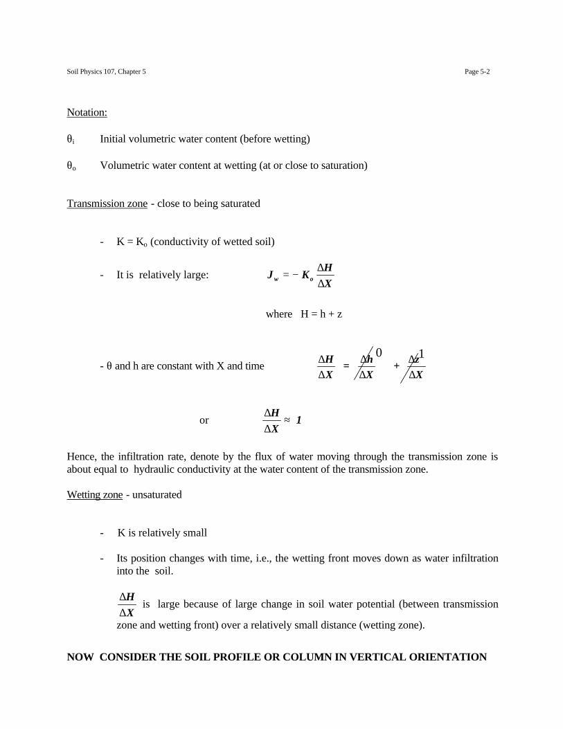
Transmission zone - close to being saturated
- K = Ko (conductivity of wetted soil)
- It is relatively large: J KHXw o= −
∆∆
where H = h + z
- θ and h are constant with X and time ∆∆
∆∆
∆∆
HX
= hX
+ zX
0 1
or ∆∆
HX
1≈
Hence, the infiltration rate, denote by the flux of water moving through the transmission zone isabout equal to hydraulic conductivity at the water content of the transmission zone.
Wetting zone - unsaturated
- K is relatively small
- Its position changes with time, i.e., the wetting front moves down as water infiltrationinto the soil.
∆∆
HX
is large because of large change in soil water potential (between transmission
zone and wetting front) over a relatively small distance (wetting zone).
NOW CONSIDER THE SOIL PROFILE OR COLUMN IN VERTICAL ORIENTATION
Soil Physics 107, Chapter 5 Page 5-3
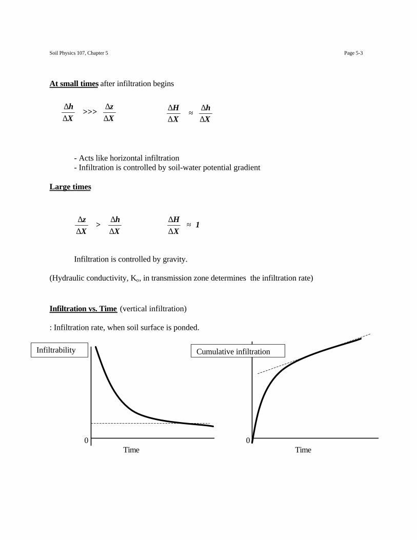
At small times after infiltration begins
- Acts like horizontal infiltration- Infiltration is controlled by soil-water potential gradient
Large times
∆∆
∆∆
zX
> hX
∆∆
HX
1≈
Infiltration is controlled by gravity.
(Hydraulic conductivity, Ko, in transmission zone determines the infiltration rate)
Infiltration vs. Time (vertical infiltration)
: Infiltration rate, when soil surface is ponded.
0 0Time Time
Cumulative infiltrationInfiltrability
∆∆
∆∆
hX
>>> zX
∆∆
∆∆
HX
hX
≈
Soil Physics 107, Chapter 5 Page 5-4
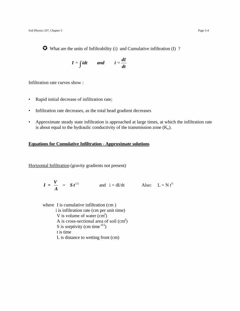
J What are the units of Infiltrability (i) and Cumulative infiltration (I) ?
I idt and idIdt
= =∫
Infiltration rate curves show :
• Rapid initial decrease of infiltration rate;
• Infiltration rate decreases, as the total head gradient decreases
• Approximate steady state infiltration is approached at large times, at which the infiltration rateis about equal to the hydraulic conductivity of the transmission zone (Ko).
Equations for Cumulative Infiltration - Approximate solutions
Horizontal Infiltration (gravity gradients not present)
I = VA
S t= 1 2/ and i = dI/dt Also: L = N t½
where I is cumulative infiltration (cm ) i is infiltration rate (cm per unit time)
V is volume of water (cm3)A is cross-sectional area of soil (cm2)S is sorptivity (cm time -0.5)t is timeL is distance to wetting front (cm)
Soil Physics 107, Chapter 5 Page 5-5
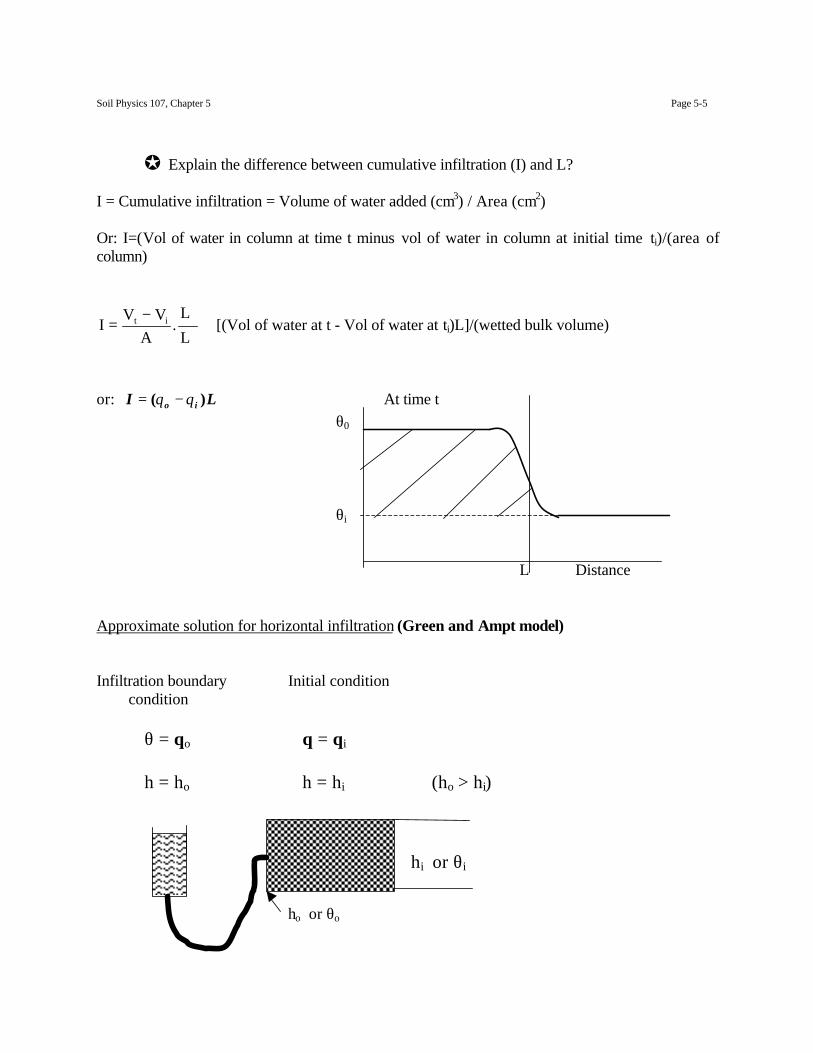
J Explain the difference between cumulative infiltration (I) and L?
I = Cumulative infiltration = Volume of water added (cm3) / Area (cm2)
Or: I=(Vol of water in column at time t minus vol of water in column at initial time ti)/(area ofcolumn)
L
L.
AVV
I it −= [(Vol of water at t - Vol of water at ti)L]/(wetted bulk volume)
or: I Lo i= −( )θ θ At time tθ0
θi
L Distance
Approximate solution for horizontal infiltration (Green and Ampt model)
Infiltration boundary Initial condition condition
θ = θo θ = θi
h = ho h = hi (ho > hi)
ho or θo
hi or θi
Soil Physics 107, Chapter 5 Page 5-6
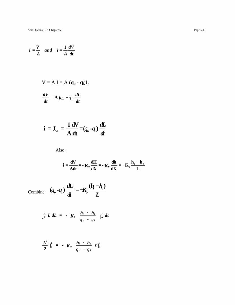
IVA
and iA
dVdt
= =1
V = A I = A (θo - θi)L
dVdt
dLdti= − )A (θ θο
dLdt
i = J = 1A
dVdt
=( - ) w o iθ θ
Also:
Combine: dLdt
Kh h
Loi o ( - ) o iθ θ =−−( )
0L
oi o
o iot L dL = - K h - h
- dt∫
∫
θ θ
2
0L
oi o
o iotL
2 | = - K h - h
- t |
θ θ
Lhh
KdXdh
K - = dXdH K - =
AdtdV
i oiooo
−−==
Soil Physics 107, Chapter 5 Page 5-7
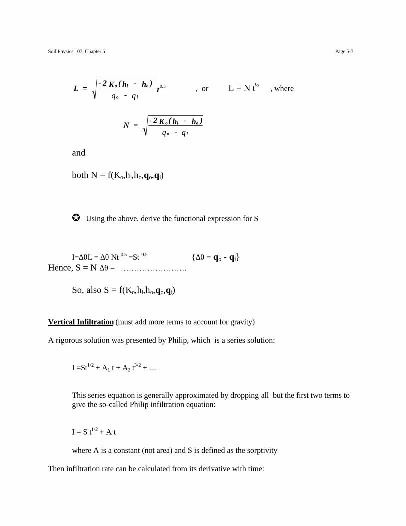
L = - 2 K ( h - h )
- to i o
o iθ θ0 5. , or L = N t½ , where
and
both N = f(Ko,hi,ho,θo,θi)
J Using the above, derive the functional expression for S
I=∆θL = ∆θ Nt 0.5 =St 0.5 {∆θ = θo - θi}Hence, S = N ∆θ = …………………….
So, also S = f(Ko,hi,ho,θo,θi)
Vertical Infiltration (must add more terms to account for gravity)
A rigorous solution was presented by Philip, which is a series solution:
I =St1/2 + A1 t + A2 t3/2 + ....
This series equation is generally approximated by dropping all but the first two terms togive the so-called Philip infiltration equation:
I = S t1/2 + A t
where A is a constant (not area) and S is defined as the sorptivity Then infiltration rate can be calculated from its derivative with time:
N = - 2 K ( h - h ) -
o i o
o iθ θ
Soil Physics 107, Chapter 5 Page 5-8
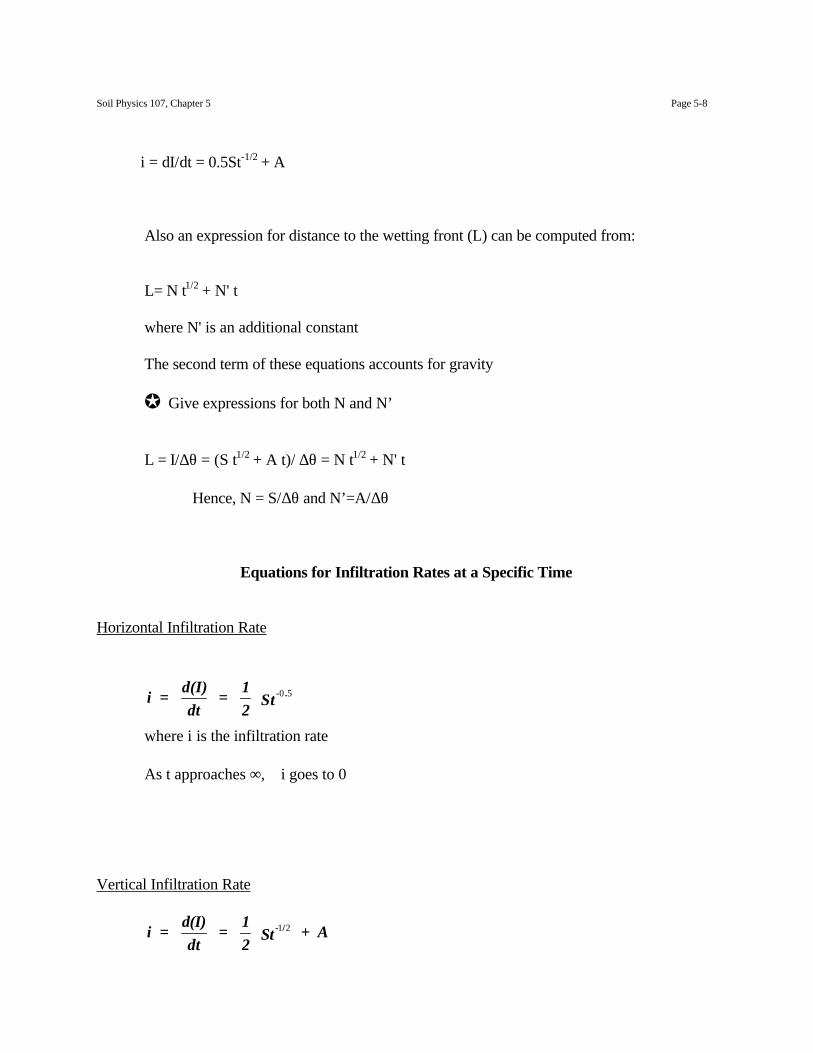
i = dI/dt = 0.5St-1/2 + A
Also an expression for distance to the wetting front (L) can be computed from:
L= N t1/2 + N' t
where N' is an additional constant
The second term of these equations accounts for gravity
J Give expressions for both N and N’
L = I/∆θ = (S t1/2 + A t)/ ∆θ = N t1/2 + N' t
Hence, N = S/∆θ and N’=A/∆θ
Equations for Infiltration Rates at a Specific Time
Horizontal Infiltration Rate
i = d(I)dt
= 12
St -0 5.
where i is the infiltration rate
As t approaches ∞, i goes to 0
Vertical Infiltration Rate
i = d(I)dt
= 12
St + A-1 2/
Soil Physics 107, Chapter 5 Page 5-9
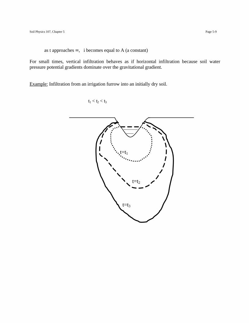
as t approaches ∞, i becomes equal to A (a constant)
For small times, vertical infiltration behaves as if horizontal infiltration because soil waterpressure potential gradients dominate over the gravitational gradient.
Example: Infiltration from an irrigation furrow into an initially dry soil.
t1 < t2 < t3
t=t1
t=t2
t=t3
Soil Physics 107, Chapter 5 Page 5-10
Effect of Soil Properties on Infiltration
1. Effects of soil moisture, texture and layering:
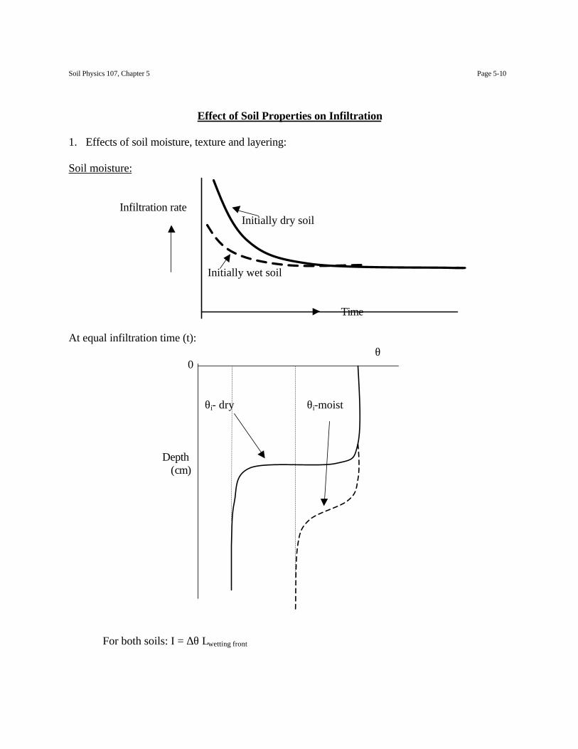
Soil moisture:
Infiltration rate Initially dry soil
Initially wet soil
Time
At equal infiltration time (t):θ
0
θi- dry θi-moist
Depth (cm)
For both soils: I = ∆θ Lwetting front
Soil Physics 107, Chapter 5 Page 5-11
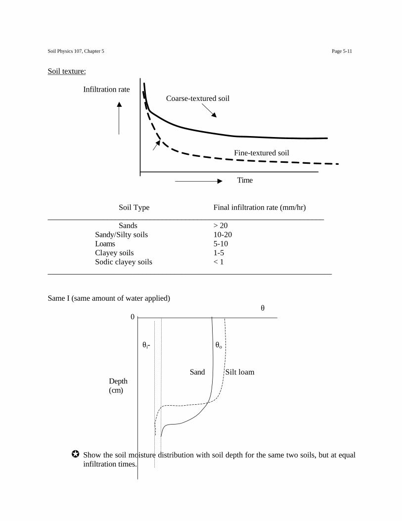
Soil texture:
Infiltration rateCoarse-textured soil
Fine-textured soil
Time
Soil Type Final infiltration rate (mm/hr)______________________________________________________________________
Sands > 20Sandy/Silty soils 10-20Loams 5-10Clayey soils 1-5Sodic clayey soils < 1
________________________________________________________________________
Same I (same amount of water applied)θ
0
θi- θo
Sand Silt loam Depth (cm)
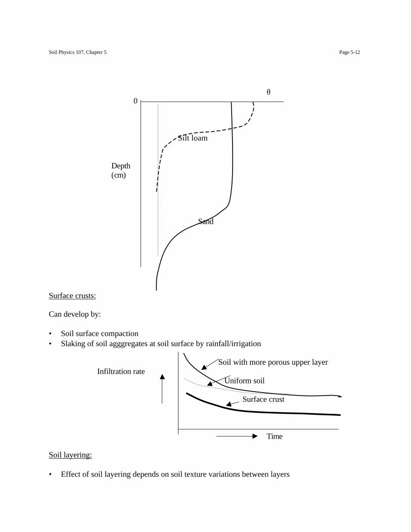
J Show the soil moisture distribution with soil depth for the same two soils, but at equalinfiltration times.
Soil Physics 107, Chapter 5 Page 5-12
θ 0
Silt loam
Depth (cm)
Sand
Surface crusts:
Can develop by:
• Soil surface compaction• Slaking of soil agggregates at soil surface by rainfall/irrigation
Soil with more porous upper layerInfiltration rate
Uniform soil
Surface crust
Time
Soil layering:
• Effect of soil layering depends on soil texture variations between layers
Soil Physics 107, Chapter 5 Page 5-13
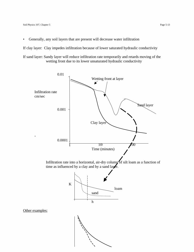
• Generally, any soil layers that are present will decrease water infiltration
If clay layer: Clay impedes infiltration because of lower saturated hydraulic conductivity
If sand layer: Sandy layer will reduce infiltration rate temporarily and retards moving of thewetting front due to its lower unsaturated hydraulic conductivity
0.01Wetting front at layer
Infiltration ratecm/sec
Sand layer0.001
Clay layer
-0.0001
1 10 100Time (minutes)
Infiltration rate into a horizontal, air-dry column of silt loam as a function oftime as influenced by a clay and by a sand layer.
Kloam
sand
h
Other examples:
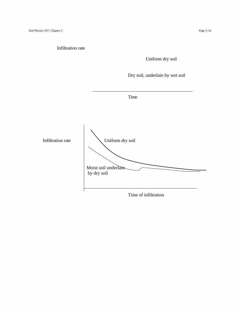
Soil Physics 107, Chapter 5 Page 5-14
Infiltration rate
Uniform dry soil
Dry soil, underlain by wet soil
Time
Infiltration rate Uniform dry soil
Moist soil underlain by dry soil
Time of infiltration
Soil Physics 107, Chapter 5 Page 5-15
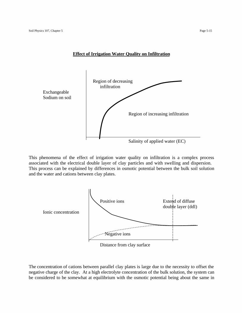
Effect of Irrigation Water Quality on Infiltration
Region of decreasinginfiltration
ExchangeableSodium on soil
Region of increasing infiltration
Salinity of applied water (EC)
This phenomena of the effect of irrigation water quality on infiltration is a complex processassociated with the electrical double layer of clay particles and with swelling and dispersion. This process can be explained by differences in osmotic potential between the bulk soil solutionand the water and cations between clay plates.
Positive ions Extend of diffuse double layer (ddl)
Ionic concentration
Negative ions
Distance from clay surface
The concentration of cations between parallel clay plates is large due to the necessity to offset thenegative charge of the clay. At a high electrolyte concentration of the bulk solution, the system canbe considered to be somewhat at equilibrium with the osmotic potential being about the same in
Soil Physics 107, Chapter 5 Page 5-16
the solution between the clay plates and the bulk solution. When the bulk solution electrolyteconcentration is dropped drastically by adding pure water, an osmotic potential gradient is set upbetween the bulk solution and that between the clay plates. Thus, water moves from the bulksolution to the area between the clay plates causing the plates to be pushed apart or the soil toswell. This swelling decreases the volume of pores through which infiltration occurs and thusdecreases infiltration rate. If a large amount of water is imbibed between clay particles, some ofthe particles may break away and move with the infiltrating water until a constriction is reachedcausing plugging of the pores.
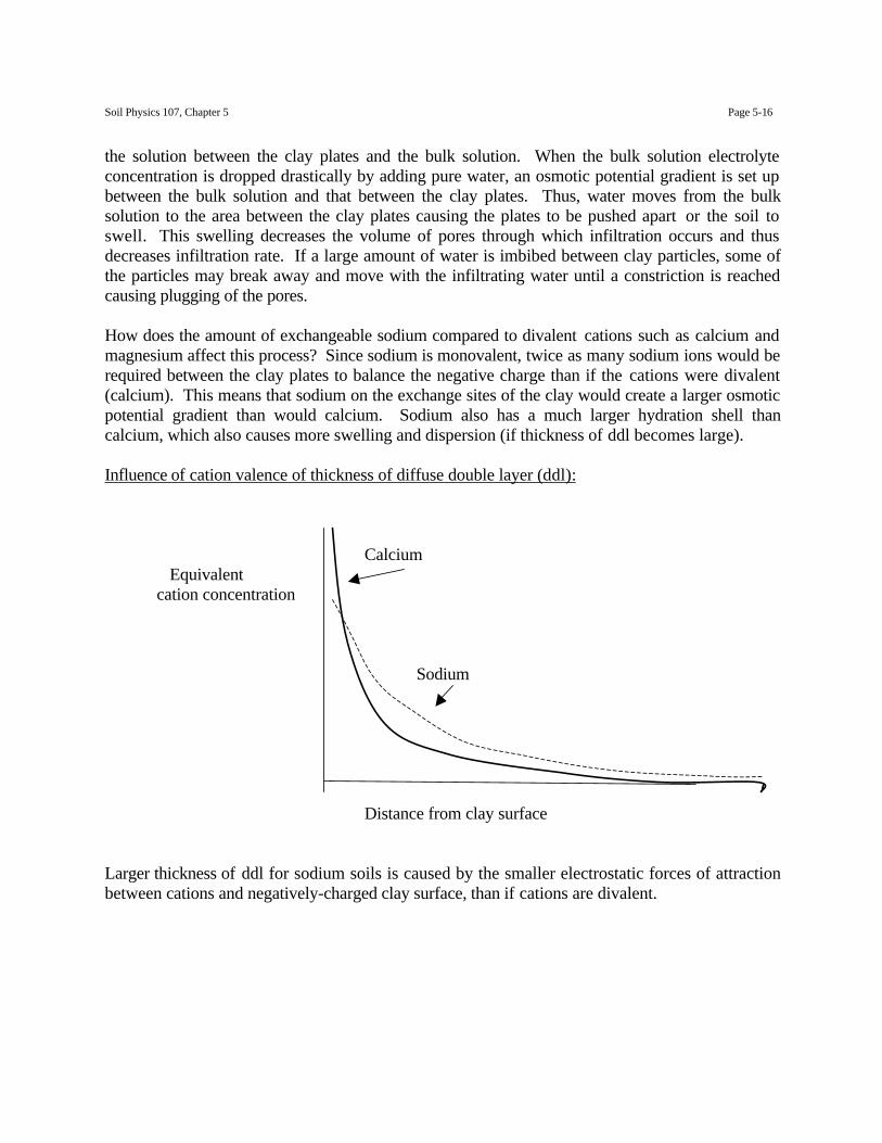
How does the amount of exchangeable sodium compared to divalent cations such as calcium andmagnesium affect this process? Since sodium is monovalent, twice as many sodium ions would berequired between the clay plates to balance the negative charge than if the cations were divalent(calcium). This means that sodium on the exchange sites of the clay would create a larger osmoticpotential gradient than would calcium. Sodium also has a much larger hydration shell thancalcium, which also causes more swelling and dispersion (if thickness of ddl becomes large).
Influence of cation valence of thickness of diffuse double layer (ddl):
Calcium Equivalentcation concentration
Sodium
Distance from clay surface
Larger thickness of ddl for sodium soils is caused by the smaller electrostatic forces of attractionbetween cations and negatively-charged clay surface, than if cations are divalent.
Soil Physics 107, Chapter 5 Page 5-17
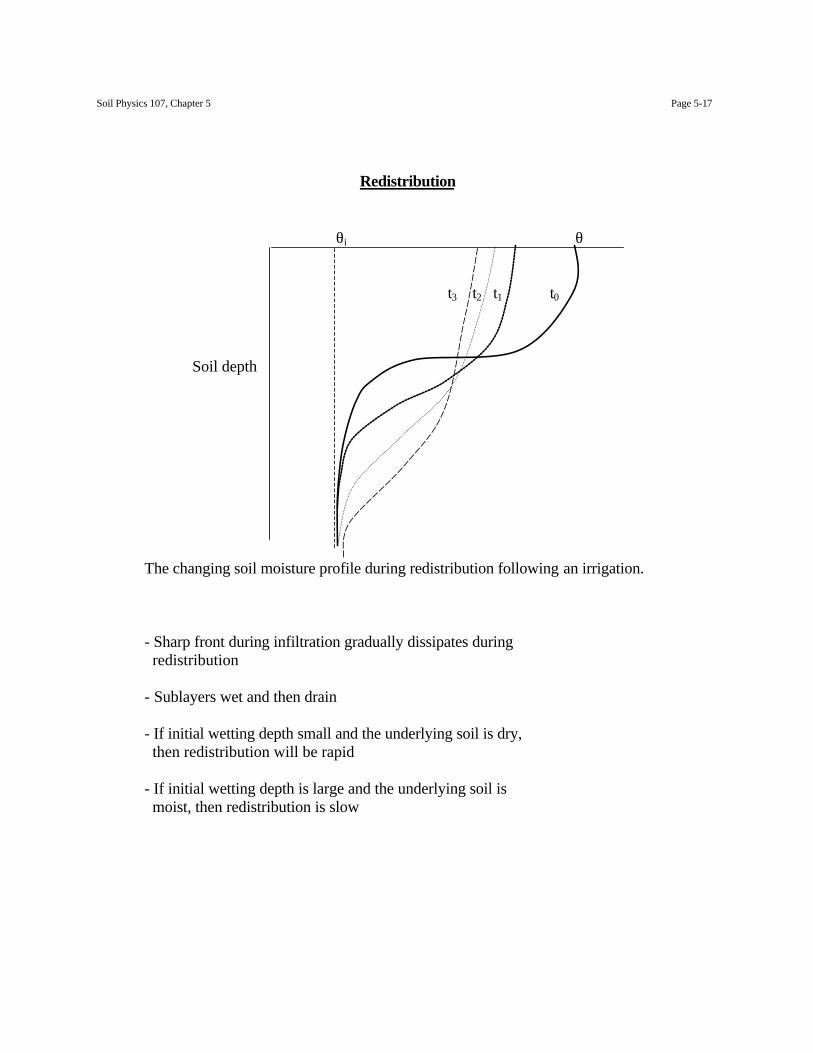
Redistribution
θi θ
t3 t2 t1 t0
Soil depth
The changing soil moisture profile during redistribution following an irrigation.
- Sharp front during infiltration gradually dissipates during redistribution
- Sublayers wet and then drain
- If initial wetting depth small and the underlying soil is dry, then redistribution will be rapid
- If initial wetting depth is large and the underlying soil is moist, then redistribution is slow
Soil Physics 107, Chapter 5 Page 5-18
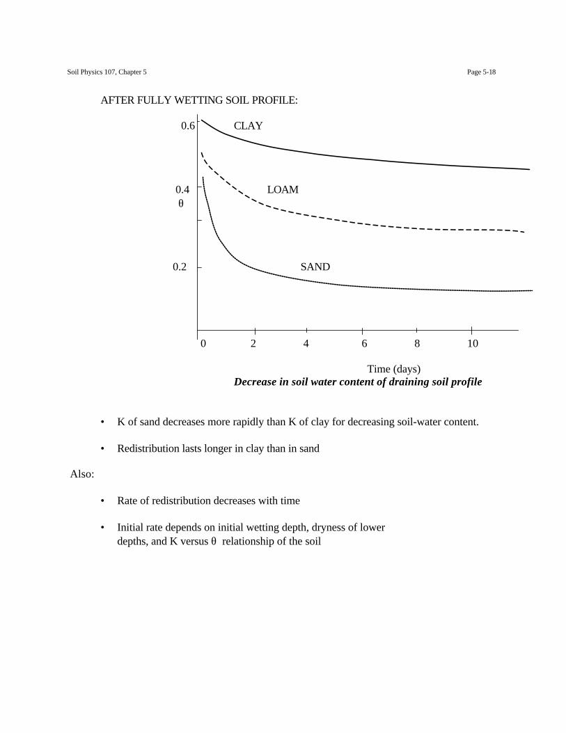
AFTER FULLY WETTING SOIL PROFILE:
0.6 CLAY
0.4 LOAM θ
0.2 SAND
0 2 4 6 8 10
Time (days)Decrease in soil water content of draining soil profile
• K of sand decreases more rapidly than K of clay for decreasing soil-water content.
• Redistribution lasts longer in clay than in sand
Also:
• Rate of redistribution decreases with time
• Initial rate depends on initial wetting depth, dryness of lower depths, and K versus θ relationship of the soil
Soil Physics 107, Chapter 5 Page 5-19
Decrease of redistribution with time is caused by:
1. ∆∆
hX
decreases with time as wet zone loses water and dry zone gains water
2. K decreases with time as wet zone θ decreases, so both ∆∆
HX
and K are decreasing with time.
Therefore, Jw (redistribution rate) is decreasing with time as well
Also, redistribution results in drying of the surface soil and wetting of the subsurface soil:
- Soil is both wetting and drying (hysteresis)
- θ versus h becomes complicated
- Net effect of simultaneously wetting and drying within soil profile is to retard water redistribution
Soil Physics 107, Chapter 5 Page 5-20
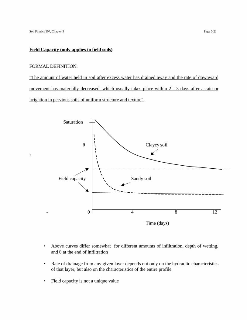
Field Capacity (only applies to field soils)
FORMAL DEFINITION:
"The amount of water held in soil after excess water has drained away and the rate of downward
movement has materially decreased, which usually takes place within 2 - 3 days after a rain or
irrigation in pervious soils of uniform structure and texture".
Saturation
θ Clayey soil
‘
Field capacity Sandy soil
- 0 4 8 12
Time (days)
• Above curves differ somewhat for different amounts of infiltration, depth of wetting,and θ at the end of infiltration
• Rate of drainage from any given layer depends not only on the hydraulic characteristicsof that layer, but also on the characteristics of the entire profile
• Field capacity is not a unique value
Soil Physics 107, Chapter 5 Page 5-21
Factors affecting field capacity
1. Texture
The finer the texture of the soil particles, the higher is the apparent field capacity and theslower it is attained. Also its value will be less distinct
= 0.04 sandsField capacity
= 0.45 clay
2. Type of Clay
Soils high in montmorillonite have higher field capacity values
3. Organic Matter
Increases field capacity (as high as 100% in organic soils)
4. Depth of initial wetting
In general (but not always),
The wetter the lower soil profile at the beginning of redistribution, and the greater the depth ofwetting, the slower the rate of redistribution, and the greater the value of field capacity
5. Impeding layers
Inhibit redistribution and increase field capacity
6. Evapotranspiration
Modifies redistribution and affects field capacity
J How will evaporation affect field capacity?
Redistribution - mathematical solution
Soil Physics 107, Chapter 5 Page 5-22
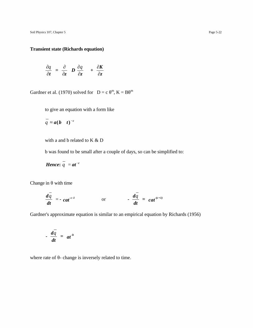
Transient state (Richards equation)
∂∂
∂∂
∂∂
∂∂
θ θt
= z
D z
+ Kz
Gardner et al. (1970) solved for D = c θm, K = Bθm
to give an equation with a form like
θ ≈ + −a b t c( )
with a and b related to K & D
b was found to be small after a couple of days, so can be simplified to:
Hence at c: θ = −
Change in θ with time
ddt
- cat-c-1θ= or -
ddt
cat-(c+1)θ=
Gardner's approximate equation is similar to an empirical equation by Richards (1956)
- ddt
= at -bθ
where rate of θ- change is inversely related to time.
Soil Physics 107, Chapter 5 Page 5-23
Evaporation - Bare Surface Soil
• Removal of water from the soil by evaporation.
• 3 conditions are necessary for evaporation to occur
1. Heat supply - 590 cal/g or 2500 J/g H2O
2. Vapor pressure gradient between soil and air
3. Supply of H2O from underlying soil to surface
• Evaporation situtations considered here are:
1. Situations of shallow groundwater (may be steady flow)
2. Situations of deep water table (transient flow)
3. One-dimensional and 2- or 3-dimensional flow (cracks)
4. Environmental conditions constant or fluctuating
1. Steady state evaporation, with a shallow water table (capillary rise)
• Upward flow possible because of capillary rise from water table
• Water moves upward from water table into initially dry soil because of total soil waterpotential decreasing upwards.
• Rate of upward water movement decreases with time, as the total water potential gradientapproaches zero.
at t infinity, Hz
= 0, and h = - z→∆∆
(if reference level at water table)
Soil Physics 107, Chapter 5 Page 5-24
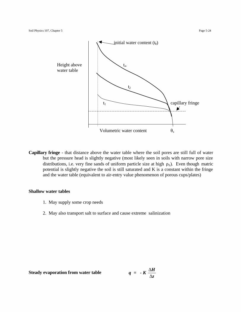
initial water content (t0)
Height above t∞water table
t2
t1 capillary fringe
Volumetric water content θs
Capillary fringe - that distance above the water table where the soil pores are still full of waterbut the pressure head is slightly negative (most likely seen in soils with narrow pore sizedistributions, i.e. very fine sands of uniform particle size at high ρb). Even though matricpotential is slightly negative the soil is still saturated and K is a constant within the fringeand the water table (equivalent to air-entry value phenomenon of porous cups/plates)
Shallow water tables
1. May supply some crop needs
2. May also transport salt to surface and cause extreme salinization
Steady evaporation from water table q = - K Hz
∆∆
Soil Physics 107, Chapter 5 Page 5-25
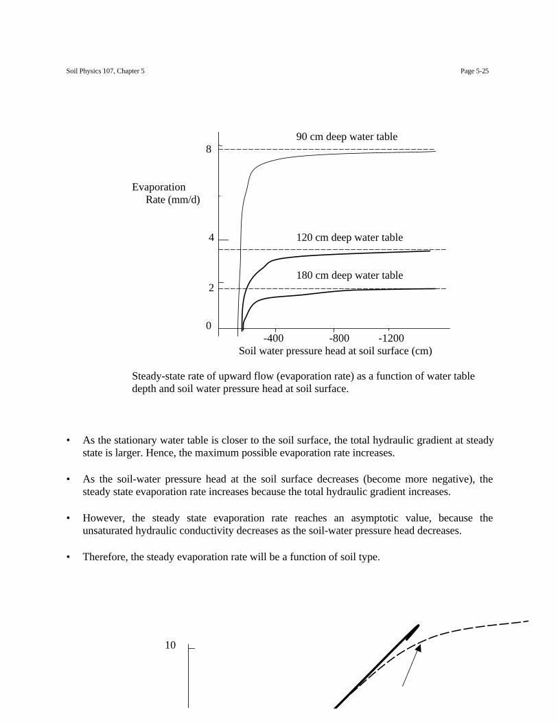
90 cm deep water table 8
Evaporation Rate (mm/d)
4 120 cm deep water table
180 cm deep water table 2
0-400 -800 -1200
Soil water pressure head at soil surface (cm)
Steady-state rate of upward flow (evaporation rate) as a function of water tabledepth and soil water pressure head at soil surface.
• As the stationary water table is closer to the soil surface, the total hydraulic gradient at steadystate is larger. Hence, the maximum possible evaporation rate increases.
• As the soil-water pressure head at the soil surface decreases (become more negative), thesteady state evaporation rate increases because the total hydraulic gradient increases.
• However, the steady state evaporation rate reaches an asymptotic value, because theunsaturated hydraulic conductivity decreases as the soil-water pressure head decreases.
• Therefore, the steady evaporation rate will be a function of soil type.
10
Soil Physics 107, Chapter 5 Page 5-26
1:1-line
Fine-textured soil
Evaporationrate (mm/d) 5
Coarse-textured soil
0 10 15
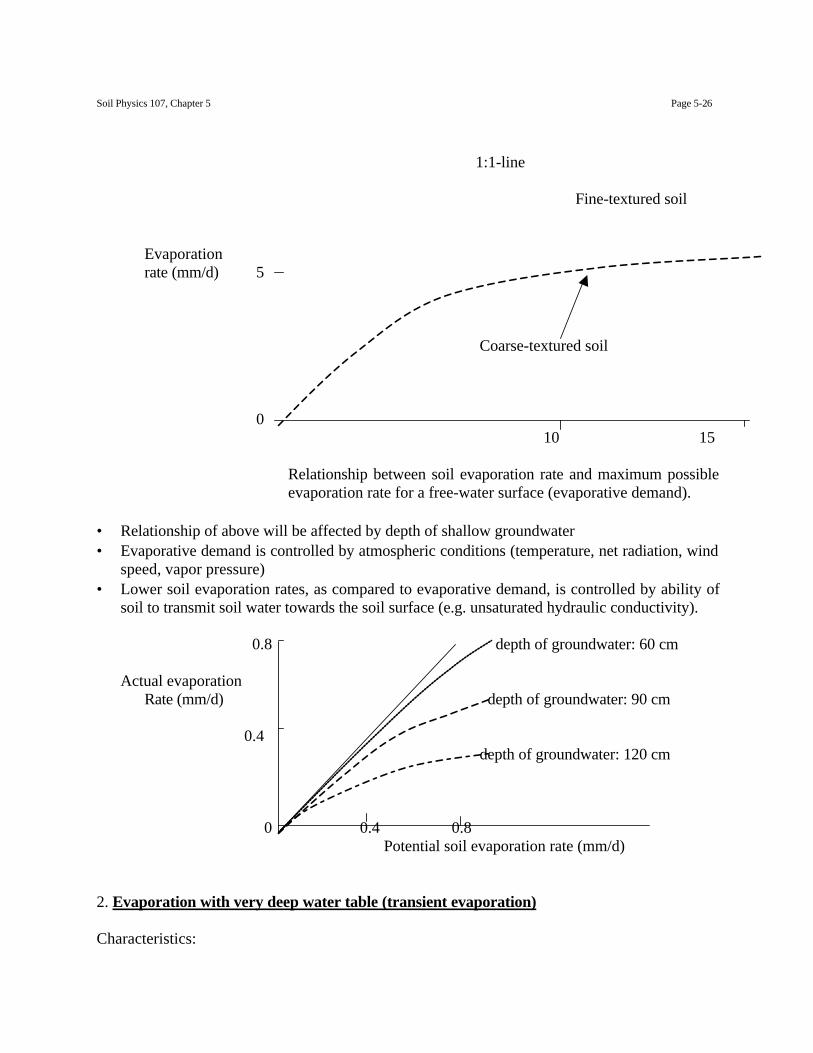
Relationship between soil evaporation rate and maximum possibleevaporation rate for a free-water surface (evaporative demand).
• Relationship of above will be affected by depth of shallow groundwater• Evaporative demand is controlled by atmospheric conditions (temperature, net radiation, wind
speed, vapor pressure)• Lower soil evaporation rates, as compared to evaporative demand, is controlled by ability of
soil to transmit soil water towards the soil surface (e.g. unsaturated hydraulic conductivity).
0.8 depth of groundwater: 60 cm
Actual evaporationRate (mm/d) depth of groundwater: 90 cm
0.4depth of groundwater: 120 cm
0 0.4 0.8Potential soil evaporation rate (mm/d)
2. Evaporation with very deep water table (transient evaporation)
Characteristics:
Soil Physics 107, Chapter 5 Page 5-27
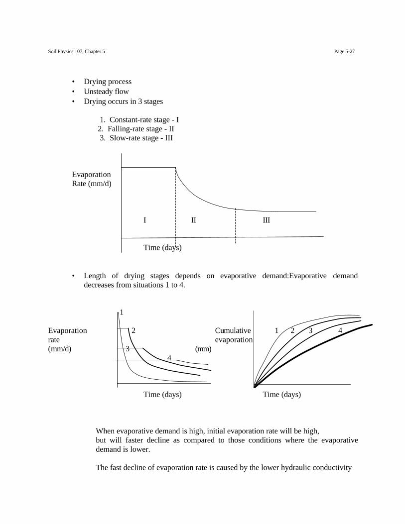
• Drying process• Unsteady flow• Drying occurs in 3 stages
1. Constant-rate stage - I 2. Falling-rate stage - II
3. Slow-rate stage - III
EvaporationRate (mm/d)
I II III
Time (days)
• Length of drying stages depends on evaporative demand:Evaporative demanddecreases from situations 1 to 4.
1
Evaporation 2 Cumulative 1 2 3 4rate evaporation(mm/d) 3 (mm)
4
Time (days) Time (days)
When evaporative demand is high, initial evaporation rate will be high,but will faster decline as compared to those conditions where the evaporativedemand is lower.
The fast decline of evaporation rate is caused by the lower hydraulic conductivity
Soil Physics 107, Chapter 5 Page 5-28
of the soil as the near soil decreases in water content.
However, given it enough time, all curves will eventually approach the sameamount of cumulative evaporation (mm).
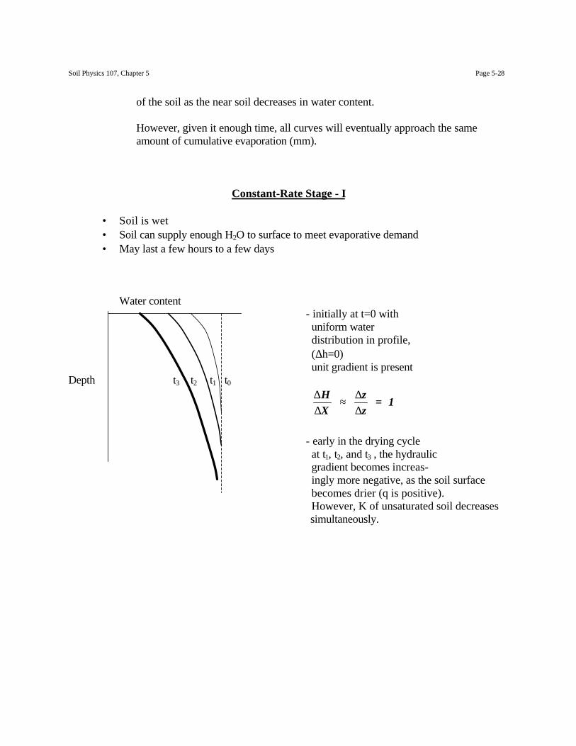
Constant-Rate Stage - I
• Soil is wet• Soil can supply enough H2O to surface to meet evaporative demand• May last a few hours to a few days
Water content- initially at t=0 with uniform water distribution in profile, (∆h=0) unit gradient is present
Depth t3 t2 t1 t0∆∆
∆∆
HX
zz
= 1≈
- early in the drying cycle at t1, t2, and t3 , the hydraulic gradient becomes increas- ingly more negative, as the soil surface becomes drier (q is positive). However, K of unsaturated soil decreases simultaneously.
Soil Physics 107, Chapter 5 Page 5-29
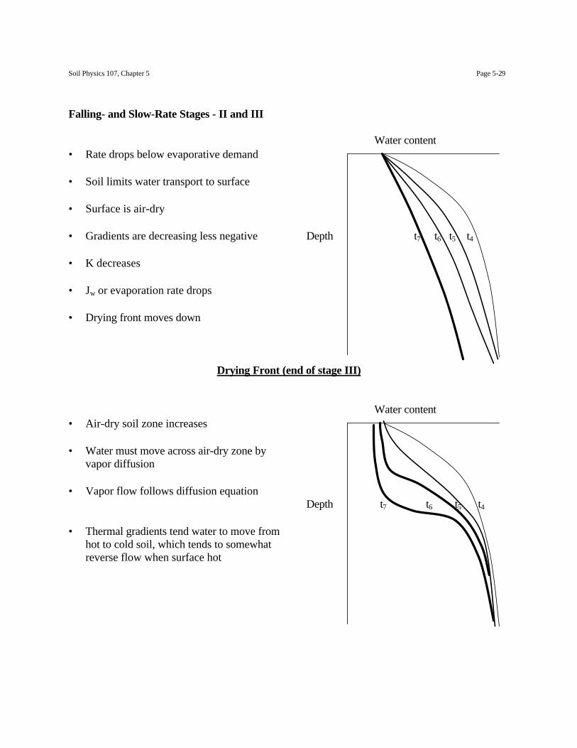
Falling- and Slow-Rate Stages - II and III
Water content• Rate drops below evaporative demand
• Soil limits water transport to surface
• Surface is air-dry
• Gradients are decreasing less negative Depth t7 t6 t5 t4
• K decreases
• Jw or evaporation rate drops
• Drying front moves down
Drying Front (end of stage III)
Water content• Air-dry soil zone increases
• Water must move across air-dry zone byvapor diffusion
• Vapor flow follows diffusion equation Depth t7 t6 t5 t4
• Thermal gradients tend water to move from hot to cold soil, which tends to somewhat reverse flow when surface hot
Soil Physics 107, Chapter 5 Page 5-30
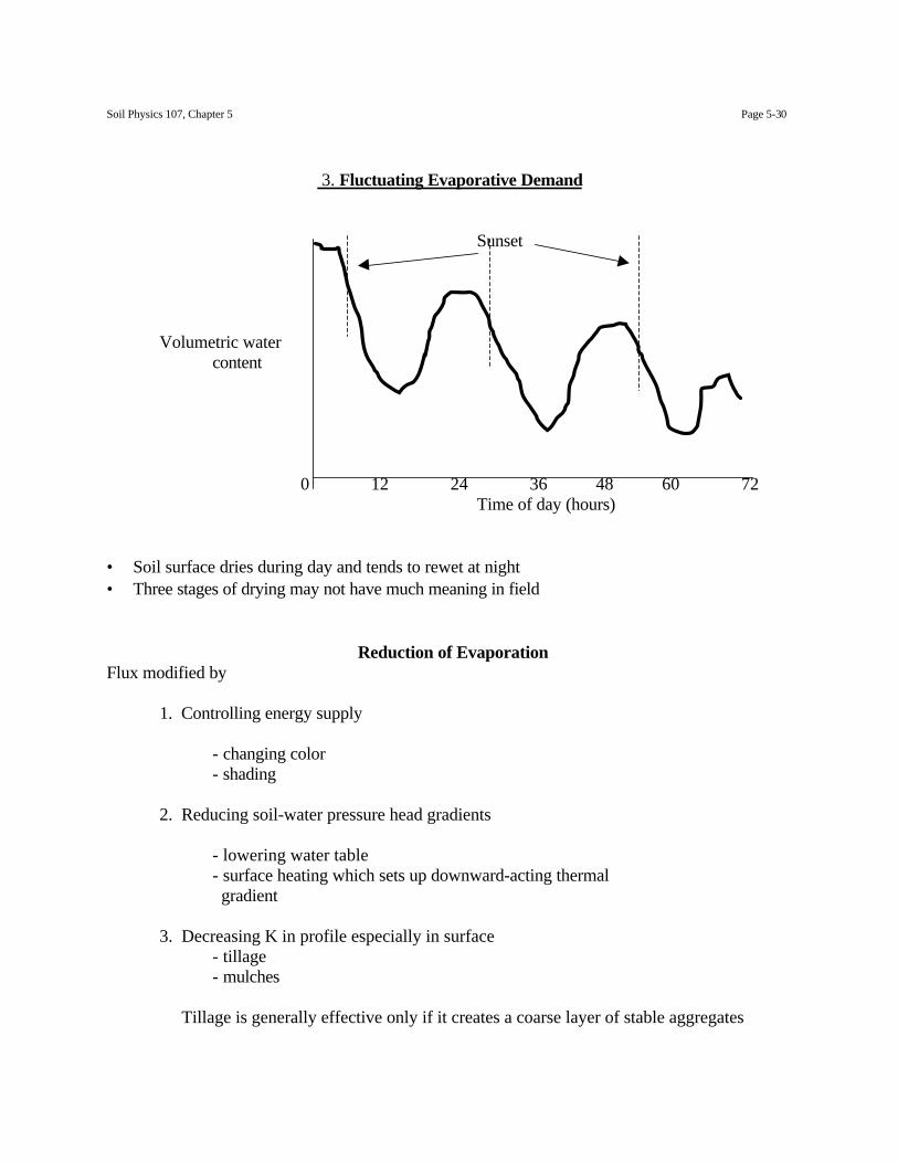
3. Fluctuating Evaporative Demand
Sunset
Volumetric watercontent
0 12 24 36 48 60 72Time of day (hours)
• Soil surface dries during day and tends to rewet at night• Three stages of drying may not have much meaning in field
Reduction of EvaporationFlux modified by
1. Controlling energy supply
- changing color- shading
2. Reducing soil-water pressure head gradients
- lowering water table- surface heating which sets up downward-acting thermal gradient
3. Decreasing K in profile especially in surface- tillage- mulches
Tillage is generally effective only if it creates a coarse layer of stable aggregates