Chapter 5 - AnnuitiesSection 5.3 - Review of Annuities-Certain

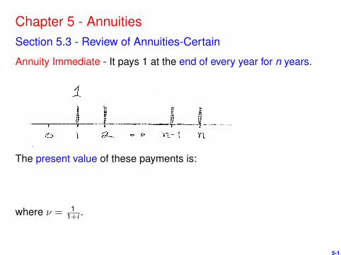
Annuity Immediate - It pays 1 at the end of every year for n years.

The present value of these payments is:

where ν = 11+i .

5-1

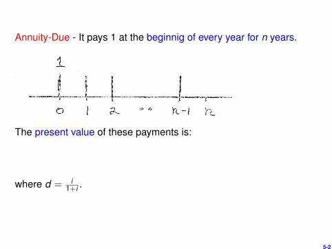
Annuity-Due - It pays 1 at the beginnig of every year for n years.

The present value of these payments is:

where d = i1+i .

5-2

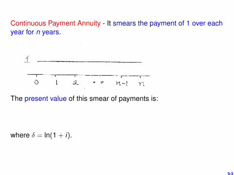
Continuous Payment Annuity - It smears the payment of 1 over eachyear for n years.

The present value of this smear of payments is:

where δ = ln(1 + i).

5-3

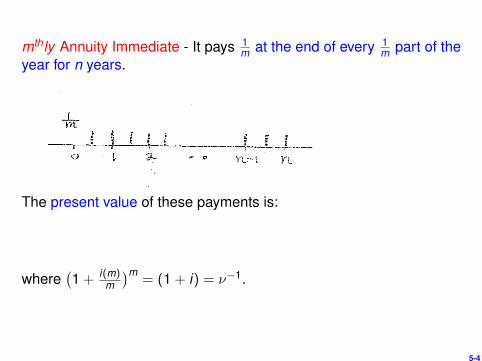
mthly Annuity Immediate - It pays 1m at the end of every 1

m part of theyear for n years.

The present value of these payments is:

where(1 + i(m)

m

)m= (1 + i) = ν−1.

5-4

mthly Annuity Due - It pays 1m at the beginning of every 1

m part of theyear for n years.

The present value of these payments is:

where(1− d(m)

m

)−m= (1 + i) = ν−1.

5-5

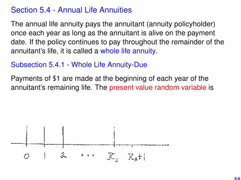
Section 5.4 - Annual Life Annuities

The annual life annuity pays the annuitant (annuity policyholder)once each year as long as the annuitant is alive on the paymentdate. If the policy continues to pay throughout the remainder of theannuitant’s life, it is called a whole life annuity.

Subsection 5.4.1 - Whole Life Annuity-Due

Payments of $1 are made at the beginning of each year of theannuitant’s remaining life. The present value random variable is

5-6

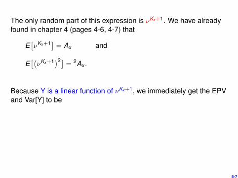
The only random part of this expression is νKx+1. We have alreadyfound in chapter 4 (pages 4-6, 4-7) that

E[νKx+1] = Ax and

E[(νKx+1)2]

= 2Ax .

Because Y is a linear function of νKx+1, we immediately get the EPVand Var[Y] to be

5-7

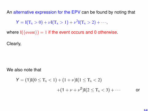
An alternative expression for the EPV can be found by noting that

Y = I(Tx > 0) + νI(Tx > 1) + ν2I(Tx > 2) + · · ·,

where I({event}) = 1 if the event occurs and 0 otherwise.

Clearly,

We also note that

Y = (1)I(0 ≤ Tx < 1) + (1 + ν)I(1 ≤ Tx < 2)

+(1 + ν + ν2)I(2 ≤ Tx < 3) + · · · or

5-8

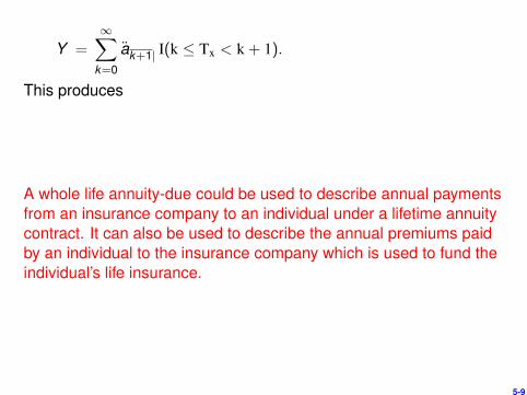
Y =∞∑

k=0

ak+1| I(k ≤ Tx < k + 1).

This produces

A whole life annuity-due could be used to describe annual paymentsfrom an insurance company to an individual under a lifetime annuitycontract. It can also be used to describe the annual premiums paidby an individual to the insurance company which is used to fund theindividual’s life insurance.

5-9

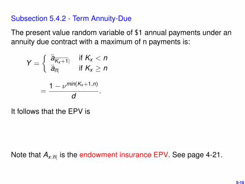
Subsection 5.4.2 - Term Annuity-Due

The present value random variable of $1 annual payments under anannuity due contract with a maximum of n payments is:

Y =

{aKx+1| if Kx < nan| if Kx ≥ n

=1− νmin(Kx+1,n)

d.

It follows that the EPV is

Note that Ax :n| is the endowment insurance EPV. See page 4-21.

5-10

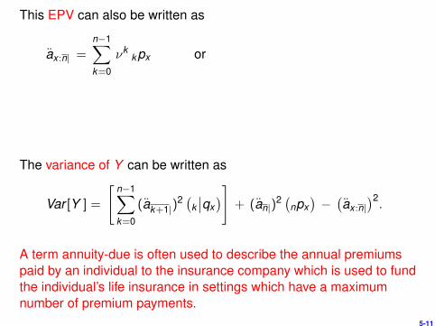
This EPV can also be written as

ax :n| =n−1∑k=0

νkkpx or

The variance of Y can be written as

Var [Y ] =

[n−1∑k=0

(ak+1|)2 (

k∣∣qx)]

+ (an|)2 (

npx)−(ax :n|

)2.

A term annuity-due is often used to describe the annual premiumspaid by an individual to the insurance company which is used to fundthe individual’s life insurance in settings which have a maximumnumber of premium payments.

5-11

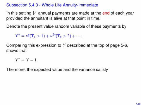
Subsection 5.4.3 - Whole Life Annuity-Immediate

In this setting $1 annual payments are made at the end of each yearprovided the annuitant is alive at that point in time.

Denote the present value random variable of these payments by

Y ∗ = νI(Tx > 1) + ν2I(Tx > 2) + · · ·,

Comparing this expression to Y described at the top of page 5-6,shows that

Y ∗ = Y − 1.

Therefore, the expected value and the variance satisfy

5-12

Subsection 5.4.4 - Term Annuity-Immediate

In this setting the $1 annual payments are made at the end of eachyear provided the annuitant is alive at that point in time, but there willbe at most n payments made. The present value random variable is

Y ∗n = νI(Tx ≥ 1) + ν2I(Tx ≥ 2) + · · ·+ νnI(Tx ≥ n),

= amin(Kx ,n)| =1− νmin(Kx ,n)

i.

It follows that its EPV is

Comparing this to

ax :n| =n−1∑k=0

νk(kpx),

5-13

we see that

Since

Y ∗n =

[n−1∑k=1

ak | I(k ≤ Tx < k + 1)

]+ an|I(Tx ≥ n),

the variance of Y ∗n can be written as

Var [Y ∗n ] =

[n−1∑k=1

(ak |)2 (

k∣∣qx)]

+ (an|)2 (

npx)−(ax :n|

)2.

5-14

Example 5-1: You are given 10p0 = .07, 20p0 = .06 and 30p0 = .04.Suppose each survivor age 20 contributes P to a fund so there is anamount at the end of 10 years to pay $1,000 to each survivor age30. Use i = .06 and find P.

Example 5-2: You are given (1) 10 year pure endowment of 1, (2)whole life annuity-immediate with 1 annual payments, (3) whole lifeannuity-due with 1 annual payments and (4) 10-year temporary lifeannuity-immediate with 1 for annual payments. Rank the actuarialpresent values of these options.

5-15

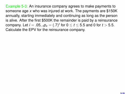
Example 5-3: An insurance company agrees to make payments tosomeone age x who was injured at work. The payments are $150Kannually, starting immediately and continuing as long as the personis alive. After the first $500K the remainder is paid by a reinsurancecompany. Let i = .05, tpx = (.7)t for 0 ≤ t ≤ 5.5 and 0 for t > 5.5.Calculate the EPV for the reinsurance company.

5-16

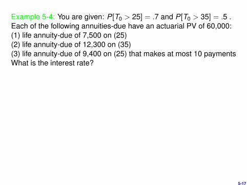
Example 5-4: You are given: P[T0 > 25] = .7 and P[T0 > 35] = .5 .Each of the following annuities-due have an actuarial PV of 60,000:(1) life annuity-due of 7,500 on (25)(2) life annuity-due of 12,300 on (35)(3) life annuity-due of 9,400 on (25) that makes at most 10 paymentsWhat is the interest rate?

5-17

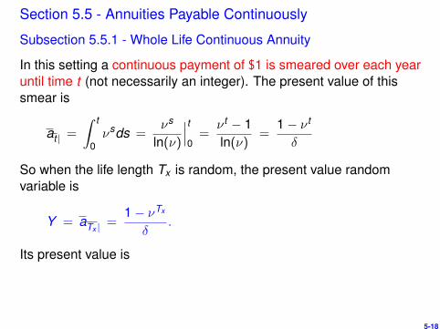
Section 5.5 - Annuities Payable Continuously

Subsection 5.5.1 - Whole Life Continuous Annuity

In this setting a continuous payment of $1 is smeared over each yearuntil time t (not necessarily an integer). The present value of thissmear is

at | =

∫ t

0νsds =

νs

ln(ν)

∣∣∣t0=

ν t − 1ln(ν)

=1− ν t

δ

So when the life length Tx is random, the present value randomvariable is

Y = aTx | =1− νTx

δ.

Its present value is

5-18

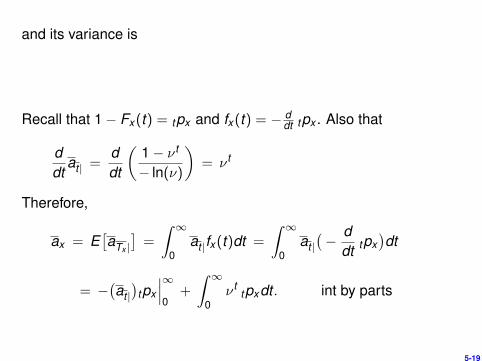
and its variance is

Recall that 1− Fx(t) = tpx and fx(t) = − ddt tpx . Also that

ddt

at | =ddt

(1− ν t

− ln(ν)

)= ν t

Therefore,

ax = E[aTx |

]=

∫ ∞0

at |fx(t)dt =

∫ ∞0

at |(− d

dt tpx)dt

= −(at |)

tpx

∣∣∣∞0

+

∫ ∞0

ν ttpxdt . int by parts

5-19

It follows that

5-20

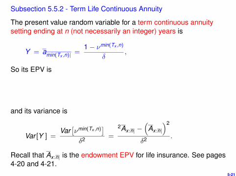
Subsection 5.5.2 - Term Life Continuous Annuity

The present value random variable for a term continuous annuitysetting ending at n (not necessarily an integer) years is

Y = amin(Tx ,n)| =1− νmin(Tx ,n)

δ,

So its EPV is

and its variance is

Var [Y ] =Var

[νmin(Tx ,n)

]δ2 =

2Ax :n| −(

Ax :n|

)2

δ2 .

Recall that Ax :n| is the endowment EPV for life insurance. See pages4-20 and 4-21.

5-21

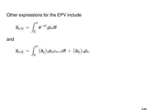
Other expressions for the EPV include

ax :n| =

∫ n

0e−δt tpxdt

and

ax :n| =

∫ n

0

(at |)

tpxµx+tdt +(an|)

npx .

5-22

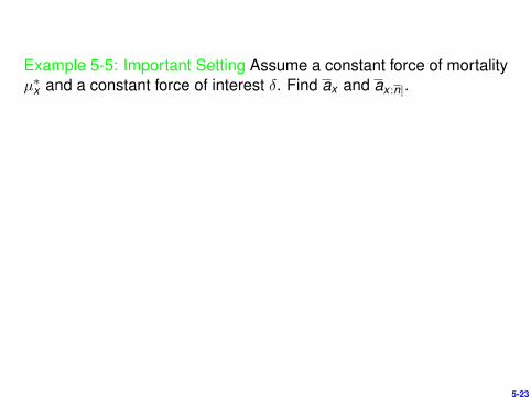
Example 5-5: Important Setting Assume a constant force of mortalityµ∗x and a constant force of interest δ. Find ax and ax :n|.

5-23

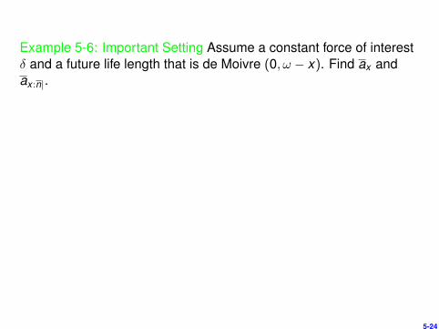
Example 5-6: Important Setting Assume a constant force of interestδ and a future life length that is de Moivre (0, ω − x). Find ax andax :n|.

5-24

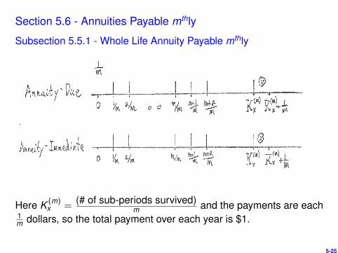
Section 5.6 - Annuities Payable mthly

Subsection 5.5.1 - Whole Life Annuity Payable mthly

Here K (m)x =

(# of sub-periods survived)m and the payments are each

1m dollars, so the total payment over each year is $1.

5-25

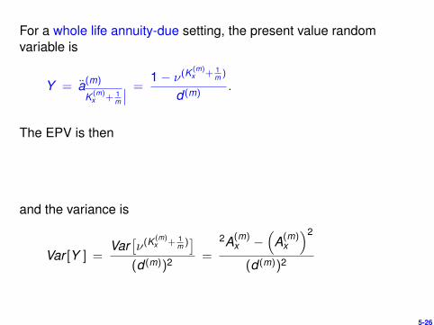
For a whole life annuity-due setting, the present value randomvariable is

Y = a(m)

K (m)x + 1

m

∣∣ =1− ν(K

(m)x + 1

m )

d (m).

The EPV is then

and the variance is

Var [Y ] =Var

[ν(K

(m)x + 1

m )]

(d (m))2 =

2A(m)x −

(A(m)

x

)2

(d (m))2

5-26

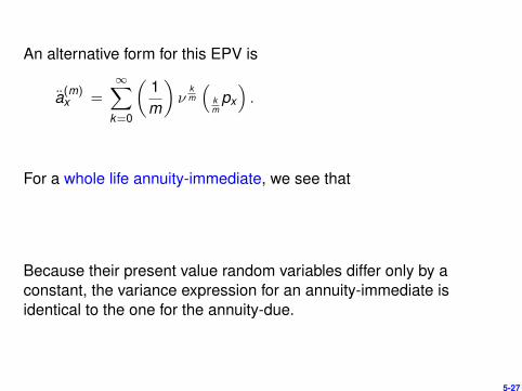
An alternative form for this EPV is

a(m)x =

∞∑k=0

(1m

)ν

km

(km

px

).

For a whole life annuity-immediate, we see that

Because their present value random variables differ only by aconstant, the variance expression for an annuity-immediate isidentical to the one for the annuity-due.

5-27

Subsection 5.6.2 - Term Life Annuity Payable mthly

When payments cease after n years, the present value randomvariable of the annuity-due is:

Y = a(m)

min(K (m)x + 1

m ,n)∣∣ =

1− νmin(K (m)x + 1

m ,n)

d (m).

So its EPV is:

and its variance is

Var [Y ] =Var

[νmin(K (m)

x + 1m ,n)]

(d (m))2 =

2A(m)x :n| −

(A(m)

x :n|

)2

(d (m))2

where A(m)x :n| denotes an endowment EPV.

5-28

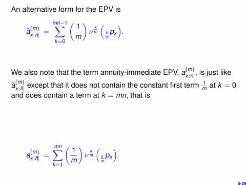
An alternative form for the EPV is

a(m)x :n| =

mn−1∑k=0

(1m

)ν

km

(km

px

).

We also note that the term annuity-immediate EPV, a(m)x :n|, is just like

a(m)x :n| except that it does not contain the constant first term 1

m at k = 0and does contain a term at k = mn, that is

a(m)x :n| =

mn∑k=1

(1m

)ν

km

(km

px

).

5-29

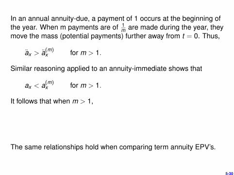
In an annual annuity-due, a payment of 1 occurs at the beginning ofthe year. When m payments are of 1

m are made during the year, theymove the mass (potential payments) further away from t = 0. Thus,

ax > a(m)x for m > 1.

Similar reasoning applied to an annuity-immediate shows that

ax < a(m)x for m > 1.

It follows that when m > 1,

The same relationships hold when comparing term annuity EPV’s.

5-30

Example 5-7: Mortality follows de Moivre (0,80) for someone age x.If δ = .05, find ax :20|.

5-31

Example 5-8: If Y is the present value R.V. for someone age x, findE [Y ] when

Y = an| when 0 ≤ Tx ≤ n and Y = aTx | otherwise.

5-32

Example 5-9: You are give that µ = .01 and that δ = .04 when0 ≤ t ≤ 5 and δ = .03 when t > 5. Find ax :10|.

5-33

Example 5-10: Given δ = .05 and µt = .05 for 0 ≤ t ≤ 50 andµt = .10 for t > 50. Find the EPV of a 50 year temporary lifecontinuous payment annuity with 1 smeared over each year forinsured age 30, ceasing immediately at death.

5-34

Example 5-11: A 30 year old will receive $5,000 annually beginningone year from today for as long as this person lives. When px = k forall x , the actuarial PV of the annuity is $22,500, with i = .10. Find k .

5-35

Example 5-12: Given Ax = .28, Ax+20 = .40, A 1x :20| = .25 and

i = .05, find ax :20| .

5-36

Section 5.8 - Deferred Life Annuities

A deferred life annuity does not begin payments until u years havepassed and then continues to make annual payments of 1 as long asthe annuitant is alive at the time of payment.

Here Kx is the number of whole years survived by the annuitant, i.e.Kx = bTxc. Also the distinction between an annuity-due and anannuity-immediate is moot in this setting. We could use either, butchoose to use annuity-due.

5-37

Let

Yx = ( 1 paid at the beginning of each year through Kx) and

Yx :u| = ( 1 paid at the beginning of each year through Kx ,

with a maximum of u payments).

The present value random variable for the deferred life annuity wouldthen be

u|Yx = Yx − Yx :u|.

It follows that the EPV is

5-38

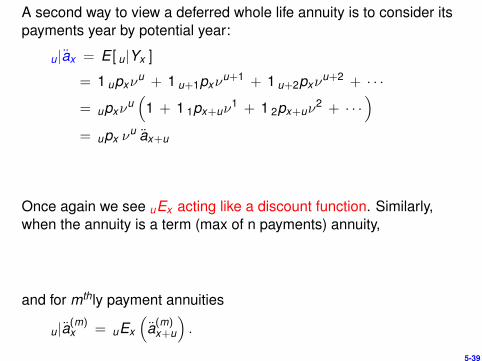
A second way to view a deferred whole life annuity is to consider itspayments year by potential year:

u|ax = E [ u|Yx ]

= 1 upxνu + 1 u+1pxν

u+1 + 1 u+2pxνu+2 + · · ·

= upxνu(

1 + 1 1px+uν1 + 1 2px+uν

2 + · · ·)

= upx νu ax+u

Once again we see uEx acting like a discount function. Similarly,when the annuity is a term (max of n payments) annuity,

and for mthly payment annuities

u|a(m)x = uEx

(a(m)

x+u

).

5-39

Example 5-13: A continuous deferred annuity pays at a rate of(1.04)t at time t starting 5 years from now. You are given δ = .07and µt = .01 when t < 5 and µt = .02 when t ≥ 5. Find the actuarialpresent value of this annuity.

5-40

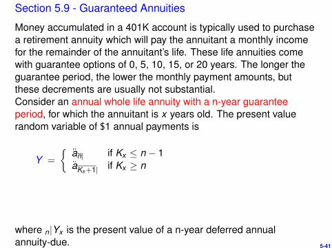
Section 5.9 - Guaranteed Annuities

Money accumulated in a 401K account is typically used to purchasea retirement annuity which will pay the annuitant a monthly incomefor the remainder of the annuitant’s life. These life annuities comewith guarantee options of 0, 5, 10, 15, or 20 years. The longer theguarantee period, the lower the monthly payment amounts, butthese decrements are usually not substantial.Consider an annual whole life annuity with a n-year guaranteeperiod, for which the annuitant is x years old. The present valuerandom variable of $1 annual payments is

Y =

{an| if Kx ≤ n − 1aKx+1| if Kx ≥ n

where n|Yx is the present value of a n-year deferred annualannuity-due. 5-41

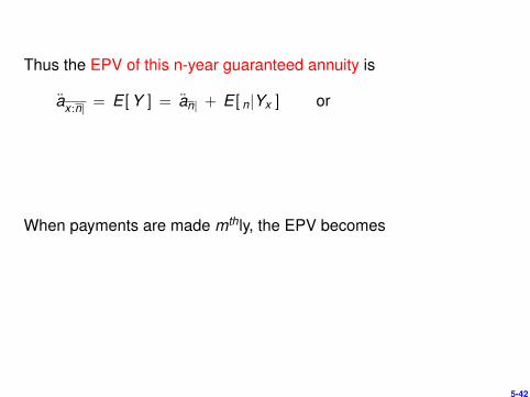
Thus the EPV of this n-year guaranteed annuity is

ax :n| = E [Y ] = an| + E [ n|Yx ] or

When payments are made mthly, the EPV becomes

5-42

Example 5-14: Given Ax = .3, Ax :20| = .4, i = .05 and 20px = .7, finda

x :20|.

5-43

Example 5-15: An annuity pays 1 at the beginning of each year for(35) and pays until age 65. Payments are certain for the first 15years. Calculate the EPV given: a15| = 11.94, a30| = 19.6,a35:15| = 11.62, a35:30| = 18.13, a35 = 21.02, a50 = 15.66 anda65 = 9.65 .

5-44

Section 5.10 - Life Annuities With Increasing Payments

Subsection 5.10.1 - Arithmetically Increasing Annuities

Consider the arithmetically increasing sequence of life contingentpayments pictured above. The EPV of these payments is

5-45

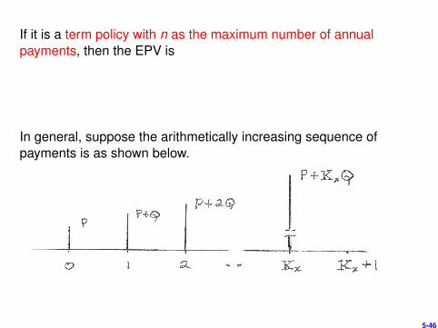
If it is a term policy with n as the maximum number of annualpayments, then the EPV is

In general, suppose the arithmetically increasing sequence ofpayments is as shown below.

5-46

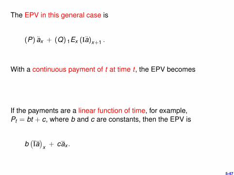
The EPV in this general case is

(P) ax + (Q) 1Ex (Ia)x+1 .

With a continuous payment of t at time t , the EPV becomes

If the payments are a linear function of time, for example,Pt = bt + c, where b and c are constants, then the EPV is

b(Ia)

x + cax .

5-47

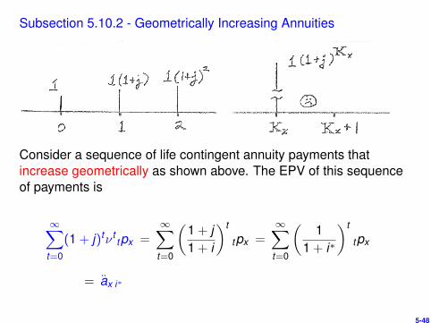
Subsection 5.10.2 - Geometrically Increasing Annuities

Consider a sequence of life contingent annuity payments thatincrease geometrically as shown above. The EPV of this sequenceof payments is

∞∑t=0

(1 + j)tν ttpx =

∞∑t=0

(1 + j1 + i

)t

tpx =∞∑

t=0

(1

1 + i∗

)t

tpx

= ax i∗

5-48

Here i∗ is the interest rate that satisfies

Example 5-16: An injured worker is to receive annual annuitypayments beginning today with a payment of $100K. Subsequentpayments increase by 2% each year. If i = .05 and tpx = (.7)t for0 ≤ t ≤ 5 and tpx = 0 for t > 5, find the EPV.

5-49

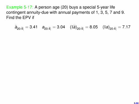
Example 5-17: A person age (20) buys a special 5-year lifecontingent annuity-due with annual payments of 1, 3, 5, 7 and 9.Find the EPV if

a20:4| = 3.41 a20:4| = 3.04 (Ia)20:4| = 8.05 (Ia)20:4| = 7.17

5-50

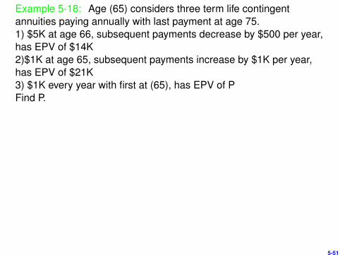
Example 5-18: Age (65) considers three term life contingentannuities paying annually with last payment at age 75.1) $5K at age 66, subsequent payments decrease by $500 per year,has EPV of $14K2)$1K at age 65, subsequent payments increase by $1K per year,has EPV of $21K3) $1K every year with first at (65), has EPV of PFind P.

5-51

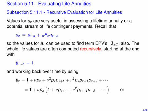
Section 5.11 - Evaluating Life Annuities

Subsection 5.11.1 - Recursive Evaluation for Life Annuities

Values for ax are very useful in assessing a lifetime annuity or apotential stream of life contingent payments. Recall that

ax = ax :n + nEx ax+n

so the values for ax can be used to find term EPV’s , ax :n, also. Thewhole life values are often computed recursively, starting at the endwith

aω−1 = 1,

and working back over time by using

ax = 1 + νpx + ν2pxpx+1 + ν3pxpx+1px+2 + · · ·

= 1 + νpx

(1 + νpx+1 + ν2px+1px+2 + · · ·

)or

5-52

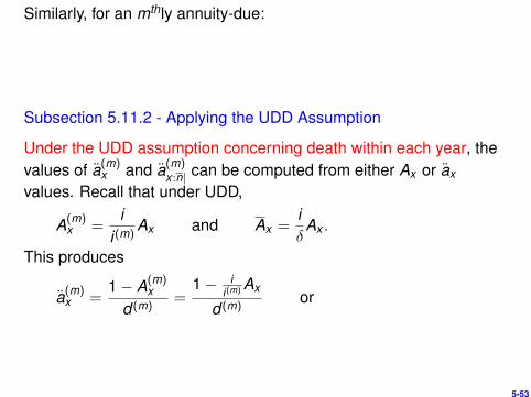
Similarly, for an mthly annuity-due:

Subsection 5.11.2 - Applying the UDD Assumption

Under the UDD assumption concerning death within each year, thevalues of a(m)

x and a(m)x :n| can be computed from either Ax or ax

values. Recall that under UDD,

A(m)x =

ii(m)

Ax and Ax =iδ

Ax .

This produces

a(m)x =

1− A(m)x

d (m)=

1− ii(m) Ax

d (m)or

5-53

Now use the fact that ax = 1−Axd and write

a(m)x =

i(m) − i(1− dax)

i(m)d (m)=

(id

i(m)d (m)

)ax −

(i − i(m)

i(m)d (m)

)or

As m→∞, we get

because limm→∞ i(m) = δ = limm→∞ d (m) .

5-54

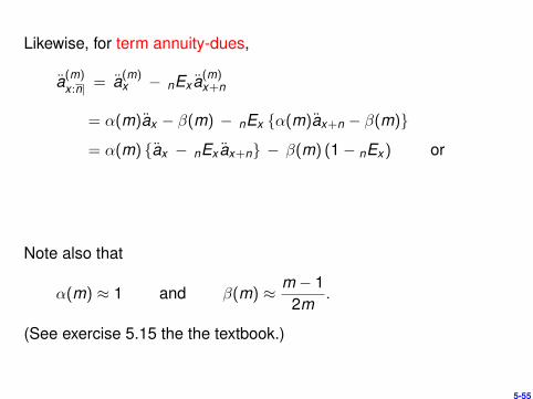
Likewise, for term annuity-dues,

a(m)x :n| = a(m)

x − nEx a(m)x+n

= α(m)ax − β(m) − nEx {α(m)ax+n − β(m)}

= α(m) {ax − nEx ax+n} − β(m) (1− nEx) or

Note also that

α(m) ≈ 1 and β(m) ≈ m − 12m

.

(See exercise 5.15 the the textbook.)

5-55

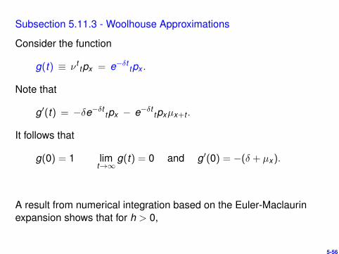
Subsection 5.11.3 - Woolhouse Approximations

Consider the function

g(t) ≡ ν ttpx = e−δt tpx .

Note that

g′(t) = −δe−δt tpx − e−δt tpxµx+t .

It follows that

g(0) = 1 limt→∞

g(t) = 0 and g′(0) = −(δ + µx).

A result from numerical integration based on the Euler-Maclaurinexpansion shows that for h > 0,

5-56

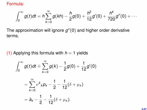
Formula:∫ ∞0

g(t)dt = h∞∑

k=0

g(kh)− h2

g(0) +h2

12g′(0) +

h4

720g′′(0) + · · ·

The approximation will ignore g′′(0) and higher order derivativeterms.

(1) Applying this formula with h = 1 yields∫ ∞0

g(t)dt .=∞∑

k=0

g(k)− 12

g(0) +1

12g′(0)

=∞∑

k=0

νkkpx −

12− 1

12(δ + µx)

= ax −12− 1

12(δ + µx).

5-57

(2) Applying this formula with h = 1m yields∫ ∞

0g(t)dt .

=1m

∞∑k=0

g(km)− 1

2mg(0) +

112m2 g′(0)

=1m

∞∑k=0

νkm k

mpx −

12m− 1

12m2 (δ + µx)

= a(m)x − 1

2m− 1

12m2 (δ + µx).

5-58

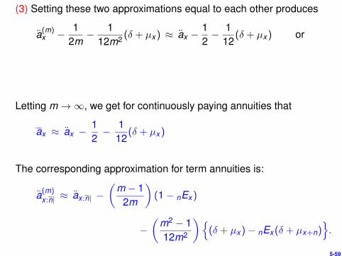
(3) Setting these two approximations equal to each other produces

a(m)x − 1

2m− 1

12m2 (δ + µx) ≈ ax −12− 1

12(δ + µx) or

Letting m→∞, we get for continuously paying annuities that

ax ≈ ax −12− 1

12(δ + µx)

The corresponding approximation for term annuities is:

a(m)x :n| ≈ ax :n| −

(m − 1

2m

)(1− nEx)

−(

m2 − 112m2

){(δ + µx)− nEx(δ + µx+n)

}.

5-59

The Woolhouse approximations above require the use of µx . Withlife table data, we can approximate µx as follows:

2px−1 = pxpx−1 = e−∫ x+1

x−1 µsds ≈ e−2µx .

This motivates

where px =lx+1lx .

5-60

Section 5.13 - Select Lives in Life Annuities

Selection via underwriting alters the survival probabilities which intern alter the present values of payment streams. For example,

ax =∞∑

k=0

νkkp[x ]

5-61