chapter 5: the schumpeterian model - brown university · chapter 5: the schumpeterian model...

Chapter 5: The Schumpeterian Model∗

Philippe Aghion Ufuk Akcigit Peter Howitt

May 21, 2014

5.1 Introduction

This chapter develops an alternative model of endogenous growth, in which growth is generated

by a random sequence of quality-improving (or “vertical”) innovations. The model grew out of

modern industrial organization theory1, which portrays innovation as an important dimension of

industrial competition. This model is Schumpeterian in that: (i) it is about growth generated by

innovations; (ii) innovations result from entrepreneurial investments that are themselves motivated

by the prospects of monopoly rents; and (iii) new innovations replace old technologies: in other

words, growth involves creative destruction.

Over the past 25 years,2 Schumpeterian growth theory has developed into an integrated frame-

work for understanding not only the macroeconomic structure of growth but also the many mi-

croeconomic issues regarding incentives, policies and organizations that interact with growth: who

gains and who loses from innovations, and what the net rents from innovation are; these ultimately

depend on characteristics such as property right protection, competition and openness, education,

democracy and so forth and to a different extent in countries or sectors at different stages of de-

velopment. Moreover, the recent years have witnessed a new generation of Schumpeterian growth

∗Very Preliminary. Please do not circulate. In class use only. Please report all typos/mistakes to [email protected].

1See Tirole (1988).2The approach was initiated in the fall of 1987 at MIT, where Philippe Aghion was a first-year assistant professor

and Peter Howitt a visiting professor on sabbatical from the University of Western Ontario. During that year theywrote their "model of growth through creative destruction" (see Section 5.3 below); which was published as Aghionand Howitt (1992). Parallel attempts at developing Schumpeterian growth models include Segerstrom, Anant andDinopoulos (1990) and Corriveau (1991).

1

New Growth Economics Chapter 5 Aghion et al.

models focusing on firm dynamics and reallocation of resources among incumbents and new en-

trants.3 These models are easily estimable using micro firm-level datasets, which also bring the rich

set of tools from other empirical fields into macroeconomics and endogenous growth. Subsequent

chapters will describe each of these applications in great detail.

This model of growth with vertical innovations has the natural property that new inventions

make old technologies or products obsolete. This obsolescence (or “creative destruction”) feature

in turn has both positive and normative consequences. On the positive side it implies a negative

relationship between current and future research, which results in the existence of a unique steady-

state (or balanced growth) equilibrium. On the normative side, although current innovations have

positive externalities for future research and development, they also exert a negative externality on

incumbent producers. This business-stealing effect in turn introduces the possibility that growth

be excessive under laissez-faire, a possibility that did not arise in the endogenous growth models

surveyed in the previous chapter.

In this chapter, we describe the basics of the Schumpeterian framework. In particular, Section

5.2 presents a simple discrete time version of the Schumpeterian growth model. Section 5.3 then

presents a continuous time version of the one-sector Schumpeterian model. Section 5.4 then extends

the continuous time model to multiple sectors.

5.2 A toy (myopic-agents) version of the Schumpeterian model

In this section we develop a simple version of the Schumpeterian growth model with discrete

time and where individuals and firms live for one period. The basic model abstracts from capital

accumulation completely.4 There is a unique “final” good in this economy, Yt, which is used for

consumption Ct, intermediate good production Xt, and R&D Rt. Therefore the resources constraint

of this economy is simply

Yt = Ct +Xt +Rt.

3See Klette and Kortum (2004), Lentz and Mortensen (2008), Akcigit and Kerr (2010), and Acemoglu, Akcigit,Bloom and Kerr (2013)

4The implications of introducing human and physical capital accumulation are explored in Chapter XXX.

Very preliminary notes, Please do not circulate! 2


5.2.1 The production technology

There is a sequence of discrete time periods t = 1, 2, ... Each period there is a fixed number L of

individuals, each of whom lives for just that period and is endowed with one unit of labor services

which she supplies inelastically. Her utility depends only on her consumption and she is risk-neutral,

so she has the single objective of maximizing expected consumption.

People consume only one good, called the “final”good, which is produced by perfectly competi-

tive firms using two inputs - labor and a single intermediate product - according to the Cobb-Douglas

production function:

Yt = (AtLt)1−α yαt (5.1)

where Yt is output of the final good in period t, At is a parameter that reflects the productivity

of the intermediate input that period and yt is the amount of intermediate product used. The

coeffi cient α lies between zero and one. The economy’s entire labor supply L is used in final-good

production. As in the neoclassical model, we refer to the product AtL as the economy’s effective

labor supply. We normalize the price of the final good to unity without loss of any generality.

The intermediate product is produced by a monopolist each period, using the final good as an

input, one for one. Let us denote the amount of final good used for intermediate-good production

by Xt. Then the production function is simply

yt = Xt. (5.2)

That is, for each unit of intermediate product, the monopolist must use one unit of final good as

input.

5.2.2 Innovation

Growth results from innovations that raise the productivity parameter At by improving the quality

of the intermediate product. Each period there is one person (the “entrepreneur”) who has an

opportunity to attempt an innovation. If she succeeds, the innovation will create a new version

of the intermediate product, which is more productive than previous versions. Let us denote last



period’s productivity as At−1. Specifically, the productivity of the intermediate good in use will go

from last period’s value At−1 up to At = γAt−1, where γ > 1. On the other hand, if she fails then

there will be no innovation at t and, in this case, another randomly chosen monopolist will produce

the intermediate good with the old productivity that was used in t− 1, so At = At−1. Hence

At =

γAt−1 if entrepreneur is successful,

At−1 if entrepreneur fails.(5.3)

In order to innovate, the entrepreneur must conduct research, a costly activity that uses the

final good as its only input. As indicated above, research is uncertain, for it may fail to generate any

innovation. But the more the entrepreneur spends on research the more likely she is to innovate.

Specifically, we assume to innovate from At−1 up to At = γAt−1 with probability zt, one must

spend the amount

Rt = c(zt)At−1 (5.4)

final good on research.

For simplicity, assume a quadratic R&D cost:

c(zt) = δz2t /2, (5.5)

where δ is a parameter which inversely measures the productivity of the research sector.

Timing of events Now we can summarize the timing of events in this model:

• step 0 Period t begins with the initial productivity At−1 which is inherited from the previous

period (cohort),

• step 1 a randomly chosen entrepreneur invests in R&D by chosing (zt, Rt),

• step 2 innovation (success/failure) is realized, and productivity evolves according to (5.3) ,

• step 3 production of the intermediate good (yt) takes place,

• step 4 production of the final good (Yt) takes place,

• step 5 consumption (Ct) takes place, and period t ends.



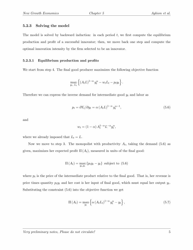
5.2.3 Solving the model

The model is solved by backward induction: in each period t, we first compute the equilibrium

production and profit of a successful innovator; then, we move back one step and compute the

optimal innovation intensity by the firm selected to be an innovator.

5.2.3.1 Equilibrium production and profits

We start from step 4. The final good producer maximizes the following objective function

maxyt, Lt

{(AtL)1−α yαt − wtLt − ptyt

}.

Therefore we can express the inverse demand for intermediate good yt and labor as

pt = ∂Yt/∂yt = α (AtL)1−α yα−1t , (5.6)

and

wt = (1− α)A1−αt L−αyαt ,

where we already imposed that Lt = L.

Now we move to step 3. The monopolist with productivity At, taking the demand (5.6) as

given, maximizes her expected profit Π (At), measured in units of the final good:

Π (At) = maxyt,pt{ptyt − yt} subject to (5.6)

where pt is the price of the intermediate product relative to the final good. That is, her revenue is

price times quantity ptyt and her cost is her input of final good, which must equal her output yt.

Substituting the constraint (5.6) into the objective function we get

Π (At) = maxyt

{α (AtLt)

1−α yαt − yt}, (5.7)



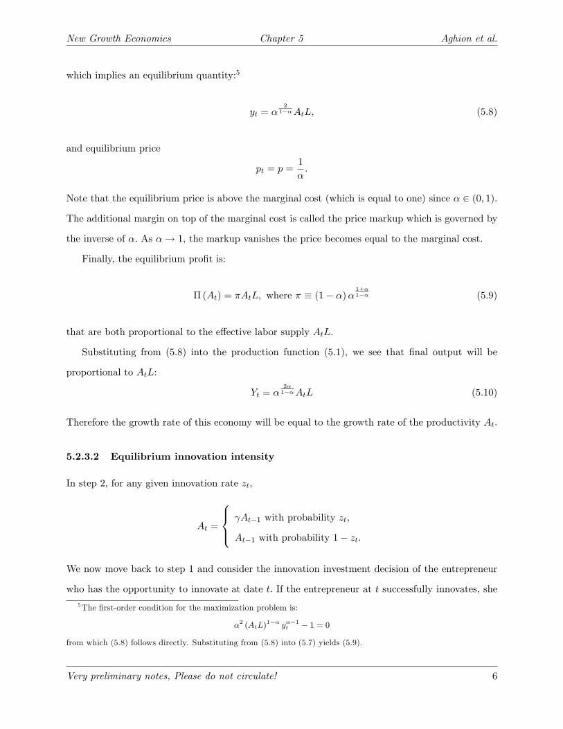
which implies an equilibrium quantity:5

yt = α2

1−αAtL, (5.8)

and equilibrium price

pt = p =1

α.

Note that the equilibrium price is above the marginal cost (which is equal to one) since α ∈ (0, 1).

The additional margin on top of the marginal cost is called the price markup which is governed by

the inverse of α. As α→ 1, the markup vanishes the price becomes equal to the marginal cost.

Finally, the equilibrium profit is:

Π (At) = πAtL, where π ≡ (1− α)α1+α1−α (5.9)

that are both proportional to the effective labor supply AtL.

Substituting from (5.8) into the production function (5.1), we see that final output will be

proportional to AtL:

Yt = α2α1−αAtL (5.10)

Therefore the growth rate of this economy will be equal to the growth rate of the productivity At.

5.2.3.2 Equilibrium innovation intensity

In step 2, for any given innovation rate zt,

At =

γAt−1 with probability zt,

At−1 with probability 1− zt.

We now move back to step 1 and consider the innovation investment decision of the entrepreneur

who has the opportunity to innovate at date t. If the entrepreneur at t successfully innovates, she

5The first-order condition for the maximization problem is:

α2 (AtL)1−α yα−1t − 1 = 0

from which (5.8) follows directly. Substituting from (5.8) into (5.7) yields (5.9).



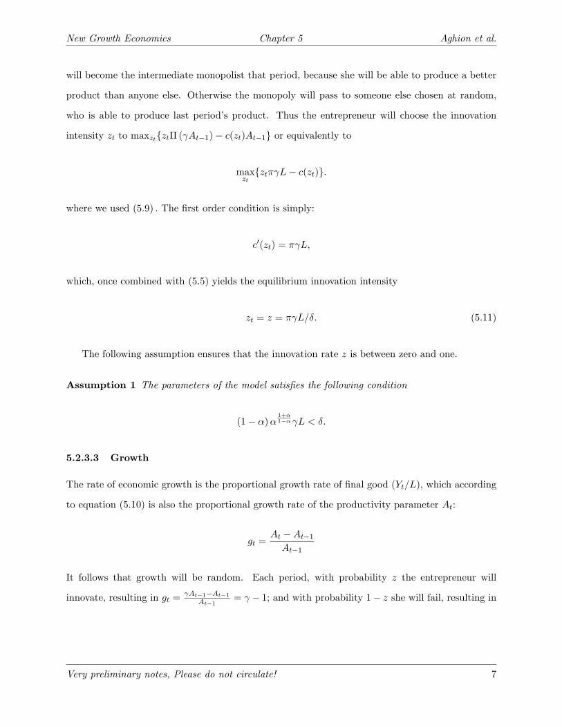
will become the intermediate monopolist that period, because she will be able to produce a better

product than anyone else. Otherwise the monopoly will pass to someone else chosen at random,

who is able to produce last period’s product. Thus the entrepreneur will choose the innovation

intensity zt to maxzt{ztΠ (γAt−1)− c(zt)At−1} or equivalently to

maxzt{ztπγL− c(zt)}.

where we used (5.9) . The first order condition is simply:

c′(zt) = πγL,

which, once combined with (5.5) yields the equilibrium innovation intensity

zt = z = πγL/δ. (5.11)

The following assumption ensures that the innovation rate z is between zero and one.

Assumption 1 The parameters of the model satisfies the following condition

(1− α)α1+α1−αγL < δ.

5.2.3.3 Growth

The rate of economic growth is the proportional growth rate of final good (Yt/L), which according

to equation (5.10) is also the proportional growth rate of the productivity parameter At:

gt =At −At−1At−1

It follows that growth will be random. Each period, with probability z the entrepreneur will

innovate, resulting in gt = γAt−1−At−1At−1

= γ − 1; and with probability 1− z she will fail, resulting in



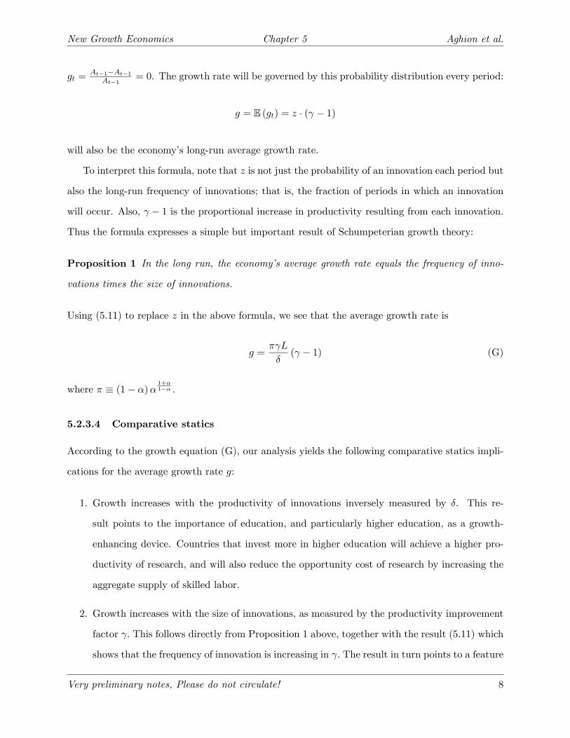
gt = At−1−At−1At−1

= 0. The growth rate will be governed by this probability distribution every period:

g = E (gt) = z · (γ − 1)

will also be the economy’s long-run average growth rate.

To interpret this formula, note that z is not just the probability of an innovation each period but

also the long-run frequency of innovations; that is, the fraction of periods in which an innovation

will occur. Also, γ − 1 is the proportional increase in productivity resulting from each innovation.

Thus the formula expresses a simple but important result of Schumpeterian growth theory:

Proposition 1 In the long run, the economy’s average growth rate equals the frequency of inno-

vations times the size of innovations.

Using (5.11) to replace z in the above formula, we see that the average growth rate is

g =πγL

δ(γ − 1) (G)

where π ≡ (1− α)α1+α1−α .

5.2.3.4 Comparative statics

According to the growth equation (G), our analysis yields the following comparative statics impli-

cations for the average growth rate g:

1. Growth increases with the productivity of innovations inversely measured by δ. This re-

sult points to the importance of education, and particularly higher education, as a growth-

enhancing device. Countries that invest more in higher education will achieve a higher pro-

ductivity of research, and will also reduce the opportunity cost of research by increasing the

aggregate supply of skilled labor.

2. Growth increases with the size of innovations, as measured by the productivity improvement

factor γ. This follows directly from Proposition 1 above, together with the result (5.11) which

shows that the frequency of innovation is increasing in γ. The result in turn points to a feature



that will become important when we discuss cross-country convergence. A country that lags

behind the world technology frontier has what Gerschenkron (1962) called an advantage of

backwardness. That is, the further it lags behind the frontier, the bigger the productivity

improvement it will get if it can implement the frontier technology when it innovates, and

hence the faster it can grow.

3. An increase in the size of population should also bring about an increase in growth by raising

the supply of labor L. This “scale effect”is also present in the product variety model, and has

been challenged in the literature. In Appendix A.4.2 below we will see how this questionable

comparative statics result can be eliminated by considering a model with both horizontal and

vertical innovations.

5.2.3.5 Welfare Analysis

In this simplified framework, we can now ask the following question: What is the socially optimal

level of production and R&D investment in this economy? To answer this question, we first need

to take a stand on the objective function of the social planner. To be inline with this section, we

consider a myopic social planner that maximizes the period-by-period utility which is equivalent to

maximizing the per-period consumption.

We again follow a backward induction argument. Recall that the level of consumption from the

resource constraint is simply

Ct = Yt −Xt −Rt.

In step 4, therefore, the social planner maximizes consumption subject to final good and interme-

diate good production technologies (5.1) and (5.2) . Note that in step 4, the R&D investment is

already made, hence Rt is taken as constant at this stage. Let us denote the household’s maximum

consumption, for any given producitivity At and the sunk R&D investment Rt, by C (At, Rt) . Then

the planner’s maximization can be rewritten as

C (At, Rt) ≡ maxyt

{(AtL)1−α yαt − yt −Rt

}.



From this maximization, the socially optimal level of intermediate good production is

yspt = AtLα1

1−α (5.12)

and the resulting maximum consumption is

C (At, Rt) ≡ AtLαα

1−α (1− α)−Rt. (5.13)

Now we can combine (5.12) with (5.1) to express the socially optimal GDP as

Y spt = AtLα

α1−α . (5.14)

Remark 2 We can already see the first distortion in this economy. The comparison of (5.12) to

(5.8) and (5.14) to (5.10) indicate

yspt > yt and Yspt > Yt

which implies that the decentralized economy underproduces output due to “monopoly distortions”.

Now we go one step back in social planner’s problem and specify the maximization problem for

the optimal innovation decision as: Cspt ≡ maxzt{ztC (γAt−1, Rt)+(1− zt) C (At−1, Rt)} subject to

the R&D technology (5.4) . Substituting the constraint into the objective function we can express

the planner’s innovation problem as

Cspt ≡ maxzt{ztγAt−1Lα

α1−α (1− α) + (1− zt)At−1Lα

α1−α (1− α)− δz2t

2At−1}. (5.15)

Note here the the social planner compares the consumption level upon a successful innovation

to consumption in the case of a failure, which implies that the innovation size plays a crucial

role for the social planner. However, in the decentralized economy, the entrepreneur cares only

about the success since in the case of a failure, the market is served by another firm. Therefore

the entrepreneur does not internalize the size of the innovation γ as the social planner does and

therefore creates an innovation externality.



Now we can find the socially optimal innovation rate by taking the first-order condition of (5.15)

zspt = (γ − 1)Lα

α1−α (1− α)

δ(5.16)

Remark 3 Comparing (5.16) to (5.11), we find underinvestment in R&D (zt < zspt ) if and only if

α1

1−α <γ − 1

γ.

This result is very intuitive. In this economy, there are two types ineffi ciencies: (i) Monopoly

distortion, and (ii) innovation externality.

The former is governed by the parameter α, which determines the equilibrium markups. The

latter is governed by γ as described above. Therefore, if the innovation externalities are above a

threshold (high γ), then the economy features underinvestment in R&D and vice versa.

5.2.4 Industrial Policy

In this section, we will consider the role of industrial policy in the simplified Schumpeterian frame-

work. As Remarks 2 and 3 have shown, the decentralized economy is not effi cient. This implies

that the policymaker can improve the welfare in this economy by using standard policy tools such

as production subsidy or R&D subsidy. This is what we are going to study next.

Assume that the government subsidizes production and R&D at the rates τP and τR, respec-

tively. Now we will find the optimal (welfare maximizing) rates of τP and τR. For simplicity, we

assume that the government finances these subsidies through lump-sum taxes on the household.

Production subsidy Let us rewrite equation (5.7) , the production decision of the monopo-

list, this time with the production subsidy:

Πτ (At) = maxyt

{α (AtL)1−α yαt −

(1− τP

)yt

}.

The resulting output is

yτt =

[α2

1− τP

] 11−α

AtL. (5.17)



Now we can find the optimal subsidy rate by equating (5.17) to (5.12)

τP = 1− α.

Our first finding is that the production subsidy is decreasing in α. This should not be surprising since

τP here corrects for monopoly distortions and recall that the monopoly markups are decreasing in

α. Hence a higher α implies a lower distortion and hence a lower subsidy rate τP .

Under the optimal production subsidy, the equilibrium profit is

Πτ (At) = AtLα1

1−α (1− α)

R&D subsidy Now assume that the government is already imposing the optimal production

subsidy τP = 1 − α and also subsidizes R&D at the rate τR. Then the innovation decision of the

entrepreneur is

maxzt{ztγAt−1Lα

11−α (1− α)−

(1− τR

) δz2t2At−1}.

Then the optimal choice of the entrepreneur is

zτt =γLα

11−α (1− α)

(1− τR) δ

Now equating this innovation rate to the socially optimal rate in (5.16)

τR = 1− αγ

(γ − 1)

Note that∂τR

∂γ> 0 and

∂τR

∂α< 0.

This implies the the optimal R&D subsidy rate is increasing in the size of the innovation γ. This

is intuitive because as we saw in Remark 3, one of the main ineffi ciencies in R&D spending is the

uninternalized contribution of each innovation, which is measured by γ.



5.2.5 Multisector extension

In this section we allow for multiple innovating sectors in the economy. Suppose there is not one

intermediate product but a continuum, indexed on the interval [0, 1] . The final-good production

function is now:

Yt = L1−α∫ 1

0A1−αit yαitdi, (5.18)

where each yit is the flow of intermediate product i used at t, and the productivity parameter Ait

reflects the quality of that product. In any period the productivity parameters will vary across

intermediate products because of the randomness of the innovation process.

According to (5.18), the final output produced by each intermediate product is determined by

the production function:

Yit = (AitL)1−α yαit (5.19)

which is identical to the production function (5.1) of the one-sector model. The final good producer’s

maximization problem is

maxLt,{yit}i∈[0,1]

{L1−αt

∫ 1

0A1−αit yαitdi− wtLt −

∫ 1

0pityitdi

}.

Each intermediate product has its own monopoly, and its price equals its marginal product in

the final sector, which according to (5.19) is

pit = ∂Yit/∂yit = α (AitL)1−α yα−1it . (5.20)

Similarly, the profit maximizing labor choice is

wt = ∂Yit/∂Lt

= (1− α)L−α∫ 1

0A1−αit yαitdi

where the second line uses the labor market clearing, Lt = L.

Now, the monopolist in sector i takes the demand for its product (5.20) as given and chooses



the quantity yit that maximizes her profit:

Π (Ait) = maxyit{pityit − yit} = max

yit

{α (AitL)1−α yαit − yit

}, (5.21)

which implies an equilibrium quantity:6

yit = α2

1−αAitL (5.22)

and an equilibrium profit:

Π (Ait) = πAitL. (5.23)

where the parameter π is the same as in the analogous equation (5.9) of the one-sector model.

The aggregate behavior of the economy depends on the aggregate (which also corresponds to

average in this case) productivity index:

At =

∫ 1

0Aitdi

which is just the unweighted numerical average of all the individual productivities. In particular,

final output and GDP in this multisector economy are determined by exactly the same equations

as in the one-sector economy of the previous section, but with At now being this average, instead

of being the productivity of the economy’s only intermediate product.

More specifically, using (5.22) to substitute for each yit in the production function (5.18) yields

the same formula as before for final output:

Yt = α2α1−αAtL (5.24)

6The first-order condition for the maximization problem is:

α2 (AitL)1−α yα−1it − 1 = 0

from which (5.22) follows directly. Substituting from (5.22) into (5.21) yields (5.23).



5.2.5.1 Innovation and research arbitrage

Innovation in each sector takes place exactly as in the one-sector model. Specifically, there is a

single entrepreneur in each sector who spends final output in research and to innovate from Ait−1

up to Ait = γAit−1 with probability zt. In order to achieve this, she needs to spend the amount of

final good

Rit = c(zt)Ait−1

in research.

The entrepreneur chooses the innovation intensity zit that maximizes her net expected benefit:

maxzt∈[0,1]

{ztΠ (γAit−1)− c(zt)Ait−1}

which yields

zit ≡ z = πγL/δ. (5.25)

This exactly the same as the research effort in the one-sector model. One important feature of

this model is that the probability of innovation z is the same in all sectors, no matter what the

starting level of productivity Ai,t−1. This might seem surprising, because the reward Π (γAit−1) =

πγAi,t−1L to a successful innovation is higher in more advanced sectors. But this advantage is just

offset by the fact that the cost of innovating at any given rate is also correspondingly higher because

what matters is research expenditure relative to the current productivity level Ai,t−1. As we will

see, this feature allows a simple characterization of the aggregate growth rate in the economy.

5.2.5.2 Growth

Since per-capita GDP is again proportional to the aggregate productivity At (see equation (5.24)),

therefore the economy’s growth rate is again the proportional growth rate of At:

gt =At −At−1At−1

(5.26)



In this case, however, the aggregate growth rate is no longer random, because bad luck in some

sectors will be offset by good luck in others.

In each sector i we have:

Ait =

γAi,t−1 with probability z

Ai,t−1 with probability 1− z

(5.27)

Recall that the average productivity is At =∫ 10 Aitdi. We can express next period’s average pro-

ductivity as

At =

∫ 1

0[zγAit−1 + (1− z)Ait−1] di =

∫ 1

0Ait−1di+ z (γ − 1)

∫ 1

0Ait−1di

= At−1 + z (γ − 1)At−1

It follows from this and (5.26) that the growth rate each period is equal to the constant

g = z · (γ − 1)

which is the same as the long-run average growth rate of the one-sector model. Substituting (5.25)

into this formula produces the same expression (G) as before, implying the same comparative static

results as before.

5.3 The Aghion-Howitt model

Creative destruction was somewhat mechanical in the above discrete-time model, in that by as-

sumption firms were assumed to live for only one period and thus to be replaced by newly born

entrepreneurs. In this section we allow incumbent firms to remain on the market as long as they

have not been replaced by a new innovator. The expected average lifetime of a firm will thus be

equal to the inverse of the aggregate rate of innovation. This rate of innovation will in turn be

determined by a research arbitrage equation which factors in the rate of creative destruction.



5.3.1 The setup

Time is continuous and the economy is populated by a continuous mass L of infinitely lived in-

dividuals with linear preferences, that discount the future at rate ρ.7 Each individual is endowed

with one unit of labor per unit of time, which she can allocate between production and research:

in equilibrium, individuals are indifferent between these two activities.

There is a final good, which is also the numeraire. The final good at time t is produced

competitively using an intermediate input, namely:

Yt = Atyαt

where α is between zero and one, yt is the amount of the intermediate good currently used in

the production of the final good, and At is the productivity -or quality- of the currently used

intermediate input.8

The intermediate good y is in turn produced one for one with labor: that is, one unit flow of

labor currently used in manufacturing the intermediate input produces one unit of intermediate

input of frontier quality. Thus yt denotes both the current production of the intermediate input

and the flow amount of labor currently employed in manufacturing the intermediate good.

Growth in this model results from innovations that improve the quality of the intermediate

input used in the production of the final good. More formally, if the previous state-of-the-art

intermediate good was of quality A, then a new innovation will introduce a new intermediate input

of quality γA, where γ > 1. This immediately implies that growth will involve creative destruction,

in the sense that Bertrand competition will allow the new innovator to drive the firm producing

the intermediate good of quality A out of the market, since at the same labor cost the innovator

produces a better good than that of the incumbent firm.9

7The linear preferences (or risk neutrality) assumption implies that the equilibrium interest rate will always beequal to the rate of time preference: rt = ρ (see Aghion and Howitt (2009), Chapter 2).

8 In what follows we will use the words "productivity" and "quality" interchangeably.9Thus, overall, growth in the Schumpeterian model involves both positive and negative externalities. The positive

externality is referred to by Aghion and Howitt (1992) as a "knowledge spillover effect": namely, any new innovationraises productivity A forever, i.e., the benchmark technology for any subsequent innovation; however, the current(private) innovator captures the rents from her innovation only during the time interval until the next innovationoccurs. This effect is also featured in Romer (1990), where it is referred to instead as "non-rivalry plus limitedexcludability." But in addition, in the Schumpeterian model, any new innovation has a negative externality as itdestroys the rents of the previous innovator: following the theoretical IO literature, Aghion and Howitt (1992)



The innovation technology is directly drawn from the theoretical IO and patent race literatures:

namely, if zt units of labor are currently used in R&D, then a new innovation arrives during the

current unit of time at the (memoryless) Poisson rate λzt.10 Henceforth we will drop the time

index t, when it causes no confusion.


5.3.2.1 The research arbitrage and labor market clearing equations

We shall concentrate our attention on balanced growth equilibria where the allocation of labor

between production (y) and R&D (z) remains constant over time. The growth process is described

by two basic equations.

The first is the labor market clearing equation:

L = y + z (L)

reflecting the fact that the total flow of labor supply during any unit of time is fully absorbed

between production and R&D activities (i.e., by the demand for manufacturing and R&D labor).

The second equation reflects individuals’indifference in equilibrium between engaging in R&D or

working in the intermediate good sector. We call it the research arbitrage equation. The remaining

part of the analysis consists of spelling out this research arbitrage equation.

More formally, let wk denote the current wage rate conditional on there having already been

k ∈ Z++ innovations from time 0 until current time t (since innovation is the only source of change

in this model, all other economic variables remain constant during the time interval between two

successive innovations). And let Vk+1 denote the net present value of becoming the next ((k + 1)

-th) innovator.

During a small time interval dt, between the k-th and (k + 1) -th innovations, an individual

faces the following choice. Either she employs her (flow) unit of labor for the current unit of time

refer to this as the "business-stealing effect" of innovation. The welfare analysis in that paper derives suffi cientconditions under which the intertemporal spillover effect dominates or is dominated by the business-stealing effect.The equilibrium growth rate under laissez-faire is correspondingly suboptimal or excessive compared to the sociallyoptimal growth rate.10More generally, if zt units of labor are invested in R&D during the time interval [t, t + dt], the probability of

innovation during this time interval is λztdt.



in manufacturing at the current wage, in which case she gets wtdt. Or she devotes her flow unit

of labor to R&D, in which case she will innovate during the current time period with probability

λdt and then get Vk+1, whereas she gets nothing if she does not innovate.11 The research arbitrage

equation is then simply expressed as:

wk = λVk+1. (R)

The value Vk+1 is in turn determined by a Bellman equation. We will use Bellman equations

repeatedly in this survey; thus, it is worth going slowly here. During a small time interval dt, a firm

collects πk+1dt profits. At the end of this interval, it is replaced by a new entrant with probability

λzdt through creative destruction; otherwise, it preserves the monopoly power and Vk+1. Hence

the value function is written as

Vk+1 = πk+1dt+ (1− rdt)

λzdt× 0+

(1− λzdt)× Vk+1

Dividing both sides by dt, then taking the limit as dt→ 0 and using the fact that the equilibrium

interest rate is equal to the time preference, the Bellman equation for Vk+1 can be rewritten as:

ρVk+1 = πk+1 − λzVk+1.

In other words, the annuity value of a new innovation (i.e., its flow value during a unit of time)

is equal to the current profit flow πk+1 minus the expected capital loss λzVk+1 due to creative

destruction, i.e., to the possible replacement by a subsequent innovator. If innovating gave the

innovator access to a permanent profit flow πk+1, then we know that the value of the corresponding

perpetuity would be πk+1/r.12 However, there is creative destruction at rate λz. As a result, we

11Note that we are implicitly assuming that previous innovators are not candidates for being new innovators. Thisin fact results from a replacement effect pointed out by Arrow (1962). Namely, an outsider goes from zero to Vk+1 ifshe innovates, whereas the previous innovator would go from Vk to Vk+1. Given that the R&D technology is linear,if outsiders are indifferent betwen innovating and working in manufacturing, then incumbent innovators will strictlyprefer to work in manufacturing. Thus new innovations end up being made by outsiders in equilibrium in this model.This feature will be relaxed in the next section.12 Indeed, the value of the perpetuity is:

∞∫0

πk+1e−rtdt =

πk+1r

.



have:

Vk+1 =πk+1ρ+ λz

, (5.28)

that is, the value of innovation is equal to the profit flow divided by the risk-adjusted interest rate

ρ+ λz where the risk is that of being displaced by a new innovator.

5.3.2.2 Equilibrium profits, aggregate R&D and growth

As in the previous section, we solve for equilibrium profits πk+1 and the equilibrium R&D rate z

by backward induction. That is, first, for a given productivity of the current intermediate input,

we solve for the equilibrium profit flow of the current innovator; then we move one step back and

determine the equilibrium R&D using equations (L) and (R).

Equilibrium profits Suppose that kt innovations have already occurred until time t, so that the

current productivity of the state-of-the-art intermediate input is Akt = γkt . Given that the final

good production is competitive, the intermediate good monopolist will sell her input at a price

equal to its marginal product, namely

pk =∂(Aky

α)

∂y= Akαy

α−1. (5.29)

This is the inverse demand curve faced by the intermediate good monopolist.

Given that inverse demand curve, the monopolist will choose y to

πk = maxy{pky − wky} subject to (5.29) (5.30)

since it costs wky units of the numeraire to produce y units of the intermediate good. Given the

Cobb-Douglas technology for the production of the final good, the equilibrium price is a constant

markup over the marginal cost (pk = wk/α) and the profit is simply equal to 1−αα times the wage

bill, namely:13

πk =1− αα

wky (5.31)

13To see that pk = wk/α, simply combine the first-order condition of (5.30) with expression (5.29) .



where y solves (5.30).

Equilibrium aggregate R&D Combining (5.28) , (5.31) and (R), we can rewrite the research

arbitrage equation as:

wk = λ1−αα wk+1y

ρ+ λz. (5.32)

Using the labor market clearing condition (L) and the fact that on a balanced growth path all

aggregate variables (the final output flow, profits and wages) are multiplied by γ each time a new

innovation occurs, we can solve (5.32) for the equilibrium aggregate R&D z as a function of the

parameters of the economy. Equation (5.33) implies that the steady-state equilibrium level of

research (z∗) satisfies the equation:

1 = λγ 1−αα (L− z∗)

ρ+ λz∗(5.33)

or

z∗ =1−αα γL− ρ

λ

1 + 1−αα γ

. (5.34)

Clearly it is suffi cient to assume that 1−αα γL > ρλ to ensure positive R&D in equilibrium. Inspection

of (5.34) delivers a number of important comparative statics. In particular, a higher productivity

of the R&D technology as measured by λ or a larger size of innovations γ or a larger size of the

population L has a positive effect on equilibrium R&D z∗. On the other hand a higher α (which

corresponds to the intermediate producer facing a more elastic inverse demand curve and therefore

getting lower monopoly rents) or a higher discount rate ρ tends to discourage R&D.

Equilibrium expected growth Once we have determined the equilibrium aggregate R&D, it is

easy to compute the expected growth rate. First note that during a small time interval [t, t + dt],

there will be a successful innovation with probability λz∗dt. Second, the final output is multiplied

by γ each time a new innovation occurs. Therefore the expected log-output is simply:

E (lnYt+dt) = λz∗dt ln γYt + (1− λz∗dt) lnYt.



Subtracting lnYt from both sides, dividing through dt and finally taking the limit leads to the

following expected growth

E (gt) = limdt→0

lnYt+dt − lnYtdt

= λz∗ ln γ = g

which inherits the comparative static properties of z∗ with respect to the parameters λ, γ, α, ρ, and

L.

A distinct prediction of the model is that the turnover rate λz∗ is positively correlated with the

expected growth rate g.

5.3.3 Welfare analysis

We can compare the equilibrium R&D investment and growth rate under laissez-faire with the

R&D investment and growth rate that would be generated by a social planner who maximizes the

expected present value of consumption. Since every innovation raises final output Yt by the same

factor γ, the optimal policy consists of a fixed level of research. Expected welfare is expressed as:

U =

∞∫0

e−ρtYtdt =

∞∫0

e−ρt(∞∑k=0

Π(k, t)Akyα)dt,

where Π(k, t) is the probability that there will be exactly k innovations up to time t. Given that

the innovation process is Poisson with parameter λz, we have

Π(k, t) =(λzt)k

k!e−λzt.

The details of this derivation is expressed in Appendix A.4.1. The social planner then chooses (y, z)

to maximize U subject to the labor resource constraint

L = y + z.

Using the fact that

Ak = γkA0,



we can reexpress the expected welfare U as

U(z) =A0(L− z)αρ− λz(γ − 1)

.

Then the socially optimal level of research zsp will satisfy the first order condition

U ′(zsp) = 0,

which in turn is equivalent to:

1 = λ(γ − 1)( 1α)(L− zsp)ρ− λzsp(γ − 1)

. (5.35)

This level of research produces an average growth rate equal to:

gsp = λzsp ln γ.

Whether the average growth rate under laissez-faire g∗ is higher or smaller than the optimal

growth rate gsp will depend upon whether the steady-state equilibrium level of research z∗ is greater

or smaller than the socially optimal level zsp. The comparison between z∗ and zsp boils down to

the comparison between the two equations (5.35) and (5.33). There are three differences between

these two equations. The first difference is that, for given z, the social discount rate ρ−λzsp(γ−1)

in (5.35) is less than the private discount rate ρ+ λz∗ in (5.33). This difference corresponds to the

intertemporal spillover effect: namely, the social planner takes into account that the benefit to the

next innovation will continue forever, whereas the private research firm attaches no weight to the

benefits that accrue beyond the succeeding innovation. This effect tends to generate insuffi cient

research under laissez-faire.

The second difference is the factor (1−α) which appears on the numerator of (5.33) but not in

(5.35). This difference reflects an appropriability effect, namely the private monopolists’inability

to appropriate the whole output flow, she can only appropriate the fraction (1−α) of it. This effect

also tends to generate too little research under laissez-faire.

The third difference is the factor (γ − 1) in the numerator of (5.35) instead of factor γ in the

numerator of (5.33). This corresponds to a business-stealing effect. Namely, the private research



firm does not internalize the loss to the previous innovator caused by her new innovation. In

contrast, the social planner takes into account that a new innovation destroys the social return

from the previous innovation. This effect will tend to generate too much research under laissez-

faire.

Overall, both the intertemporal spillover and the appropriability effects tend to make aggregate

R&D and the average growth rate under laissez faire less than their socially optimal counterparts,

whereas the business-stealing effect tends to make aggregate R&D and average growth under laissez-

faire greater than their socially optimal counterparts. The business-stealing effect will tend to

dominate for γ suffi ciently close to 1, whereas the appropriability effect will tend to dominate for

α close to 1.

5.4 Continuous time with multiple sectors

In this section we develop a simple multi-sector version of the Schumpeterian growth model in

continuous time. As in the previous section, individuals are infinitely lived and risk-neutral, and

they discount the future at rate ρ. This will again imply that

rt = ρ

at every instant. But the final good is now produced using a continuum of intermediate inputs,

according to the logarithmic production function:14

lnYt =

∫ 1

0ln yjtdj. (5.36)

Each firm takes the wage rate as given and produces using labor as the only input according to

the following linear production function,

yit = Aitlit, i ∈ {A,B}14The logarithmic production function was first introduced into the Schumpeterian model by Grossman and Help-

man (1991a).



where ljt is the labor employed.

An innovation in sector i at date t will move productivity in sector i from Ait−1 to Ait = γAit−1.

To innovate with Poisson flow rate z, an intermediate firm in any sector i needs to spend δz flow

units of R&D labor.


As before, our focus is on a balanced growth path, where all aggregate variables grow at the

same rate g (to be determined). We will now proceed in two steps. First, we will solve for the

static production decision and then turn to the dynamic innovation decision of firms, which will

determine the equilibrium rate of productivity growth, as well as various firm moments along with

the invariant firm size distribution.

5.4.1.1 Static production decision and equilibrium profits

Let wt denote the wage rate at date t. The logarithmic technology in (5.36) implies that final

good producer spends the same amount Yt on each variety j. As a result, the final good production

function in (5.36) generates a unit elastic demand with respect to each variety: yjt = Yt/pjt.

Combined with the fact that firms in a single product line compete à la Bertrand, this implies that

a monopolist with marginal cost MCjt = wt/Ajt will follow limit pricing by setting its price equal

to the marginal cost of the previous innovator pjt = γwt/Ajt. The resulting equilibrium quantity

and profit in product line j are:

yjt =AjtYtγwt

, (5.37)

and equilibrium profit will be

πjt = πYt.

where π ≡ γ−1γ . To prove the latter, just note that

πjt = (pjt −MCjt)yjt



or equivalently

πjt = (pjt − pjt/γ)Yt/pjt = (1− 1/γ)Yt.

Note that profits are constant across product lines, which will significantly simplify the aggregation

up to the firm level. Note also that the demand for production workers in each line is simply

Yt/ (γwt) . Substituting (5.37) back into the final good production function (5.36) we get

wt = γ−1At (5.38)

where At ≡ exp(∫ 10 lnAitdi

)is the productivity index.

5.4.1.2 Research arbitrage and equilibrium innovation

Next we turn to the innovation decision of the firms. The value Vt of a successful innovator at date

t satisfies:

ρVt − Vt = πt − zVt, (5.39)

where z is the aggregate innovation rate in the sector. In steady-state equilibrium we have Vt = gV,

so that

Vt =πYt

ρ− g + z(5.40)

Potential innovators will then choose the R&D intensity z through the free-entry condition to

maximize

maxzt{ztVt − ztδwt} .

Therefore in equilibrium

Vt = δwt =δ

γAt (5.41)

where the last equality used (5.38) .

Recall that the amount of labor used in every product line is identical li = l. Hence lnYt =∫ 10 lnAit + ln l which implies

Yt = Atl. (5.42)



Now combine (5.40) with (5.41) and (5.42) to get

δ

γ=

πl

ρ+ z (1− ln γ)

Then using the labor market clearing condition

l + zδ = 1

we find the equilibrium innovation rate as

z =πγδ − ρ

πγ + 1− ln γ.

5.4.2 Growth

By the law of large numbers, the equilibrium fraction of sectors that innovate during any time

interval [t, t+ dt] is equal to the probability zdt that any sector innovate in equilibrium during this

time interval. Moreover, recall that an innovation in any sector j increases the corresponding yjt by

factor γ, thereby increasing ln yjt by the amount ln γ. It then follows that during this time interval

aggregate output Yt will increases deterministically by the amount z ln γdt. In other words, growth

of final output is now deterministic, and occurs at constant rate

g = z ln γ.

This rate is: (i) increasing in the size of innovations γ; (ii) increasing in the productivity of

R&D which is inversely measured by δ; (iii) decreasing in the rate of time preference ρ.

5.5 Conclusion

It may be useful to contrast again the Schumpeterian growth paradigm to the two alternative

models of endogenous growth analyzed previously. The first was the AK model of Chapter 2,

according to which knowledge accumulation is a serendipitous by-product of capital accumulation.

Here thrift and capital accumulation were the keys to growth, not creativity and innovation. The



second endogenous growth model was the product-variety model of Chapter 3, in which innovation

causes productivity growth by creating new, but not necessarily improved, varieties of products.

Compared to the AK model, both the Schumpeterian model and the product variety model

have the advantage of presenting an explicit analysis of the innovation process underlying long-run

growth. Compared to the product variety model, the Schumpeterian model assigns an important

role to exit and turnover of firms and workers, which, as we argued at the end of the previous

chapter, is consistent with an increasing number of recent studies demonstrating that labor and

product market mobility are key elements of a growth-enhancing policy near the technological

frontier.15

5.6 Literature Notes

The Schumpeterian growth approach was initiated in the fall of 1987 at MIT, where Philippe

Aghion was a first-year assistant professor and Peter Howitt a visiting professor on sabbatical

from the University of Western Ontario. During that year they wrote their "model of growth

through creative destruction" (see Section 5.3 below); which was published as Aghion and Howitt

(1992). Parallel attempts at developing Schumpeterian growth models include Segerstrom, Anant

and Dinopoulos (1990) and Corriveau (1991).16

What we present here is a simplified version of the model we laid out in Aghion and Howitt

(1988, 1992), using modeling techniques from industrial organization theory (Tirole, 1988, Chapter

10 and Reinganum, 1989). Grossman and Helpman (1991b, 1991c) built on this framework first by

introducing the logarithmic multi-sector technology, and then by using the framework to analyze

the relationship between trade and growth, and between growth and the product cycle.

On the Scale Effect debate, Jones (1995b) has developed a “semi-endogenous”model in which

the scale effect is dissipated by the diminishing returns to ideas in research, with the implication that

15As we will see in subsequent chapters, the Schumpeterian model also has the advantage of allowing for entrepre-neurs to make the choice between implementation and frontier innovation, and for this choice to vary with distanceto the frontier, something that does not fit easily into the product-variety model. This allows the Schumpeterianmodel to generate context-specific policy implications and comparative-statics predictions, dependent particularly ona county’s distance to the frontier.16Segerstrom, Anant, and Dinopoulos (1990), modeled sustained growth as arising from a succession of product

improvements in a fixed number of sectors, but with no uncertainty in the innovation process. Corriveau (1991)produced a discrete-time model with uncertainty about cost-reducing process innovations.



population growth is the only long run determinant of economic growth. The approach was further

developed by Kortum (1997) and Segerstrom (1998). Our alternative "fully endogenous" approach

was developed by wave of Schumpeterian endogenous models without scale effects, in particular

see Howitt (1999), Aghion and Howitt (1998a, ch.12), Dinopoulos and Thompson (1998), Peretto

(1998). See also the recent contribution of Dinopoulos and Syropoulos (2006) which argues that

efforts to build increasing barriers to entry are what dissipate the scale effect. Segerstrom (2000)

and Jones (2005) point out that small changes in the assumptions of the fully endogenous model

can result in drastic changes in its conclusions with respect to scale effects. However, Ha and

Howitt (2006) confront the two main varieties of R&D-based growth models without scale effects

with US data, and conclude that the Schumpeterian model without scale effects is more consistent

with the long-run trends in R&D and TFP than semi-endogenous growth theory. Other tests, such

as Laincz and Peretto (2004), and Ulku (2005), point in the same direction, using US data as well.

Mathematical Appendix and Extensions

A.4.1 Poisson Processes

Throughout these chapters we will often assume that some random event X is governed by a

“Poisson process,”with a certain “arrival rate”µ. What this means mathematically is that the

time T you will have to wait for X to occur is a random variable whose distribution is exponential

with parameter µ :

F (T ) ≡ Prob {Event occurs before T} = 1− eµT .

So the probability density of T is

f (T ) = F ′ (T ) = µe−µT .

That is, the probability that the event will occur sometime within the short interval between T and

T + dt is approximately µe−µTdt. In particular, the probability that it will occur within dt from



now (when T = 0) is approximately µdt. In this sense µ is the probability per unit of time that the

event will occur now, or the “flow probability”of the event.

For example, in the present chapter the event that an individual researcher discovers innovation

number t + 1 is governed by a Poisson process with the arrival rate λ. The expression λVt+1 on

the right-hand side of the arbitrage equation (R) represents the expected income of an individual

researcher, because over a short interval of length dt the researcher will make an innovation worth

Vt+1 with probability λdt.

If X1 and X2 are two distinct events governed by independent Poisson processes with respective

arrival rates µ1 and µ2, then the flow probability that at least one of the events will occur is just

the sum of the two independent flow probabilities µ1+µ2, because the probability that both events

will occur at once is negligible. In this sense, independent Poisson processes are “additive.”This is

why, in the present chapter, when zt independent researchers each innovate with a Poisson arrival

rate λ, the Poisson arrival rate of innovations to the economy as a whole is the sum λzt of the

individual arrival rates.

If a sequence of independent events takes place, each governed by the same independent process

with the constant arrival rate µ, then the expected number of arrivals per unit of time is obviously

the arrival rate µ. For example, in the present chapter the expected number of innovations per

year in a balanced growth equilibrium is the arrival rate λz.

Moreover, the number of events x that will take place over any interval of length dt is distributed

according to the “Poisson distribution”that you will find described in most statistics textbooks:

g (x) = prob {x events occur} =(µdt)x eµdt

x!,

whose expected value is the arrival rate times the length of the interval µdt.

A.4.2 Scale effects

Both of the innovation-based growth theories we have seen so far, the product variety model with

just horizontal innovations and the Schumpeterian model with just vertical innovations, predict

that increased population leads to increased growth. This is because increased population raises



the size of the market that can be captured by a successful entrepreneur and also because it raises

the supply of potential researchers.

This prediction has been challenged however on empirical grounds. In particular, Jones (1995)

has pointed out that the number of scientists and engineers engaged in R&D has grown almost

ninefold since 1953 with no significant trend increase in productivity growth. The present section

shows how the counterfactual scale effect can be eliminated from the theory by allowing for both

horizontal and vertical innovations.

The way to deal with this problem in Schumpeterian theory is to incorporate Young’s (1998)

insight that as population grows, proliferation of product varieties reduces the effectiveness of

research aimed at quality improvement, by causing it to be spread more thinly over a larger number

of different sectors, thus dissipating the effect on the overall rate of productivity growth.

So the first thing we need to do is assume a final-good production function that allows for a

variable number of intermediate products:

Yt = (L/M)1−α∫ M

0A1−αit yαitdi, (A.4.1)

which is the same as the production function (5.18) above except that now the intermediate products

are indexed over the interval [0,M ] instead of [0, 1]. Thus M is our measure of product variety.

This production function is the same as the function assumed in the product-variety model,

except that (i) each product has its own unique productivity parameter Ait instead of having

Ait = 1 for all products, and (ii) we assume that what matters is not the absolute input L of labor

but the input per product L/M. Thus the contribution each intermediate product to final output

is now

Yit = Ait1−αyαit (L/M)1−α ,

which indicates that as the number of intermediate products goes up, there will be less labor to

work with each one, so each will contribute less to final output unless the quality Ait or the quantity

yit is increased.17

17The production function is a special case of the one that Benassy (1998) showed does not necessarily yield apositive productivity effect of product variety.



The next thing we have to do is model the process by which product variety increases. The

simplest scheme is to suppose that each person has a probability λ of inventing a new intermediate

product, with no expenditure at all on research. Suppose also that the exogenous fraction φ of

products disappears each year. If population is constant, then each year the length Mt of the list

of intermediate products will change by the amount

λL− φMt

and will eventually stabilize18 at a steady-state value:

M =λL

φ

which is proportional to population. So if population were to increase permanently, the number of

products would eventually grow in proportion.

Thus in the long run the final-good production function will be:

Yt =

(φ

λ

)1−α ∫ M

0A1−αit yαitdi,

and the contribution of each intermediate product to final output will be

Yit =

(φ

λ

)1−αAit

1−αxαit,

which does not depend at all on the size of the economy.

Proceeding as above we see that the price of each intermediate product will be its marginal

product in the final sector:

pit =∂Yit∂yit

= α

(φ

λ

)1−αA1−αit yα−1it . (A.4.2)

18That is, the difference equationMt+1 =Mt + λL− φMt

starting at M0 has the unique solution

Mt = (λ/φ)L+ (1− φ)t [M0 − (λ/φ)L]

which converges to (λ/φ)L as t→∞ because (1− φ) is between zero and one.



Therefore the monopolist in sector i chooses the quantity yit that maximizes her profit: πit =

maxpit,yit {pityit − yit} subject to (A.4.2) , which is equivalent to

πit = maxyit

{α

(φ

λ

)1−αA1−αit yαit − yit

},

which implies an equilibrium quantity:

yit = α2

1−αφ

λAit

and an equilibrium profit:

πit = πφ

λAit.

where the parameter π is the same as in the analogous equation (5.9) of the one-sector model.

According to these equations, both the monopolists’equilibrium quantity and equilibrium profit

are both independent of the scale of the economy as measured by population L, because her demand

function (A.4.2) is independent of L. Because of this, the net benefit to research will be independent

of scale and so will the equilibrium intensity of research, the frequency of innovation and the

economy’s growth rate. More specifically, the net benefit will be

maxzit

{zitπ

φ

λγAit−1 − c(zit)Ait−1

}

which is maximized by zit satisfying the research arbitrage equation:

zt = z = πφ

λγ.

Therefore the frequency of innovation z and the growth rate g = z · (γ − 1) are also independent of

scale L.



A.4.3 Nondrastic Innovations

Until this point the analysis has assumed that innovations are drastic: that the intermediate mo-

nopolist is not constrained by potential competition from owners of previous patents. The present

section shows that the analysis of stationary equilibria in Section 5.3 can be generalized to the case

where innovations are nondrastic.

Innovations are nondrastic if and only if the previous incumbent could make a positive profit

when the current one is charging the monopolistic price pt = αAtyα−1t = 1

αwt which yields an

unconstrained maximum to the current incumbent’s profit. If innovations are nondrastic, then the

current incumbent sets the maximum price that gives the previous incumbent nonpositive profits

and satisfies all the demand at that price, leaving none to the previous incumbent.

The previous incumbent could make a positive profit if and only if a competitive producer of

consumption goods could produce at a smaller cost using the previous incumbent’s intermediate

good, buying the latter at a price equal to its average cost of production wt. The cost of producing

Y units of consumption would be

Ct−1(wt, Y ) = wty where Y = At−1yα,

that is,

Ct−1(wt, Y ) = wt

(Y

At−1

)1/α.

The cost of producing Y units of consumption good using the new intermediate input priced at the

unconstrained monopolistic maximum pt = 1αwt is

Ct(pt, Y ) = pty where Y = Atyα,

that is,

Ct(pt, Y ) =1

αwt

(Y

At

)1/α.

It follows that innovations are drastic if and only if Ct(pt, Y ) ≤ Ct−1(wt, Y ) for all Y, which, given



that At = γAt−1, is equivalent to

γ ≥ α−α.

However, innovations are nondrastic whenever

γ < α−α.

In that case, the maximum price that can be charged by the current incumbent to the consumption

good sector is pt such that

Ct(p, y) = Ct−1(wt, Y ),

that is,

p = γ1/αwt.

The corresponding profit flow πt and labor demand yt are respectively given by

πt = (γ1/α − 1)wtyt

and

yt = (γ1/αωt/α)1

α−1 ,

where ωt = wtAtis the productivity-adjusted wage rate.

These expressions are almost identical to those in the drastic case, except that the markup γ1/α

replaces the markup 1/α in the drastic case. The equation defining the stationary (or steady-state)

equilibrium level of research in the nondrastic case will thus be

1 =λγ(γ1/α − 1)(L− z)

r + λz. (A.4.3)

It is straightforward to check that all the comparative statics results derived for the case of drastic

innovations are valid also when innovations are nondrastic. Furthermore, the comparison between

(A.4.3) and (5.33) shows that the same welfare effects analyzed in Section 5.3.3 operate in the case

where innovations are nondrastic, again with the result that research and growth under laissez-faire



may be more or less than optimal.

As is customary in the patent-race literature, this analysis has ruled out the possibility that the

current and previous incumbent might contract to share the higher monopoly profits that could be

earned if the previous incumbent agreed never to compete. For example, the previous incumbent

might sell its patent to the current one; in the extreme case where the previous incumbent always

had no bargaining power in negotiation with the current one, competition from previous vintages

of the intermediate good would never constrain the monopolist, and the earlier analysis of drastic

innovations would apply no matter how small the innovations were.


chapter 5: the schumpeterian model - brown university · chapter 5: the schumpeterian model...

Documents