chapter 8 interacting systems

Chapter 8

Interacting systems

In chapter 6 we have concentrated on systems containing independent particles. Wewould now like to focus on systems containing interacting particles. The most accu-rate description is quantum mechanical, but in practice this is often found to be toodifficult. Fortunately, a semi-classical treatment turns out to be sufficiently accurateat all temperatures except the lowest. Semi-classical means that we describe the in-ternal states of the atoms or molecules quantum mechanically, but the translations,rotations, and vibrations of the particles (effectively the nuclei) classically.

8.1 Intermolecular interactions

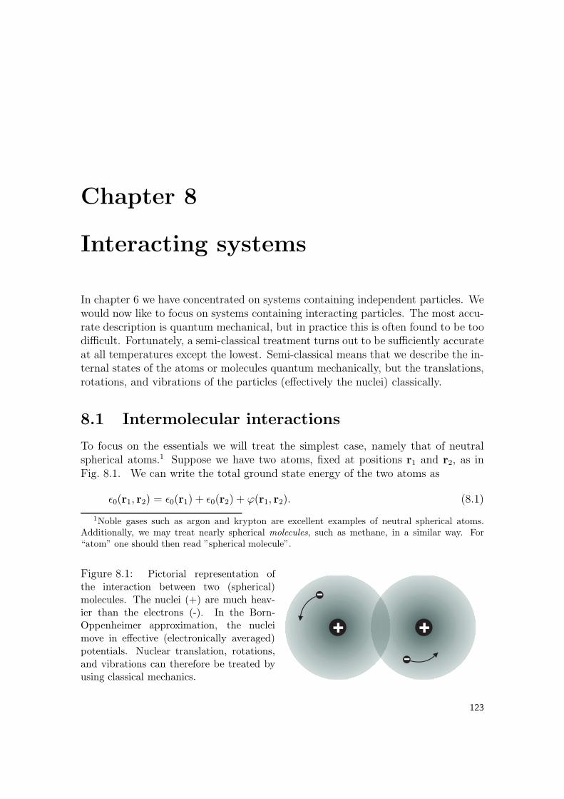
To focus on the essentials we will treat the simplest case, namely that of neutralspherical atoms.1 Suppose we have two atoms, fixed at positions r1 and r2, as inFig. 8.1. We can write the total ground state energy of the two atoms as

ǫ0(r1, r2) = ǫ0(r1) + ǫ0(r2) + ϕ(r1, r2). (8.1)

1Noble gases such as argon and krypton are excellent examples of neutral spherical atoms.Additionally, we may treat nearly spherical molecules, such as methane, in a similar way. For“atom” one should then read ”spherical molecule”.

Figure 8.1: Pictorial representation ofthe interaction between two (spherical)molecules. The nuclei (+) are much heav-ier than the electrons (-). In the Born-Oppenheimer approximation, the nucleimove in effective (electronically averaged)potentials. Nuclear translation, rotations,and vibrations can therefore be treated byusing classical mechanics.

123

8. INTERACTING SYSTEMS

0.5 1.0 1.5 2.0 2.5r/σ

-1

0

1

2

ϕ(r)

/ε

van der Waals attraction

Pauli repulsion

r = σ

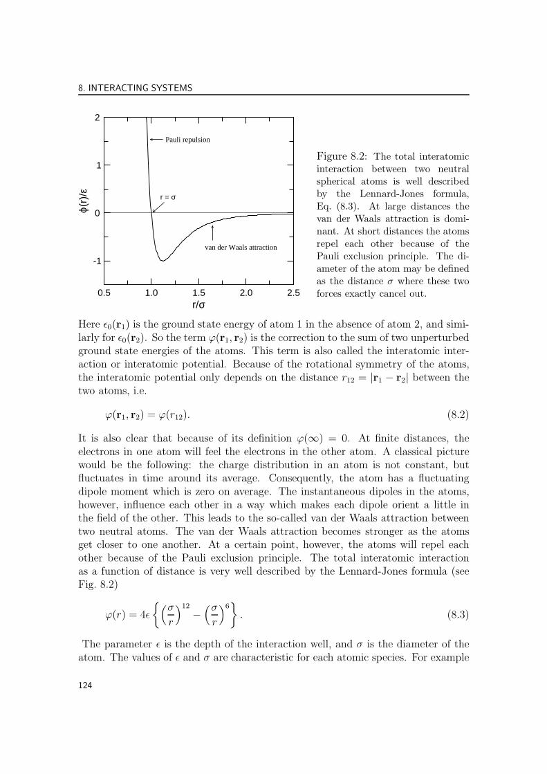
Figure 8.2: The total interatomicinteraction between two neutralspherical atoms is well describedby the Lennard-Jones formula,Eq. (8.3). At large distances thevan der Waals attraction is domi-nant. At short distances the atomsrepel each other because of thePauli exclusion principle. The di-ameter of the atom may be definedas the distance σ where these twoforces exactly cancel out.

Here ǫ0(r1) is the ground state energy of atom 1 in the absence of atom 2, and simi-larly for ǫ0(r2). So the term ϕ(r1, r2) is the correction to the sum of two unperturbedground state energies of the atoms. This term is also called the interatomic inter-action or interatomic potential. Because of the rotational symmetry of the atoms,the interatomic potential only depends on the distance r12 = |r1 − r2| between thetwo atoms, i.e.

ϕ(r1, r2) = ϕ(r12). (8.2)

It is also clear that because of its definition ϕ(∞) = 0. At finite distances, theelectrons in one atom will feel the electrons in the other atom. A classical picturewould be the following: the charge distribution in an atom is not constant, butfluctuates in time around its average. Consequently, the atom has a fluctuatingdipole moment which is zero on average. The instantaneous dipoles in the atoms,however, influence each other in a way which makes each dipole orient a little inthe field of the other. This leads to the so-called van der Waals attraction betweentwo neutral atoms. The van der Waals attraction becomes stronger as the atomsget closer to one another. At a certain point, however, the atoms will repel eachother because of the Pauli exclusion principle. The total interatomic interactionas a function of distance is very well described by the Lennard-Jones formula (seeFig. 8.2)

ϕ(r) = 4ǫ

(σr

)12

−(σr

)6. (8.3)

The parameter ǫ is the depth of the interaction well, and σ is the diameter of theatom. The values of ǫ and σ are characteristic for each atomic species. For example

124


for argon ǫ/kB = 117.7 K and σ = 0.3504 nm, for krypton ǫ/kB = 164.0 K andσ = 0.3827 nm, and for methane ǫ/kB = 148.9 K and σ = 0.3783 nm. We note thatthe magnitudes of ǫ are much lower than the magnitude of the ground state energyǫe0 of the electronically averaged potential between two covalently bound atoms in atwo-atomic molecule, as in section 6.3 and Fig. 6.1. Of course, in the case of two-atomic molecules there are also van der Waals attractions between the (non-bonded)atoms on different molecules. These interactions have been ignored in chapter 6,but may be included in a way similar to the following treatment.

We are now going to calculate the total energy of a system of N particles (atomsor molecules) in the semi-classical approximation. This means that we need to addterms representing the kinetic energy explicitly. Regarding the potential energy, forsimplicity we are going to assume that it may be approximated as a sum of pairinteractions (in practice this is often a reasonable assumption):

Φ (r1, . . . , rN) =

N−1∑

i=1

N∑

j=i+1

ϕ(rij). (8.4)

The double sum is constructed such that each pair interaction is counted only once.The total energy can then be expressed as

E =N∑

i=1

1

2m

(p2

xi + p2yi + p2

zi

)+Nǫ0 + Φ (r1, . . . , rN) . (8.5)

Here pxi = mvxi is the x-component of the momentum of particle i.

8.2 The semi-classical partition function

To make use of the statistical mechanical machinery developed in the previous chap-ters, we need to be able to specify the state of the system in a countable number ofways. The state may be specified by providing N numbers nxi, N numbers nyi, Nnumbers nzi, and similarly for mxi to mzi, such that the positions and momenta ofthe particles are given by

nxi∆x < rxi ≤ (nxi + 1)∆x

nyi∆x < ryi ≤ (nyi + 1)∆x

nzi∆x < rzi ≤ (nzi + 1)∆x

mxi∆p < pxi ≤ (mxi + 1)∆p

myi∆p < pyi ≤ (myi + 1)∆p

mzi∆p < pzi ≤ (mzi + 1)∆p

125


∆x and ∆p may be interpreted as the precision with which we are able to specifythe position and momentum of a particle. If we combine all these integer numbersinto one index n, we can calculate the probability to encounter the system in staten, analogous to our treatment chapter 7. In the canonical ensemble we have

Pn =1

Q′exp −βEn (8.6)

Q′ =∑

n

exp −βEn , (8.7)

where we have labeled the partition function as Q′, to distinguish it from the quan-tum mechanical partition function Q. If we now further write out Q′, ignoring theconstant internal energy Nǫ0, we find

Q′ =∑

nx1

. . .∑

nzN

∑

mx1

. . .∑

mzN

exp

−β

∑

i

1

2m

(p2

xi + p2yi + p2

zi

)− βΦ (r1, . . . , rN)

=1

(∆x∆p)3N

∫dpx1 . . .

∫dpzN

∫drx1 . . .

∫drzN

× exp

−β

∑

i

1

2m

(p2

xi + p2yi + p2

zi

)− βΦ (r1, . . . , rN)

=(2πmkBT )3N/2

(∆x∆p)3N

∫drx1 . . .

∫drzN exp −βΦ (r1, . . . , rN)

=(2πmkBT )3N/2

(∆x∆p)3NZ, (8.8)

where

Z ≡∫

drx1 . . .∫

drzN exp −βΦ (r1, . . . , rN) . (8.9)

The integrals in Z must be taken over the entire system’s volume. Z is called theconfiguration integral or configuration sum-of-states.

We continue reasoning as in section 7.1.2. The average energy 〈E〉 must be equalto the thermodynamic energy U , therefore

(∂A/T

∂1/T

)

N,V

= U = 〈E〉 = −kB

(∂ lnQ′

∂1/T

)

N,V

. (8.10)

Integrating we find

A

T= −kB lnQ′ − S0 (8.11)

A = −kBT ln(eS0/kBQ′

). (8.12)

126


S0 is nothing but an integration constant fixing the zero point of entropy. Let usnow try to find an S0 such that

Qclas = eS0/kBQ′ = Qquant, (8.13)

i.e. such that the semi-classical partition function agrees with the quantum me-chanical result. We can easily do this for the case of an ideal gas. The quantummechanical partition function of an ideal gas is given by Eqs. (5.30) and (5.31):

Qquant =

(2πmkBT

h2

)3N/21

N !V N . (8.14)

Semi-classically, because Φ = 0 for an ideal gas, we have for the configurationintegral

Z =

∫drx1 . . .

∫drzN 1 = V N , (8.15)

and therefore

Qclas = eS0/kB(2πmkBT )3N/2

(∆x∆p)3NV N . (8.16)

Equating we find

eS0/kB =

(∆x∆p

h

)3N1

N !. (8.17)

In summary, the (semi-)classical statistical physics of a system in the canonicalensemble may be described by the following three equations:

A = −kBT lnQ (8.18)

Q = eS0/kBQ′ =

(2πmkBT

h2

)3N/21

N !Z (8.19)

Z =

∫d3Nr e−βΦ(r3N ), (8.20)

where we have used the abbreviated form d3Nr = drx1 . . . drzN .

An alternative derivation for the appearance of the factor 1/h3N is given in theAppendix of this chapter.

127


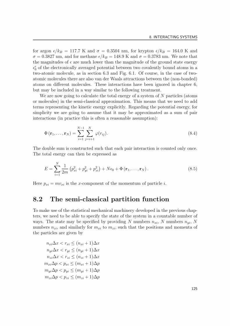
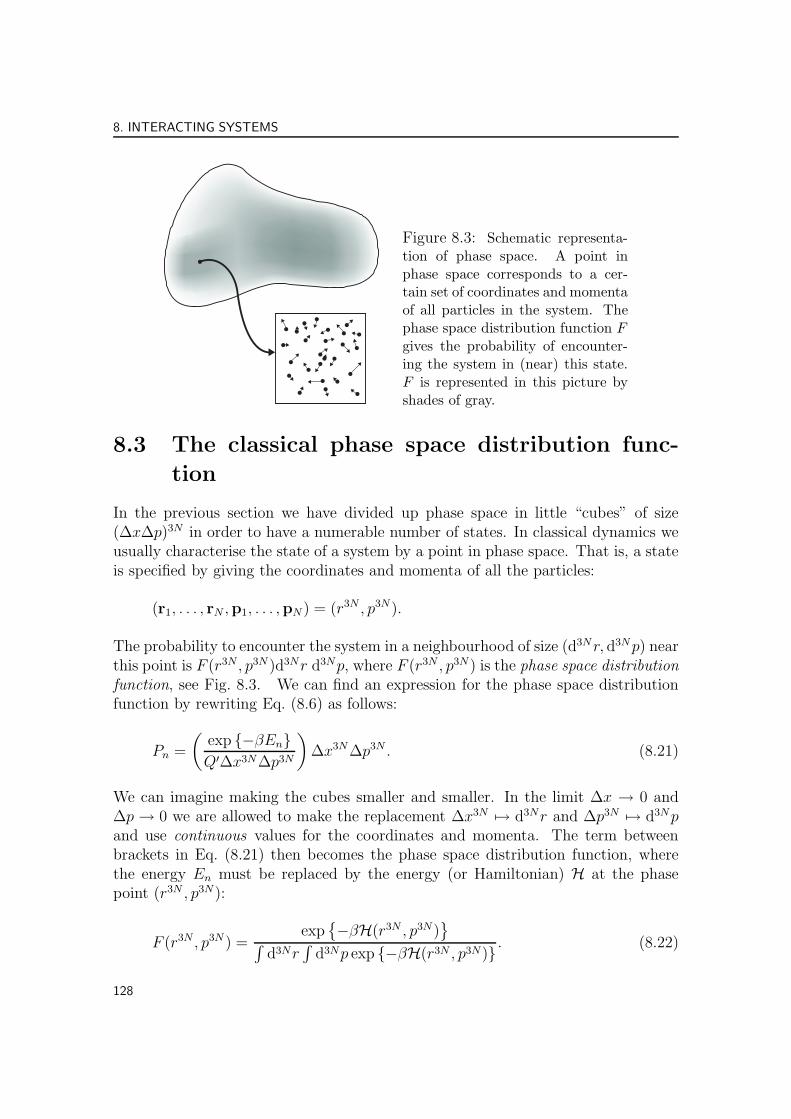
Figure 8.3: Schematic representa-tion of phase space. A point inphase space corresponds to a cer-tain set of coordinates and momentaof all particles in the system. Thephase space distribution function F

gives the probability of encounter-ing the system in (near) this state.F is represented in this picture byshades of gray.

8.3 The classical phase space distribution func-

tion

In the previous section we have divided up phase space in little “cubes” of size(∆x∆p)3N in order to have a numerable number of states. In classical dynamics weusually characterise the state of a system by a point in phase space. That is, a stateis specified by giving the coordinates and momenta of all the particles:

(r1, . . . , rN ,p1, . . . ,pN ) = (r3N , p3N).

The probability to encounter the system in a neighbourhood of size (d3Nr, d3Np) nearthis point is F (r3N , p3N )d3Nr d3Np, where F (r3N , p3N) is the phase space distribution

function, see Fig. 8.3. We can find an expression for the phase space distributionfunction by rewriting Eq. (8.6) as follows:

Pn =

(exp −βEnQ′∆x3N∆p3N

)∆x3N∆p3N . (8.21)

We can imagine making the cubes smaller and smaller. In the limit ∆x → 0 and∆p → 0 we are allowed to make the replacement ∆x3N 7→ d3Nr and ∆p3N 7→ d3Npand use continuous values for the coordinates and momenta. The term betweenbrackets in Eq. (8.21) then becomes the phase space distribution function, wherethe energy En must be replaced by the energy (or Hamiltonian) H at the phasepoint (r3N , p3N):

F (r3N , p3N ) =exp

−βH(r3N , p3N)

∫

d3Nr∫

d3Np exp −βH(r3N , p3N) . (8.22)

128


Note that F is properly normalised, i.e.∫

d3Nr

∫d3Np F (r3N , p3N) = 1, (8.23)

as is required for a probability distribution function.From Eq. (8.5) we observe that the (semi-)classical Hamiltonian consists of two

parts, a kinetic part K(p3N) which only depends on the momenta and a potentialpart Φ(r3N) which only depends on the coordinates. Therefore the phase spacedistribution function factors as (prove this!)

F (r3N , p3N ) = F r(r3N)F p(p3N), (8.24)

where

F r(r3N) =exp

−βΦ(r3N)

∫

d3Nr exp −βΦ(r3N ) =1

Zexp

−βΦ(r3N )

(8.25)

is the probability distribution for observing the system at configuration space pointr3N , and

F p(p3N) =exp

−βK(p3N)

∫

d3Np exp −βK(p3N) (8.26)

is the probability distribution for observing the system at momentum space pointp3N .

We can factor the momentum distribution some more, since the kinetic energyis a sum of N single particle energies

∑i p

2i /2m:

F p(p3N) =

N∏

i=1

f p(pi), (8.27)

where

f p(pi) =exp −βp2

i /2m∫d3p exp −βp2/2m . (8.28)

More explicitly, performing the integral, we find the single particle momentum dis-tribution

f p(px, py, pz) =

(1

2πmkBT

)3/2

exp

− 1

2mkBT

(p2

x + p2y + p2

z

). (8.29)

This is called the Maxwell-Boltzmann momentum distribution. It applies to allsemi-classical systems at temperature T , i.e. not only to ideal gases, but also to

129


non-ideal gases, liquids, and solids. As a consequence the average absolute velocityof a particle is the same in a liquid and a gas, provided the temperature is thesame. Of course, the frequency of collisions in a liquid is much higher than that ina gas. That is why a molecule will travel much further per second in a gas than in acondensed phase even though the single molecule velocity distributions are identicalin the two phases.

Note that the average momentum 〈px〉 predicted by Eq. (8.29) is zero. Its secondmoment 〈p2

x〉, however, is not zero. In fact, it is easy to show that the average kineticenergy per particle (in three dimensional space) is given by (Problem 8-1)

〈K〉 /N =1

2m

⟨p2

x + p2y + p2

z

⟩=

3

2kBT. (8.30)

We will use this in section 8.4 to measure the temperature in a molecular dynamicssimulation. Note that for an ideal gas the kinetic energy is the only energy termpresent (because Φ = 0). Thus we confirm the result U = 〈K〉 = 3

2NkBT for an

ideal gas.

Eq. (8.30) is an example of the more general equipartition theorem, which statesthat for a classical system each quadratic term in the Hamiltonian will, on average,“receive” an energy of 1

2kBT . So besides terms such as p2

xi/2m, also terms such asmω2x2/2 will have an average energy of 1

2kBT .

8.4 Molecular dynamics simulations

8.4.1 “Experimental” statistical physics

Numerical simulations are the “experimental” tool of statistical physicists. Such atool is absolutely necessary because the interactions between particles are usuallytoo complex to allow a theoretical analysis of the macroscopic system properties.The analytically solvable models we have encountered up to now, such as the idealgas and the harmonic crystal, are rare exceptions.

In this chapter we will introduce the molecular dynamics (MD) simulation tech-nique. MD enables us to calculate structural and thermodynamic properties, aswell as dynamical properties, of realistic molecular systems, provided they excludechemical reactions and other phenomena of a quantum mechanical nature. There isanother important technique, called Monte Carlo (MC) simulation, which enablesus to efficiently sample the phase space in a specified ensemble. This also yieldsstructural and thermodynamic properties, but no dynamical properties. We willnot treat the Monte Carlo technique here.

130


8.4.2 Force fields

Usually one simulates a box containing a number of N particles (atoms). The totalpotential energy Φ is usually divided up into terms depending on the coordinates ofindividual particles, pair, triplets, etc.

Φ =∑

i

ϕ1(ri) +∑

i

∑

j>i

ϕ2(ri, rj) +∑

i

∑

j>i

∑

k>j

ϕ3(ri, rj, rk) + . . . (8.31)

The first term in Eq. (8.31) represents the effect of an external field on the sys-tem. The remaining terms represent particle interactions. Non-bonded interactionsbetween atoms are usually described by a Lennard-Jones potential, as we encoun-tered in section 8.1, supplemented with Coulombic terms if the atoms are charged.Bonded interactions within molecules typically consist of a harmonic potential be-tween two bonded atoms, a bending potential for three consecutively bonded atoms,and a dihedral potential for four consecutively bonded atoms.

In its simplest implementation, the molecular dynamics method generates a pathon a constant energy surface in phase space, H(rN ,pN) = U , by solving Newton’sequations of motion for all the particles. According to Newton, the force on eachparticle leads to an acceleration given by

mid2ri

dt2= −∇iΦ(rN). (8.32)

Since Newton’s equations are second order equations, the paths of all particles arecompletely determined once the initial positions and initial velocities are given.

8.4.3 Numerical integration

How should we solve Eq. (8.32) on a computer? In order to concentrate on essentialpoints, we simplify our notation for the time being and restrict ourselves to just onedegree of freedom. Then we may write

dx

dt= v, (8.33)

dv

dt=

F

m, (8.34)

where F = −dΦ/dx is the force acting on this particular coordinate. The simplestsolution to this problem is

x (t+ ∆t) = x (t) + v (t) ∆t, (8.35)

v (t+ ∆t) = v (t) +F (t)

m∆t, (8.36)

131


0 20 40 60 80 100time

0.4

0.6

0.8

1.0

1.2

1.4

tota

l ene

rgy

E

EulerVerlet

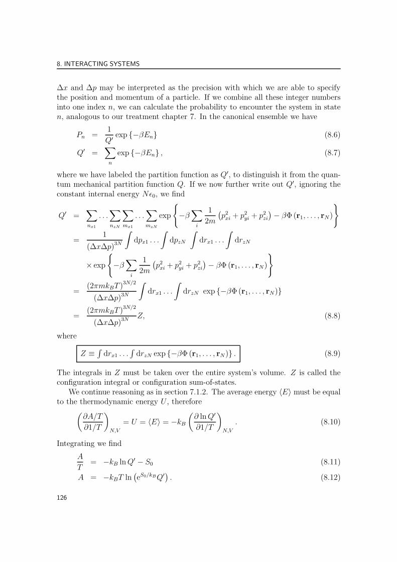
Harmonic oscillator

m = ω = 1

x0 = 1, v

0 = 0

∆t = 0.01

Figure 8.4: Total energy of aharmonic oscillator E = Φ +K with K = 1

2mv2 and Φ =12mω2x2. In this example wehave chosen m = 1 and ω = 1.Results are given for integrationwith the Euler algorithm (solidline) and Verlet leap-frog algo-rithm (dashed line), both with atime step of ∆t = 0.01. Note thatthe period (time for one oscilla-tion) is 2π.

which must be repeated as often as needed to reach the time of interest. Thisalgorithm is called the first order Euler algorithm. Applying it to the simple case ofa harmonic oscillator reveals that this algorithm does not conserve energy; actuallythe error of the energy grows exponentially with time, see Fig. 8.4.

An astonishingly simple solution to the above problem is to write:

x (t+ ∆t) = x (t) + x (t) ∆t+1

2x (t) (∆t)2 +

1

6

···

x (t) (∆t)3 + . . . , (8.37)

x (t− ∆t) = x (t) − x (t) ∆t+1

2x (t) (∆t)2 − 1

6

···

x (t) (∆t)3 + . . . . (8.38)

After adding these two equations we obtain

x (t+ ∆t) = 2x (t) − x (t− ∆t) + x (t) (∆t)2 + O(∆t4). (8.39)

This propagator is correct to order (∆t)4. Instead of the position and velocity bothat time t, we need the positions at time t and at time t − ∆t in order to advancethe system by ∆t. The price we pay for the better algorithm is that it doesn’t lookvery nice, so let’s make it look nicer. To this end we introduce new names

x (t) − x(t− ∆t) = v

(t− 1

2∆t

)∆t, (8.40)

x (t+ ∆t) − x(t) = v

(t+

1

2∆t

)∆t. (8.41)

For the time being these equations only serve to define the new symbols v(t− 1

2∆t

)

132


and v(t+ 1

2∆t

). The propagator now reads

v

(t+

1

2∆t

)= v

(t− 1

2∆t

)+F (t)

m∆t. (8.42)

x (t+ ∆t) = x (t) + v

(t+

1

2∆t

)∆t, (8.43)

The second line is nothing but repeating Eq. (8.41), while the first line is Eq. (8.39)rewritten in our new notation. Consequently the algorithm still is correct up tofourth order in ∆t. It is called the Verlet leap-frog algorithm.

Obviously we now would like to know about velocities. From an analysis similarto the one just given we deduce that the velocity x(t) at time t is given by theobvious equation

x (t) =1

2

v

(t+

1

2∆t

)+ v

(t− 1

2∆t

), (8.44)

correct to second order in ∆t. It is important to stress again that this does notinfluence the propagator, which is correct to fourth order. For small enough time-steps ∆t, the Verlet algorithm performs an excellent job at conserving total energy,see Fig. 8.4.

Extension of this method to a system with 3N Cartesian coordinates is trivial.

8.4.4 Bulk systems and periodic boundary conditions

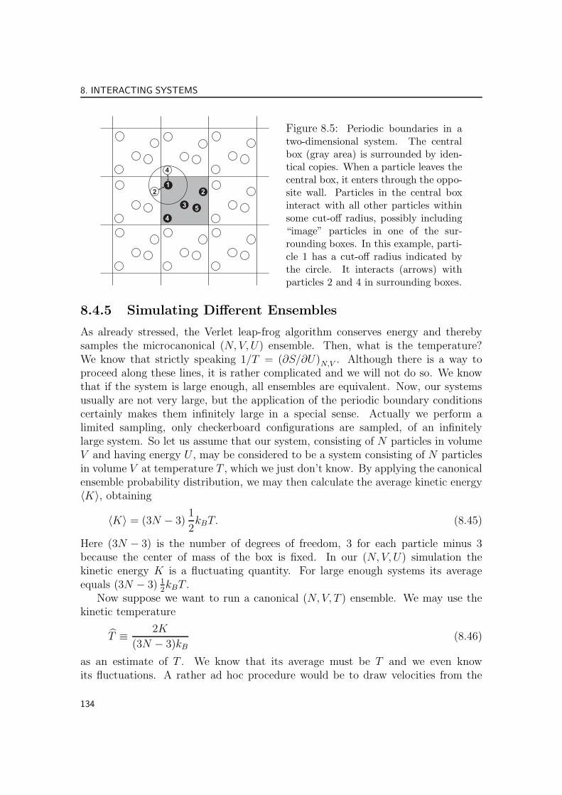
Often we are interested in the bulk properties of a certain material. Bulk systems aremacroscopically large and consist of 1020 particles or more, while simulation boxesare limited to about 106 particles, but usually consist of 100 000 or less particles. Insuch small boxes most particles will be close to the system boundary and thereforenot behave as a bulk particle at all. This problem is alleviated by the use of periodicboundary conditions, see Fig. 8.5.

First the simulation box is surrounded in all directions by copies of itself. Noticethat we only have to keep track of the positions of the particles in the central boxand that we then automatically know the positions of the particles in the otherboxes. Next we do two things. (1) We remove the confining boundaries. Thus, eachparticle which leaves the central box automatically enters this box through the wallopposite the one through which it left the box. (2) We let each particle interact withall other particles within a certain cut-off radius, possibly including particles in oneof the surrounding boxes. The cut-off radius is limited by the fact that we do notwant a particle to interact with one of its own images. An even stronger restrictionis that we do not want a particle to interact with a second particle and at the sametime with some copy of this second particle. In this case the cut-off radius is at mostL/2 with L the length of an edge of a cubic box.

133


Figure 8.5: Periodic boundaries in atwo-dimensional system. The centralbox (gray area) is surrounded by iden-tical copies. When a particle leaves thecentral box, it enters through the oppo-site wall. Particles in the central boxinteract with all other particles withinsome cut-off radius, possibly including“image” particles in one of the sur-rounding boxes. In this example, parti-cle 1 has a cut-off radius indicated bythe circle. It interacts (arrows) withparticles 2 and 4 in surrounding boxes.

8.4.5 Simulating Different Ensembles

As already stressed, the Verlet leap-frog algorithm conserves energy and therebysamples the microcanonical (N, V, U) ensemble. Then, what is the temperature?We know that strictly speaking 1/T = (∂S/∂U)N,V . Although there is a way toproceed along these lines, it is rather complicated and we will not do so. We knowthat if the system is large enough, all ensembles are equivalent. Now, our systemsusually are not very large, but the application of the periodic boundary conditionscertainly makes them infinitely large in a special sense. Actually we perform alimited sampling, only checkerboard configurations are sampled, of an infinitelylarge system. So let us assume that our system, consisting of N particles in volumeV and having energy U , may be considered to be a system consisting of N particlesin volume V at temperature T , which we just don’t know. By applying the canonicalensemble probability distribution, we may then calculate the average kinetic energy〈K〉, obtaining

〈K〉 = (3N − 3)1

2kBT. (8.45)

Here (3N − 3) is the number of degrees of freedom, 3 for each particle minus 3because the center of mass of the box is fixed. In our (N, V, U) simulation thekinetic energy K is a fluctuating quantity. For large enough systems its averageequals (3N − 3) 1

2kBT .

Now suppose we want to run a canonical (N, V, T ) ensemble. We may use thekinetic temperature

T ≡ 2K

(3N − 3)kB(8.46)

as an estimate of T . We know that its average must be T and we even knowits fluctuations. A rather ad hoc procedure would be to draw velocities from the

134


Maxwell-Boltzmann distribution for the initial velocities and subsequently to rescaleall velocities at every time step by a factor

χ =

√

1 +∆t

τ

(T

T− 1

). (8.47)

This will change the kinetic temperature T every time-step according to

T −→ T

[1 +

∆t

τ

(T

T− 1

)]. (8.48)

If the characteristic time τ is chosen to be equal to ∆t this algorithm forces T to beequal to T at all times and we loose the natural fluctuations of the kinetic energy.Therefore τ is chosen by trial and error to be such that the fluctuations of thekinetic energy are about right. The procedure just described is usually referred toas applying the Berendsen thermostat. An alternative is the so-called Nose-Hooverthermostat, which steers the temperature towards the required value in a muchgentler way and correctly generates states in the canonical ensemble.

Other ensembles may be simulated as well. For example, to control the pressureP , the system box is allowed to change its volume during the simulation.

8.4.6 Limitations

The computational demands of molecular dynamics, the interaction forces betweenevery atom and its 25 to 50 nearest neighbours must be recalculated every timestep, puts restrictions on the accessible length and time scales. A typical simulationbox used for simulation of a liquid has edges of the order of 10 nm and containssome 100 000 atoms, though occasionally even larger boxes are being used. Theevaluation of a single time step then takes about a second of computer time, whichis predominantly spent on the calculation of the non-bonded interactions betweenthe atoms. With time steps in the order of a femtosecond (10−15 s), a week ofcomputer time corresponds to about a nanosecond (10−9 s) in real time. Of course,these numbers will vary considerably depending on the details of the system, theforce field (where in particular long-range Coulombic interactions are demanding),the efficiency of the algorithm, and the available hardware.

The above discussion clearly illustrates that the capabilities of atomistic molec-ular dynamics simulations are limited, yet even within these boundaries interestingphysical phenomena can be studied. In fact, by taking full advantage of the prin-ciples of statistical mechanics, it is possible to extract thermodynamic, structural,and dynamic properties from relatively small simulation boxes.

135


Appendix

In this Appendix we will give an alternative derivation of the classical partitionfunction Q, starting from a quantum mechanical description. For simplicity weconsider just one particle in one dimension. The partition function is a sum ofBoltzmann factors over all possible (energy) states:

Q =∑

n

e−βEn

=∑

n

⟨ψn|e−βH|ψn

⟩, (8.49)

where ψn is an eigenstate of the Hamilton operator H of energy (eigenvalue) En, i.e.Hψn = Enψn. Note that the exponential of an operator A, operating on a functionf is defined in terms of the equivalent Taylor series:

eAf =

∞∑

k=0

1

k!Akf = f + Af +

1

2A(Af) +

1

6A(A(Af)) + . . . (8.50)

We now proceed as follows. The sum in the second line of Eq. (8.49) defines thetrace of the operator e−βH over the complete basis set of eigenfunctions ψn. Becausethe trace is invariant under exchange of complete basis sets, we may as well chooseany other complete basis φn, resulting in the same partition function:

Q =∑

n

⟨φn|e−βH|φn

⟩. (8.51)

We now choose the particular (complete) basis

φn(x) =1√L

ei2πnx/L, (8.52)

where L is the space accessible to the particle.Note that the Hamilton operator consists of a kinetic and potential energy op-

erator, H = K + Φ, where usually the kinetic operator depends on the momentump = ~

iddx

and the potential operator depends on the position x. It is well known fromquantum mechanics that the momentum and position of a particle do not commute,specifically [p, x] = ~/i. Therefore the kinetic and potential energy operators alsodo not commute, [K,Φ] 6= 0, and we cannot simply factorize the operator e−βH:

e−β(K+Φ) 6= e−βKe−βΦ. (8.53)

However, in the classical limit we can regard ~ as very small, and we do have

e−β(K+Φ) ≈ e−βKe−βΦ ≈ e−βΦe−βK (classical limit). (8.54)

136


So in the classical limit we can write the partition function as:

Q =∑

n

∫ L

0

dx1√L

e−i2πnx/Leβ ~2

2md2

dx2 e−βΦ(x) 1√L

ei2πnx/L

=∑

n

∫ L

0

dx1

Le−β 1

2m(~2πn/L)2e−βΦ(x)

=

∫∞

−∞

dpL

~2π

∫ L

0

dx1

Le−β p2

2m−βΦ(x)

=1

h

∫dp

∫dx e−βH. (8.55)

This is the result we were after. Generalisation to 3N coordinates and 3N momentaleads to the expression

Q =1

h3NN !

∫d3Np

∫d3Nx e−βH, (8.56)

where the factor N ! appears because of indistinguishability of identical particles. Itis easy to check that Eq. (8.56) is equivalent to Eq. (8.19).

137


Problems

8-1. Average kinetic energy per particle. Prove Eq. (8.30). Then calculatethe r.m.s. velocity

√〈v2〉 of a nitrogen molecule in the air at room temperature.

8-2. Barometric height formula. The density ρα = Nα/V of a certain moleculeα in a column of air above the earth surface decreases with increasing height. If wedenote the height above earth with z, we find

ρα(z) = ρα(0) exp

(−mαgz

kBT

),

where g is the gravitational constant and mα the mass of the molecule. Prove this.(You may assume that the temperature is constant everywhere and that the airbehaves as an ideal gas.)

8-3. Gravitational energy of an ideal gas particle above the earth surface.Consider again a column of air above the earth surface. Using the outcome of theprevious problem, the single-particle probability density of encountering a particleof mass m at position r with a momentum p is given by

F (r,p) = C exp

(−mgzkBT

)exp

(− p2

2mkBT

).

where C is a normalisation constant. Calculate the average gravitational energymg 〈z〉 of the particle.

138

Chapter 9

Non-ideal gasses and liquids

In real liquids and gases there are correlations in the positions of the molecules. Theaim of almost all modern theories of liquids is to calculate the radial distributionfunction by means of statistical thermodynamical reasoning. Alternatively, the ra-dial distribution function can be measured directly in computer simulations. Wewill discuss its use in calculating the energy and pressure of a fluid. We will alsobriefly discuss its use in perturbation theory for the free energy. We show how theconfiguration integral and pressure can be calculated by a diagrammatic expansionmethod. Finally, we introduce the use of lattice models to facilitate the calculationof the free energy and pressure of fluids and mixtures.

9.1 The radial distribution function

9.1.1 Definition

Imaging we have placed ourselves on a certain molecule in a liquid or gas. Now letus count the number of molecules in a spherical shell of thickness dr at a distancer, i.e. we count the number of molecules within a distance between r and r + dr.If r is very large the measured number of molecules will be equal to the volume ofthe spherical shell times the density, so equal to 4πr2drN/V . At distances smallerthan the diameter of the molecules we will find no molecules at all. We now definethe radial distribution function g(r) by equating the number of molecules in thespherical shell of thickness dr at a distance r to

4πr2N

Vg(r)dr. (9.1)

According to our remarks above, g(∞) = 1 and g(0) = 0. A typical g(r) is given inFig. (9.1). We see that g(r) = 0 when r is smaller than the molecular diameter σ.The first peak is caused by the attractive part of the potential; at distances where

139

9. NON-IDEAL GASSES AND LIQUIDS

r

g(r)

1

σ

Figure 9.1: A typical ra-dial distribution function in aliquid of spherical moleculeswith diameter σ.

the potential has its minimum there are more particles than average. Consequentlyat distances less than σ further away there are less particles than average.

9.1.2 Relation between g(r) and energy, compressibility andpressure

Once we know the radial distribution function, we can derive all non-entropic ther-modynamic properties. The simplest is the energy

U = U int +3

2NkBT +

1

2NN

V

∫∞

0

dr4πr2g(r)ϕ(r). (9.2)

The first term originates from the internal energies of the molecules, the second fromthe translations, and the third from the interactions. The average total potentialenergy equals 1

2N times the average interaction of one particular molecule with all

others; the factor 12

serves to avoid double counting. The contribution of all particlesin a spherical shell of thickness dr at a distance r to the average interaction of oneparticular particle with all others is 4πr2dr(N/V )g(r)ϕ(r). Integration finally yieldsEq. (9.2).

We can also calculate the compressibility κT . This is done as follows (whereagain ρ = N/V is the particle number density and d3r is shorthand for 4πr2dr):

〈N〉 ρkBTκT =⟨N2

⟩− 〈N〉2

=

⟨ρ

∫

V

d3r1ρ

∫

V

d3r2g(r12)

⟩+ 〈N〉 −

⟨ρ

∫

V

d3r1ρ

∫

V

d3r2

⟩

=

⟨ρ

∫

V

d3r1ρ

∫

V

d3r2 (g(r12) − 1)

⟩+ 〈N〉

=

⟨ρ

∫

V

d3r1ρ

∫

R3

d3r2 (g(r12) − 1)

⟩+ 〈N〉

=

⟨ρ

∫

V

d3r1

⟩ ⟨ρ

∫

R3

d3r (g(r) − 1)

⟩+ 〈N〉 (9.3)

140


Dividing by 〈N〉 we find

ρkBTκT =

⟨ρ

∫

R3

d3r (g(r)− 1)

⟩+ 1. (9.4)

This shows that the compressibility of a fluid is intimately connected to the radialdistribution function of its constituent molecules.

We will now consider the pressure of a non-ideal fluid. If the density of the fluidis not too high the radial distribution function is given by

g(r) ≈ exp −βϕ(r) , (9.5)

where ϕ(r) is the pair interaction potential. We can link the pressure of such a semi-dilute system to the pair interaction ϕ(r), and hence to its g(r), in the followingway.

For not too high densities we may terminate the virial equation Eq. (2.62) afterthe second term, i.e., the pressure of a semi-dilute fluid is to a good approximationgiven by

Pv = RT

(1 +B2(T )

1

v

). (9.6)

This implies a connection between the compressibility and the second virial coeffi-cient B2(T ). Differentiating the above equation to v yields:

(∂P

∂v

)

N,T

v + P = −RTB2(T )1

v2

− 1

κT+RT

v

(1 +B2(T )

1

v

)= −RTB2(T )

1

v2

1

κT

=RT

v

(1 + 2B2(T )

1

v

)

ρkBTκT = 1 − 2B2(T )1

v, (9.7)

where we have used that ρ = N/V = NAv/v. Comparing the two expressions forthe compressibility, Eqs. (9.4) and (9.7), we can write the second virial coefficientas a three-dimensional integral over the pair interaction ϕ(r):

B2(T ) = −1

2NAv

∫

R3

d3r(e−βϕ(r) − 1

). (9.8)

The above equation is very important because it allows us to calculate the pressureof a fluid knowing only the pair interaction ϕ(r) between its constituent molecules.In the next section we will apply this to a hard sphere fluid.

141


9.2 The hard sphere fluid

The second virial coefficient B2 of a hard sphere fluid (with spheres of diameter σ)can easily be calculated

B2 = −1

2NAv

∫d3r

(e−βϕ(r) − 1

)= 2πNAv

∫ σ

0

drr2 =2

3πNAvσ

3. (9.9)

This expression is valid for not-too-high densities. Using a computer one has calcu-lated that the pressure for more general densities is given by:

P

ρkBT= 1 + 4η + 10η2 + 18.365η3 + 28.24η4 + 39.5η5 + 56.6η6 + . . . (9.10)

η =4

3π(

1

2σ)3N

V, (9.11)

where η is the volume fraction of spheres. We can write approximately

P

ρkBT= 1 + 4η + 10η2 + 18η3 + 28η4 + 40η5 + 54η6 + . . . (9.12)

Extrapolating and summing we find

P

ρkBT= 1 +

∞∑

n=1

(n2 + 3n)ηn =1 + η + η2 − η3

(1 − η)3. (9.13)

This is called Carnahan and Starling’s equation for the pressure of a hard spherefluid. Monte Carlo simulations of hard sphere fluids have shown that Eq. (9.13) isnearly exact at all possible volume fractions.

The entropy of a non-ideal gas is mostly determined by the repulsive part of thepotential energy, because this part of the potential determines the number of statesthat contributes to the configuration integral. The entropy of a hard sphere fluidmay therefore serve as a first approximation to the entropy of any fluid with sphericalparticles. The free energy of the hard sphere fluid, and concordingly all thermody-namic properties, can be calculated from P = −(∂A/∂V )T . Using Eq. (9.13) wefind

AHS = −NkBT ln

(qinte

Λ3

V

N

)+NkBT

η(4 − 3η)

(1 − η)2, (9.14)

where qint is the one-particle partition function of the internal degrees of freedomof the molecule. This formula plays an important role in perturbation theory whichwe will briefly discuss in the next section.

142


9.3 Perturbation theory

In this section we will briefly schetch a very important technique, called perturbationtheory. In perturbation theory we write the pair interaction as

ϕ(r) = ϕ0(r) + ϕ′(r). (9.15)

A good choice is one in which ϕ0(r) is the repulsion and ϕ′(r) the attraction. Thefree energy calculated with only ϕ0(r) we will call A0. To a good approximation thefollowing expression is valid:

A = A0 +1

2NN

V

∫∞

0

dr4πr2g0(r)ϕ′(r). (9.16)

If we choose, as above, for ϕ0(r) the repulsive part of the potential, then A0 will begiven by AHS in Eq. (9.14). g0(r) is the radial distribution function of the ‘referencesystem’ with interaction ϕ0(r). If we take for ϕ0(r) a hard core repulsion, then g0(r)is the radial distribution function of a hard sphere fluid; this function is well knownfrom Monte Carlo simulations. Formula (9.16) leads to excellent predictions.

Using perturbation theory we may derive Van der Waals’ equation of state. Tothis end we add the following additional approximation:

gHS(r) = 0 for r < σ

= 1 for r ≥ σ

AHS = −NkBT ln

(qinte

Λ3

V

N

)−NkBT ln(1 − 4η) (9.17)

The free energy of the system then becomes

A = −NkBT ln

(qint

Λ3

e

N

)−NkBT ln(V − nb) − a

n2

V, (9.18)

with

a = −1

2N2

av4π

∫∞

σ

drr2ϕ(r),

b =2

3πσ3Nav. (9.19)

Because ϕ(r) < 0 for r > σ the constant a is positive.

143


9.4 Relation between fugacity and the configura-

tion integral

The intermolecular interactions in a non-ideal system contribute to all thermody-namic properties. In this section we will focus on the fugacity and fugacity coeffi-cient. According to section 3.9.2 we may write the chemical potential as follows:

µ(P, T ) = µ∗(T ) +RT lnP +RT lnφ(P, T )

= µ∗(T ) +RT ln f(P, T ). (9.20)

Here φ is the fugacity coefficient and f = φP the fugacity. For an ideal gas we haveφ = 1 and f = P . So RT lnφ is the correction to ideal behaviour. We thereforeexpect a simple relation between φ and that part of the partition function Q thatdepends on the intermolecular interactions, i.e. betweeen φ and Z.

When we are dealing with molecules instead of point particles, we also need totake into account the internal states of the molecules. The semi-classical partitionfunction and free energy are then given by more general versions of Eqs. (8.18) and(8.19):

Q =(qint)

N

Λ3NN !Z, (9.21)

A = −NkBT ln

(qinte

Λ3N

)− kBT lnZN , (9.22)

where qint is the one-particle partition function of the internal degrees of free-dom of the molecule, and Λ denotes the so-called thermal De Broglie wave length√h2/(2πmkBT ). We have given Z a subscript N to indicate that Z is a function

of N . For an ideal gas we have ZN = V N . Using µ = (∂A/∂N)V,T we then easilycalculate the chemical potential. Substituting in this expression V = NkBT/P andcomparing the result with Eq. (9.20), we find for an ideal gas:

µ∗(T ) = −RT ln

(qint

Λ3kBT

). (9.23)

For a non-ideal system we find, with Eq. (8.19):

µ = −RT ln

(qint

Λ3N

)− RT ln

(∂ZN

∂N

)

V,T

= −RT ln

(qint

Λ3N

)− RT ln

ZN

ZN−1

. (9.24)

Here we have written the derivative of lnZN to N as lnZN − lnZN−1. FromEqs. (9.20), (9.23) and (9.24) follows:

lnφ = − ln

(PV

NkBT

)− ln

(1

V

ZN

ZN−1

). (9.25)

144


This is the looked-after relation between φ and Z. When applied to an ideal gas,this equation yields φ = 1, as could have been expected. For non-ideal gasses bothterms contribute.

From the treatment above follows that, as long as the partition function can bewritten as in Eq. (9.21), the chemical potential consists of a contribution µ∗ whichonly depends on the temperature and a contribution that only depends on P andT . µ∗ is totally determined by the internal states of individual molecules. The(P, T )-dependent part

ln f = − ln

(1

NkBT

ZN

ZN−1

)(9.26)

is totally determined by the configuration integral. This conclusion is valid forsystems in any state of aggregation, as long as Q may be written as in Eq. (9.21).

9.5 Diagrammatic expansions

9.5.1 The configuration integral

Let us try to calculate the configuration integral. Assume we have a system withpair interactions:

Φ(r3N) =N−1∑

i=1

N∑

j=i+1

ϕ(rij) (9.27)

Then

ZN =

∫d3r1 . . .

∫d3rN exp −βΦ(r1, . . . , rN)

=

∫d3r1 . . .

∫d3rN

N−1∏

i=1

N∏

j=i+1

exp −βϕ(rij) (9.28)

For an ideal gas we have exp −βϕ(rij) = 1. Let us now introduce the functionf(r) by

exp −βϕ(rij) = 1 + f(r) (9.29)

A qualitative picture of f(r) is given in Fig. (9.2). For a semidilute fluid it isessentially the radial distribution function shifted down by one. It is important tonote that f(r) tends to zero as r goes to infinity. The configuration integral is thengiven by

ZN =

∫d3r1 . . .

∫d3rN

N−1∏

i=1

N∏

j=i+1

(1 + f(rij)) (9.30)

145


r

f

Figure 9.2: Qualitative pic-ture of the function f(r) =exp −βϕ(rij) − 1.

Figure 9.3: One of theterms in Eq. (9.30). Aline between two moleculesmeans that the asso-ciated term contains afactor f(rij). With everychequered molecule weassociate integration of itsposition over the volume.

We need to expand the continued product and integrate and sum all terms. Expand-ing the continued product yields all terms that can be made by either associating ornot associating with each molecular pair (i, j) a factor f(rij) in the integrand. There

are 12N(N − 1) pairs, and hence 2

1

2N(N−1) terms in Eq. (9.30). One of these is de-

picted in Fig. (9.3). A line between two molecules i and j means that the integrandof the associated term contains a factor f(rij). With every chequered molecule weassociate integration of its position vector over the entire available volume.

Voyaging further in this direction is not very appealing.

9.5.2 The density

We shall now show that it is relatively easy to derive a formula for the density.The density ρ(r1) at position r1 equals N times the probability to find particle

number one at r1. In a homogenous system the density is independent of position,hence

ρ =N

ZN

∫d3r2 . . .

∫d3rN exp −βΦ(r1, . . . , rN)

=N

ZN

∫d3r2 . . .

∫d3rN

N−1∏

i=1

N∏

j=i+1

(1 + f(rij)) (9.31)

Note that particle number one is positioned at r1, and that the coordinates of allother particles are integrated.

146


Figure 9.4: Example ofa term where particle 1is not connected to anyother particle.

Figure 9.5: Example ofa term where particle 1is connected to anotherparticle j, while both areunconnected to any otherparticle.

Now expand the product in Eq. (9.31), and collect

a all terms where particle number one is not connected to any other particleOne of these terms is depicted in Fig. (9.4). This way we collect all possibleterms that we can generate with particles 2 to N . The contribution of all theseterms is therefore equal to ZN−1.

b all terms where particle number one is connected to particle i, while both areunconnected to any other particle; subsequently sum over i. One of theseterms is depicted in Fig. (9.5). All terms contain a factor

a2 =

∫d3r2f(r12) (9.32)

All other particles can be combined in all possible ways; this leads to a factorZN−2. Summing over i yields a factor (N − 1).

c all terms where particles 1, i and j are mutually connected, while none ofthe three are connected to any other particle; subsequently sum over i and j.Some of these terms are depicted in Fig. (9.6). Summing over i and j yieldsa factor 1

2(N − 1)(N − 2); then there is a factor ZN−3. And finally the factor

a3 =

∫d3r2

∫d3r3

2f(r12)f(r23)+f(r12)f(r13)+f(r12)f(r13)f(r23)

(9.33)

d etcetera.

147


+

+ +

Figure 9.6: Example of terms whereparticles 1, i and j are mutually con-nected, while none of the three areconnected to any other particle.

The result now is

ρ = NZN−1

ZN+ a2N

ZN−1

ZN(N − 1)

ZN−2

ZN−1+

1

2a3N

ZN−1

ZN(N − 1)

ZN−2

ZN−1(N − 2)

ZN−3

ZN−2

= z + a2z2 +

1

2a3z

3 + . . .

=∞∑

n=1

1

(n− 1)!anz

n (9.34)

We now have the density as a power series in the activity z = fkBT

.

9.5.3 Connection to the virial equation

From the Gibbs-Duhem relation follows(∂P

∂µ

)

T

= ρ (9.35)

(∂P

∂z

)

T

=

(∂µ

∂z

)

T

(∂P

∂µ

)

T

=kBT

zρ (9.36)

Substituting in Eq. (9.34) yields:

P

kBT=

∞∑

n=1

1

n!anz

n (9.37)

148


Instead of P as a power series in z we would rather have P as a power series in ρ.To this end we invert Eq. (9.34) and use the result in Eq. (9.37):

z = ρ+ b2ρ2 + b3ρ

3 + . . .

b2 = −a2

b3 = 2a22 −

1

2a3 (9.38)

P

kBT= ρ+B2ρ

2 +B3ρ3 + . . .

B2 = −1

2a2

B3 = −1

3(a3 − 3a2

2) (9.39)

Note that the expression for the second virial coefficient B2 is in agreement with ourresult derived earlier in Eq. (9.8).

9.6 Lattice gas

We have found that all interesting information regarding interacting systems is con-tained in the configuration integral Z. Unfortunately this integral can be calculatedanalytically for just a few simple cases. One solution is to perform simulations,as discussed in section 8.4. Another solution is to use physical insight, and makemeaningful approximations which allow us to calculate Z. A famous example is thelattice gas, which may be used to derive the van der Waals equation of state.

Suppose we have a gas of N particles. The partition function is

Q =

(2πmkBT

h2

)3N/21

N !Z. (9.40)

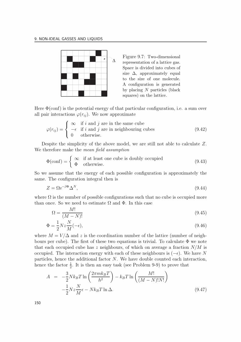
To determine the configuration integral Z we divide space into M little cubes ofvolume approximately equal to that of one particle. We will now write all integralsas sums over all cubes multiplied by ∆, the volume of one cube. The configurationintegral then equals a sum over a finite number of different configurations. A con-figuration is generated by placing each particle in any of the cubes, as in Figure 9.7.So:

Z =∑

conf

e−βΦ(conf)∆N . (9.41)

149


Figure 9.7: Two-dimensionalrepresentation of a lattice gas.Space is divided into cubes ofsize ∆, approximately equalto the size of one molecule.A configuration is generatedby placing N particles (blacksquares) on the lattice.

Here Φ(conf) is the potential energy of that particular configuration, i.e. a sum overall pair interactions ϕ(rij). We now approximate

ϕ(rij) =

∞ if i and j are in the same cube−ǫ if i and j are in neighbouring cubes0 otherwise.

(9.42)

Despite the simplicity of the above model, we are still not able to calculate Z.We therefore make the mean field assumption

Φ(conf) =

∞ if at least one cube is doubly occupiedΦ otherwise.

(9.43)

So we assume that the energy of each possible configuration is approximately thesame. The configuration integral then is

Z = Ωe−βΦ∆N , (9.44)

where Ω is the number of possible configurations such that no cube is occupied morethan once. So we need to estimate Ω and Φ. In this case

Ω =M !

(M −N)!(9.45)

Φ =1

2Nz

N

M(−ǫ), (9.46)

where M = V/∆ and z is the coordination number of the lattice (number of neigh-bours per cube). The first of these two equations is trivial. To calculate Φ we notethat each occupied cube has z neighbours, of which on average a fraction N/M isoccupied. The interaction energy with each of these neighbours is (−ǫ). We have Nparticles, hence the additional factor N . We have double counted each interaction,hence the factor 1

2. It is then an easy task (see Problem 9-9) to prove that

A = −3

2NkBT ln

(2πmkBT

h2

)− kBT ln

(M !

(M −N)!N !

)

−1

2Nz

N

Mǫ−NkBT ln ∆. (9.47)

150


For the pressure we then find

P = −kBT

∆ln

(1 − N

M

)− 1

2zǫ∆

N2

V 2. (9.48)

Making use of the approximation

ln(1 + x) ≈ x

1 + 12x, (9.49)

we finally find

P =kBT

∆

N/M

1 − 12N/M

− 1

2zǫ∆

N2

V 2

=nRT

V − nb− a

n2

V 2(9.50)

b =1

2NAv∆ (9.51)

a =1

2zǫ∆N2

Av. (9.52)

The lattice gas is therefore approximately equal to a van der Waals gas.

9.7 The regular mixture

We now consider a binary liquid mixture of NA molecules A and NB molecules B.The partition function now is

Q =

(2πmAkBT

h2

)3NA/2 (2πmBkBT

h2

)3NB/21

NA!NB!ZNA,NB

. (9.53)

Note that we need to account for indistinguishability of A and B particles separately,hence the factor 1/(NA!NB!). To calculate the configuration integral ZNA,NB

, againwe will use a lattice approach. We let the molecules A and B be of the same volume∆, and divide space in N = NA + NB = V/∆ cubes, see Figure 9.8. Note that,contrary to the lattice gas of the previous section, we now assume that all latticesites are occupied, which represents the relative incompressibility of a liquid. Theconfiguration integral now is

ZNA,NB=

∑

conf

e−βΦNA,NB(conf)∆NA+NB . (9.54)

Here ΦNA,NB(conf) is the potential energy of the given configuration. This is a sum

of all pair interactions, each approximated as

ϕ(rij) =

∞ if i and j are in the same cube−ǫij if i and j are in neighbouring cubes0 otherwise.

(9.55)

151


Figure 9.8: Two-dimensionalrepresentation of a lattice bi-nary liquid mixture. Spaceis divided into cubes of size∆, approximately equal to thesize of each molecule. Aconfiguration is generated byplacing NA particles A (blacksquares) and NB particles B

(grey squares) on the lattice.

Note that neighbouring pairs can have an interaction energy −ǫAA, −ǫBB , or −ǫAB ,depending on the molecular species at hand. This defines our model.

We now again make the mean field assumption Eq. (9.43). The configurationintegral then becomes

ZNA,NB= ΩNA,NB

e−βΦNA,NB ∆NA+NB , (9.56)

with

ΩNA,NB= (NA +NB)! (9.57)

ΦNA,NB=

1

2NA [zxA(−ǫAA) + zxB(−ǫAB)]

+1

2NB [zxA(−ǫAB) + zxB(−ǫBB)] . (9.58)

The calculation of ΩNA,NBis trivial. To calculate ΦNA,NB

we note that each moleculeA has z neighbouring cubes of which on average zNA/N = zxA are occupied by anA molecule, with each of which the interaction energy is (−ǫAA); with the otherzNB/N = zxB neighbours the interaction energy is (−ǫAB) each. The same argu-ments apply to theB molecules. In the end, we have double counted each interaction,hence the factors 1

2. For the free energy we find (Problem 9-10)

ANA,NB= −3

2NAkBT ln

(2πmAkBT

h2

)−NAkBT ln ∆

−3

2NBkBT ln

(2πmBkBT

h2

)−NBkBT ln ∆

−kBT ln

((NA +NB)!

NA!NB!

)+ ΦNA,NB

. (9.59)

In principle all thermodynamic properties can be calculated now.To connect to usual practice in thermodynamics, we will rewrite Eq. (9.59) a

little more. First we note that for NB = 0 we have

ANA= −3

2NAkBT ln

(2πmAkBT

h2

)−NAkBT ln ∆ + ΦNA

. (9.60)

152


An analogous expression can be written down for NA = 0. We therefore write

ANA,NB= ANA

+ ANB+ ∆Amix (9.61)

∆Amix = NAkBT ln xA +NBkBT ln xB + ΦNA,NB− ΦNA

− ΦNB . (9.62)

∆Amix is called the free energy of mixing. We can further simplify the energeticcontribution:

ΦNA,NB− ΦNA

− ΦNB

=1

2NA [zxA(−ǫAA) + zxB(−ǫAB)] +

1

2NB [zxA(−ǫAB) + zxB(−ǫBB)]

−1

2NAz(−ǫAA) − 1

2NBz(−ǫBB)

= (NA +NB)1

2z [xAxA(−ǫAA) − xA(−ǫAA)

+xBxB(−ǫBB) − xB(−ǫBB) + xAxB(−ǫAB − ǫAB)]

= (NA +NB)xAxB1

2z [ǫAA + ǫBB − 2ǫAB]

≡ (NA +NB)xAxBa. (9.63)

So the free energy of mixing is given by

∆Amix = NAkBT ln xA +NBkBT ln xB + (NA +NB)xAxBa. (9.64)

The chemical potential per mole of component A then becomes

µA = NAv

(∂A

∂NA

)

T,NB

= µpureA +RT ln xA + (1 − xA)2NAva, (9.65)

where µpureA is the molar chemical potential for a liquid of pure A. Note that when

the interactions between A and B are symmetrical, meaning ǫAA = ǫAB = ǫBB, wehave a = 0. In that case we speak of an ideal liquid. This expression for the chemicalpotential of an ideal liquid was used in section 4.2.3.

In Problem 9-11 we will consider the case where molecule B is larger thanmolecule A.

153


Problems

9-1. Van der Waals fluid. Experimentally, the second virial coefficient of CH4 isfound to be equal to

B2

vc= 0.430 − 0.886

Tc

T− 0.694

(Tc

T

)2

(9.66)

where Tc = 190.6 K and vc = 99.2 cm3mol−1. Describe the intermolecular interac-tion with a square-well potentiel, i.e. with potential energy ∞ for r < σ, −ǫ forσ ≤ r ≤ λσ, and 0 for r > λσ. Use the parameters ǫ/kB = 142.5 K, σ = 0.3355 nmand λ = 1.60. Calculate the experimental and theoretical values of B2 for a fewtemperatures between 100 K and 300 K.

9-2. Star polymers. A star polymer consists of f polymer “arms”, each boundwith one end to a central point. This causes the density of polymers near the centralpoint to be much higher than further away. If we dissolve many star polymers ina solvent, the polymer chains will cause an effective repulsion between the differentstar polymer centres. The closer the centres are, the larger the repulsion.

It is possible to derive the effective interaction between the central points. Theoutcome of such a calculation (we will not present the details here), in the limit ofa large number of arms f , is that the effective potential energy between two centralpoints at distance r is given by:

φ(r) = − 5

18kBTf

3/2 ln( rσ

)(r ≤ σ)

and φ(r) = 0 for r > σ. Here σ is the average diameter of the star polymer particle.We will use the virial equation here to calculate the osmotic pressure Π. At not

too high densities of star polymers, we may approximate

Π =NkBT

V

(1 +B2

n

V

)

B2 =1

2NAv

∫d3r

(1 − exp

−φ(r)

kBT

)

where n = N/NAv is the number of moles of star polymer particles.

a Plot the effective interaction versus distance r.

b Calculate the second virial coefficient B2 of star-polymers. What is the limitfor f → ∞? With what other system does this limit correspond?

c Give an expression for the osmotic pressure Π of the star polymers as a functionof the number of arms f , the particle density N/V , and temperature T .

154


9-3. Carnahan and Starling’s equation. Prove the last step in Eq. (9.13).

9-4. Carnahan and Starling’s equation (2). Show that Eq. (9.13) follows fromEq. (9.14).

9-5. Free energy of a Van der Waals fluid. Derive Eq. (9.18) from Eq. (9.17).

9-6. Parameters of the Van der Waals fluid. The parameters of the Van derWaals equation of state can be calculated from knowledge of the critical temperatureand pressure:

a =27

64

R2T 2c

Pcb =

RTc

8Pc

Using this, show that for a Lennard-Jones potential follows

ǫ

k=

81

64Tc

ǫ

σ3=

27

4πPc

With this result, calculate ǫ/k and σ for the molecules Ar, CH4, N2 and CO2. Given:Ar: Tc = 150.9 K, Pc = 48.98 bar;N2: Tc = 126.1 K, Pc = 33.94 bar;CH4: Tc = 190.6 K, Pc = 46.04 bar;CO2: Tc = 304.2 K, Pc = 73.82 bar.Compare your answers with the following experimental values, which have been fitto second virial coefficients:Ar: ǫ/kB = 177.7 K, σ = 0.3504 nm;N2: ǫ/kB = 95.2 K, σ = 0.3745 nm;CH4: ǫ/kB = 148.9 K, σ = 0.3783 nm;CO2: ǫ/kB = 198.2 K, σ = 0.4328 nm.From computer simulations it is found that for real Lennard-Jones fluids:

ǫ

kB= 0.722Tc

ǫ

σ3= 7.42Pc

Calculate ǫ/kB and σ for Ar, CH4, N2 and CO2 using this expression too.

9-7. Fugacity and virial equation. Calculate the fugacity coefficient of a gasobeying the virial equation.

9-8. P as power series in ρ instead of z. Check Eqs. (9.38) and (9.39).

9-9. Pressure of a lattice gas. Prove Eqs. (9.47) and (9.48).

155


9-10. Free energy of a binary mixture. Prove Eq. (9.59).

9-11. Binary mixture of large and small molecules. Consider a binary liquidmixture of NA molecules A and NB molecules B. The volumes per molecule are vA

and vB respectively, where we assume vB = pvA and p > 1 is an integer number.Both molecules are inflexible. The partition function of the system is:

Q =

(2πmAkBT

h2

)3NA/2 (2πmBkBT

h2

)3NB/21

NA!NB!ZNA,NB

ZNA,NB=

∫d3NAr

∫d3NBx exp

−βΦ(r3NA , x3NB)

.

Here Φ(r3NA, x3NB ) is the potential energy of the system if the A molecules are atpositions r1 to rNA

and the B molecules are at positions x1 to xNB. We assume that

the interactions between the molecules are merely hard repulsions, and that thereare no attractions. The number of configurations the system can have without twoor more molecules overlapping is called ΩNA,NB

. We assume that the volume of thesystem equals

V = NAvA +NBvB,

i.e. there is no unoccupied space (incompressible liquid).

(a) Give the formula for ΩNA,NB. Do this along the following route: First di-

vide the volume in cubes of size vB and place the NB molecules of kind B.Then subdivide the remaining cubes in smaller cubes of size vA and place themolecules of kind A.

(b) Again calculate ΩNA,NB, but now in the following way: Again first place the

molecules of kind B, but now in a space that has been divided in cubes of sizevA. Next place the molecules of kind A in the remaining cubes.

(c) Show that the configuration integral in case (a) may be written as

ZNA,NB= Ω

(a)NA,NB

vNA

A vNB

B ,

and in case (b) as

ZNA,NB= Ω

(b)NA,NB

vNA

A vNB

A ,

and show that both formulas give the same result.

(d) Calculate ∆Amix in

ANA,NB= ANA

+ ANB+ ∆Amix

(e) Calculate µA and µB, the molar chemical potentials of component A andcomponent B.

156

Appendix A

Useful mathematical relations andphysical constants

A.1 Gaussian integrals

We will often need to evaluate integrals of the form

In(α) =

∫∞

0

dx xne−αx2

. (A.1)

Solutions to these integrals can easily be generated by “differentiating under theintegral sign”:

In+2(α) =

∫∞

0

dx xn+2e−αx2

= − ∂

∂αIn(α). (A.2)

Knowledge of the solution for n = 0 allows us to generate solutions for all even n,whereas the solution for n = 1 allows us to generate solutions for all odd n.

Although the solution for n = 1 can easily be found, I1(α) = 1/(2α), the solutionfor n = 0 requires some more thought. It can be calculated by considering thefollowing integral in the two-dimensional plane:

∫∞

0

dx

∫∞

0

dy e−α(x2+y2). (A.3)

Because we can factorize the exponential this is clearly equal to [I0(α)]2. Changingfrom (x, y) to polar coordinates (r, φ), taking into account the Jacobian, we find

I20 (α) =

∫∞

0

dr

∫ π/2

0

dφ re−αr2

=π

4α. (A.4)

Hence I0(α) = 12

√πα.

157

A. USEFUL MATHEMATICAL RELATIONS AND PHYSICAL CONSTANTS

The integrals In appear so often that we write down the values of some of themexplicitly. We have

I0 =1

2

(πα

)1/2

, I2 =1

4

( π

α3

)1/2

, I4 =3

8

( π

α5

)1/2

, . . . (A.5)

and

I1 =1

2α, I3 =

1

2α2, I5 =

1

α3, . . . . (A.6)

A.2 Relations between partial derivatives

Suppose there is a relation between the variables x, y, and z:

F (x, y, z) = 0, (A.7)

meaning that only two of them are independent. We could rearrange this equationto give x as a function of y and z as

x = x(y, z). (A.8)

If we make infinitesimal changes dy and dz in y and z, there will be an infinitesimalchange in x according to

dx =

(∂x

∂y

)

z

dy +

(∂x

∂z

)

y

dz. (A.9)

Similarly, writing y = y(x, z),

dy =

(∂y

∂x

)

z

dx+

(∂y

∂z

)

x

dz. (A.10)

Substituting Eq. (A.10) in Eq. (A.9), we find

dx =

(∂x

∂y

)

z

(∂y

∂x

)

z

dx+

[(∂x

∂y

)

z

(∂y

∂z

)

x

+

(∂x

∂z

)

y

]dz. (A.11)

We now take x and z as the independent variables. First we choose dz = 0 and anon-zero value for dx. Dividing both sides of Eq. (A.11) by dx we find

1 =

(∂x

∂y

)

z

(∂y

∂x

)

z

, (A.12)

158


or

(∂x

∂y

)

z

=

(∂y

∂x

)−1

z

. (A.13)

Second, we choose dx = 0 and a non-zero value for dz. Dividing Eq. (A.11) by dzwe find

(∂x

∂y

)

z

(∂y

∂z

)

x

= −(∂x

∂z

)

y

, (A.14)

or

(∂x

∂y

)

z

(∂y

∂z

)

x

(∂z

∂x

)

y

= −1. (A.15)

This is sometimes called the -1 rule, or cyclical relation.Do not confuse the -1 rule with the well-known chain rule of differentiation. A

derivation of the chain rule goes as follows. Suppose again that x, y and z are notindependent, being related by F (x, y, z) = 0. Let us consider some other functionG of x, y and z. Because x, y and z are interrelated, G may be expressed in termsof only two of the variables, say

G = G(x, y). (A.16)

This can be rearranged to give

x = x(G, y), (A.17)

so

dx =

(∂x

∂G

)

y

dG+

(∂x

∂y

)

G

dy. (A.18)

Dividing both sides by dz, holding G constant, we find the chain rule:

(∂x

∂z

)

G

=

(∂x

∂y

)

G

(∂y

∂z

)

G

. (A.19)

Note the common G outside each partial differential.Other relations may be constructed when needed. For example, suppose again

that x, y and z are not independent. We again may write x = x(y, z) and form adifferential for x:

dx =

(∂x

∂y

)

z

dy +

(∂x

∂z

)

y

dz. (A.20)

159


Let us consider some other function H , also of y and z. The derivative of x withrespect to z at constant H (not to be confused with the partial derivative of x withrespect to z at constant y) can be found by dividing both sides by dz, holding Hconstant:

(∂x

∂z

)

H

=

(∂x

∂y

)

z

(∂y

∂z

)

H

+

(∂x

∂z

)

y

. (A.21)

A.3 Geometric series

The geometric series Sn(x) is defined as

Sn(x) =n∑

k=0

xn = 1 + x+ x2 + . . .+ xn. (A.22)

Multiplying both sides by x we find

xSn(x) = x+ x2 + x3 + . . .+ xn+1. (A.23)

Subtracting these two equations yields

(1 − x)Sn(x) = 1 − xn+1. (A.24)

So we find

n∑

k=0

xn =1 − xn+1

1 − x. (A.25)

For −1 < x < 1 the series converges as n→ ∞, in which case

∞∑

k=0

xn =1

1 − x(|x| < 1). (A.26)

A.4 Taylor series

A Taylor series is a series expansion of a function around a certain point. In onedimension, the Taylor series of a function f around the point x = a is given by

f(x) = f(a)+f ′(a)(x−a)+1

2f ′′(a)(x−a)2+

1

6f ′′′(a)(x−a)3+. . .+

1

n!f (n)(a)(x−a)n+. . . ,

(A.27)

160


where f (n)(a) denotes the n-th derivative of f at x = a.Here follow a few examples:

exp(x) = 1 + x+1

2x2 +

1

6x3 + . . .+

1

n!xn + . . . (A.28)

ln(1 + x) = x− 1

2x2 +

1

3x3 + . . .+

(−1)n−1

nxn + . . . (A.29)

cos(x) = 1 − 1

2x2 +

1

24x4 + . . .+

cos(nπ/2)

n!xn + . . . (A.30)

sin(x) = x− 1

6x3 +

1

120x5 + . . .+

sin(nπ/2)

n!xn + . . . (A.31)

A.5 Logarithms and exponentials

When manipulating logarithms and exponentials remember the following rules:

exp(a+ b) = exp(a) exp(b) (A.32)

exp(a ln b) = ba (A.33)

exp(ab) = (exp(a))b = (exp(b))a (A.34)

ln(ab) = ln(a) + ln(b) (A.35)

ln(ba) = a ln(b) (A.36)

Derivatives are given by

d

dxb exp(ax) = ab exp(ax) (A.37)

d

dxax = ln(a) ax (A.38)

d

dxb ln(cxa) = b

a

x(A.39)

and integrals by∫

exp(ax)dx =1

aexp(ax) (A.40)

∫ln(ax)dx = x ln(ax) − x (A.41)

161


A.6 Physical constants

Planck’s constant, h = 6.62607 × 10−34 J satomic mass unit, u = 1.66054 × 10−27 kgBoltzmann’s constant, kB = 1.38065× 10−23 J/KAvogadro’s number, NAv = 6.02214 × 1023 mol−1

Universal gas constant, R = 8.3145 J/K mol−1

Speed of light, c = 2.99792 × 108 m/s

162

chapter 8 interacting systems

Documents