Chapter 8

Non-likelihood methods

8.1 Loss functions

Up until now our main focus has been on parameter estimating via the maximum likeli-

hood. However, the negative maximum likelihood is simply one member of loss criterions.

Loss functions are usually distances, such as the `1 and `2 distance. Typically we estimate

a parameter by minimising the loss function, and using as the estimator the parameter

which minimises the loss. Usually (but not always) the way to solve the loss function is

to di↵erentiate it and equate it to zero. Below we give examples of loss functions whose

formal derivative does not exist.

8.1.1 L1-loss functions

The Laplacian

Consider the Laplacian (also known as the double exponential), which is defined as

f(y; ✓, ⇢) =1

2⇢exp

✓

� |y � ✓|⇢

◆

=

8

<

:

12⇢exp

⇣

y�✓⇢

⌘

y < ✓

12⇢exp

⇣

✓�y⇢

⌘

y � ✓.

We observe {Yi} and our objective is to estimate the location parameter ✓, for now the

scale parameter ⇢ is not of interest. The log-likelihood is

Ln(✓, ⇢) = �n log 2⇢� ⇢�1 1

2

nX

i=1

|Yi � ✓|| {z }

=Ln

(✓)

.

223

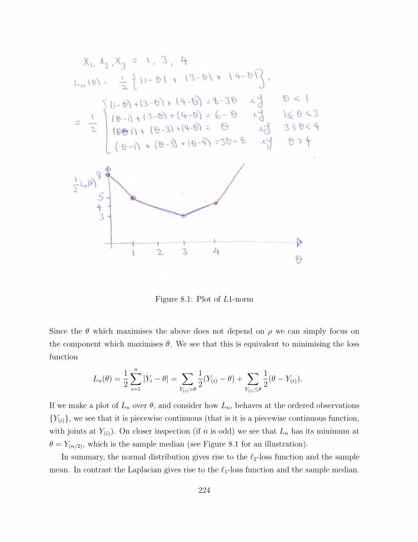
Figure 8.1: Plot of L1-norm

Since the ✓ which maximises the above does not depend on ⇢ we can simply focus on

the component which maximises ✓. We see that this is equivalent to minimising the loss

function

Ln(✓) =1

2

nX

i=1

|Yi � ✓| =X

Y(i)>✓

1

2(Y(i) � ✓) +

X

Y(i)✓

1

2(✓ � Y(i)).

If we make a plot of Ln over ✓, and consider how Ln, behaves at the ordered observations

{Y(i)}, we see that it is piecewise continuous (that is it is a piecewise continuous function,

with joints at Y(i)). On closer inspection (if n is odd) we see that Ln has its minimum at

✓ = Y(n/2), which is the sample median (see Figure 8.1 for an illustration).

In summary, the normal distribution gives rise to the `2-loss function and the sample

mean. In contrast the Laplacian gives rise to the `1-loss function and the sample median.

224

The asymmetric Laplacian

Consider the generalisation of the Laplacian, usually called the assymmetric Laplacian,

which is defined as

f(y; ✓, ⇢) =

8

<

:

p⇢exp

⇣

py�✓⇢

⌘

y < ✓(1�p)

⇢exp

⇣

�(1� p)y�✓⇢

⌘

y � ✓.

where 0 < p < 1. The corresponding negative likelihood to estimate ✓ is

Ln(✓) =X

Y(i)>✓

(1� p)(Yi � ✓) +X

Y(i)✓

p(✓ � Yi).

Using similar arguments to those in part (i), it can be shown that the minimum of Ln is

approximately the pth quantile.

8.2 Estimating Functions

8.2.1 Motivation

Estimating functions are a unification and generalisation of the maximum likelihood meth-

ods and the method of moments. It should be noted that it is a close cousin of the gen-

eralised method of moments and generalised estimating equation. We first consider a few

examples and will later describe a feature common to all these examples.

Example 8.2.1 (i) Let us suppose that {Yi} are iid random variables with Yi ⇠ N (µ, �2).

The log-likelihood in proportional to

Ln(µ, �2) = �1

2log �2 � 1

2�2

nX

i=1

(Xi � µ)2.

We know that to estimate µ and �2 we use the µ and �2 which are the solution of

�1

2�2+

1

2�4

nX

i=1

(Xi � µ)2 = 01

�2

nX

i=1

(Xi � µ) = 0. (8.1)

(ii) In general suppose {Yi} are iid random variables with Yi ⇠ f(·; ✓). The log-likelihoodis Ln(✓) =

Pni=1 log f(✓;Yi). If the regularity conditions are satisfied then to esti-

mate ✓ we use the solution of

@Ln(✓)

@✓= 0. (8.2)

225

(iii) Let us suppose that {Xi} are iid random variables with a Weibull distribution f(x; ✓) =

(↵�)(x

�)↵ exp(�(x/�)↵), where ↵,� > 0.

We know that E(X) = ��(1+↵�1) and E(X2) = �2�(1+2↵�1). Therefore E(X)���(1 + ↵�1) = 0 and E(X2)� �2�(1 + 2↵�1) = 0. Hence by solving

1

n

nX

i=1

Xi � ��(1 + ↵�1) = 01

n

nX

i=1

X2i � �2�(1 + 2↵�1) = 0, (8.3)

we obtain estimators of ↵ and �. This is essentially a method of moments estimator

of the parameters in a Weibull distribution.

(iv) We can generalise the above. It can be shown that E(Xr) = �r�(1 + r↵�1). There-

fore, for any distinct s and r we can estimate ↵ and � using the solution of

1

n

nX

i=1

Xri � �r�(1 + r↵�1) = 0

1

n

nX

i=1

Xsi � �s�(1 + s↵�1) = 0. (8.4)

(v) Consider the simple linear regression Yi = ↵xi + "i, with E("i) = 0 and var("i) = 1,

the least squares estimator of ↵ is the solution of

1

n

nX

i=1

(Yi � axi)xi = 0. (8.5)

We observe that all the above estimators can be written as the solution of a homoge-

nous equations - see equations (8.1), (8.2), (8.3), (8.4) and (8.5). In other words, for

each case we can define a random function Gn(✓), such that the above estimators are the

solutions of Gn(✓n) = 0. In the case that {Yi} are iid then Gn(✓) =Pn

i=1 g(Yi; ✓), for some

function g(Yi; ✓). The function Gn(✓) is called an estimating function. All the function

Gn, defined above, satisfy the unbiased property which we define below.

Definition 8.2.1 (Estimating function) An estimating function Gn is called unbiased

if at the true parameter ✓0 Gn(·) satisfies

E [Gn(✓0)] = 0.

If there are p unknown parameters and p estimating equations, the estimation equation

estimator is the ✓ which solves Gn(✓) = 0.

226

Hence the estimating function is an alternative way of viewing parameter estimating.

Until now, parameter estimators have been defined in terms of the maximum of the

likelihood. However, an alternative method for defining an estimator is as the solution

of a function. For example, suppose that {Yi} are random variables, whose distribution

depends in some way on the parameter ✓0. We want to estimate ✓0, and we know that

there exists a function such that G(✓0) = 0. Therefore using the data {Yi} we can define

a random function, Gn where E(Gn(✓)) = G(✓) and use the parameter ✓n, which satisfies

Gn(✓) = 0, as an estimator of ✓. We observe that such estimators include most maximum

likelihood estimators and method of moment estimators.

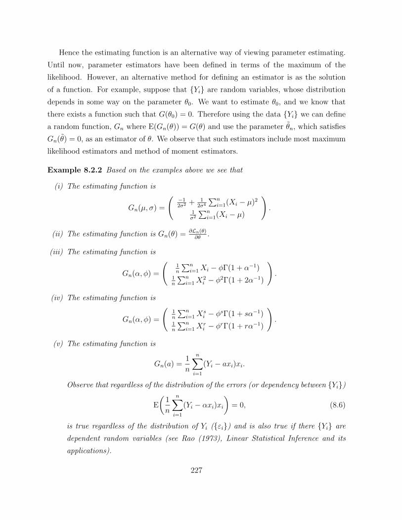
Example 8.2.2 Based on the examples above we see that

(i) The estimating function is

Gn(µ, �) =

�12�2 +

12�4

Pni=1(Xi � µ)2

1�2

Pni=1(Xi � µ)

!

.

(ii) The estimating function is Gn(✓) =@L

n

(✓)@✓

.

(iii) The estimating function is

Gn(↵,�) =

1n

Pni=1 Xi � ��(1 + ↵�1)

1n

Pni=1 X

2i � �2�(1 + 2↵�1)

!

.

(iv) The estimating function is

Gn(↵,�) =

1n

Pni=1 X

si � �s�(1 + s↵�1)

1n

Pni=1 X

ri � �r�(1 + r↵�1)

!

.

(v) The estimating function is

Gn(a) =1

n

nX

i=1

(Yi � axi)xi.

Observe that regardless of the distribution of the errors (or dependency between {Yi})

E

✓

1

n

nX

i=1

(Yi � ↵xi)xi

◆

= 0, (8.6)

is true regardless of the distribution of Yi ({"i}) and is also true if there {Yi} are

dependent random variables (see Rao (1973), Linear Statistical Inference and its

applications).

227

The advantage of this approach is that sometimes the solution of an estimating equa-

tion will have a smaller finite sample variance than the MLE. Even though asymptotically

(under certain conditions) the MLE will asymptotically attain the Cramer-Rao bound

(which is the smallest variance). Moreover, MLE estimators are based on the assump-

tion that the distribution is known (else the estimator is misspecified - see Section 5.1.1),

however sometimes an estimating equation can be free of such assumptions.

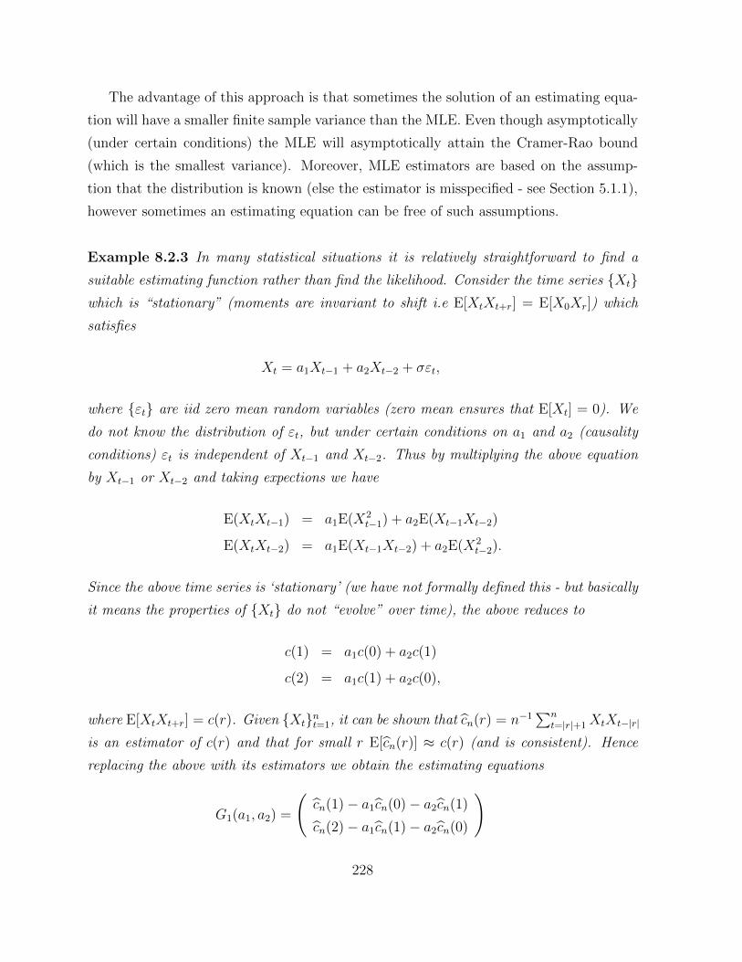
Example 8.2.3 In many statistical situations it is relatively straightforward to find a

suitable estimating function rather than find the likelihood. Consider the time series {Xt}which is “stationary” (moments are invariant to shift i.e E[XtXt+r] = E[X0Xr]) which

satisfies

Xt = a1Xt�1 + a2Xt�2 + �"t,

where {"t} are iid zero mean random variables (zero mean ensures that E[Xt] = 0). We

do not know the distribution of "t, but under certain conditions on a1 and a2 (causality

conditions) "t is independent of Xt�1 and Xt�2. Thus by multiplying the above equation

by Xt�1 or Xt�2 and taking expections we have

E(XtXt�1) = a1E(X2t�1) + a2E(Xt�1Xt�2)

E(XtXt�2) = a1E(Xt�1Xt�2) + a2E(X2t�2).

Since the above time series is ‘stationary’ (we have not formally defined this - but basically

it means the properties of {Xt} do not “evolve” over time), the above reduces to

c(1) = a1c(0) + a2c(1)

c(2) = a1c(1) + a2c(0),

where E[XtXt+r] = c(r). Given {Xt}nt=1, it can be shown that bcn(r) = n�1Pn

t=|r|+1 XtXt�|r|

is an estimator of c(r) and that for small r E[bcn(r)] ⇡ c(r) (and is consistent). Hence

replacing the above with its estimators we obtain the estimating equations

G1(a1, a2) =

bcn(1)� a1bcn(0)� a2bcn(1)

bcn(2)� a1bcn(1)� a2bcn(0)

!

228

8.2.2 The sampling properties

We now show that under certain conditions ✓n is a consistent estimator of ✓.

Theorem 8.2.1 Suppose that Gn(✓) is an unbiased estimating function, where Gn(✓n) =

0 and E(Gn(✓0)) = 0.

(i) If ✓ is a scalar, for every n Gn(✓) is a continuous monotonically decreasing function

in ✓ and for all ✓ Gn(✓)P! E(Gn(✓)) (notice that we do require an equicontinuous

assumption), then we have ✓nP! ✓0.

(ii) If we can show that sup✓ |Gn(✓) � E(Gn(✓))|P! 0 and E(Gn(✓)) is uniquely zero at

✓0 then we have ✓nP! ✓0.

PROOF. The proof of case (i) is relatively straightforward (see also page 318 in Davison

(2002)). The idea is to exploit the monotonicity property of Gn(·) to show for every

" > 0 P (e✓n < ✓0 � " or e✓n > ✓0 + ") ! 0 as n ! 1. The proof is best understand by

making a plot of Gn(✓) with ✓n < ✓0 � " < ✓0 (see Figure 8.2). We first note that since

E[Gn(✓0)] = 0, then for any fixed " > 0

Gn(✓0 � ")P! E

⇥

Gn(✓0 � ")⇤

> 0, (8.7)

since Gn is monotonically decreasing for all n. Now, since Gn(✓) is monotonically de-

creasing we see that ✓n < (✓0 � ") implies Gn(✓n) � Gn(✓0 � ") > 0 (and visa-versa)

hence

P�

✓n � (✓0 � ") 0�

= P�

Gn(✓n)�Gn(✓0 � ") > 0�

.

But we have from (8.7) that E(Gn(✓0 � "))P! E(Gn(✓0 � ")) > 0. Thus P

�

Gn(✓n) �Gn(✓0 � ") > 0

� P! 0 and

P�

✓n � (✓0 � ") < 0� P! 0 as n ! 1.

A similar argument can be used to show that that P�

✓n � (✓0 + ") > 0� P! 0 as n ! 1.

As the above is true for all ", together they imply that ✓nP! ✓0 as n ! 1.

The proof of (ii) is more involved, but essentially follows the lines of the proof of

Theorem 2.6.1. ⇤

We now show normality, which will give us the variance of the limiting distribution ofe✓n.

229

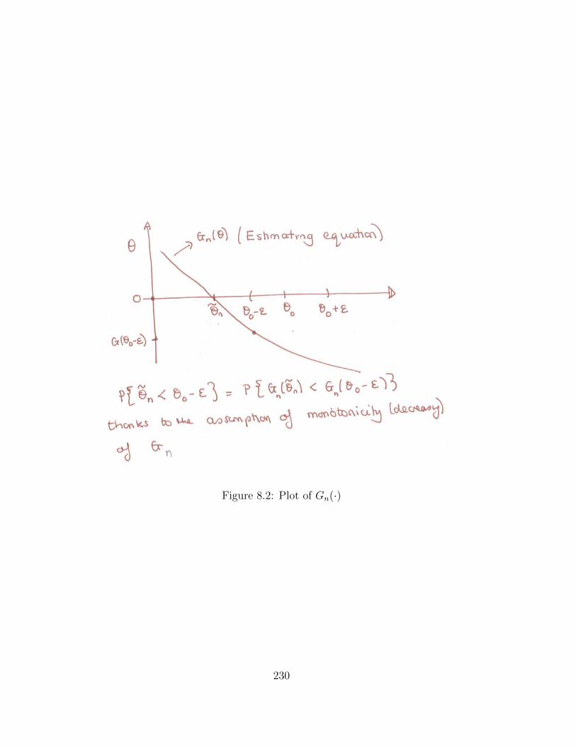
Figure 8.2: Plot of Gn(·)

230

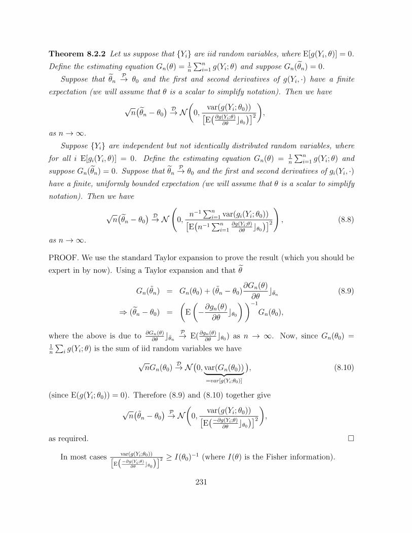
Theorem 8.2.2 Let us suppose that {Yi} are iid random variables, where E[g(Yi, ✓)] = 0.

Define the estimating equation Gn(✓) =1n

Pni=1 g(Yi; ✓) and suppose Gn(e✓n) = 0.

Suppose that e✓nP! ✓0 and the first and second derivatives of g(Yi, ·) have a finite

expectation (we will assume that ✓ is a scalar to simplify notation). Then we have

pn�

e✓n � ✓0� D! N

✓

0,var(g(Yi; ✓0))⇥

E�@g(Y

i

;✓)@✓

c✓0�⇤2

◆

,

as n ! 1.

Suppose {Yi} are independent but not identically distributed random variables, where

for all i E[gi(Yi, ✓)] = 0. Define the estimating equation Gn(✓) = 1n

Pni=1 g(Yi; ✓) and

suppose Gn(e✓n) = 0. Suppose that e✓nP! ✓0 and the first and second derivatives of gi(Yi, ·)

have a finite, uniformly bounded expectation (we will assume that ✓ is a scalar to simplify

notation). Then we have

pn�

e✓n � ✓0� D! N

0,n�1

Pni=1 var(gi(Yi; ✓0))

⇥

E�

n�1Pn

i=1@g(Y

i

;✓)@✓

c✓0�⇤2

!

, (8.8)

as n ! 1.

PROOF. We use the standard Taylor expansion to prove the result (which you should be

expert in by now). Using a Taylor expansion and that e✓

Gn(✓n) = Gn(✓0) + (✓n � ✓0)@Gn(✓)

@✓c✓

n

(8.9)

) (e✓n � ✓0) =

✓

E

✓

�@gn(✓)

@✓c✓0◆◆�1

Gn(✓0),

where the above is due to @Gn

(✓)@✓

c✓n

P! E(@gn(✓)@✓

c✓0) as n ! 1. Now, since Gn(✓0) =1n

P

i g(Yi; ✓) is the sum of iid random variables we have

pnGn(✓0)

D! N�

0, var(Gn(✓0))| {z }

=var[g(Yi

;✓0)]

�

, (8.10)

(since E(g(Yi; ✓0)) = 0). Therefore (8.9) and (8.10) together give

pn�

✓n � ✓0� P! N

✓

0,var(g(Yi; ✓0))

⇥

E��@g(Y

i

;✓)@✓

c✓0�⇤2

◆

,

as required. ⇤

In most cases var(g(Yi

;✓0))⇥

E�

�@g(Yi

;✓)@✓

c✓0

�⇤2 � I(✓0)�1 (where I(✓) is the Fisher information).

231

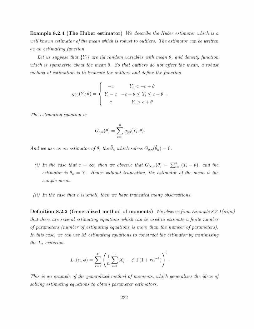
Example 8.2.4 (The Huber estimator) We describe the Huber estimator which is a

well known estimator of the mean which is robust to outliers. The estimator can be written

as an estimating function.

Let us suppose that {Yi} are iid random variables with mean ✓, and density function

which is symmetric about the mean ✓. So that outliers do not e↵ect the mean, a robust

method of estimation is to truncate the outliers and define the function

g(c)(Yi; ✓) =

8

>

>

<

>

>

:

�c Yi < �c+ ✓

Yi � c �c+ ✓ Yi c+ ✓

c Yi > c+ ✓

.

The estimating equation is

Gc,n(✓) =nX

i=1

g(c)(Yi; ✓).

And we use as an estimator of ✓, the ✓n which solves Gc,n(✓n) = 0.

(i) In the case that c = 1, then we observe that G1,n(✓) =Pn

i=1(Yi � ✓), and the

estimator is ✓n = Y . Hence without truncation, the estimator of the mean is the

sample mean.

(ii) In the case that c is small, then we have truncated many observations.

Definition 8.2.2 (Generalized method of moments) We observe from Example 8.2.1(iii,iv)

that there are several estimating equations which can be used to estimate a finite number

of parameters (number of estimating equations is more than the number of parameters).

In this case, we can use M estimating equations to construct the estimator by minimising

the L2 criterion

Ln(↵,�) =MX

r=1

1

n

nX

i=1

Xri � �r�(1 + r↵�1)

!2

.

This is an example of the generalized method of moments, which generalizes the ideas of

solving estimating equations to obtain parameter estimators.

232

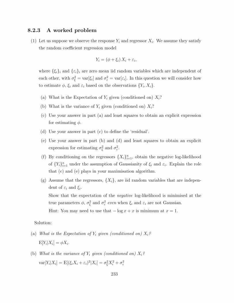
8.2.3 A worked problem

(1) Let us suppose we observe the response Yi and regressor Xi. We assume they satisfy

the random coe�cient regression model

Yi = (�+ ⇠i)Xi + "i,

where {⇠i}i and {"i}i are zero mean iid random variables which are independent of

each other, with �2⇠ = var[⇠i] and �2

" = var["i]. In this question we will consider how

to estimate �, ⇠i and "i based on the observations {Yi, Xi}.

(a) What is the Expectation of Yi given (conditioned on) Xi?

(b) What is the variance of Yi given (conditioned on) Xi?

(c) Use your answer in part (a) and least squares to obtain an explicit expression

for estimating �.

(d) Use your answer in part (c) to define the ‘residual’.

(e) Use your answer in part (b) and (d) and least squares to obtain an explicit

expression for estimating �2⇠ and �2

" .

(f) By conditioning on the regressors {Xi}ni=1, obtain the negative log-likelihood

of {Yi}ni=1 under the assumption of Gaussianity of ⇠i and "i. Explain the role

that (c) and (e) plays in your maximisation algorithm.

(g) Assume that the regressors, {Xi}, are iid random variables that are indepen-

dent of "i and ⇠i.

Show that the expectation of the negative log-likelihood is minimised at the

true parameters �, �2⇠ and �2

" even when ⇠i and "i are not Gaussian.

Hint: You may need to use that � log x+ x is minimum at x = 1.

Solution:

(a) What is the Expectation of Yi given (conditioned on) Xi?

E[Yi|Xi] = �Xi.

(b) What is the variance of Yi given (conditioned on) Xi?

var[Yi|Xi] = E[(⇠iXi + "i)2|Xi] = �2⇠X

2i + �2

"

233

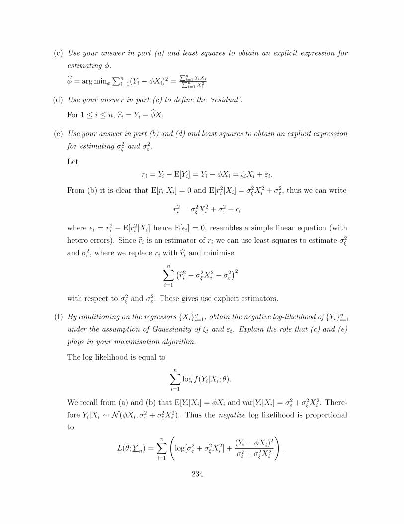
(c) Use your answer in part (a) and least squares to obtain an explicit expression for

estimating �.

b� = argmin�

Pni=1(Yi � �Xi)2 =

Pn

i=1 Yi

XiP

n

i=1 X2i

(d) Use your answer in part (c) to define the ‘residual’.

For 1 i n, bri = Yi � b�Xi

(e) Use your answer in part (b) and (d) and least squares to obtain an explicit expression

for estimating �2⇠ and �2

" .

Let

ri = Yi � E[Yi] = Yi � �Xi = ⇠iXi + "i.

From (b) it is clear that E[ri|Xi] = 0 and E[r2i |Xi] = �2⇠X

2i + �2

" , thus we can write

r2i = �2⇠X

2i + �2

" + ✏i

where ✏i = r2i � E[r2i |Xi] hence E[✏i] = 0, resembles a simple linear equation (with

hetero errors). Since bri is an estimator of ri we can use least squares to estimate �2⇠

and �2" , where we replace ri with bri and minimise

nX

i=1

�

br2i � �2⇠X

2i � �2

"

�2

with respect to �2⇠ and �2

" . These gives use explicit estimators.

(f) By conditioning on the regressors {Xi}ni=1, obtain the negative log-likelihood of {Yi}ni=1

under the assumption of Gaussianity of ⇠t and "t. Explain the role that (c) and (e)

plays in your maximisation algorithm.

The log-likelihood is equal to

nX

i=1

log f(Yi|Xi; ✓).

We recall from (a) and (b) that E[Yi|Xi] = �Xi and var[Yi|Xi] = �2" +�2

⇠X2i . There-

fore Yi|Xi ⇠ N (�Xi, �2" + �2

⇠X2i ). Thus the negative log likelihood is proportional

to

L(✓;Y n) =nX

i=1

log[�2" + �2

⇠X2i ] +

(Yi � �Xi)2

�2" + �2

⇠X2i

!

.

234

We choose the parameters which minimise L(✓;Y n). We note that this means we

need to take the derivative of L(✓;Y n) with respect to the three parameters and

solve using the Newton Raphson scheme. However, the estimators obtained in (c)

and (d) can be used as initial values in the scheme.

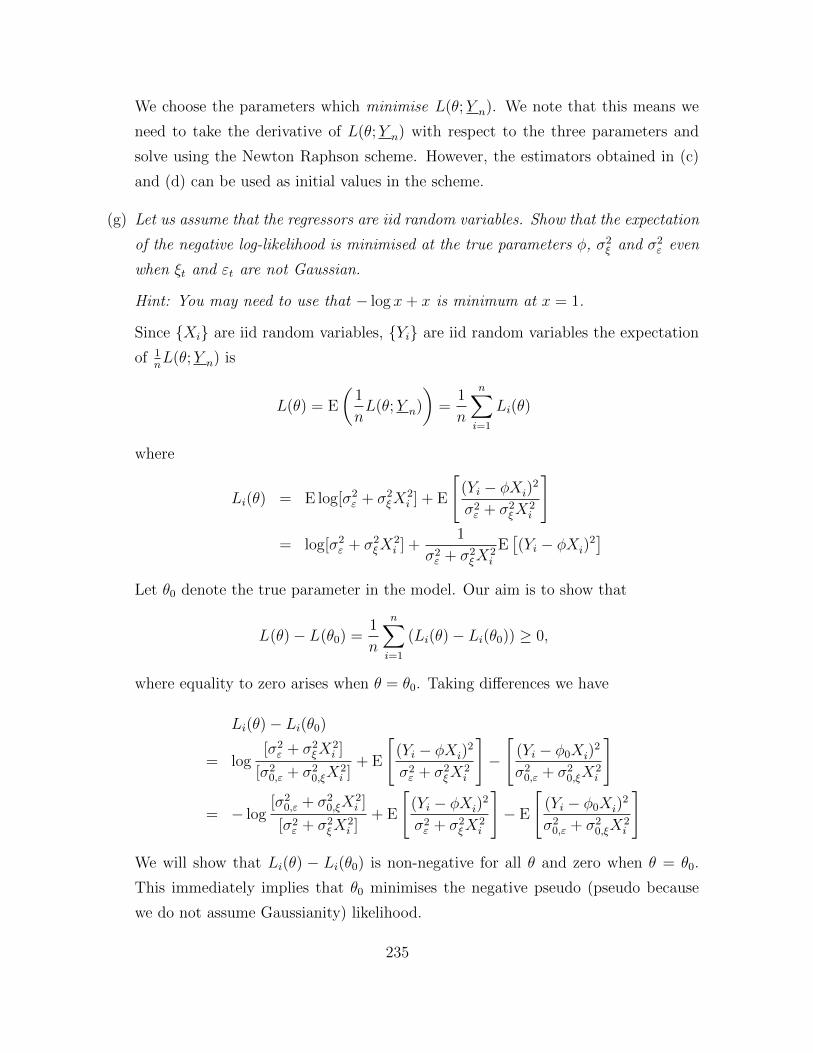
(g) Let us assume that the regressors are iid random variables. Show that the expectation

of the negative log-likelihood is minimised at the true parameters �, �2⇠ and �2

" even

when ⇠t and "t are not Gaussian.

Hint: You may need to use that � log x+ x is minimum at x = 1.

Since {Xi} are iid random variables, {Yi} are iid random variables the expectation

of 1nL(✓;Y n) is

L(✓) = E

✓

1

nL(✓;Y n)

◆

=1

n

nX

i=1

Li(✓)

where

Li(✓) = E log[�2" + �2

⇠X2i ] + E

"

(Yi � �Xi)2

�2" + �2

⇠X2i

#

= log[�2" + �2

⇠X2i ] +

1

�2" + �2

⇠X2i

E⇥

(Yi � �Xi)2⇤

Let ✓0 denote the true parameter in the model. Our aim is to show that

L(✓)� L(✓0) =1

n

nX

i=1

(Li(✓)� Li(✓0)) � 0,

where equality to zero arises when ✓ = ✓0. Taking di↵erences we have

Li(✓)� Li(✓0)

= log[�2

" + �2⇠X

2i ]

[�20," + �2

0,⇠X2i ]

+ E

"

(Yi � �Xi)2

�2" + �2

⇠X2i

#

�"

(Yi � �0Xi)2

�20," + �2

0,⇠X2i

#

= � log[�2

0," + �20,⇠X

2i ]

[�2" + �2

⇠X2i ]

+ E

"

(Yi � �Xi)2

�2" + �2

⇠X2i

#

� E

"

(Yi � �0Xi)2

�20," + �2

0,⇠X2i

#

We will show that Li(✓) � Li(✓0) is non-negative for all ✓ and zero when ✓ = ✓0.

This immediately implies that ✓0 minimises the negative pseudo (pseudo because

we do not assume Gaussianity) likelihood.

235

Our aim is to place the di↵erence in the form �logx+ x plus an additional positive

term (it is similar in idea to completing the square), but requires a lot of algebraic

manipulation. Let

Li(✓)� Li(✓0) = Ai(✓) + Bi(✓)

where

Ai(✓) = �

log[�2

0," + �20,⇠X

2i ]

[�2" + �2

⇠X2i ]

!

Bi(✓) = E

"

(Yi � �Xi)2

�2" + �2

⇠X2i

#

� E

"

(Yi � �0Xi)2

�20," + �2

0,⇠X2i

#

.

First consider the di↵erence

Bi(✓) = E

"

(Yi � �Xi)2

�2" + �2

⇠X2i

#

� E

"

(Yi � �0Xi)2

�20," + �2

0,⇠X2i

#

| {z }

=(�20,"+�2

0,⇠X2i

)�1var(Yi

)=1

= E

"

(Yi � �Xi)2

�2" + �2

⇠X2i

#

� 1.

Now replace � by �0

Bi(✓) = E

"

(Yi � �0Xi)2

�2" + �2

⇠X2i

#

+ E

"

(Yi � �Xi)2 � (Yi � �0Xi)

2

�2" + �2

⇠X2i

#

� 1

= E

"

("t + ⇠iXi)2

�2" + �2

⇠X2i

#

+ E

"

2(�� �0)(Yi � �0Xi)Xi

�2" + �2

⇠X2i

#

+

E

"

(�� �0)2X2i

�2" + �2

⇠X2i

#

� 1

=E [("t + ⇠iXi)2]

�2" + �2

⇠X2i

+ E

"

2(�� �0)(Yi � �0Xi)Xi

�2" + �2

⇠X2i

#

+

(�� �0)2X2i

�2" + �2

⇠X2i

� 1

=�20," + �2

0,⇠X2i

�2" + �2

⇠X2i

+(�� �0)2X2

i

�2" + �2

⇠X2i

� 1.

236

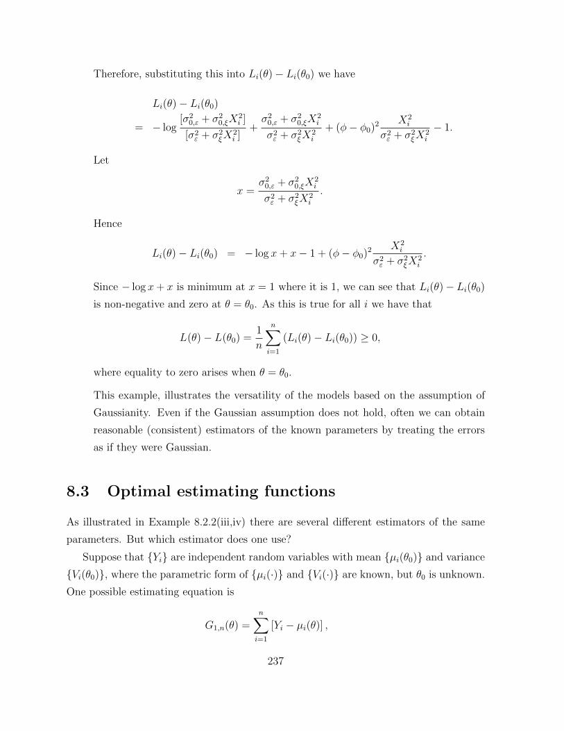
Therefore, substituting this into Li(✓)� Li(✓0) we have

Li(✓)� Li(✓0)

= � log[�2

0," + �20,⇠X

2i ]

[�2" + �2

⇠X2i ]

+�20," + �2

0,⇠X2i

�2" + �2

⇠X2i

+ (�� �0)2 X2

i

�2" + �2

⇠X2i

� 1.

Let

x =�20," + �2

0,⇠X2i

�2" + �2

⇠X2i

.

Hence

Li(✓)� Li(✓0) = � log x+ x� 1 + (�� �0)2 X2

i

�2" + �2

⇠X2i

.

Since � log x+ x is minimum at x = 1 where it is 1, we can see that Li(✓)� Li(✓0)

is non-negative and zero at ✓ = ✓0. As this is true for all i we have that

L(✓)� L(✓0) =1

n

nX

i=1

(Li(✓)� Li(✓0)) � 0,

where equality to zero arises when ✓ = ✓0.

This example, illustrates the versatility of the models based on the assumption of

Gaussianity. Even if the Gaussian assumption does not hold, often we can obtain

reasonable (consistent) estimators of the known parameters by treating the errors

as if they were Gaussian.

8.3 Optimal estimating functions

As illustrated in Example 8.2.2(iii,iv) there are several di↵erent estimators of the same

parameters. But which estimator does one use?

Suppose that {Yi} are independent random variables with mean {µi(✓0)} and variance

{Vi(✓0)}, where the parametric form of {µi(·)} and {Vi(·)} are known, but ✓0 is unknown.

One possible estimating equation is

G1,n(✓) =nX

i=1

[Yi � µi(✓)] ,

237

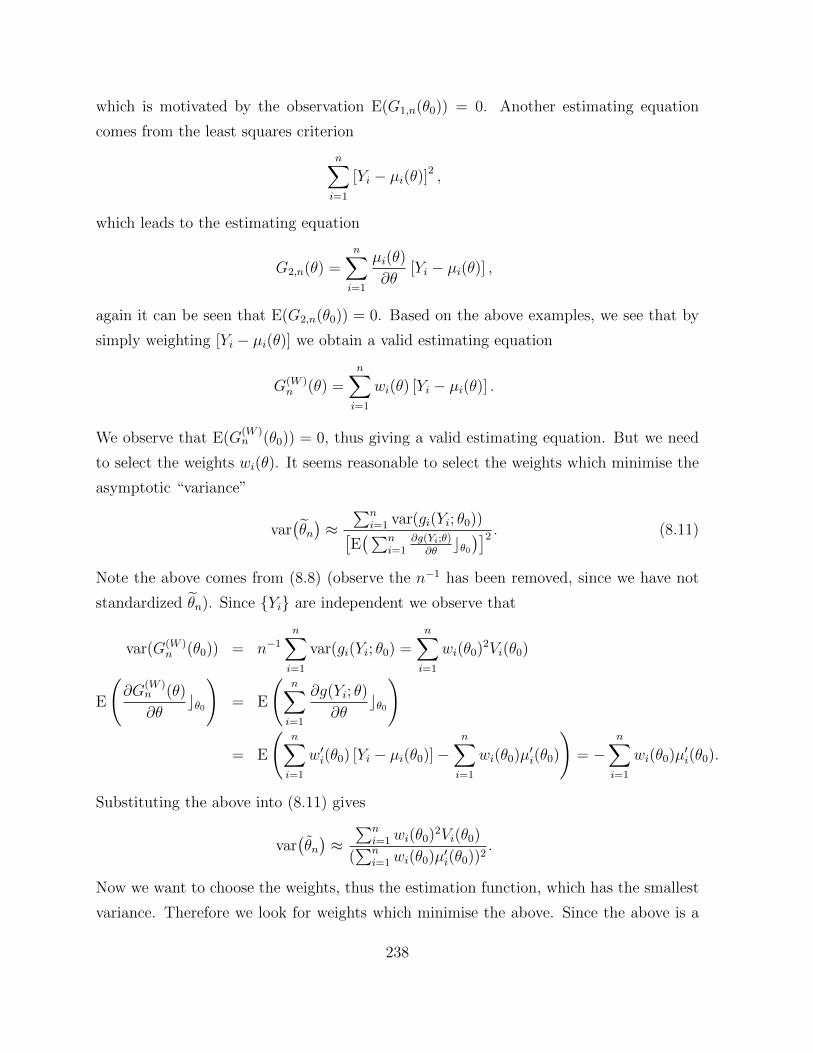
which is motivated by the observation E(G1,n(✓0)) = 0. Another estimating equation

comes from the least squares criterion

nX

i=1

[Yi � µi(✓)]2 ,

which leads to the estimating equation

G2,n(✓) =nX

i=1

µi(✓)

@✓[Yi � µi(✓)] ,

again it can be seen that E(G2,n(✓0)) = 0. Based on the above examples, we see that by

simply weighting [Yi � µi(✓)] we obtain a valid estimating equation

G(W )n (✓) =

nX

i=1

wi(✓) [Yi � µi(✓)] .

We observe that E(G(W )n (✓0)) = 0, thus giving a valid estimating equation. But we need

to select the weights wi(✓). It seems reasonable to select the weights which minimise the

asymptotic “variance”

var�

e✓n�

⇡Pn

i=1 var(gi(Yi; ✓0))⇥

E�

Pni=1

@g(Yi

;✓)@✓

c✓0�⇤2 . (8.11)

Note the above comes from (8.8) (observe the n�1 has been removed, since we have not

standardized e✓n). Since {Yi} are independent we observe that

var(G(W )n (✓0)) = n�1

nX

i=1

var(gi(Yi; ✓0) =nX

i=1

wi(✓0)2Vi(✓0)

E

@G(W )n (✓)

@✓c✓0

!

= E

nX

i=1

@g(Yi; ✓)

@✓c✓0

!

= E

nX

i=1

w0i(✓0) [Yi � µi(✓0)]�

nX

i=1

wi(✓0)µ0i(✓0)

!

= �nX

i=1

wi(✓0)µ0i(✓0).

Substituting the above into (8.11) gives

var�

✓n�

⇡Pn

i=1 wi(✓0)2Vi(✓0)

(Pn

i=1 wi(✓0)µ0i(✓0))

2.

Now we want to choose the weights, thus the estimation function, which has the smallest

variance. Therefore we look for weights which minimise the above. Since the above is a

238

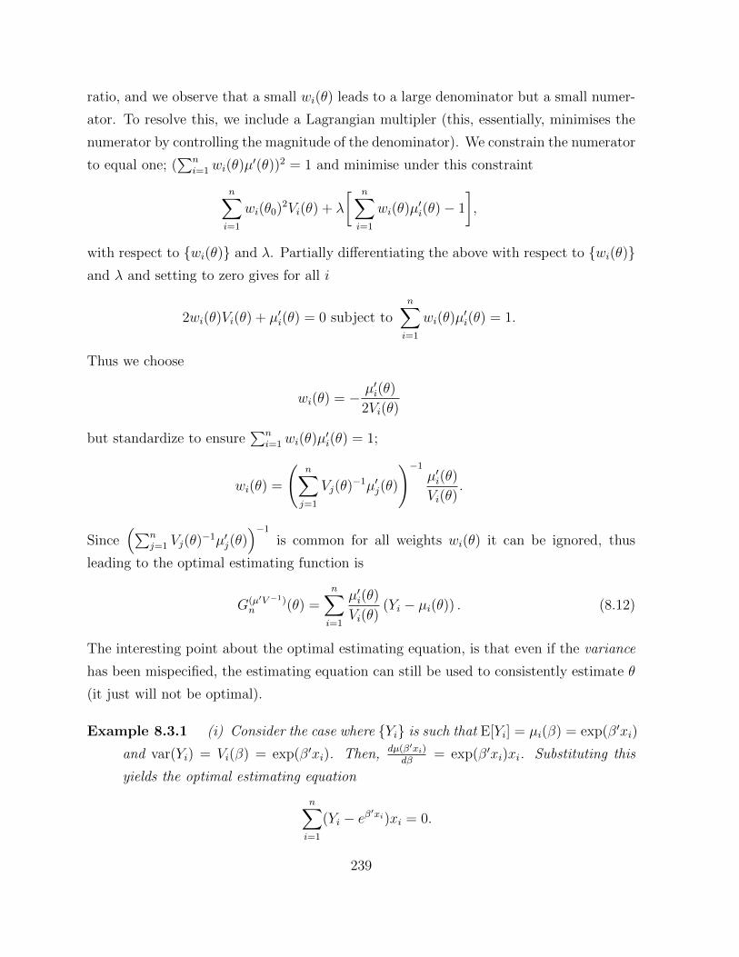
ratio, and we observe that a small wi(✓) leads to a large denominator but a small numer-

ator. To resolve this, we include a Lagrangian multipler (this, essentially, minimises the

numerator by controlling the magnitude of the denominator). We constrain the numerator

to equal one; (Pn

i=1 wi(✓)µ0(✓))2 = 1 and minimise under this constraint

nX

i=1

wi(✓0)2Vi(✓) + �

nX

i=1

wi(✓)µ0i(✓)� 1

�

,

with respect to {wi(✓)} and �. Partially di↵erentiating the above with respect to {wi(✓)}and � and setting to zero gives for all i

2wi(✓)Vi(✓) + µ0i(✓) = 0 subject to

nX

i=1

wi(✓)µ0i(✓) = 1.

Thus we choose

wi(✓) = � µ0i(✓)

2Vi(✓)

but standardize to ensurePn

i=1 wi(✓)µ0i(✓) = 1;

wi(✓) =

nX

j=1

Vj(✓)�1µ0

j(✓)

!�1µ0i(✓)

Vi(✓).

Since⇣

Pnj=1 Vj(✓)�1µ0

j(✓)⌘�1

is common for all weights wi(✓) it can be ignored, thus

leading to the optimal estimating function is

G(µ0V �1)n (✓) =

nX

i=1

µ0i(✓)

Vi(✓)(Yi � µi(✓)) . (8.12)

The interesting point about the optimal estimating equation, is that even if the variance

has been mispecified, the estimating equation can still be used to consistently estimate ✓

(it just will not be optimal).

Example 8.3.1 (i) Consider the case where {Yi} is such that E[Yi] = µi(�) = exp(�0xi)

and var(Yi) = Vi(�) = exp(�0xi). Then, dµ(�0xi

)d�

= exp(�0xi)xi. Substituting this

yields the optimal estimating equation

nX

i=1

(Yi � e�0x

i)xi = 0.

239

In general if E[Yi] = var[Yi] = µ(�0xi), the optimal estimating equation is

nX

i=1

[Yi � µ(�0xi)]

µ(�0xi)µ0(�0xi)xi = 0,

where we use the notation µ0(✓) = dµ(✓)d✓

. But it is interesting to note that when Yi

comes from a Poisson distribution (where the main feature is that the mean and

variance are equal), the above estimating equation corresponds to the score of the

likelihood.

(ii) Suppose {Yi} are independent random variables where E[Yi] = µi(�) and var[Yi] =

µi(�)(1 � µi(�)) (thus 0 < µi(�) < 1). Then the optimal estimating equation

corresponds to

nX

i=1

[Yi � µ(�0xi)]

µ(�0xi)[1� µ(�0xi)]µ0(�0xi)xi = 0,

where we use the notation µ0(✓) = dµ(✓)d✓

. This corresponds to the score function of

binary random variables. More of this in the next chapter!

Example 8.3.2 Suppose that Yi = �iZi where �i and Zi are positive, {Zi} are iid random

variables and the regressors xi influence �i through the relation �i = exp(�0 + �01xi). To

estimate �0 and �1 we can simply take logarithms of Yi

log Yi = �0 + �01xi + logZi.

Least squares can be used to estimate �0 and �1. However, care needs to be taken since in

general E[logZi] 6= 0, this will mean the least squares estimator of the intercept �0 will be

biased, as it estimates �0 + E[logZi].

Examples where the above model can arise is Yi = �iZi where {Zi} are iid with ex-

ponential density f(z) = exp(�z). Observe this means that Yi is also exponential with

density ��1i exp(�y/�i).

Remark 8.3.1 (Weighted least squares) Suppose that E[Yi] = µi(✓) and var[Yi] =

Vi(✓), motivated by the normal distribution, we can construct the weighted least squared

criterion

Ln(✓) =nX

i=1

1

Vi(✓)(Yi � µi(✓))

2 + log Vi(✓)

�

.

240

Taking derivatives, we see that this corresponds to the estimating equation

Gn(✓) =nX

i=1

� 2

Vi(✓){Yi � µi(✓)}

dµi(✓)

d✓� 1

Vi(✓)2{Yi � µi(✓)}2

dVi(✓)

d✓+

1

Vi(✓)

dVi(✓)

d✓

�

= G1,n(✓) +G2,n(✓)

where

G1,n(✓) = �2nX

i=1

1

Vi(✓){Yi � µi(✓)}

dµi(✓)

d✓

G2,n(✓) = �nX

i=1

1

Vi(✓)2{Yi � µi(✓)}2

dVi(✓)

d✓� 1

Vi(✓)

dVi(✓)

d✓

�

.

Observe that E[G1,n(✓0)] = 0 and E[G2,n(✓0)] = 0, which implies that E[Gn(✓0)] = 0. This

proves that the true parameter ✓0 corresponds to either a local minimum or saddle point

of the weighted least squares criterion Ln(✓). To show that it is the global minimum one

must use an argument similar to that given in Section 8.2.3.

Remark 8.3.2 We conclude this section by mentioning that one generalisation of esti-

mating equations is the generalised method of moments. We observe the random vectors

{Yi} and it is known that there exist a function g(·; ✓) such that E(g(Yi; ✓0)) = 0. To

estimate ✓0, rather than find the solution of 1n

Pni=1 g(Yi; ✓), a matrix Mn is defined and

the parameter which mimimises

1

n

nX

i=1

g(Yi; ✓)

!0

Mn

1

n

nX

i=1

g(Yi; ✓)

!

is used as an estimator of ✓.

241

242