lecture 5. rate variation, protein models, likelihood and...
TRANSCRIPT

Lecture 5. Rate variation, protein models, likelihood andBayesian methods. HMMs.
Joe Felsenstein
Department of Genome Sciences and Department of Biology
Lecture 5. Rate variation, protein models, likelihood and Bayesian methods. HMMs. – p.1/34

Rate variation among sites
In reality, rates of evolution are not constant among sites.
Lecture 5. Rate variation, protein models, likelihood and Bayesian methods. HMMs. – p.2/34

Rate variation among sites
In reality, rates of evolution are not constant among sites.
Fortunately, in the transition probability formulas, rates come in assimple multiples of times
Prob (i | j, u, t) = Prob (i | j, 1, ut)
Thus if we know the rates at two sites, we can compute theprobabilities of change by simply, for each site, multiplying all branchlengths by the appropriate rate
Lecture 5. Rate variation, protein models, likelihood and Bayesian methods. HMMs. – p.2/34

(continued ...)
If we don’t know the rates, we can imagine averaging them over adistribution f(u) of rates. Usually the Gamma distribution is used
Prob (i | j, t) =
∫∞
0
f(u) Prob (i | j, u, t) du
Lecture 5. Rate variation, protein models, likelihood and Bayesian methods. HMMs. – p.3/34

(continued ...)
If we don’t know the rates, we can imagine averaging them over adistribution f(u) of rates. Usually the Gamma distribution is used
Prob (i | j, t) =
∫∞
0
f(u) Prob (i | j, u, t) du
In practice a discrete histogram of rates approximates theintegration
Lecture 5. Rate variation, protein models, likelihood and Bayesian methods. HMMs. – p.3/34

(continued ...)
If we don’t know the rates, we can imagine averaging them over adistribution f(u) of rates. Usually the Gamma distribution is used
Prob (i | j, t) =
∫∞
0
f(u) Prob (i | j, u, t) du
In practice a discrete histogram of rates approximates the integration
(For the Gamma it seems best to use Generalized LaguerreQuadrature to pick the rates and frequencies in the histogram).
Also, there are actually autocorrelations with neighboring siteshaving similar rates of change.
This can be handled by Hidden Markov Models, which we coverlater.
Lecture 5. Rate variation, protein models, likelihood and Bayesian methods. HMMs. – p.3/34

A pioneer of protein evolution
Margaret Dayhoff, about 1966
Lecture 5. Rate variation, protein models, likelihood and Bayesian methods. HMMs. – p.4/34

Models of amino acid change in proteins
There are a variety of models put forward since the mid-1960’s:
1. Amino acid transition matricesDayhoff (1968) model. Tabulation of empirical changes inclosely related pairs of proteins, normalized. The PAM100matrix, for example, is the expected transition matrix given 1substitution per position.Jones, Taylor and Thornton (1992) recalculated PAM matrices(the JTT matrix) from a much larger set of data.Jones, Taylor, and Thornton (1994a, 1994b) have tabulated aseparate mutation data matrix for transmembrane proteins.Koshi and Goldstein (1995) have described the tabulation offurther context-dependent mutation data matrices.Henikoff and Henikoff (1992) have tabulated the BLOSUMmatrix for conserved motifs in gene families.
2. Goldman and Yang (1994) pioneered codon-based models (seenext screen).
Lecture 5. Rate variation, protein models, likelihood and Bayesian methods. HMMs. – p.5/34

Approaches to protein sequence models
Use a good model of DNA evolution.
Lecture 5. Rate variation, protein models, likelihood and Bayesian methods. HMMs. – p.6/34

Approaches to protein sequence models
Use a good model of DNA evolution.
Use the appropriate genetic code.
Lecture 5. Rate variation, protein models, likelihood and Bayesian methods. HMMs. – p.6/34

Approaches to protein sequence models
Use a good model of DNA evolution.
Use the appropriate genetic code.
When an amino acid changes, accept that change with a probabilitythat is smaller, the more different the two amino acids are in theirchemical properties (size, hydrophobicity etc.)
Fit this to empirical information on protein evolution.
Take into account variation of rates among sites, by allowingvariation in rates of acceptance of changes.
Take into account correlation of rates of change in neighboring sitesby having the acceptance rate change by an HMM.
How about protein structure? (as secondary structure? as 3Dstructure?)
Lecture 5. Rate variation, protein models, likelihood and Bayesian methods. HMMs. – p.6/34
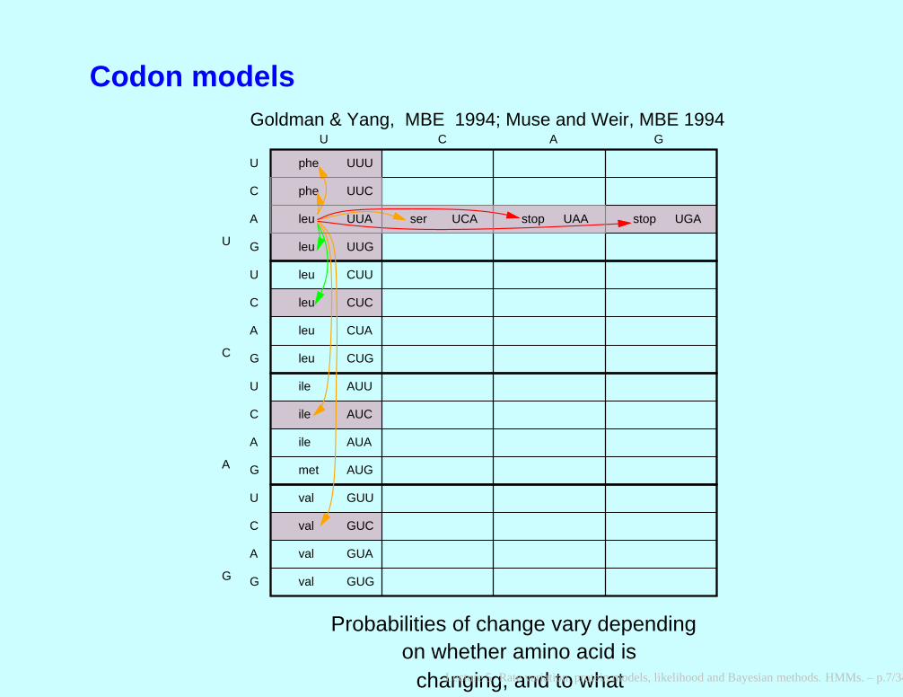
Codon models
U C A G
U
C
A
G
phe
phe
leu
leu
leu
leu
leu
leu
ile
ile
ile
met
val
val
val
val
ser stop stop
U
C
C
U
U
C
A
G
A
G
A
G
U
C
A
G
UUU
UUC
UUA
UUG
CUU
CUC
CUA
CUG
AUU
AUC
AUA
AUG
GUU
GUC
GUA
GUG
UCA UAA UGA
changing, and to what
Probabilities of change vary dependingon whether amino acid is
Goldman & Yang, MBE 1994; Muse and Weir, MBE 1994
Lecture 5. Rate variation, protein models, likelihood and Bayesian methods. HMMs. – p.7/34

Covarion models?
A G T A A G G T T T A A G T C A
A G A A G G T T T A A G T C A
A G A A G T T T A A G T C A
A G A A G G T T T A A G T C A
A G A A G T T T A A G T C A
A G A A G G T T A A G T C A
(Fitch and Markowitz, 1970)
C
AC
A
A
T
T
T
Which sites are available
for substitutions changes
as one moves along the tree
Lecture 5. Rate variation, protein models, likelihood and Bayesian methods. HMMs. – p.8/34

Likelihoods and odds ratios
Bayes’ Theorem relates prior and posterior probabilities of an hypothesisH:
Prob (H|D) = Prob (H and D)/ Prob (D)= Prob (D|H) Prob (H)/ Prob (D)
The ratios of posterior probabilities of two hypotheses, H1 and H2, put thisinto its “odds ratio” form ( Prob (D) cancels):
Prob (H1|D)
Prob (H2|D)=
Prob (D|H1)
Prob (D|H2)
Prob (H1)
Prob (H2)
Note that this says that the posterior odds in favor of H1 over H2 are theproduct of the prior odds and a likelihood ratio. The likelihood of thehypothesis H is the probability of the observed data given it,( Prob (D | H) ). This is not the same as the probability of the hypothesisgiven the data. That is the posterior probability of H and requires that wealso have a believable prior probability ( Prob (H) )
Lecture 5. Rate variation, protein models, likelihood and Bayesian methods. HMMs. – p.9/34

Rationale of likelihood inference
If the data consists of n items that are conditionally independent given thehypothesis i,
Prob (D|Hi)
= Prob (D(1)|Hi) Prob (D(2)|Hi) . . . Prob (D(n)|Hi).
and we can then write the likelihood ratio as a product of ratios:
Prob (D|H1)
Prob (D|H2)=
n∏
j=1
Prob (D(j)|H1)
Prob (D(j)|H2)
If the amount of data is large the likelihood ratio terms will dominate andpush the result towards the correct hypothesis. This can console ussomewhat for the lack of a believable prior.
Lecture 5. Rate variation, protein models, likelihood and Bayesian methods. HMMs. – p.10/34

Properties of likelihood inference
Likeihood inference has (usually) properties of
Consistency. As the number of data items n gets large, we convergeto the correct hypothesis with probability 1.
Efficiency. Asymptotically, the likelihood estimate has the smallestpossible variance (it need not be best for any finite number n of datapoints).
Lecture 5. Rate variation, protein models, likelihood and Bayesian methods. HMMs. – p.11/34

A simple example – coin tossing
If we toss a coin which has heads probability p and get HHTTHTHHTTT thelikelihood is
L = Prob (D|p)
= pp(1 − p)(1 − p)p(1 − p)pp(1 − p)(1 − p)(1 − p)
= p5(1 − p)6
so that trying to maximize it we get
dL
dp= 5p4(1 − p)6 − 6p5(1 − p)5
Lecture 5. Rate variation, protein models, likelihood and Bayesian methods. HMMs. – p.12/34

finding the ML estimate
and searching for a value of p for which the slope is zero:
dL
dp= p4(1 − p)5 (5(1 − p) − 6p) = 0
which has roots at 0, 1, and 5/11
Lecture 5. Rate variation, protein models, likelihood and Bayesian methods. HMMs. – p.13/34
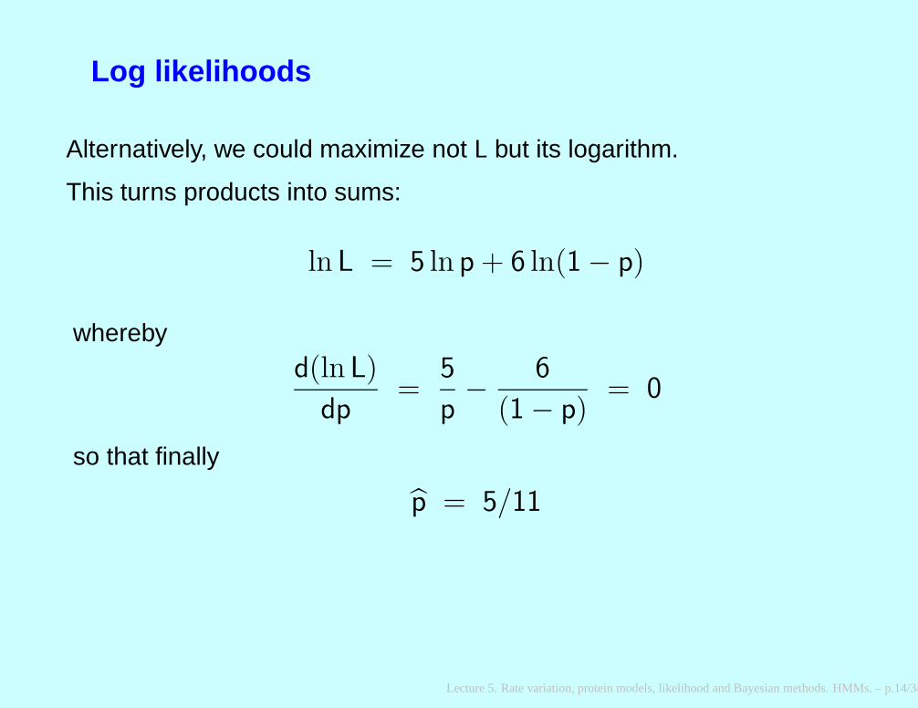
Log likelihoods
Alternatively, we could maximize not L but its logarithm.
This turns products into sums:
ln L = 5 ln p + 6 ln(1 − p)
wherebyd(ln L)
dp=
5
p−
6
(1 − p)= 0
so that finally
p̂ = 5/11
Lecture 5. Rate variation, protein models, likelihood and Bayesian methods. HMMs. – p.14/34
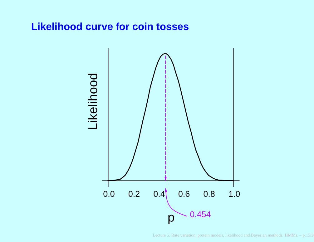
Likelihood curve for coin tosses
0.0 0.2 0.4 0.6 0.8 1.0
Like
lihoo
d
p 0.454
Lecture 5. Rate variation, protein models, likelihood and Bayesian methods. HMMs. – p.15/34

Likelihood on trees
AC
C
C G
x
z
w
t 1 t 2
t 3
t 4 t 5
t 6t 7
t 8
y
A tree, with branch lengths, and the data at a single site Thisexample is used to describe calculation of the likelihood
Since the sites evolve independently on the same tree,
L = Prob (D|T) =
m∏
i=1
Prob(D(i)|T
)
Lecture 5. Rate variation, protein models, likelihood and Bayesian methods. HMMs. – p.16/34

Likelihood at one site on a tree
We can compute this by summing over all assignments of statesx, y, z and w to the interior nodes
Prob(D(i)|T
)=
∑x
∑y
∑z
∑w
Prob (A,C,C,C,G, x, y, z,w|T)
Lecture 5. Rate variation, protein models, likelihood and Bayesian methods. HMMs. – p.17/34

Computing the terms
For each combination of states, the Markov process allows us to expressit as a product of probabilities of a series of changes, with the probabilitythat we start in state x:
Prob (A, C, C, C, G, x, y, z, w|T) =
Prob (x) Prob (y|x, t6) Prob (A|y, t1) Prob (C|y, t2)
Prob (z|x, t8) Prob (C|z, t3)
Prob (w|z, t7) Prob (C|w, t4) Prob (G|w, t5)
Lecture 5. Rate variation, protein models, likelihood and Bayesian methods. HMMs. – p.18/34

Computing the terms
Summing this up, there are 256 terms in this case:
∑x
∑y
∑z
∑w
Prob (x) Prob (y|x, t6) Prob (A|y, t1) Prob (C|y, t2)
Prob (z|x, t8) Prob (C|z, t3)
Prob (w|z, t7) Prob (C|w, t4) Prob (G|w, t5)
Lecture 5. Rate variation, protein models, likelihood and Bayesian methods. HMMs. – p.19/34
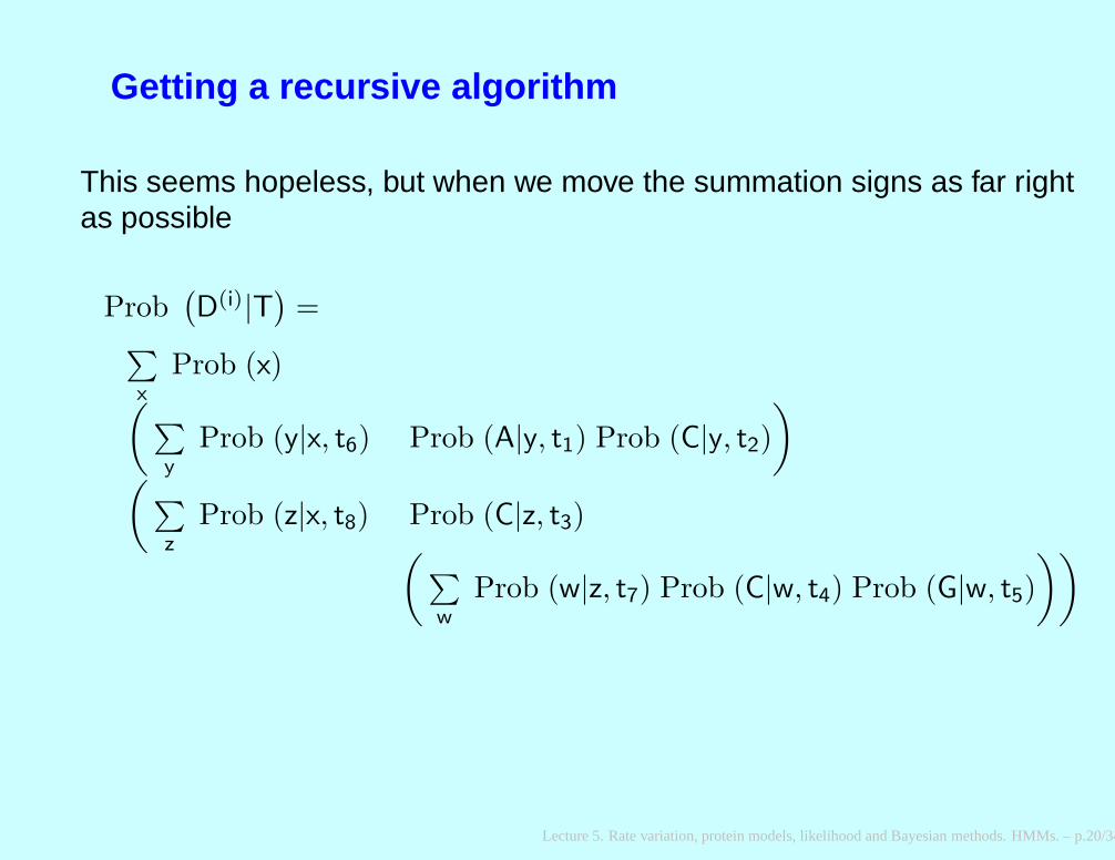
Getting a recursive algorithm
This seems hopeless, but when we move the summation signs as far rightas possible
Prob(D(i)|T
)=
∑x
Prob (x)(∑
y
Prob (y|x, t6) Prob (A|y, t1) Prob (C|y, t2)
)
(∑z
Prob (z|x, t8) Prob (C|z, t3)(∑
w
Prob (w|z, t7) Prob (C|w, t4) Prob (G|w, t5)
))
Lecture 5. Rate variation, protein models, likelihood and Bayesian methods. HMMs. – p.20/34

The pruning algorithm
Note that the pattern of parentheses in the previous expression is the
(A, C) (C, (C, G))
If L(i)k (s) is the probability of everything that is observed from node k on
the tree on up, at site i , conditional on node k having state s , we canexpress
(∑
w
Prob (w|z, t7) Prob (C|w, t4) Prob (G|w, t5)
)
as: ∑w
Prob (w|z, t7) L7(w)
Lecture 5. Rate variation, protein models, likelihood and Bayesian methods. HMMs. – p.21/34

and the algorithm is:
Continuing with this we find that the following algorithm computes the k ’sfrom the ℓ and m above them,
L(i)k (s) =
(∑x
Prob (x|s, tℓ) L(i)ℓ
(x)
)
×
(∑y
Prob (y|s, tm) L(i)m (y)
)
Lecture 5. Rate variation, protein models, likelihood and Bayesian methods. HMMs. – p.22/34

Starting and finishing the recursion
At the top of the tree the definition of the L’s specifies that they look like
this(L(i)(A), L(i)(C), L(i)(G), L(i)(T)
)= (1, 0, 0, 0)
and at the bottom the likelihood for the whole site can be computed
simply by weighting by the equilibrium state probabilities
L(i) =∑
x
πxL(i)0 (x)
Lecture 5. Rate variation, protein models, likelihood and Bayesian methods. HMMs. – p.23/34
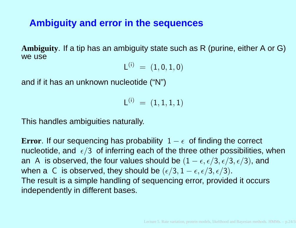
Ambiguity and error in the sequences
Ambiguity. If a tip has an ambiguity state such as R (purine, either A or G)we use
L(i) = (1, 0, 1, 0)
and if it has an unknown nucleotide (“N”)
L(i) = (1, 1, 1, 1)
This handles ambiguities naturally.
Error. If our sequencing has probability 1 − ǫ of finding the correctnucleotide, and ǫ/3 of inferring each of the three other possibilities, whenan A is observed, the four values should be (1 − ǫ, ǫ/3, ǫ/3, ǫ/3), andwhen a C is observed, they should be (ǫ/3, 1 − ǫ, ǫ/3, ǫ/3).The result is a simple handling of sequencing error, provided it occursindependently in different bases.
Lecture 5. Rate variation, protein models, likelihood and Bayesian methods. HMMs. – p.24/34

The tree is effectively unrooted
t6
before after
t6
6
80
86
The region around nodes 6 and 8 in the tree, when a new root(node 0) is placed in that branch
The subtrees are shown as shaded triangles
For the tree on the left of the figure above,
L(i) =∑
y
∑
z
∑
x
Prob (x) Prob (y|x, t6) Prob (z|x, t8).
Lecture 5. Rate variation, protein models, likelihood and Bayesian methods. HMMs. – p.25/34

using reversibility ...
Reversibility of the substitution process guarantees us that
Prob (x) Prob (y|x, t6) = Prob (y) Prob (x|y, t6).
Substituting, we get
L(i) =∑
y
∑
z
∑
x
Prob (y) Prob (x|y, t6) Prob (z|x, t8)
Finally we see that this is the same as the likelihood for a tree rooted atnode 8:
L(i)0 (z) = L
(i)8 (z) Prob (z) Prob (w|z, t6)L
(i)6 (w)
Lecture 5. Rate variation, protein models, likelihood and Bayesian methods. HMMs. – p.26/34

Finding the ML tree
So far I have just talked about the computation of the likelihood for onetree with branch lengths known.
As with the distance matrix methods, we must search the space of treetopologies, and for each one examined, we need to optimize the branchlengths to maximize the likelihood.
Lecture 5. Rate variation, protein models, likelihood and Bayesian methods. HMMs. – p.27/34

A numerical example
Squir MonkTarsier
Bovine
Lemur
HumanChimp
GorillaOrang
Gibbon
BarbMacaqCrab−E.Mac
Rhesus MacJpn Macaq
Mouse
A 232-nucleotide mitochondrial noncoding region data setover 14 species gives this ML tree with ln L = −2616.86
with a transition/transversion ratio of 30Lecture 5. Rate variation, protein models, likelihood and Bayesian methods. HMMs. – p.28/34
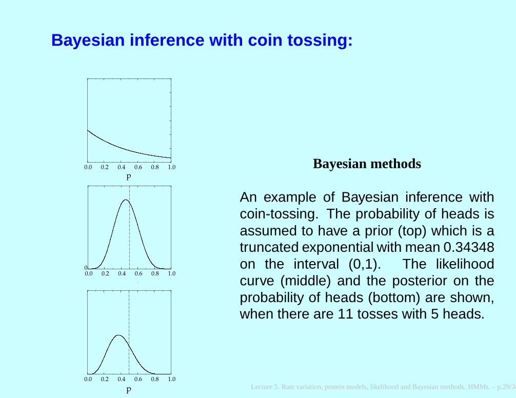
Bayesian inference with coin tossing:
0.0 0.2 0.4 0.6 0.8 1.0
p
0.0 0.2 0.4 0.6 0.8 1.00
0.0 0.2 0.4 0.6 0.8 1.0
p
Bayesian methods
An example of Bayesian inference withcoin-tossing. The probability of heads isassumed to have a prior (top) which is atruncated exponential with mean 0.34348on the interval (0,1). The likelihoodcurve (middle) and the posterior on theprobability of heads (bottom) are shown,when there are 11 tosses with 5 heads.
Lecture 5. Rate variation, protein models, likelihood and Bayesian methods. HMMs. – p.29/34

Bayesian phylogeny methods
Bayesian inference has been applied to inferring phylogenies (Rannalaand Yang, 1996; Mau and Larget, 1997; Li, Pearl and Doss, 2000).
All use a prior distribution on trees. The prior has enough influenceon the result that its reasonableness should be a major concern. Inparticular, the depth of the tree may be seriously affected by thedistribution of depths in the prior.
All use Markov Chain Monte Carlo (MCMC) methods (we willintroduce these in our discussion of coalescents) They sample fromthe posterior distribution.
When these methods make sense they not only get you a pointestimate of the phylogeny, they get you a posterior distribution ofpossible phylogenies.
Lecture 5. Rate variation, protein models, likelihood and Bayesian methods. HMMs. – p.30/34

References, page 1
Dayhoff, M. O. and R. V. Eck. 1968. Atlas of Protein Sequence and Structure1967-1968.National Biomedical Research Foundation, Silver Spring,Maryland. [Dayhoff’s PAM modelfor proteins]
Jones, D. T., W. R. Taylor, and J. M. Thornton. 1992. The rapid generation ofmutation data matrices from protein sequences. Computer Applcations inthe Biosciences (CABIOS)8: 275-282. [JTT model for proteins]
Jones, D. T., W. R. Taylor, and J. M. Thornton. 1994a. A model recognitionapproach to the prediction of all-helical membrane protein structure andtopology. Biochemistry33: 3038-3049. [JTT membrane protein model]
Jones, D. T., W. R. Taylor, and J. M. Thornton. 1994b. A mutation data matrixfor transmembrane proteins. FEBS Letters339: 269-275 . [JTT membraneprotein model]
Henikoff, S. and J. G. Henikoff. 1992. Amino acid substitution matrices fromprotein blocks. Proceedings of the National Academy of Sciences, USA89:10915-10919. [BLOSUM protein model]
Lecture 5. Rate variation, protein models, likelihood and Bayesian methods. HMMs. – p.31/34

References, page 2
Koshi, J. M. and R. A. Goldstein. 1995. Context-dependent optimalsubstitution matrices. Protein Engineering8: 641-645. [Generating otherkinds of protein model matrices]
Fitch, W. M. and E. Markowitz. 1970. An improved method for determi ningcodon variability in a gene and its application to the rate of fixation ofmutations in evolution. Biochemical Genetics4: 579-593. [The firstsuggestion of a covarion model]
Muse, S. V. and B S. Gaut. 1994. A likelihood method for comparingsynonymous and nonsynonymous nucleotide substitution rates, withapplication to the chloroplast genome. Molecular Biology and Evolution11:715-724. [One of the two introductions of the codon model]
Goldman, N. and Z. Yang. 1994. A codon-based model of nucleotidesubstitution for protein-coding DNA sequences. Molecular Biology andEvolution11: 725-736 [One of the two introductions of the codon model]
Fisher, R. A. 1912. On an absolute criterion for fitting frequency curves.Messenger of Mathematics41: 155-160. [First modern paper introducinglikelihood]
Lecture 5. Rate variation, protein models, likelihood and Bayesian methods. HMMs. – p.32/34

References, page 3
Fisher, R. A. 1922. On the mathematical foundations of theoretical statistics.Philosophical Transactions of the Royal Society of London,A 222: 309-368.[Likelihood in generality]
Neyman, J. 1971. Molecular studies of evolution: a source of novel statisticalproblems. pp. 1-27 in Statistical Decision Theory and Related Topics,ed. S.S. Gupta and J. Yackel. Academic Press, New York. [First application oflikelihood to molecular sequences]
Kashyap, R. L., and S. Subas. 1974. Statistical estimation of parameters in aphylogenetic tree using a dynamic model of the substitutional process.Journal of Theoretical Biology47: 75-101. [Second paper applyinglikelihood to molecular sequences]
Edwards, A. W. F., and L. L. Cavalli-Sforza. 1964. Reconstruction ofevolutionary trees. pp. 67-76 in Phenetic and Phylogenetic Classification,ed.V. H. Heywood and J. McNeill. Systematics Association Publ. No. 6,London. [First paper on likelihood for phylogenies]
Felsenstein, J. 1973. Maximum likelihood and minimum-steps methods forestimating evolutionary trees from data on discrete characters. SystematicZoology22: 240-249. [The “pruning” algorithm]
Lecture 5. Rate variation, protein models, likelihood and Bayesian methods. HMMs. – p.33/34
References, page 4
Felsenstein, J. 1981. Evolutionary trees from DNA sequences: a maximumlikelihood approach. Journal of Molecular Evolution17: 368-376. [Madelikelihood practical for n species]
Li, S., D. Pearl, and H. Doss. 2000. Phylogenetic tree construction usingMarkov chain Monte Carlo. Journal of the American Statistical Association95:493-508. [Bayesian inference of phylogenies by MCMC]
Mau, B., M. A. Newton, and B. Larget. 1997. Bayesian phylogenetic inferencevia Markov chain Monte Carlo methods. Molecular Biology and Evolution14: 717-724. [Bayesian inference of phylogenies by MCMC]
Rannala, B. and Z. Yang. 1996. Probability distribution of molecularevolutionary trees: a new method of phylogenetic inference. J. MolecularEvolution43: 304-311. [Bayesian inference of phylogenies by MCMC]
Felsenstein, J. 2004. Inferring Phylogenies.Sinauer Associates, Sunderland,Massachusetts. [material is in chapters 13, 14, 16]
Yang, Z. 2006. Computational Molecular Evolution. Oxford University Press,Oxford. [material is in pages 89-93, and chapters 1, 2]
Semple, C. and M. Steel. 2003. Phylogenetics.Oxford University Press,Oxford. [Material is in pages 145-160 and chapter 8]
Lecture 5. Rate variation, protein models, likelihood and Bayesian methods. HMMs. – p.34/34