chapter 8 pure competition -...

1

8.0 Preliminaries

In this chapter we combine the concepts and tools we developed in previous chapters dealing with demand, production, costs and market structure in order to analyze the behavior patterns of the market configurations that make up a modern economy. We ask: what happens (i.e., what are the outcomes) in purely competitive, monopolistically competitive, oligopolistic and monopolistic industries? We start with pure competition, which lies at the most competitive end of our scale measuring degrees of competitiveness. Also, as in Chapters 5 and 6, we ask in each case: Is this a short-run or a long-run analysis? We usually start with the short run.

REM 8.1: A purely competitive industry is one with many firms which are price takers; no single firm is able to determine the market price, there are no entry barriers, the product is homogeneous and there is no nonprice competition. Because of these characteristics a firm in such an industry faces a perfectly elastic demand curve. We pointed out in Chapter 7 that there are few industries in the United States and in other developed economies that fit this description.

QUESTION 8.1: If few industries have the characteristics of pure competition, why do we devote time and energy to analyzing the behavior of this market type?

ANSWER 8.1: There are three main reasons:

(1) Pure competition is the simplest market structure to analyze; it therefore offers a convenient gateway for the introduction of a number of crucial economic concepts that apply not only to the purely competitive case but to the other market structures as well.

(2) Pure competition serves as a kind of “benchmark” in economic analysis. We show that in a certain (limited) sense pure competition is the most “efficient” market structure possible; therefore, when

Chapter 8

Pure Competition

2

we analyze other industry structures, e.g., monopoly, we compare them to pure competition and ask: in what way does this particular market type resemble or differ from the purely competitive case?.

(3) There are industries that do not meet the strict requirements of the definition of pure competition but they approximate those requirements more or less closely. Then the tools and concepts developed in this chapter can still be applied in a rough and ready way to the analysis of such industries.

COMMENT 8.1: To analyze any market structure we need, in addition to information about demand, production and costs, at least one more thing: we need to know what motivates the owners and/or managers of firms in these industries. We said in Chapter 7 that in real life such motivations may be highly complex, but the simplest and also the most realistic assumption is profit maximization: that is, we assume that the goal of owners and managers is to earn a profit which is as high as possible given all the circumstances which they face. We call this a behavioral assumption and we maintain this assumption throughout most of the rest of our discussion in this and subsequent chapters. (In the textbox below we use the capital Greek letter pi (Π) for profit.)

COMMENT 8.2: Economists view pure competitors as “hemmed in” from all sides: They can do nothing about the prices at which they sell their products (they are price takers); they can do nothing about the prices which they pay for inputs (they are usually “pure competitors” on the buyers’ side in input markets) and they are either too small to influence the technology of their industry or find no advantage in trying to do so. There is a single decision open to them: to choose their “profit-maximizing” output level. It is this choice that we study carefully in this chapter. It may seem like a relatively insignificant matter, but it turns out that many important issues emerge from an analysis of this apparently simple choice.

ASSUMPTION 8.1 Firms seek to maximize (economic) profit. In symbols:

max Π = TR − TC

3

8.1 The Profit-Maximizing Output Level in the Short Run: Total Revenue and Total Cost

We start with the simple accounting definition: Profit = TR − TC. To analyze the logic of profit maximization and the choice of the profit-maximizing output level we examine the relationship between total revenue (TR), total cost (TC) and the level of output (Q).

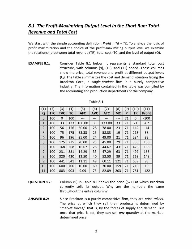
EXAMPLE 8.1: Consider Table 8.1 below. It represents a standard total cost structure, with columns (9), (10), and (11) added. These columns show the price, total revenue and profit at different output levels (Q). The table summarizes the cost and demand situation facing the Brockton Corp., a single-product firm in a purely competitive industry. The information contained in the table was compiled by the accounting and production departments of the company.

Table 8.1

(1) (2) (3) (4) (5) (6) (7) (8) (9) (10) (11)

Q TFC TVC TC AFC AVC ATC MC P TR Profit

0 100 0 100 --- --- --- --- 71 0 -100

1 100 33 133 100.00 33 133.00 33 71 71 -62

2 100 56 156 50.00 28 78.00 23 71 142 -14

3 100 75 175 33.33 25 58.33 19 71 213 38

4 100 96 196 25.00 24 49.00 21 71 284 88

5 100 125 225 20.00 25 45.00 29 71 355 130

6 100 168 268 16.67 28 44.67 43 71 426 158

7 100 231 331 14.29 33 47.29 63 71 497 166

8 100 320 420 12.50 40 52.50 89 71 568 148

9 100 441 541 11.11 49 60.11 121 71 639 98

10 100 600 700 10.00 60 70.00 159 71 710 10

11 100 803 903 9.09 73 82.09 203 71 781 -122

QUESTION 8.2: Column (9) in Table 8.1 shows the price ($71) at which Brockton currently sells its output. Why are the numbers the same throughout the entire column?

ANSWER 8.2: Since Brockton is a purely competitive firm, they are price takers. The price at which they sell their products is determined by “market forces,” that is, by the forces of supply and demand. But once that price is set, they can sell any quantity at the market-determined price.

4

PROBLEM 8.1: Jim Bitterman is in charge of production planning for Brockton. His job is to determine the company’s profit maximizing output level (Q*). How can he do this?

SOLUTION 8.1: Given the information in Table 8.1 this is easy: Inspect Column (11)

and find the output level at which maximum profit is achieved. This happens when 7 units are produced and we write: Q* = 7. So if a large amount of detailed information of the type contained in Table 8.1 is available (and we are dealing with a single-product firm!), the production decision is simple.

REM 8.2: When we say that Column (11) in Table 8.1 shows the level of “profit” we mean economic profit (or loss). The cost items shown in the table (and in FIG 8.1) include all the relevant opportunity costs including a normal profit. So profit means a surplus over and above those costs.

Now consider FIG 8.1below. It reproduces FIG 6.8 (and plots the data from Table 8.1) with the addition of a total revenue curve. This “curve” is a straight line with a positive slope starting at the origin since it plots the relationship TR = P x Q. When no production takes place TR = 0 and so the TR curve starts at the origin. Then, each time production (and sales) increase by one unit TR increases by the same amount (i.e., the price, $71). So it is clear that a pure competitor faces a linear total revenue curve.

FIG 8.1

TR

TC

TFC

TVC

5

QUESTION 8.3: How can you tell just by looking at Table 8.1 and FIG 8.1 that they involve short-run analysis?

ANSWER 8.3: Since both the table and the graph differentiate between fixed and variable costs, we know that they deal with short-run analysis.

PROBLEM 8.2: How can Jim Bitterman use FIG 8.1 to find the company’s profit-maximizing output level?

SOLUTION 8.2: Since profit = TR − TC he should search for the output level shown along the horizontal axis where the vertical distance between the total revenue curve and the total cost curve is at its maximum. This happens when Q = 7. (Note the arrow pointing to “7” on the horizontal axis.) So FIG 8.1 can be used to solve the company’s production problem graphically.

NOTE 8.1: Observe that there is a certain “family resemblance” between FIG 8.1 and a diagram which is widely used in break-even analysis. Jim Bitterman may need to know at what output level the Brockton Co. “breaks even,” i.e., total revenue is just high enough to cover total cost, where total cost includes all opportunity costs. This topic is discussed further below, but note that in FIG 8.1 there are two break-even points: TR = TC at output levels where the TC curve crosses the TR curve, and in FIG 8.1 this happens when Q ≈ 2.3 (see arrow) and when Q equals 10. Also note that if Q < 2.3 and Q > 10 Brockton suffers (economic) losses (TR < TC).

FIG 8.2

6

FIG 8.2, called the “Profit Curve,” plots the profit obtained by the Brockton Corp. at different output levels. The data come from Column (11) of Table 8.1 or from FIG 8.1. If Figure 8.1 is used, the graph plots the vertical distances between the TR and TC curves against the level of output. Logically then the two graphs contain the same information.

PROBLEM 8.3: How can Bitterman use FIG 8.2 to find Brockton’s profit-maximizing output level?

SOLUTION 8.3: Determining the profit-maximizing level of output from this graph is straightforward: Find the output at which the Profit Curve reaches its highest level. Clearly FIG 8.1 and FIG 8.2 give the same solution to Jim Bitterman’s problem, i.e., Q* ≈ 7.

Break-Even Analysis

Imagine that the Brockton Corp. has much less detailed information about its production process than is available in Table 8.1. This of course is often the case in real life. In fact, the accounting department is able to provide the production manager with only two numbers: Fixed costs are $100 and average variable cost is $25 when Q = 5. Given the known price (P = $71) and a bit of arithmetic, the graph shown in FIG 8.3, called a break-even diagram, can be plotted. It is based on the assumption that AVC is constant; hence the TVC curve is linear.

NOTE 8.2: Elementary geometry indicates that to draw a straight line you need two points. The TVC curve in FIG 8.3 is drawn through the origin (TVC = 0) and through the point (Q = 5, TVC = $125).

(The TC curve is obtained in the same way as in FIG 8.1, i.e., by adding the TVC and TFC curves.) Note again the family resemblance between FIG 8.1 and FIG 8.3.

QUESTION 8.4: What is the purpose of the break-even diagram (FIG 8.3)?

ANSWER 8.4: As the name implies, it enables firms to determine their “break-even” level of output, i.e., the output level at which they are just able to cover all their costs. At any higher output level they earn (economic) profits while at lower output levels they suffer (economic) losses. Note that this occurs at the intersection point between the TR curve and the TC curve, called the break-even point. It should be clear that we are discussing the economic break-even point: When we say the firm is “breaking even” we mean that they earn zero economic profit but they are earning a normal profit.

7

FIG 8.3

PROBLEM 8.4: The Brockton Corporation’s Jim Bitterman is engaged in production planning. He assumes that the market price will remain the same over the next production period but wants to make a “back-of-the-envelope” calculation to determine his minimum input requirements for that period. How can he do this?

SOLUTION 8.4: FIG 8.3 provides the answer. Unless Brockton obtains inputs that are at least sufficient to produce a bit over 2 units, the firm will not break even.

NOTE 8.3: We often assume that only “whole” units can be produced, e.g., 3 units but not 3.2 units. Then the answer to PROBLEM 8.4 would be somewhat different: Brockton must obtain inputs sufficient to produce at least 3 units.

NOTE 8.4: Observe that FIG 8.1 can also be thought of as a “break-even” diagram. But since the cost curves are nonlinear (REM: We derived them from a production function embodying the law of “eventually” diminishing returns) there are two break-even points! (Note the first arrow pointing to the interval between “2” and “3” and the third arrow pointing a bit to the right of “10.”) Positive profits are earned at output levels to the right of the first and to the

TC

TR

TVC

TFC

8

left of the second break-even point. Outside of that interval the firm incurs (economic) losses.

The Shut-Down Point: TR, TC and TVC

We have examined the problem of finding a firm’s (short-run) profit-maximizing output level. We now ask a related question: Should the firm produce anything at all, or would its owners be better off shutting down, i.e., cutting production to zero? We ask this question from both a short-run and a long-run perspective.

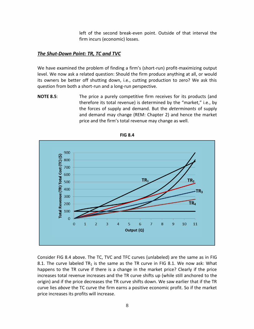
NOTE 8.5: The price a purely competitive firm receives for its products (and therefore its total revenue) is determined by the “market,” i.e., by the forces of supply and demand. But the determinants of supply and demand may change (REM: Chapter 2) and hence the market price and the firm’s total revenue may change as well.

FIG 8.4

Consider FIG 8.4 above. The TC, TVC and TFC curves (unlabeled) are the same as in FIG 8.1. The curve labeled TR1 is the same as the TR curve in FIG 8.1. We now ask: What happens to the TR curve if there is a change in the market price? Clearly if the price increases total revenue increases and the TR curve shifts up (while still anchored to the origin) and if the price decreases the TR curve shifts down. We saw earlier that if the TR curve lies above the TC curve the firm earns a positive economic profit. So if the market price increases its profits will increase.

TR1 TR2

TR3

TR4

9

REM 8.3: If a firm’s revenues exceed their economic costs they earn a surplus called economic or pure (or “above-normal”) profit. (Chapter 6.)

Interesting questions arise if the market price decreases. We show three possibilities in FIG 8.4:

(1) The market price decreases (to $44); the TR curve shifts down until it is just tangent to the TC curve, i.e., it just touches the TC curve at a single point. This is shown (in red) by TR2. There is one point where TR = TC, that is, there is one output level where revenues are just enough to cover total costs and the firm breaks even.

QUESTION 8.5: From either a short-run or a long-run perspective should the firm stay in business or should they shut down, i.e., cut production to zero?

ANSWER 8.5: Since the firm is breaking even in the economic sense they are earning a normal profit.

REM 8.4: Normal profit is defined as the minimum return required to keep the owners’ (or stockholders’) resources in their current activity. It is equivalent to the highest return those resources could earn in any alternative activity.

Since the firm is earning a normal profit they are earning as high a return in their present business as they could elsewhere. They therefore would/should stay in their present line of business both in the short run and the long run.

(2) The market price decreases (to $34); the TR curve shifts down until it lies everywhere below the TC curve but there is an interval in which it lies above the TVC curve (TVC < TR <TC). This is shown (in blue) by TR3. Revenues are enough to cover all variable costs and some part of fixed costs but not enough to cover all costs (including all relevant opportunity costs). In other words, the firm is suffering an economic loss.

QUESTION 8.6: What should they do in the short and long run?

ANSWER 8.6: In the short run they should produce despite an economic loss but in the long run they should cut production to zero (and “take their marbles and go elsewhere”).

10

Why should the firm produce in the short run despite an economic loss? The answer is that ASSUMPTION 8.1 is incomplete: firms seek maximum profits; but if they are unable to earn a profit they would/should at least try to minimize their losses!

In the short run fixed costs are unavoidable (the firm can do nothing about them), so logically they should be ignored in making short-run production decisions − only variable costs should be considered. If the firm were to shut down under these circumstances their loss would equal their total fixed cost. But if instead they keep on producing, revenues would be enough to cover total variable cost plus some portion of fixed cost so their losses would be smaller.

REM 8.5: The short-run is defined as a time period in which the level of use of at least one input cannot be changed; we call such an input a fixed input and the cost of such an input is a fixed cost. So in the short-run firms are “stuck” with these costs; hence we call them “unavoidable.” But variable costs are avoidable: If production ceases variable cost no longer need to be incurred.

We have reached an important conclusion which we will state as a decision rule.

NOTE 8.6: There is an obvious corollary to DECISION RULE 8.1: only variable costs, i.e., those under the control of the firm’s management should be considered in making short run economic decisions.

What about the long run? From a long-run perspective all costs are variable – there is enough time to change the level of use of all the inputs employed by the firm; they are not “stuck” with fixed costs. If revenues are not enough to cover all (opportunity) costs the owners of the firm can shift their resources elsewhere. So from a long-run perspective the best solution is to cut production to zero.

(3) The market price decreases (to $24); the TR curve shifts down until it is tangent to the TVC curve, i.e., it just touches the TVC curve at a single point (TR = TVC). This is shown (in brown) by TR4. Revenues are just enough to cover TVC.

DECISION RULE 8.1: When making (short-run) economic decisions fixed costs should be ignored.

11

QUESTION 8.7: What should they do in the short and long run?

ANSWER 8.7: If TR = TVC the firm is just able to cover its variable costs; so whether they keep on producing or shut down, their loss would equal their fixed costs. From a short-run perspective then they are just on the boundary between producing and not producing. They can decide which option to choose with a coin toss. From a long-run perspective the answer remains as before: Shut down if your revenues are not sufficient to cover all costs

(4) The market price decreases (to below $24); the TR curve shifts down until it lies everywhere below the TVC curve (not shown in FIG 8.4). Revenues are not enough to cover even variable costs.

QUESTION 8.8: What should they do in the short and long run? Explain.

ANSWER 8.8: The answer is left as an exercise for the reader.

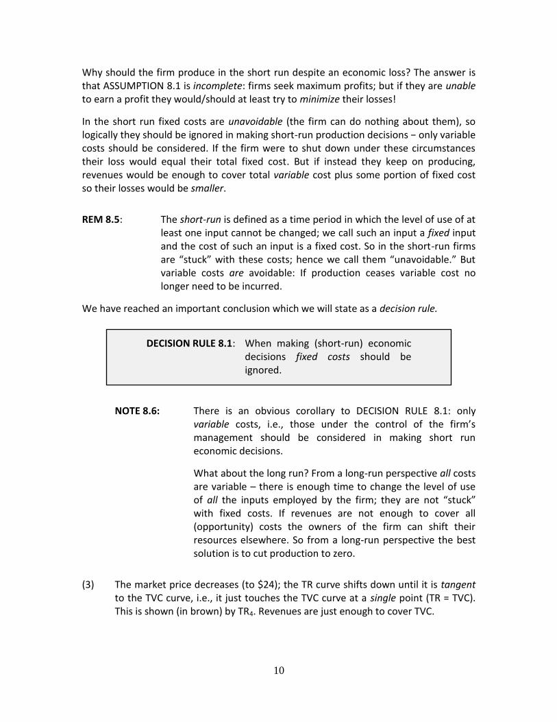
The conclusions of our discussions in this section are summarized in Table 8.2. The question mark means that management can decide whether to produce or not with a coin toss.

Table 8.2

If: In the Short-Run: In the Long Run

TR>TC produce produce

TR = TC produce produce

TVC<TR<TC produce don’t produce

TR = TVC produce (?) don’t produce

TR<TVC don’t produce don’t produce

Fixed Costs, Sunk Costs and Avoidable Costs in Decision-Making

The discussion in the previous section which led us to DECISION RULE 8.1 (“Ignore fixed costs in short-run decision making”) leads to a broader concept, that of sunk costs, which plays an important role in the economic analysis of decision-making.

DEF 8.1 Sunk Costs are costs which have been incurred in the past or for some other reason cannot be avoided.

12

EXAMPLE 8.2: The XLC Corp. is in the construction business in the Southwest and they are putting up an office complex “on speculation,” that is, they are building it not under contract as is usually the case in the construction business, but simply in the hope of selling it at a profit when it is completed. Due to the availability of modern accounting software they have “real time” information about their expenses. When the project is half-completed they find that up to that point their expenditures for labor, materials, leased equipment, fuel and some smaller items add up to $1.7 million. All of these expenses are sunk costs. Since they have already been incurred there is nothing XLC can do about them now.

EXAMPLE 8.3: The management of the King Kong Trading Co. expect to obtain a number of lucrative contracts from several domestic retailers and in preparation they sign leases for a large amount of warehouse space. Unfortunately negotiations for the largest of these contracts fall through and they end up needing much less warehouse space than they anticipated. The company’s lawyers tell them that the leases are tightly written and cannot be broken and that they do not permit subleasing (that is leasing the space to others). The lease payments (even though they have not yet occurred) are also sunk costs.

The contrasting concept is that of avoidable costs. (Some people call them incremental costs but we use that term somewhat differently later in this chapter.) Like variable costs, but unlike sunk costs avoidable costs are under the control of management (or other decision makers.) They can be avoided if a particular choice is not made.

EXAMPLE 8.4: The Kaycee Corp. is a diversified consumer products company. They are in the early planning stages of an advertising campaign with an estimated cost of $17 million. Before the decision is made to undertake such a campaign, the $17 million is an avoidable cost.

There is a great deal of overlap between the sunk costs and fixed costs concepts. Because fixed costs are independent of the firm’s output level and cannot be controlled by management in the short run they are similar to sunk costs. Sunk costs therefore play a role similar to fixed costs in economic (and noneconomic!) decision situations.

DEF 8.2: Avoidable costs are costs that can be avoided if a particular choice or decision is not made.

13

That is, we say that since sunk costs cannot be affected by a particular decision they should not affect that decision. The point can be summed up in a decision rule:

QUESTION 8.9: The XLC Corp. (see EXAMPLE 8.2) expected the total cost of the project to be $3.5 million and to be able to sell the complex for at least $5 million. Their costs are on track but in the meantime the market for office space in the region has collapsed and the best price they can expect to get once the project is completed is $3 million. The top managers of the company are discussing the question of what to do about it.

Phil Johnson (C.E.O.): “We cannot bail out in the middle of a project. We have already spent $1.7 million on it. “

Andy Forrester (C.F.O.): “If we continue the project we will end up with half a million in losses.”

Who is right, Johnson or Forrester?

ANSWER 8.9: Neither! The $1.7 million that has already been spent is irrelevant. It is a sunk cost and should be ignored. The only relevant numbers are the $1.8 million that still must be spent (an avoidable cost) and the $3 million for which the completed project can be sold.

8.2 The Profit-Maximizing Output Level in the Short Run: Marginal Revenue and Marginal Cost

There is an alternative approach to the question we asked in Section 8.1 about a firm’s profit-maximizing output level. It involves the use of marginal as opposed to total quantities. The two approaches are logically identical but the marginal approach helps us gain important insights into both business and nonbusiness decision making.

Consider FIG 8.5. It reproduces FIG 8.2 (and plots the data from Columns (6), (7) and (8) of Table 8.1) with the addition of the horizontal line labeled P, MR. This line is the “demand curve” facing the Brockton Corp. It is perfectly elastic and drawn at the level of the current market price (P = $71; note the arrow along the vertical axis.) So FIG 8.5

DECISION RULE 2: Sunk costs should be ignored in making economic (and many noneconomic) decisions.

14

depicts the demand and cost situation facing the Brockton Corp. expressed on a per unit basis.

FIG 8.5

QUESTION 8.10: Why is the demand curve facing Brockton perfectly elastic?

ANSWER 8.10: Since Brockton is a firm in a purely competitive industry they are price takers. At the market-determined price they can sell any amount they wish but if they attempt to charge a higher price their sales would drop to zero. They have no reason to charge a lower price but if they did their sales would grow to “infinity.” The result is the horizontal, perfectly elastic demand curve we see in FIG 8.5.

To use FIG 8.5 to determine Brockton’s profit-maximizing output level we need a new concept called marginal revenue (MR).

P, MR

ATC

AVC

MC

15

NOTE 8.7: The MR concept provides an answer to the following question: If we produce and sell a little bit more, say one more unit, how much extra revenue would we receive? It is therefore similar to the other “marginal” concepts we encountered in previous chapters.

NOTE 8.8: The MR concept is particularly simple for a purely competitive firm: If they produce and sell one additional unit, the extra revenue they receive is just the price. (This is not the case in other market structures!) For firms in purely competitive industries (but only for such firms!) we can therefore write:

It is for this reason that the demand curve in FIG 8.5 is labeled P, MR so we will sometimes call it the “marginal revenue (MR) curve” and sometimes the “price line” (and sometimes the “demand curve”).

We now have the tools to answer the question we stated at the beginning of this section: What is the Brockton Corp.’s profit-maximizing output level? The answer is given by the following decision rule:

In FIG 8.5 this output level occurs at the intersection between the MR curve and the MC curve and the answer is again Q* = 7; (note the arrow pointing to “7” on the horizontal axis). This should come as no surprise since, as we pointed out the two approaches are logically identical.

DEF 8.3: Marginal Revenue (MR) is defined as the change in total revenue that results from a small (usually a one-unit) change in production and sales. In symbols:

ΔQ

ΔTRMR

In pure competitors MR = P

DECISION RULE 8.3: Produce up to the point where MR = MC

16

QUESTION 8.11: Why is “MR = MC” the proper decision rule?

ANSWER 8.11: Imagine that Jim Bitterman, the production manager, tries to arrive at the answer by “trial-and-error.” He writes a small program on his laptop that tells him for each possible output level, produce “more,” produce “less” or “stop,” you have found the profit-maximizing output level. He starts with an output below 7, say Q = 5. The marginal revenue of course equals the price (P = $71) and the marginal cost equals $29. (The numbers come from Table 8.1) What will his little program tell him? Produce more, since by doing so you will add more to your revenues than to your costs, so profits will increase. In other words, as long as MR > MC (the MR line lies above the MC curve in Figure 8.5), increase production. He next experiments with an output higher than 7, say Q = 9. MR still equals $71 but now MC = $121. The program will say produce less, since by doing so you will lower your costs more than your revenues and again profits will increase. So when MR < MC (the MR line lies below the MC curve) reduce production. But when MR = MC there is no gain from either increasing or decreasing production. It is time to “stop,” since you have found the profit-maximizing output level. This analysis is summarized in Table 8.3

Table 8.3

Output Situation Action

5 MR>MC produce more!

7 MR = MC stop!

9 MR<MC produce less!

QUESTION 8.12: Can Jim Bitterman solve the problem of finding the profit-maximizing output level by using the per-unit data in Table 8.1?

ANSWER 8.12: Yes. He can inspect Columns (8) and (9) which show the marginal costs and price (marginal revenue) facing the company and find the output level where MR (=P) = MC. Unfortunately there is no place in the table where the price is exactly equal to marginal cost. So if we insist that only whole units (i.e., no fractional units) can be produced, the rule must be modified:

DECISION RULE 8.3’: Produce up to the point where MR ≥ MC; (but make sure that MR and MC are as close as possible!)

17

Applying this rule we again come up with Q* = 7.

QUESTION 8.13: To test your understanding of the MR = MC rule ask the following question: What if Bitterman decides to produce 6 units instead of 7? Why is this a mistake?

ANSWER 8.13: Because if the company increases its output from Q = 6 to Q = 7 the added revenue is $71 (i.e., the price or marginal revenue), the added cost is $63 (the marginal cost) so the added profit is $8 ($72 − $63). By producing only 6 units Brockton Corp. gives up $8 in potential profit. (The data again come from Table 8.1)

QUESTION 8.14: What if Bitterman decides to produce 8 units instead of 7? Why is this a mistake?

ANSWER 8.14: The answer to this question is left as an exercise for the reader.

QUESTION 8.15: Bitterman’s assistant, Fred Cook, claims that the profit-maximizing output level occurs in FIG 8.5 where the ATC curve reaches its lowest point because this is where the vertical distance between P and ATC is at its maximum. It is found at the output level where the MC curve cuts the ATC curve. (Note the arrow pointing to the interval between “5” and “6” in FIG 8.5.)

REM 8.5: The MC curve crosses the ATC curve at its minimum point. (Chapter 6).

So Cook’s “decision rule” looks like this:

Why is this incorrect?

ANSWER 8.15: Something in fact is maximized at this output level, namely profit per unit. But ASSUMPTION 8.1 states that firms seek to maximize total profit. The two are not necessarily the same, as illustrated in the table below.

max (P − ATC)

18

Table 8.4

Q P ATC Profit/Q Total Profit

$5 $71 $45.00 $26.00 $130

6 71 44.67 26.33 158

7 71 47.29 23.71 168

The data are extracted from Table 8.1 with the addition of a column showing profit per unit (P − ATC). It is clear from this table that if the company produces 5 or 6 units profit per unit is higher than at Q = 7 but total profit is lower.

The MR = MC rule is an example of the method called “marginal analysis” which we mentioned in earlier chapters. We pointed out that this approach is typically used in economics, especially in microeconomics. So while it is important to be familiar with and understand this rule, it is even more important to understand the logic behind it. So we approach the problem from a second, somewhat different perspective.

FIG 8.6

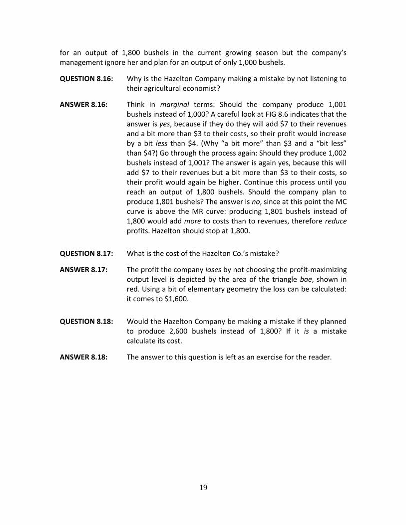
Consider FIG 8.6. It is a highly simplified version of FIG 8.5. The average cost curves are omitted and only the upsloping portion of the marginal cost curve is shown. (For simplicity we also assume that the marginal cost curve is linear.) It depicts the situation of the Hazelton Company, a large corporate farming operation in the Midwest. (It is large in absolute terms but small in relation to the markets it operates in.) The graph shows the wheat-growing part of Hazelton’s business. (The current price of wheat is $7 per bushel.) The company employs an agricultural economist who advises them to plan

Quantity 1,000 1,800 2,600 0

MR

MC

$/Q

7 a

b

11

3

c

d

e

19

for an output of 1,800 bushels in the current growing season but the company’s management ignore her and plan for an output of only 1,000 bushels.

QUESTION 8.16: Why is the Hazelton Company making a mistake by not listening to their agricultural economist?

ANSWER 8.16: Think in marginal terms: Should the company produce 1,001 bushels instead of 1,000? A careful look at FIG 8.6 indicates that the answer is yes, because if they do they will add $7 to their revenues and a bit more than $3 to their costs, so their profit would increase by a bit less than $4. (Why “a bit more” than $3 and a “bit less” than $4?) Go through the process again: Should they produce 1,002 bushels instead of 1,001? The answer is again yes, because this will add $7 to their revenues but a bit more than $3 to their costs, so their profit would again be higher. Continue this process until you reach an output of 1,800 bushels. Should the company plan to produce 1,801 bushels? The answer is no, since at this point the MC curve is above the MR curve: producing 1,801 bushels instead of 1,800 would add more to costs than to revenues, therefore reduce profits. Hazelton should stop at 1,800.

QUESTION 8.17: What is the cost of the Hazelton Co.’s mistake?

ANSWER 8.17: The profit the company loses by not choosing the profit-maximizing output level is depicted by the area of the triangle bae, shown in red. Using a bit of elementary geometry the loss can be calculated: it comes to $1,600.

QUESTION 8.18: Would the Hazelton Company be making a mistake if they planned to produce 2,600 bushels instead of 1,800? If it is a mistake calculate its cost.


20

QUESTION 8.19: Can we use FIG 8.5 (the unit-cost-price diagram) to determine total revenue, total cost and total profit if we know the current market price?

ANSWER 8.19: Yes. Consider FIG 8.7 below. It shows the Brockton Corp.’s unit costs and price (P = $71; note the “P” and the arrow along the vertical axis.) The price is also shown by the distance QR. As before, the profit-maximizing output is 7 units (note the “Q” and the arrow along the horizontal axis). Since TR = P x Q it is shown in the graph by the area of the rectangle OPRQ (TR = $71 x 7 = $497). Average total cost when 7 units are produced is shown by the vertical distance from the horizontal axis to the ATC curve, or the distance QT. When 7 units are produced ATC = $47.29 (See Table 24.1). Since TC = ATC x Q, the total cost at the firm’s profit-maximizing output level is shown by the area of the rectangle OSTQ. (TC = $47.29 x & = $331.03.) And since profit (Π) = TR − TC, the difference between these two rectangles shows the firms profit when the price is $71. (Π = $497 − $331.03 = $165.97.)

NOTE 8.9: We developed the MR = MC rule in the context of a firm in a purely competitive industry. But the rule is generally applicable: Whether the firm is a pure competitor, monopolistic competitor, oligopolist or pure monopolist, the profit-maximizing output level is found by using the same decision rule.

21

FIG 8.7

Incremental Analysis

The marginal approach which we have encountered in several places, but especially in this chapter with the development of the MR = MC rule, leads naturally to a broader type of analysis which is applicable to many different decision-making situations.

Imagine a decision-maker (an individual or a group) faced with a problem of choice: Should we undertake a particular project? Should we engage in a particular activity? Should we fix the roof on our headquarters building? Should we introduce a new product? Should the hospital acquire a new MRI machine? Should we raise our prices?

The information that the decision-maker should gather and the analytic tools that should be employed can get extremely expensive and complicated. But ultimately the process boils down to two questions: If we do this what will be the incremental revenue? What will be the incremental cost?

P R

S T

Q

ATC

AVC

MC

DEF 8.4: Incremental Revenue (IR) is defined as the change in revenue that results if a particular activity is undertaken.

22

EXAMPLE 8.5: The Baskerville Trucking Co. is considering a job to ship 120 tons of freight from Philadelphia to Jacksonville, FL at a rate of $140 per ton. If they accept the job the incremental revenue (IR) would be:

IR = 120 x $140 = $16,800

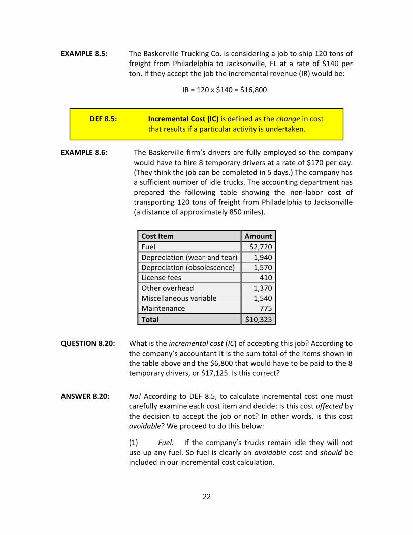
EXAMPLE 8.6: The Baskerville firm’s drivers are fully employed so the company would have to hire 8 temporary drivers at a rate of $170 per day. (They think the job can be completed in 5 days.) The company has a sufficient number of idle trucks. The accounting department has prepared the following table showing the non-labor cost of transporting 120 tons of freight from Philadelphia to Jacksonville (a distance of approximately 850 miles).

Cost Item Amount

Fuel $2,720

Depreciation (wear-and tear) 1,940

Depreciation (obsolescence) 1,570

License fees 410

Other overhead 1,370

Miscellaneous variable 1,540

Maintenance 775

Total $10,325

QUESTION 8.20: What is the incremental cost (IC) of accepting this job? According to the company’s accountant it is the sum total of the items shown in the table above and the $6,800 that would have to be paid to the 8 temporary drivers, or $17,125. Is this correct?

ANSWER 8.20: No! According to DEF 8.5, to calculate incremental cost one must carefully examine each cost item and decide: Is this cost affected by the decision to accept the job or not? In other words, is this cost avoidable? We proceed to do this below:

(1) Fuel. If the company’s trucks remain idle they will not use up any fuel. So fuel is clearly an avoidable cost and should be included in our incremental cost calculation.

DEF 8.5: Incremental Cost (IC) is defined as the change in cost that results if a particular activity is undertaken.

23

(2) Depreciation (wear-and-tear). Presumably the long journey from Philadelphia to Jacksonville will increase the rate at which the company’s trucks are “used up,” hence this item should be included. (The assumption here is that if Baskerville does not accept the job the trucks will remain idle.)

(3) Depreciation (obsolescence). Part of what accountants call depreciation results simply from the passage of time: physical capital goods become obsolete and must be replaced. This will happen whether the trucks are in use or not so this item should not be included.

(4) License fees. Firms must pay license fees of various sorts to all levels of government. These fees would have to be paid whether the job is accepted or not. This item should be excluded.

(5) Other overhead. Overhead is a term used by accountants to indicate costs which are not directly related to the level of production. It is therefore very similar to fixed costs and will not be affected by the decision to accept the job. Overhead costs should be excluded.

(6) Miscellaneous variable costs. The tem “variable” provides the clue. We can automatically assume that it refers to cost items which are related to the amount of transportation services provided by the company, so it clearly should be included as part of incremental cost.

(7) Maintenance. Presumably trucks that were on a long trip need a lot of maintenance but trucks that are idle also require some maintenance. So there is an ambiguity here. If we had more information we could come up with a more definitive answer. But in the absence of such information we will be cautious and assume that this item should be included in our calculation.

What is the Baskerville Company’s incremental cost if they accept this particular job? Given the preceding discussion we have:

IC = $6,800 + $2,720 + $1,940 + $1,540 + $775 = $13,775

QUESTION 8.21: What is the difference between marginal revenue and cost and incremental revenue and cost?

ANSWER 8.21: Here we use the term marginal for small changes (often a one “unit” change) and the term incremental for any change. So if the KLS Corp. is considering building a new plant at a cost of $300

24

million, we say that the incremental cost of this project is $300 million (not small change!)

QUESTION 8.22: Should the Baskerville Trucking Co. accept the job?

ANSWER 8.22: Since the incremental revenue is $16,800 and the incremental cost is $13,775, accepting the job would add $3,025 to the company’s profits, so the job should be accepted, assuming that the company has no reason to expect that a more profitable job may appear over the horizon!

ANSWER 8.22 has an important implication: a decision rule which is at the heart of incremental analysis and is based on the same logic we used in developing the MR = MC rule.

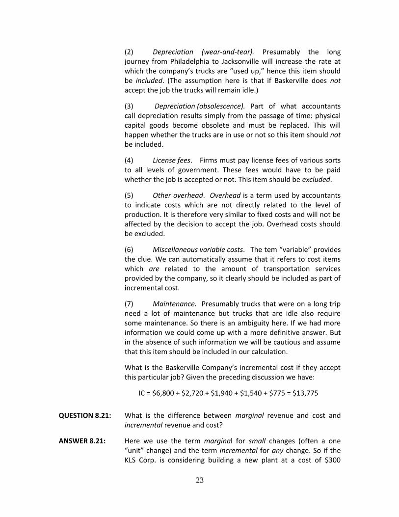
Table 8.5

DECISION RULE 8.4

If: Should I do it?

IR > IC Yes

IR = IC ?

IR < IC No

In Table 8.5 “Should I do it?” means: Should I undertake the particular project I am considering? Should we build the new factory? Should we introduce the new product? And so on. (The question mark in the table means that the decision maker is indifferent: If IR = IC they would be as well off whether they “do it” or not.)

There is a slightly different way to express this decision rule which requires a new definition.

This decision rule is shown in the table below.

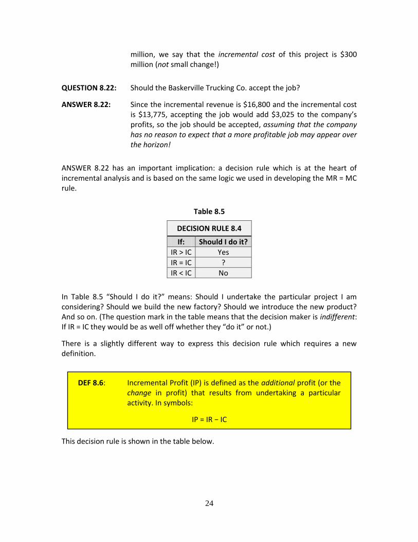
DEF 8.6: Incremental Profit (IP) is defined as the additional profit (or the change in profit) that results from undertaking a particular activity. In symbols:

IP = IR − IC

25

Table 8.6

DECISION RULE 8.4’

If: Should I do it?

IP > 0 Yes

IP = 0 ?

IP< 0 No

DECISION RULES 8.4 and 8.4’ are logically identical and the answer to a decision problem should obviously be the same. So in the case of the Baskerville Trucking Co. we have IR = $16,800, IC = $13,775 so IP = $3,025 > 0 and the answer is the same as before: Accept the job.

NOTE 8.10: There is a close connection between incremental analysis and our earlier discussion of sunk and avoidable costs. REM: sunk costs are unavoidable so they cannot be affected by any particular decision. Therefore they should not be included in any calculation of incremental costs. In fact, the most common error in the application of incremental analysis is the inclusion of sunk costs as part of incremental cost.

26

APPLICATION 8.1

The Plymouth Co.

The Plymouth Co. is a small East Coast Manufacturer of work shirts. The following cost data have been assembled by Margaret Rutherford, Plymouth’s accountant. Monthly overhead is $104,800. The materials that go into each shirt cost $1.70. Labor cost per shirt is $1.65 for skilled labor and $1.10 for unskilled labor. Both kinds of labor are required in the manufacturing process but skilled workers are never required to do unskilled work. Miscellaneous variable costs per shirt come to $0.65. Ms. Rutherford has calculated “fully allocated cost per unit” (equivalent to the economist’s average total cost or ATC) to be $6.41.The standard production volume is 80,000 shirts per month. The usual manufacturer’s price is $7.45 per shirt.

The following additional information may be relevant: The summer months are usually slow and production volume falls to 20,000 shirts per month. In order not to incur extra search and training costs the company keeps its entire skilled work force (but not its unskilled work force) on the payroll in the summer months. If there is not enough work for them to do they engage in training activities and in additional maintenance work. (We assume for simplicity that average variable cost is constant in the relevant range.)

The company receives an order for 50,000 shirts to be produced in July and to be sold under a private label on the West Coast, far from Plymouth’s usual market. The offered price is $4.42 per shirt.

PROBLEM: Should the order be accepted or rejected? (Note: Assume that all the unit costs calculated by Ms. Rutherford are constant over the relevant output range.)

SOLUTION: (1) Calculate Plymouth’s incremental revenue (IR) if the order is accepted:

IR = 50,000 x $4.42 = $221,000

(2) Calculate Plymouth’s incremental cost (IC) if the order is accepted:

27

APPLICATION 8.1, continued

We assume overhead costs to be fixed and should therefore be ignored. The company has a policy of keeping its skilled workers on the payroll in the summer months even if there is not enough work for them to do, which apparently is the case in the summer. So skilled labor is in effect available “for free” and should not be counted as part of incremental cost. Clearly the remaining three cost items are relevant, so we have:

IC = 50,000 x ($1.70 + $1.10 + $0.65) = 50,000 x $3.45 = $172,500 IR = $221,000 > IC = $172,500

The order should be accepted.

(Alternatively, IP = IR − IC = $221,000 − $172,500 = $48,500 > 0 and the order should be accepted.)

APPLICATION 8.2

Globe Air Lines

Globe Air is an expanding regional airline serving mainly the Midwest. The company is committed to flying the Des Moines- Sarasota route three times a week for at least the next two years regardless of economic conditions. They use the Boeing 737, which seats 180 passengers as their standard equipment. Usually 90% of the seats are occupied and based on this “load factor” the accounting department has calculated the cost of flying one passenger one way on this route as shown in the table below.

(1) Labor $17.45

(2) Fuel 8.90

(3) Food Service 5.45

(4) Depreciation 7.25

(5) Other Overhead 14.50

(6) Ground Service 7.90

(7) Maintenance 4.85

Total 66.30

28


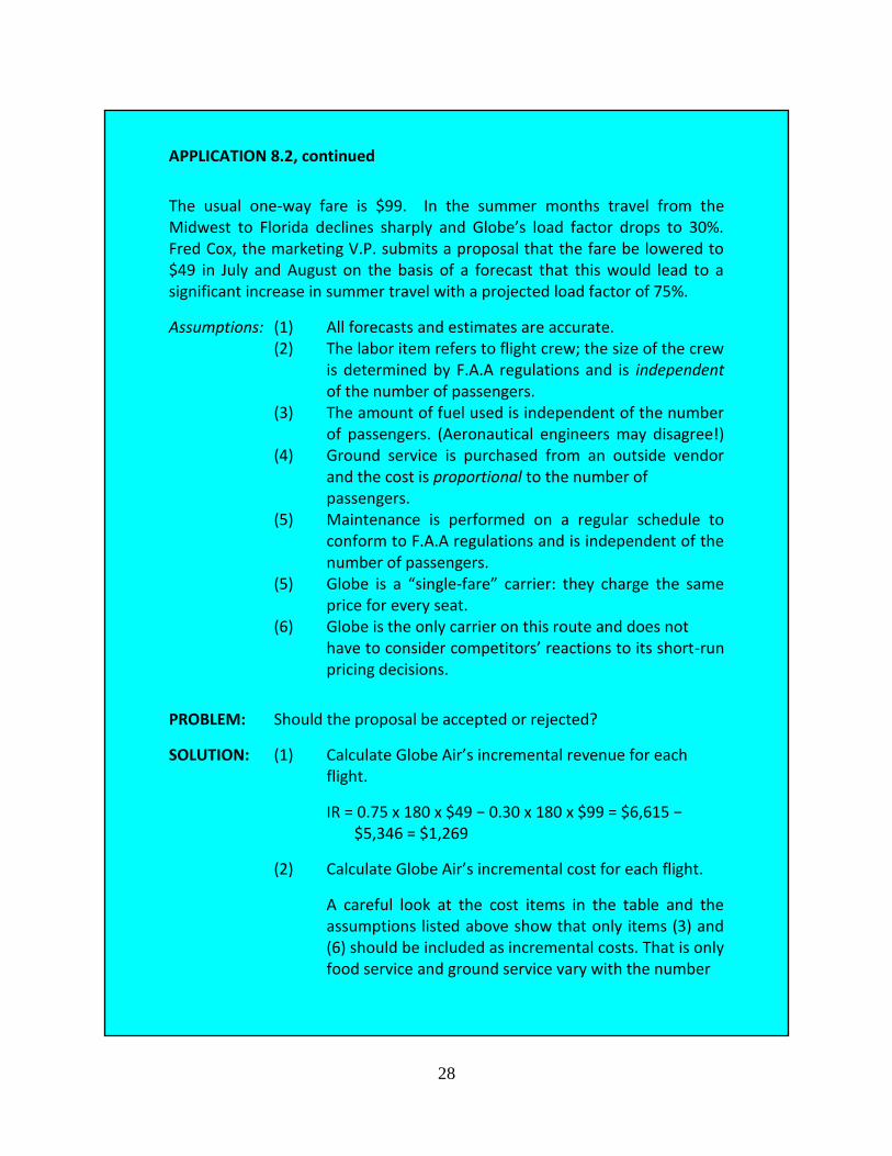
The usual one-way fare is $99. In the summer months travel from the Midwest to Florida declines sharply and Globe’s load factor drops to 30%. Fred Cox, the marketing V.P. submits a proposal that the fare be lowered to $49 in July and August on the basis of a forecast that this would lead to a significant increase in summer travel with a projected load factor of 75%.

Assumptions: (1) All forecasts and estimates are accurate. (2) The labor item refers to flight crew; the size of the crew is determined by F.A.A regulations and is independent of the number of passengers. (3) The amount of fuel used is independent of the number of passengers. (Aeronautical engineers may disagree!) (4) Ground service is purchased from an outside vendor and the cost is proportional to the number of passengers. (5) Maintenance is performed on a regular schedule to conform to F.A.A regulations and is independent of the number of passengers. (5) Globe is a “single-fare” carrier: they charge the same price for every seat. (6) Globe is the only carrier on this route and does not have to consider competitors’ reactions to its short-run pricing decisions.

PROBLEM: Should the proposal be accepted or rejected?

SOLUTION: (1) Calculate Globe Air’s incremental revenue for each flight.

IR = 0.75 x 180 x $49 − 0.30 x 180 x $99 = $6,615 − $5,346 = $1,269

(2) Calculate Globe Air’s incremental cost for each flight.

A careful look at the cost items in the table and the assumptions listed above show that only items (3) and (6) should be included as incremental costs. That is only food service and ground service vary with the number

29

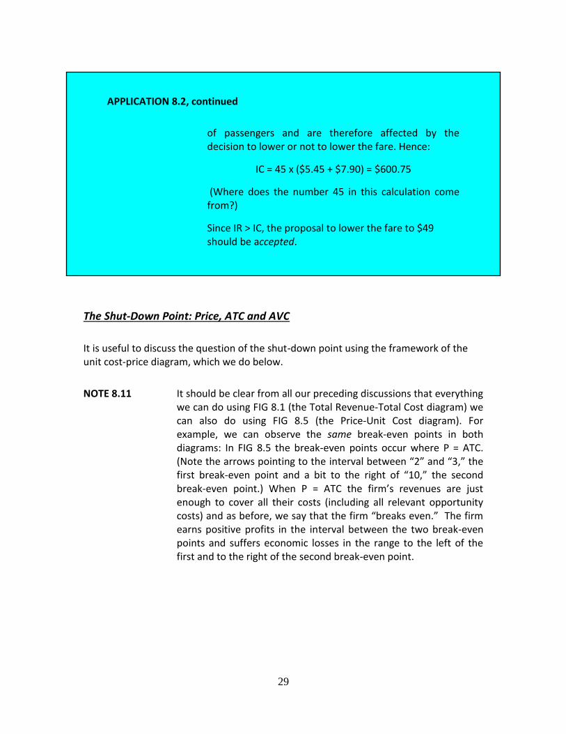
The Shut-Down Point: Price, ATC and AVC

It is useful to discuss the question of the shut-down point using the framework of the unit cost-price diagram, which we do below.

NOTE 8.11 It should be clear from all our preceding discussions that everything we can do using FIG 8.1 (the Total Revenue-Total Cost diagram) we can also do using FIG 8.5 (the Price-Unit Cost diagram). For example, we can observe the same break-even points in both diagrams: In FIG 8.5 the break-even points occur where P = ATC. (Note the arrows pointing to the interval between “2” and “3,” the first break-even point and a bit to the right of “10,” the second break-even point.) When P = ATC the firm’s revenues are just enough to cover all their costs (including all relevant opportunity costs) and as before, we say that the firm “breaks even.” The firm earns positive profits in the interval between the two break-even points and suffers economic losses in the range to the left of the first and to the right of the second break-even point.


of passengers and are therefore affected by the decision to lower or not to lower the fare. Hence:

IC = 45 x ($5.45 + $7.90) = $600.75

(Where does the number 45 in this calculation come from?)

Since IR > IC, the proposal to lower the fare to $49 should be accepted.

30

FIG 8.8

Consider FIG 8.8. It reproduces the unit cost curves from FIG 8.5. It also contains the same demand-marginal revenue “curve” we used previously (with P = $71). Notice the arrow labeled (2) along the vertical axis; it points to the $71 price. This line intersects the MC curve at point b, i.e., an output of 7 and we conclude once again that the profit-maximizing output level for the Brockton Corp. is 7 units. The $71 price line lies above the ATC curve (P > ATC) so we know that TR exceeds TC and Brockton is earning a positive economic profit. But we said in Section 8.1 that since Brockton is a firm in a purely competitive industry the price is determined by “market forces,” i.e., supply and demand. We know that the determinants of supply and demand may change and as a result the market price may change. If the market price increases the demand-MR curve will shift up and Brockton will earn higher profits. But once again interesting questions arise if the market price decreases. (The discussion here will be brief since we covered the essential logic in Section 8.1) We show 3 possibilities:

(1) The price drops to $44. The arrow marked (3) points to the new price line. It is just tangent to the ATC curve; that is, there is a single output level at which P = ATC and the firm breaks even. Since “breaking even” means that they receive a

a

b

c d

e

ATC

AVC

MC

(1)

(5) (4)

(3)

(2)

31

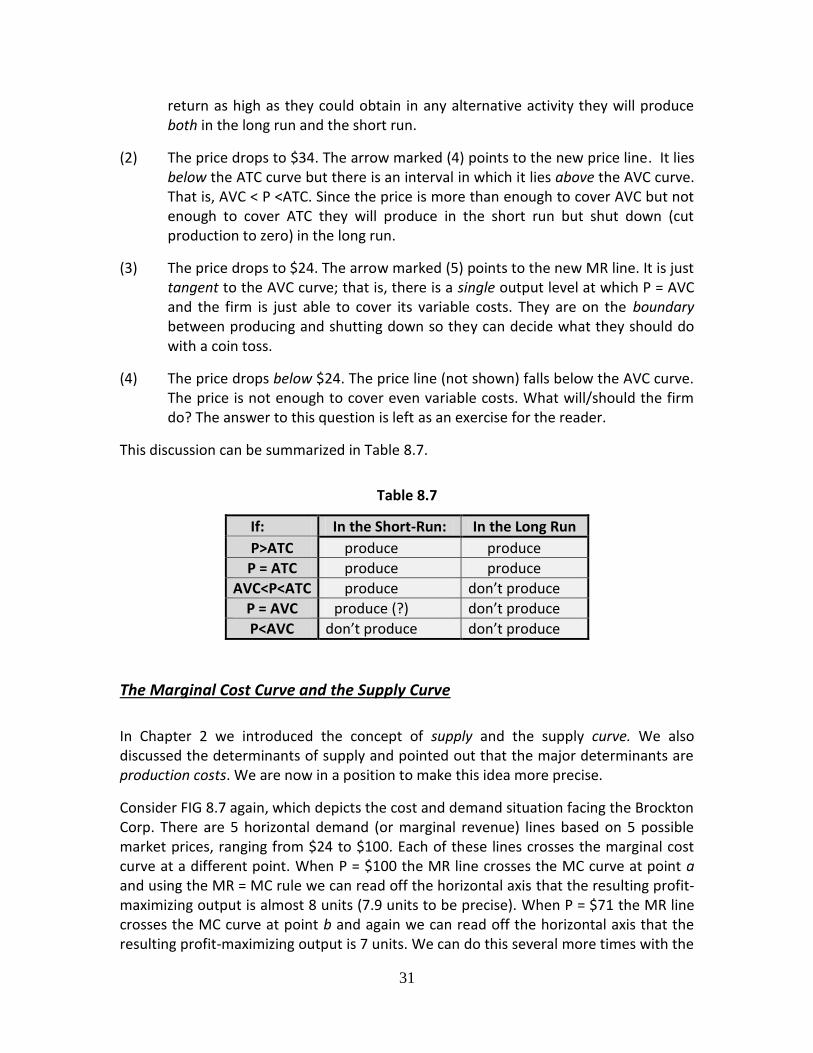
return as high as they could obtain in any alternative activity they will produce both in the long run and the short run.

(2) The price drops to $34. The arrow marked (4) points to the new price line. It lies below the ATC curve but there is an interval in which it lies above the AVC curve. That is, AVC < P <ATC. Since the price is more than enough to cover AVC but not enough to cover ATC they will produce in the short run but shut down (cut production to zero) in the long run.

(3) The price drops to $24. The arrow marked (5) points to the new MR line. It is just tangent to the AVC curve; that is, there is a single output level at which P = AVC and the firm is just able to cover its variable costs. They are on the boundary between producing and shutting down so they can decide what they should do with a coin toss.

(4) The price drops below $24. The price line (not shown) falls below the AVC curve. The price is not enough to cover even variable costs. What will/should the firm do? The answer to this question is left as an exercise for the reader.

This discussion can be summarized in Table 8.7.

Table 8.7

If: In the Short-Run: In the Long Run

P>ATC produce produce

P = ATC produce produce

AVC<P<ATC produce don’t produce

P = AVC produce (?) don’t produce

P<AVC don’t produce don’t produce

The Marginal Cost Curve and the Supply Curve

In Chapter 2 we introduced the concept of supply and the supply curve. We also discussed the determinants of supply and pointed out that the major determinants are production costs. We are now in a position to make this idea more precise.

Consider FIG 8.7 again, which depicts the cost and demand situation facing the Brockton Corp. There are 5 horizontal demand (or marginal revenue) lines based on 5 possible market prices, ranging from $24 to $100. Each of these lines crosses the marginal cost curve at a different point. When P = $100 the MR line crosses the MC curve at point a and using the MR = MC rule we can read off the horizontal axis that the resulting profit-maximizing output is almost 8 units (7.9 units to be precise). When P = $71 the MR line crosses the MC curve at point b and again we can read off the horizontal axis that the resulting profit-maximizing output is 7 units. We can do this several more times with the

32

results shown in the table below. In other words, we have a curve, called the “marginal cost curve” that traces out for us the quantities that the Brockton Corp. is willing and able to supply at different possible market prices, i.e., what we have called the “quantities supplied.”

Price Qs

a $100 7.9

b 71 7.0

c 44 5.6

d 34 5.0

e 24 4.0

QUESTION 8.23: Starting in Chapter 2 what did we call a curve or line that tells us what a firm’s “quantity supplied” is at different possible market prices?

ANSWER 8.23: We called it a supply curve.

NOTE 8.12: It is not entirely correct to say that the firm’s marginal cost curve is its (short-run) supply curve since, as we saw earlier in our discussion of the shutdown point, if the market price is below average variable cost the firm cuts it output to zero. (It “shuts down.”) A more correct statement is made in the following definition:

To get from an individual firm’s supply curve to the market supply curve consider the two panels of FIG 8.9 below.

NOTE 8.13: In the two panels the vertical axes have the same scale but the horizontal axes have different scales. So in Panel B on the horizontal axis one inch might represent one unit but in Panel A it might represent 100 or 1,000 units.

Panel A shows Brockton’s marginal cost curve as wells as their average variable cost curve. The part of the MC curve which lies above the AVC curve (above point m) depicts their supply curve. Assume Brockton is a typical firm in its industry and there are many more like it, with similarly-shaped MC curves. We add these curves “horizontally” and we end up (in Panel B) with the sum of all the MC curves (labeled S = ΣMC), which

DEF 8.7: The portion of a purely competitive firm’s marginal cost curve which lies above the average variable cost curve constitutes the firm’s (short-run) supply curve.

33

constitutes the industry (or market) supply curve. Insert a (market) demand curve which is obtained by adding up all the individual demand curves of potential buyers in this market and we have (in Panel B) the standard market supply-and-demand diagram which we introduced in Chapter 2.

In FIG 8.9(B) the equilibrium price is $100. This price is then “transmitted” to all the individual firms making up this (purely competitive) industry and, since they are price takers, this is the price they will receive (and accept) for their product. So Brockton’s demand curve is drawn at a price of $100 but at this price they can sell any output they decide to produce (and we know, based on the MR = MC rule that at the $100 price they will produce and sell a little less than 8 units.)

FIG 8.9 (A)

Pure Competition in the Long Run

To discuss pure competition from a long run point of view we need new definitions of the short run and the long run from an industry perspective as opposed to an individual firm perspective.

MC = S

AVC

m

P = MR

DEF 8.8: The short run is defined as a period so short that there is not enough time for new firms to enter an industry (or for old firms to exit).

34

FIG 8.9(B)

To enter (or leave) an industry is time-consuming. To enter the garment industry may take months. To enter the electric power industry may take years. But in either case entry (or exit) are not instantaneous. So just like in DEF 5.1 (Chapter 5) “short run “ and “long run” are not calendar concepts but differ across industries depending on a variety of factors such as the industry’s technology, market size, availability of financing, etc.

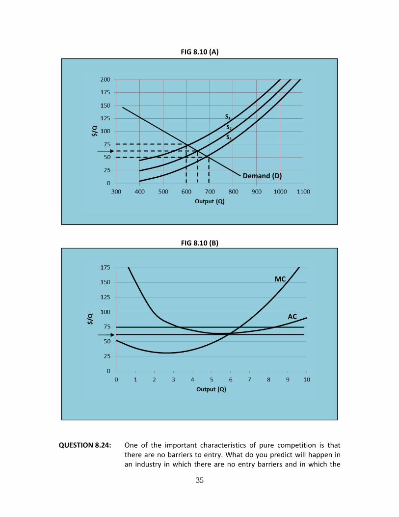
Consider FIG 8.10(A). It is a standard market supply-and-demand diagram. FIG 8.10(B) represents a unit cost and price diagram depicting, once again, the situation of the Brockton Corp, a “typical” firm in this (purely competitive) industry. The average cost curve is labeled AC because for this long-run analysis there is no need to differentiate between fixed and variable costs.

Assume initially that demand is given by D and supply by S1.Then the equilibrium price is

$75. This price is “transmitted” to each firm in the industry. Brockton’s demand-(MR) line lies above its AC line and we conclude that Brockton is earning a “pure” or economic profit.

DEF 8.9: The long run is defined as a period long enough so that there is enough time for new firms to enter an industry (or for old firms to exit).

D

S = ΣMC

35

FIG 8.10 (A)

FIG 8.10 (B)

QUESTION 8.24: One of the important characteristics of pure competition is that there are no barriers to entry. What do you predict will happen in an industry in which there are no entry barriers and in which the

Demand (D)

S1

S2

S3

MC

AC

36

“typical” firm is earning above-normal profits, that is profits higher than they could earn in other industries with similar characteristics?

ANSWER 8.24: Obviously the above-normal profits will attract new firms into the industry. Since “number of producers or sellers” is one of the determinants of supply, supply will increase and the supply curve will shift to the right.

QUESTION 8.25: How long will “entry” continue?

ANSWER 8.25: In principle, as long as there are above-normal profits. (In reality people make mistakes and entry may continue beyond that point.) But sooner or later entry will stop and the above-normal profits will disappear. (We say that they have been “competed away.”) In FIG 8.10 this happens when the supply curve is S2. Then the equilibrium price is approximately $63 (see the arrow in FIG 8.10(B)) and for Brockton and the other firms the horizontal price line is just tangent to their AC curves. The firms in the industry are “breaking even” but we know that this means that they are earning a normal profit.

QUESTION 8.26: We arbitrarily assumed that the initial equilibrium price in the industry is such that the typical firm is earning an above-normal profit. But we could just as easily have started with the assumption that the typical firm is earning a below-normal profit (that is, suffering an economic loss). This is shown in FIG 8.10(A) by D and S3. What do you predict would happen then?


We have arrived at an important point in our discussion which requires us to define a new equilibrium concept called long-run equilibrium.

DEF 8.10: An industry is in long-run equilibrium if there is no tendency for firms either to enter or to leave the industry.

37

Since the typical firm in the industry is breaking even, (i.e., just earning a normal profit) we know that for such a firm P = AC. But more specifically the price line is tangent to the AC curve so we can write P = min AC, that is P = AC at the lowest point of the AC curve. We also know that firms maximize profits when they follow the MR = MC rule and for a firm in a purely competitive industry MR = P. We can therefore define what is called the long-run equilibrium condition for a purely competitive industry as follows:

This is significant because we will show below that when an industry satisfies the condition contained in DEF 8.11 it is “efficient” and in a world of scarcity (REM: Chapter 1) efficiency is a desirable goal to achieve.

Pure Competition and Efficiency

There is an important sense in which pure competition is “efficient” from society’s point of view and therefore serves as a kind of “benchmark” that is used to evaluate other industry types. (REM: Section 8.0)

The following is a rather abstract definition of efficiency as used in economics:

From this perspective there are two types of efficiency: technical and economic or allocative efficiency.

NOTE 8.14: What our previous discussion has revealed is that firms in a purely competitive industry in long-run equilibrium earn just a normal profit (or saying the same thing, zero economic profit).

DEF 8.11: A purely competitive industry is in long-run equilibrium when:

P = MC = min AC

DEF 8.12: A situation is efficient if there is no possible way it can be improved.

38

Technical Efficiency

REM 8.6: In Chapter 1 we discussed the production-possibilities set and its boundary, the production-possibilities frontier (or PPF). Any output bundle in the production-possibilities set but off the PPF represents technical inefficiency because given available resources and technical knowledge more of one good can be produced without producing less of another.

EXAMPLE 8.7: The Terra Co. lays pipe for municipal water and sewage systems. For several years they have employed standard seven-member crews on most of their jobs. Recently they hired a consultant who informed them that current “best-practice” in the industry requires only five-member crews. They responded by reducing the size of their crews accordingly. Before they made the change, Terra was operating in a technically inefficient manner.

COMMENT 8.3: What DEF 8.13 comes down to is that a productive activity is technically efficient if its output is produced at the lowest possible cost given current technology and resource prices.

Firms in purely competitive industries in long-run equilibrium are compelled to be technically efficient. Why?

Consider FIG 8.11 below. It shows the Average Cost curve of a typical firm in a purely competitive industry. We assume that the typical firm engages in “best-practice” production, that is, it is technically efficient. Its AC curve therefore shows the lowest possible unit cost of producing any given level of output. For example, the vertical broken line from “8” on the horizontal axis to point a on the AC curve shows the lowest possible cost of producing 8 units, given current technology and input prices.

DEF 8.13: Technical efficiency (sometimes called production efficiency) exists in any productive activity if: (a) more of one good (good X) cannot be produced without producing less of another (good Y), or (b) the same quantity of a good (good X) cannot be produced by using less of one input (input A) and no more of any other (inputs B, C, D,…).

39

FIG 8.11

REM 8.7: In our discussion of production functions (Chapter 5) and the cost curves derived from them (this chapter) we implicitly assumed that there is technical efficiency in production.

Now assume that there are some firms in the industry that are badly managed. Top managers are lazy and hire their nephews to be in charge of production and marketing. This shows up in Figure 8.11 as an AC curve which lies above the technically-efficient AC curve of the typical firm. It is shown by the broken line marked AC’. In other words, the badly-managed firm has higher unit costs of production than the typical (well-managed) firm.

Assume the industry is not in long-run equilibrium (The market price is $45; note the arrow pointing to “45” along the vertical axis.)

QUESTION 8.27: Can the badly-managed firms survive under these circumstances?

ANSWER 8.27: Yes. As long as the market price in some interval lies above the firm’s AC curve (which presumably includes a normal profit!) the firm is able to survive.

AC

AC’

a

40

QUESTION 8.28: Can the badly-managed firms survive if the industry is in long-run equilibrium?

ANSWER 8.28: In a purely competitive industry in long-run equilibrium P = min AC. “Market forces” drive the price down to the point where the typical firm just “breaks even,” i.e., they earn a normal profit. (This happens in FIG 8.11 when P = $24; note the arrow pointing to “24” along the horizontal axis.) The market price is too low for the badly managed firm to cover all their costs and they are unable to survive.

Allocative Efficiency

We have said several times in previous chapters, starting in Chapter 1, that we live in a world of scarcity. Hence a central theme in economics is the desirability of an “efficient” or “proper” or “optimal” allocation of resources. Scarce productive resources are allocated efficiently over different goods, activities or actions from a social point of view if the allocation conforms to the preferences of the individuals making up the society. We start the discussion with the following abstract definition of allocative efficiency:

NOTE 8.15: An obvious addition to DEF 8.14 is that if a situation exists in which at least one individual can be made better off without making anyone worse off the situation is not allocatively efficient.

One of the three major problems confronting every economic system is to decide what to produce (REM: Chapter 1). We now ask: Is this decision made in a way which is allocatively efficient or not?

EXAMPLE 8.8: Coruna is an island nation in the Mediterranean. Its people prefer black shoes but its economy is run in such a way that warehouses are full of brown shoes that no one wants. Coruna’s economy is not allocatively efficient. A reallocation of productive resources from

CONCLUSION 8.1: Firms in purely competitive industries in long-run equilibrium are compelled to be technically efficient.

DEF 8.14: A situation is allocatively efficient if no individual can be made better off without making any one else worse off.

41

brown shoes to black shoes would increase the well-being of the people of Coruna.

FIG 8.12

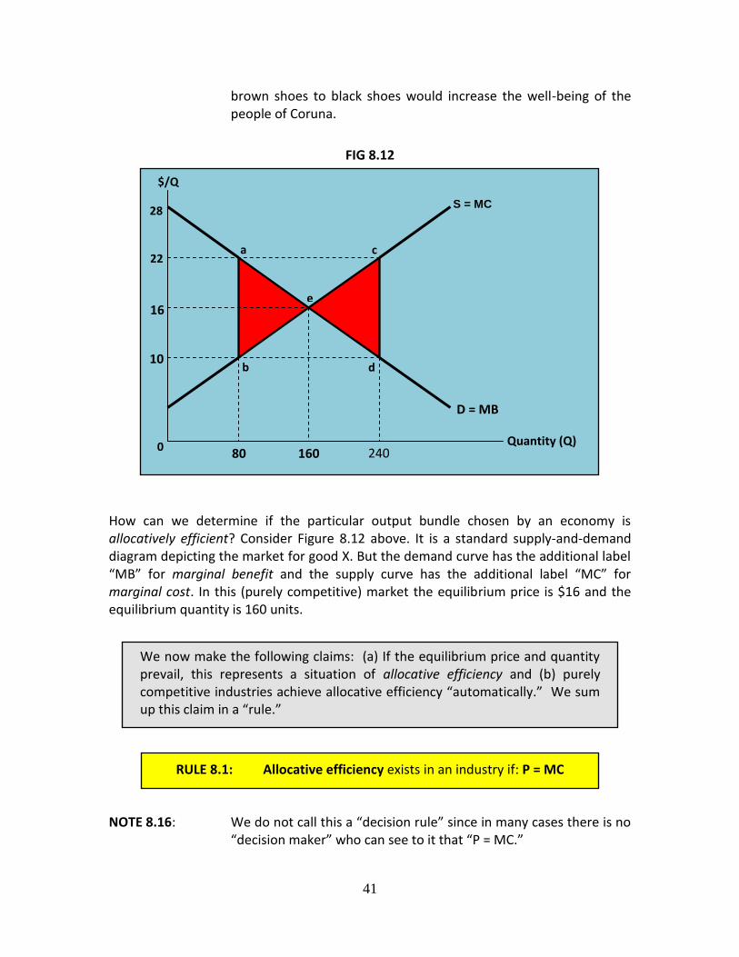
How can we determine if the particular output bundle chosen by an economy is allocatively efficient? Consider Figure 8.12 above. It is a standard supply-and-demand diagram depicting the market for good X. But the demand curve has the additional label “MB” for marginal benefit and the supply curve has the additional label “MC” for marginal cost. In this (purely competitive) market the equilibrium price is $16 and the equilibrium quantity is 160 units.

NOTE 8.16: We do not call this a “decision rule” since in many cases there is no “decision maker” who can see to it that “P = MC.”

RULE 8.1: Allocative efficiency exists in an industry if: P = MC

We now make the following claims: (a) If the equilibrium price and quantity prevail, this represents a situation of allocative efficiency and (b) purely competitive industries achieve allocative efficiency “automatically.” We sum up this claim in a “rule.”

0 80 160 240

D = MB

S = MC

10

16

22

28

a c

b d

$/Q

e

Quantity (Q)

42

NOTE 8.17: There are situations, which we will discuss in later chapters, especially in Chapter 12, where a decision-maker (for example a regulatory agency) is able to influence the price of a good or service in such a way that the end result may be P= MC. If such a pricing rule is followed it is called marginal-cost pricing.

Why is an industry allocatively efficient if P = MC?

REM 8.8: In Chapter 2 we pointed out that a demand curve can also be thought of as a “marginal benefit” or “willingness-to-pay” curve. Why? In FIG 8.12 we can read off the demand curve that at a price of a bit less than $28 (say $27.97) there is one individual who would buy one unit of this good. Why is this individual willing to pay this price? Presumably because that is what good X is “worth” to him: it is the “marginal benefit” he receives (or expects to receive) from one unit of the good. Assume for simplicity that each individual in this market buys just one unit. Then there is a second individual who is willing to pay a bit less than the first (say $27.94) for one unit. We ask the same question again and come up with the same answer: The second individual is willing to pay the $27.94 price because that is what good X is worth to her. The price she is willing to pay represents her evaluation of the (marginal) benefit she receives (or expects to receive) from this good. We proceed in the same way until we reach the 160th individual: Given the $16 equilibrium price she is just on the boundary between buying and not buying. Assume that she buys. Then we can say that the marginal benefit of good X for the 160 individuals who buy the good at the $16 equilibrium price is at least $16. And since for any quantity shown on the horizontal axis we can read off the curve what the marginal benefit obtained by the “last” buyer is, we can also think of the demand curve as representing a “marginal benefit” curve.

REM 8.9 In this chapter we discovered that the market supply curve is constructed by adding up the marginal cost curves of the individual firms making up the industry. So if we pick an arbitrary quantity on the horizontal axis in FIG 8.12 we can read off the supply curve what the corresponding marginal cost is. For example, the MC of the 240th unit of good X is $22. (Can you see why?) But “cost” in economics means opportunity cost. So when we say that the MC of the 240th unit is $22 we mean that the highest-valued alternative good that could be produced with the same bundle of resources is worth $22 to someone in this society.

43

So according to the claim we are making, the market depicted in FIG 8.12 is allocatively efficient if the price charged is $16 and the quantity bought and sold is 160 units. But why?

Assume that the market for good X is interfered with in some way: A government agency insists that a price higher (or lower) than $16 be charged; a monopoly takes over the industry, or whatever.

QUESTION 8.29: Say the price ends up at P = $22 and people buy 80 units of god X. Why does this represent a situation of allocative inefficiency, or expressed differently, a misallocation of resources?

ANSWER 8.29: Again, think in marginal terms. Would “society” be better off if 81 units of good X were produced instead of 80? The answer is yes, since the value of the 81st unit (the marginal benefit, or MB) to someone in this society is a bit less than $22 whereas the value of the alternative good that could be produced with the same bundle of resources (the marginal cost, or MC) is a bit more than $10. So switching resources from elsewhere in the economy to producing an additional unit of good X would create a net benefit of a bit less than $12. Would society be better off if 82 units of good X were produced instead of 81? The answer is again yes. We continue along this line until we reach an output of 160 units. We now ask again: Would society be better off if 161 units were produced instead of 160? The answer is no since the MB of the 161st unit is a bit less than $16 while the MC is a bit more than $16, so there is a small net loss from producing the 161st unit. So as long as MB > MC there is a net gain to society if production is increased and as long as MB < MC there is a net gain to society if production is reduced. We conclude that when MB = MC the “optimal” quantity is produced (from society’s point of view). It represents a situation of allocative efficiency. But MB is identical to price and so we end up with the P = MC rule.

QUESTION 8.30: What is the cost to society of underproducing good X, for example by producing 80 units instead of 160 units?

ANSWER 8.30: The cost is shown by the area of the triangle bae shown in red. A bit of elementary geometry reveals that this amounts to $480.

QUESTION 8.31: What is the cost to society of overproducing good X, for example by producing 240 units instead of 160 units?


44

QUESTION 8.32: How does the P= MC rule relate to DEF 8.14 and its addition (If a situation exists in which at least one individual can be made better off without making anyone worse off the situation is not allocatively efficient)?

ANSWER 8.32: Consider FIG 8.12 again. Assume that 80 units of good X are being produced. The fact that MB > MC constitutes a signal: There are some people in this society who would prefer that more of good X be produced rather than its highest-valued alternative, good Y. They go to those who are currently consuming good Y and they make an offer: Allow us to reallocate some of the resources from their current activity (producing good Y) to producing a little more (say one unit more) of good X. We will pay you $16 for those resources. (The amount has to lie somewhere between $16 and $22. Can you see why?) An agreement is reached and the transfer of resources takes place. Both sides benefit and no one is hurt. Why? Because the people who prefer good X were willing to pay a little bit less than$22 for an additional unit, yet they got it for $16. The people who prefer good Y value the unit they “gave up” at a bit over $10, yet they got $16. (They would rather have $16 than a unit of good Y.) Both parties benefited from the bargain and no one was hurt, so the initial situation could not have been allocatively efficient.

NOTE 8.18: It is important to understand that we are not making the claim that a purely competitive industry is always and everywhere allocatively efficient. There are numerous instances, called market failures, which we will discuss in several places, especially in Chapter X in which a purely competitive industry simply fails to “register” all the costs and/ or benefits associated with a productive activity and therefore may underproduce (or overproduce) a good or service when viewed from a social point of view, even though the P = MC condition is satisfied.

NOTE 8.19: Because of our conclusion that a purely competitive industry in long-run equilibrium is both technically and allocatively efficient we shall use it as a “benchmark” to evaluate other industry types in subsequent chapters.

45

PROBLEMS:

Q TFC TVC TC AFC AVC ATC MC

0 --- --- --- ---

1 17

2 34

3 14

4 9 10

5 100

6 85

7 151

8 20

9 56

(1) Consider the table above. It describes the cost structure of the Jericho Co., a single-product firm in a purely competitive industry. (Assume that only “whole” units can be produced; i.e., 3 units but not 3.4 units.)

(a) Fill in all the blank cells. (b) If the market price is $37, what is Jericho’s profit-

maximizing output (Q*) in the long run? The short-run? (c) Calculate Jericho’s profit at Q*, Q* − 1 and Q* + 1. Do the

results of these calculations support the MR (=P) = MC rule? Explain.

(d) If the market price drops to $17, what is Jericho’s profit-maximizing output in the long run? The short-run? Explain.

(e) If the market price drops to $11, what is Jericho’s profit-maximizing output in the long run? The short-run? Explain.

(2) Consider the diagram below. It represents the cost situation of the Ramsey Co., a small metal-grinding firm located in Pittsburgh. Ramsey’s management view all their costs as variable, hence no distinction is made between average variable and average total cost. Assume the industry is purely competitive.

(a) If the market price is $30, what is Ramsey’s profit-maximizing output (Q*)?

46

0

10

20

30

40

0 40 80 120 160 200 240 280

Quantity (Q)

$/Q

AC

MC

(b) At Q* what is Ramsey’s total revenue (TR), total cost (TC), and total profit (Π)?

(c) If the market price is $20, what is Ramsey’s profit-maximizing output (Q**)? At Q** what is TR, TC and Π?

(d) Construct a table showing Ramsey profit-maximizing output at market prices ranging from 0 to $40 at $5 intervals (i.e., $5, $10,…).

(e) Explain why the resulting table represents Ramsey’s supply schedule.

(3) Mollyplast, Inc. is a medium-size manufacturer of plastic cups and similar commodities produced by injection molding. Their “normal” output is 275,000 gross per month. They have a relatively steady customer base on the East coast but in recent months their market has “softened” and they are experiencing excess capacity: their output has shrunk to 200,000 gross per month. The usual price for the cups is $5.45 per gross. They have recently received an order from a supermarket chain located in the Midwest for 70,000 gross of this product but the offered price is $4.65. Jim Dine, Mollyplast’s CEO, must decide whether to accept or reject the order. The table below shows the accounting department’s estimate of the firm’s costs, calculated at a normal output level, i.e., at Q = 275,000. [Assume average variable costs and their components are constant throughout.]

47

Total Per Unit

Materials $290,000 $1.05

Direct Labor 715,000 2.60

Administrative and sales 88,000 0.32

Utilities 17,000 0.06

Other variable costs 151,000 0.55

Other fixed costs 34,000 0.12

Total $1,295,000 $4.71

Should the order be accepted or rejected? Explain, using incremental analysis.

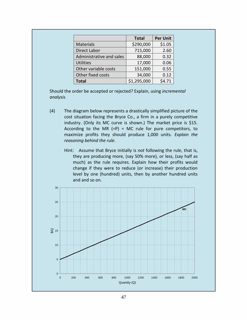
(4) The diagram below represents a drastically simplified picture of the cost situation facing the Bryce Co., a firm in a purely competitive industry. (Only its MC curve is shown.) The market price is $15. According to the MR (=P) = MC rule for pure competitors, to maximize profits they should produce 1,000 units. Explain the reasoning behind the rule.

Hint: Assume that Bryce initially is not following the rule, that is, they are producing more, (say 50% more), or less, (say half as much) as the rule requires. Explain how their profits would change if they were to reduce (or increase) their production level by one (hundred) units, then by another hundred units and and so on.

0

5

10

15

20

25

30

0 200 400 600 800 1000 1200 1400 1600 1800 2000

Quantity (Q)

$/Q

MC

48

(5) Horn of Plenty is a large buffet-style restaurant located on the New Jersey shore, a popular summer resort area on the East coast. They offer dinners at a single price of $29. Their dining room and kitchen can accommodate 10,000 diners a week and during the summer months they usually serve that number. In the fall they suffer a sharp drop in patronage serving only about 2,000 customers a week. The restaurant’s practice has been to maintain the $29 price during the slow fall season. John Dean, the Assistant Manger, has approached the owners with a proposal to lower the price in the fall to $19.95. He estimates that this would increase patronage to 9,000 per week.

The restaurant’s accountant has prepared the following cost estimates, based on the assumption that 10,000 meals per week are being served

Total Per meal

Food $44,500 $4.45

Labor 67,500 6.75

Management and supervision 19,500 1.95

Other variable costs 41,500 4.15

Other fixed costs 28,500 2.85

Total 201,500 20.15

Make the following additional assumptions:

Dean’s estimates are reliable. Managers are kept on the payroll throughout the year. Average variable cost and its component are constant

throughout.

Should the price be lowered in the fall or not? Explain, using incremental analysis.

49

(6) Consider the graph below. It shows the cost situation facing the Rutherford Co., a purely competitive producer of widgets. (Assume that Rutherford is a “typical” firm in the widget industry.) For the purpose of this question there is no need to differentiate between average total and average variable costs so we just use the label “AC.” The current market price of widgets is $145.

(a) What is Rutherford’s profit-maximizing output? (b) Is the Rutherford Co. earning a “pure” (or “economic” or

“above-normal”) profit or just a normal profit? Explain. (c) Is the widget industry in long-run equilibrium? Explain. (d) If not, what is the industry’s long-run equilibrium price?

What would be Rutherford’s output at that price? Explain. (e) Describe the process by which the widget industry would

move toward long-run equilibrium if it is not there already.

135

140

145

150

155

160

0 2 4 6 8 10 12 14 16

Quantity (Q)

$/Q

MC

AC

chapter 8 pure competition -...

Documents