chapter 9
DESCRIPTION
Chapter 9. Gas Power Systems. Learning Outcomes. Perform air-standard analyses of internal combustion engines based on the Otto, Diesel, and dual cycles, including: sketching p - v and T - s diagrams and evaluating property data at principal states. - PowerPoint PPT PresentationTRANSCRIPT

Chapter 9
Gas Power Systems

Learning Outcomes
►Perform air-standard analyses of internal combustion engines based on the Otto, Diesel, and dual cycles, including:►sketching p-v and T-s diagrams and evaluating
property data at principal states.►applying energy, entropy, and exergy
balances.►determining net power output, thermal
efficiency, and mean effective pressure.

Learning Outcomes
►Perform air-standard analyses of gas turbine power plants based on the Brayton cycle and its modifications, including:►sketching T-s diagrams and evaluating
property data at principal states.►applying mass, energy, entropy, and exergy
balances.►determining net power output, thermal
efficiency, back work ratio, and the effects of compressor pressure ratio.
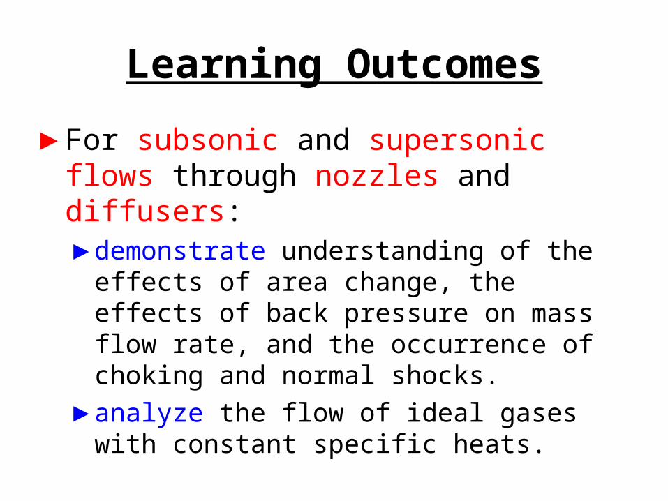
Learning Outcomes
►For subsonic and supersonic flows through nozzles and diffusers:►demonstrate understanding of the effects of
area change, the effects of back pressure on mass flow rate, and the occurrence of choking and normal shocks.
►analyze the flow of ideal gases with constant specific heats.

Considering Compressible Flow► In many applications of engineering interest, gases move at relatively high speeds and exhibit significant changes in specific volume (density). They include
►Flows through the nozzles and diffusers of jet engines.►Flows through wind tunnels, shock tubes, and steam ejectors.
These flows are known as compressible flows.
► Next, we consider some important preliminaries, including the
►momentum equation for steady one-dimensional flow►velocity of sound and Mach number►stagnation state
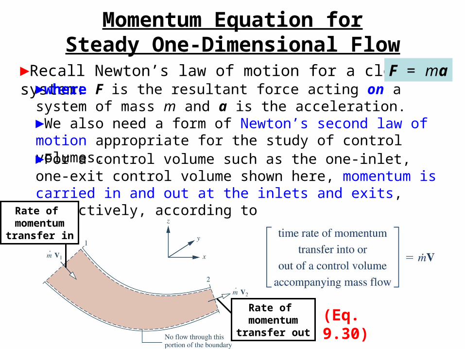
Momentum Equation forSteady One-Dimensional Flow
►Recall Newton’s law of motion for a closed system: F = ma►where F is the resultant force acting on a system of mass m and a is the acceleration.►We also need a form of Newton’s second law of motion appropriate for the study of control volumes.
(Eq. 9.30)
►For a control volume such as the one-inlet, one-exit control volume shown here, momentum is carried in and out at the inlets and exits, respectively, according to
Rate of momentumtransfer in
Rate of momentumtransfer out

net rate at which momentum is transferred into the control
volume accompanying mass flow
Momentum Equation forSteady One-Dimensional Flow
►In words, Newton’s second law for a control volume is:
time rate of changeof momentum contained within the control volume
resultant forceacting on the
control volume= +
(= 0 at steady state)
►The form of the momentum equation for a one-inlet, one-exit control volume at steady state is:
(Eq. 9.31)

Velocity of Sound
► Analyses using mass and momentum equations supported by experimental data reveal that the relation between pressure and specific volume across a sound wave is nearly isentropic, and that its velocity c – called the velocity of sound – is given by
(Eq. 9.36b)
► A sound wave is a small pressure disturbance that propagates through a gas, liquid, or solid at a velocity c that depends on the properties of the medium.

Velocity of Sound►The special case of an ideal gas with constant specific heats is used extensively in Chapter 9. For this case, the relationship between pressure and specific volume for fixed entropy is pvk = constant where k is the specific heat ratio. Using this relationship, Eq. 9.36b becomes
(Eq. 9.37)
► The velocity of sound is an intensive property whose value depends on the state of the medium through which sound propagates. While sound propagates nearly isentropically, the medium itself may be undergoing any process.

Velocity of Sound
Example: Calculate the velocity of sound in air at 300 K and 650 K.
►From Table A-20 at 300 K, k = 1.4. Thus from Eq. 9.37
N 1
m/skg 1K) 300(
Kkg
mN
97.28
83144.1
2
c = 347 m/s (1138 ft/s)
►From Table A-20 at 650 K, k = 1.37. Thus from Eq. 9.37
N 1
m/skg 1K) 650(
Kkg
mN
97.28
831437.1
2
c = 506 m/s (1660 ft/s)

Mach Number►In subsequent discussions, the ratio of velocity V at a state in a flowing fluid to the value of sonic velocity c at the same state plays an important role. This ratio is called the Mach number, M.
(Eq. 9.38)
► Several important terms associated with Mach number are shown in the table.
Mac h Number T erm
M < 1 S ubs onic
M = 1 S onic
M > 1 S upers onic
M >> 1 Hypers onic
M near 1 T rans onic
Mac h Number T erm
M < 1 S ubs onic
M = 1 S onic
M > 1 S upers onic
M >> 1 Hypers onic
M near 1 T rans onic

Actual compressibleflow process
h
h
s
p
V
ho
po
Vo = 0
Actual compressibleflow process
h
h
s
p
V
ho
po
Vo = 0
Stagnation State Properties
►The h-s diagram shows a compressible flow process.Associated with each state of the flow is a reference state known as the stagnation state.►The stagnation state is the state the flowing gas would attain if it were decelerated to zero velocity isentropically. ►By reducing an energy balance for a hypothetical diffuser that – in principle only – decelerates the gas, we get
(Eq. 9.39)
Stagnation state:ho = stagnation enthalpy, po = stagnation pressure, To = stagnation temperature
One-Dimensional Steady Flowin Nozzles and Diffusers
► Owing to important applications for nozzles and diffusers, the remainder of our study of compressible flow centers on them.►We begin by establishing criteria for determining whether a nozzle or diffuser should have a converging, diverging, or converging-diverging shape.►These criteria are determined from differential equations obtained in Sec.9.13.1 using isentropic property relations. Since actual flows through well-designed nozzles and diffusers are nearly isentropic (Sec. 6.12.2), findings drawn from the differential equations are observed for such flows as well.

One-Dimensional Steady Flowin Nozzles and Diffusers
►One of these equations relates velocity and pressure changes in the direction of flow:
(Eq. 9.44)
►When velocity increases: dV > 0, then pressure decreases: dp < 0.►When velocity decreases: dV < 0, then pressure increases: dp > 0.

One-Dimensional Steady Flowin Nozzles and Diffusers
►Another equation relates velocity and area changes in the direction of flow:
(Eq. 9.45)
►There are four cases, each of which depends on the local Mach number M:
►Subsonic nozzle: dV > 0 and M < 1 → dA < 0. The duct converges.
Subsonic NozzleVelocity increasesArea decreases
Pressure decreases

One-Dimensional Steady Flowin Nozzles and Diffusers
►Another equation relates velocity and area changes in the direction of flow:
(Eq. 9.45)
►There are four cases, each of which depends on the local Mach number M:
►Supersonic nozzle: dV > 0 and M > 1 → dA > 0. The duct diverges.
Supersonic NozzleVelocity increases
Area increasesPressure decreases

One-Dimensional Steady Flowin Nozzles and Diffusers
►Another equation relates velocity and area changes in the direction of flow:
(Eq. 9.45)
►There are four cases, each of which depends on the local Mach number M:
►Supersonic diffuser: dV < 0 and M > 1 → dA < 0. The duct converges.
Supersonic DiffuserVelocity decreases
Area decreasesPressure increases

One-Dimensional Steady Flowin Nozzles and Diffusers
►Another equation relates velocity and area changes in the direction of flow:
(Eq. 9.45)
►There are four cases, each of which depends on the local Mach number M:
►Subsonic diffuser: dV < 0 and M < 1 → dA > 0. The duct diverges.
Subsonic DiffuserVelocity decreases
Area increasesPressure increases

Exploring the Effects of Area Changein Subsonic and Supersonic Flows
►Consider a converging section with subsonic flow connected to a diverging section to form a converging-diverging duct.►If the Mach number is unity at the end of the converging section, and the flow continues to accelerate, the flow will become supersonic in the diverging section.
M = 1 at the throat. This is called a converging-diverging nozzle.
Velocity increases, pressure decreases
Exploring the Effects of Area Changein Subsonic and Supersonic Flows
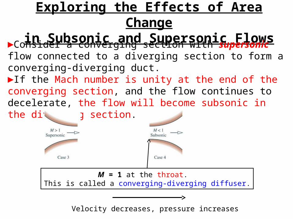
►Consider a converging section with supersonic flow connected to a diverging section to form a converging-diverging duct.►If the Mach number is unity at the end of the converging section, and the flow continues to decelerate, the flow will become subsonic in the diverging section.
M = 1 at the throat. This is called a converging-diverging diffuser.
Velocity decreases, pressure increases

Exploring the Effects of Area Changein Subsonic and Supersonic Flows
►These findings indicate that a Mach number of unity can occur only at the location in a nozzle or diffuser where the flow area is a minimum. This location of minimum area is called the throat.►As shown in the following discussion, a Mach number of unity does not necessarily occur at the location where flow area is a minimum.

Effects of Back Pressure on Mass Flow Rate – Converging Nozzle
►Consider a converging duct with stagnation conditions at the inlet, discharging into a region outside the nozzle where the pressure pB – called the back pressure – can be varied.►We explore how the mass flow rate through the nozzle and the pressure at the nozzle exit vary as the back pressure is decreased while keeping the nozzle inlet conditions fixed.

Effects of Back Pressure on Mass Flow Rate – Converging Nozzle
Case a. When pB = pE = po, there is no flow: .0m

Effects of Back Pressure on Mass Flow Rate – Converging Nozzle
Case a. When pB = pE = po, there is no flow: .0mCases b and c. As pB is decreased, the mass flow rate increases, flow is subsonic throughout. The pressure at the nozzle exit equals the back pressure.

Effects of Back Pressure on Mass Flow Rate – Converging Nozzle
Case a. When pB = pE = po, there is no flow: .0mCases b and c. As pB is decreased, the mass flow rate increases, flow is subsonic throughout. The pressure at the nozzle exit equals the back pressure.Case d. Eventually, as pB is decreased, a Mach number of unity is attained at the nozzle exit. The corresponding exit pressure is called the critical pressure, denoted by p*. The mass flow rate is the maximum possible and the nozzle is said to be choked.
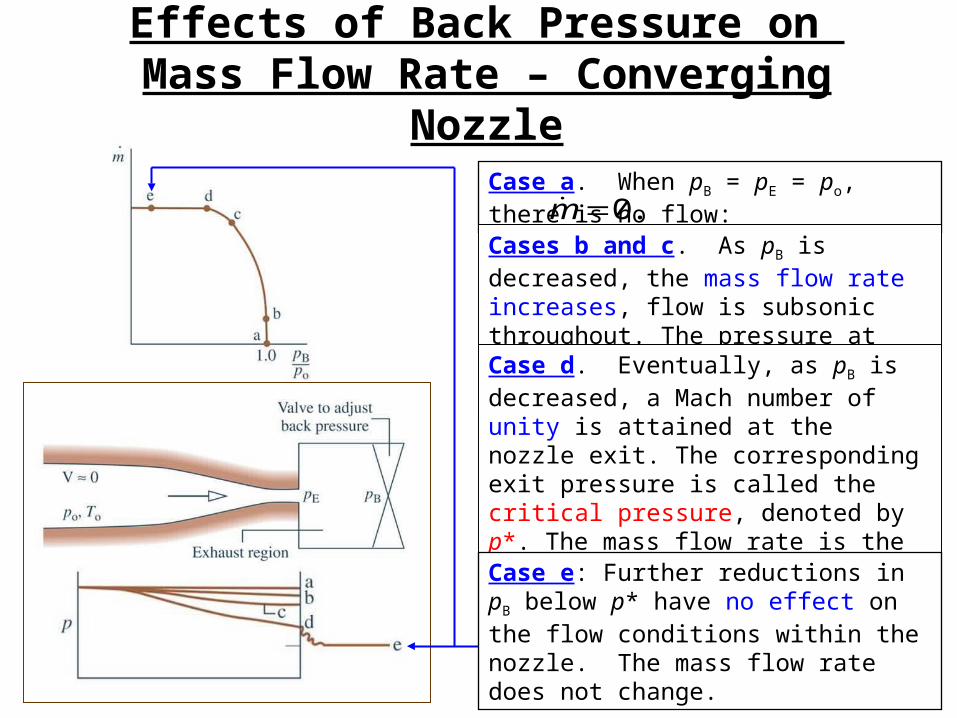
Effects of Back Pressure on Mass Flow Rate – Converging Nozzle
Case a. When pB = pE = po, there is no flow: .0mCases b and c. As pB is decreased, the mass flow rate increases, flow is subsonic throughout. The pressure at the nozzle exit equals the back pressure.Case d. Eventually, as pB is decreased, a Mach number of unity is attained at the nozzle exit. The corresponding exit pressure is called the critical pressure, denoted by p*. The mass flow rate is the maximum possible and the nozzle is said to be choked. Case e: Further reductions in pB below p* have no effect on the flow conditions within the nozzle. The mass flow rate does not change.
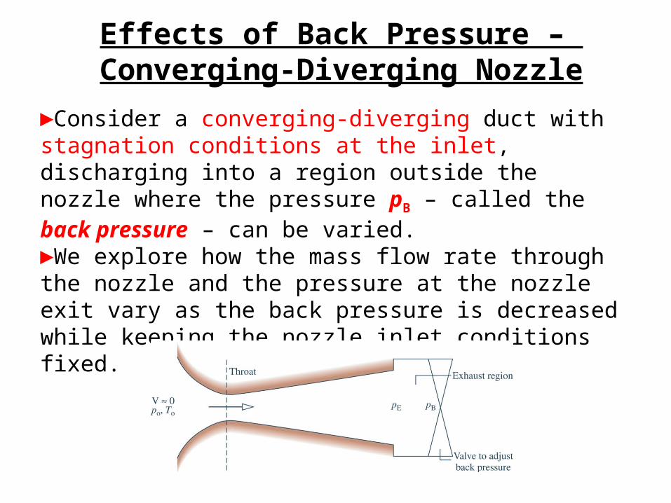
Effects of Back Pressure – Converging-Diverging Nozzle
►Consider a converging-diverging duct with stagnation conditions at the inlet, discharging into a region outside the nozzle where the pressure pB – called the back pressure – can be varied.►We explore how the mass flow rate through the nozzle and the pressure at the nozzle exit vary as the back pressure is decreased while keeping the nozzle inlet conditions fixed.
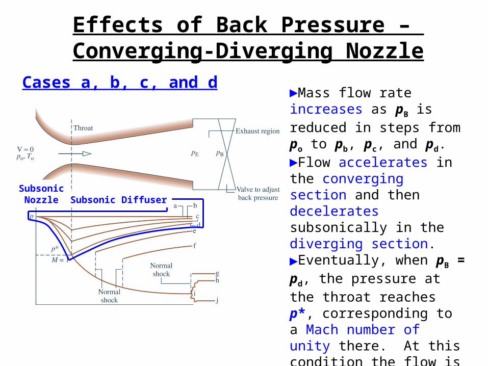
Effects of Back Pressure – Converging-Diverging Nozzle
►Mass flow rate increases as pB is reduced in steps from po to pb, pc, and pd.►Flow accelerates in the converging section and then decelerates subsonically in the diverging section.►Eventually, when pB = pd, the pressure at the throat reaches p*, corresponding to a Mach number of unity there. At this condition the flow is choked, and mass flow rate cannot increase with further decrease in back pressure.
Cases a, b, c, and d
SubsonicNozzle Subsonic Diffuser
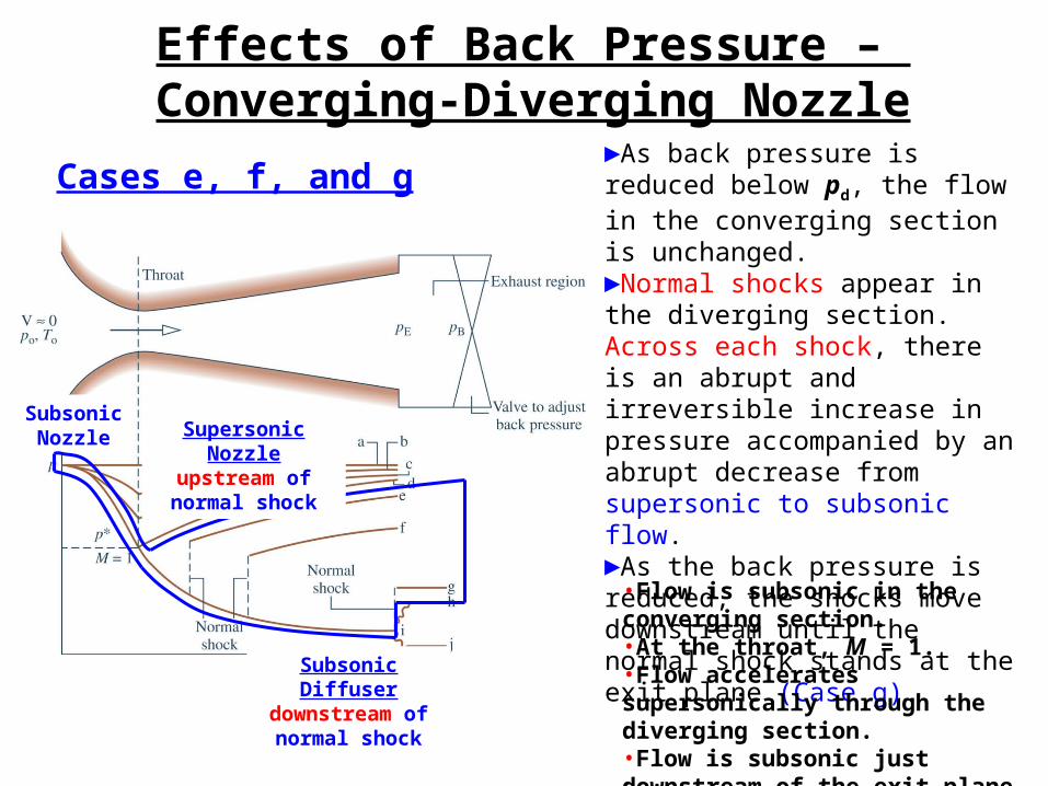
Effects of Back Pressure – Converging-Diverging Nozzle
►As back pressure is reduced below pd, the flow in the converging section is unchanged.►Normal shocks appear in the diverging section. Across each shock, there is an abrupt and irreversible increase in pressure accompanied by an abrupt decrease from supersonic to subsonic flow.►As the back pressure is reduced, the shocks move downstream until the normal shock stands at the exit plane (Case g).
Cases e, f, and g
SubsonicNozzle
Subsonic Diffuserdownstream of normal shock
Supersonic Nozzleupstream of
normal shock
•Flow is subsonic in the converging section.•At the throat, M = 1.•Flow accelerates supersonically through the diverging section.•Flow is subsonic just downstream of the exit plane.

Effects of Back Pressure – Converging-Diverging Nozzle
►Back pressure is less than that of Case g.►Flow in the nozzle is not affected; adjustment occurs outside the nozzle.►Case h: Pressure increase outside the nozzle involves an oblique compression shock.
Cases h, i, and j
SubsonicNozzle Supersonic Nozzle

Effects of Back Pressure – Converging-Diverging Nozzle
►Back pressure is less than that of Case g.►Flow in the nozzle is not affected; adjustment occurs outside the nozzle.►Case h: Pressure increase outside the nozzle involves an oblique compression shock.►Case i: Unique back pressure for which no shocks occur within or outside nozzle.
Cases h, i, and j
SubsonicNozzle Supersonic Nozzle

Effects of Back Pressure – Converging-Diverging Nozzle
►Back pressure is less than that of Case g.►Flow in the nozzle is not affected; adjustment occurs outside the nozzle.►Case h: Pressure increase outside the nozzle involves an oblique compression shock.►Case i: Unique back pressure for which no shocks occur within or outside nozzle.►Case j: The gas expands outside the nozzle through an oblique expansion wave.
Cases h, i, and j
SubsonicNozzle Supersonic Nozzle

Modeling Normal Shocks
►Depending on the back pressure, a normal shock can stand in the diverging section of a supersonic nozzle, as shown in the figure
where the subscripts x and y denote, respectively, the states just upstream and downstream of the shock.
►Since the thickness of the shock is small, there is no appreciable change in flow area across the shock and the only significant forces acting on the control volume in the direction of flow are the pressure forces. Additionally, for the control volume .0cv Q

Modeling Normal Shocks►At steady state, mass, energy, momentum, and entropy balances reduce to give the following relations between the upstream, x, and downstream, y, locations.
Mass: (Eq. 9.46)
Energy: (Eq. 9.47a)
Momentum: (Eq. 9.48)
Entropy: (Eq. 9.49)
Since the shock is an irreversibility, the entropy balance requires that the downstream specific entropy sy is greater than the upstream specific entropy sx.

Modeling Normal Shocks
►The mass and energy equations together with property data for the particular gas combine to give a curve on an h-s diagram called a Fanno line.
Mass:
Energy:

Modeling Normal Shocks
►The mass and momentum equations together with property data for the particular gas combine to give a curve on an h-s diagram called a Rayleigh line.
Mass:
Momentum:

Modeling Normal Shocks►The upstream and downstream states x and y must satisfy all three equations (mass, energy, and momentum). Accordingly, the only simultaneous solutions to them are at the intersections of the Fanno and Rayleigh lines.
►Since sy > sx, state y falls at the upper intersection of the two curves where flow is subsonic while state x falls at the lower intersection where flow is supersonic.

Modeling Normal Shocks
►The figure also locates the stagnation states corresponding to the states x and y upstream and downstream of the shock, respectively.
►Stagnation enthalpy does not change across the shock.►Stagnation pressure decreases across the shock.
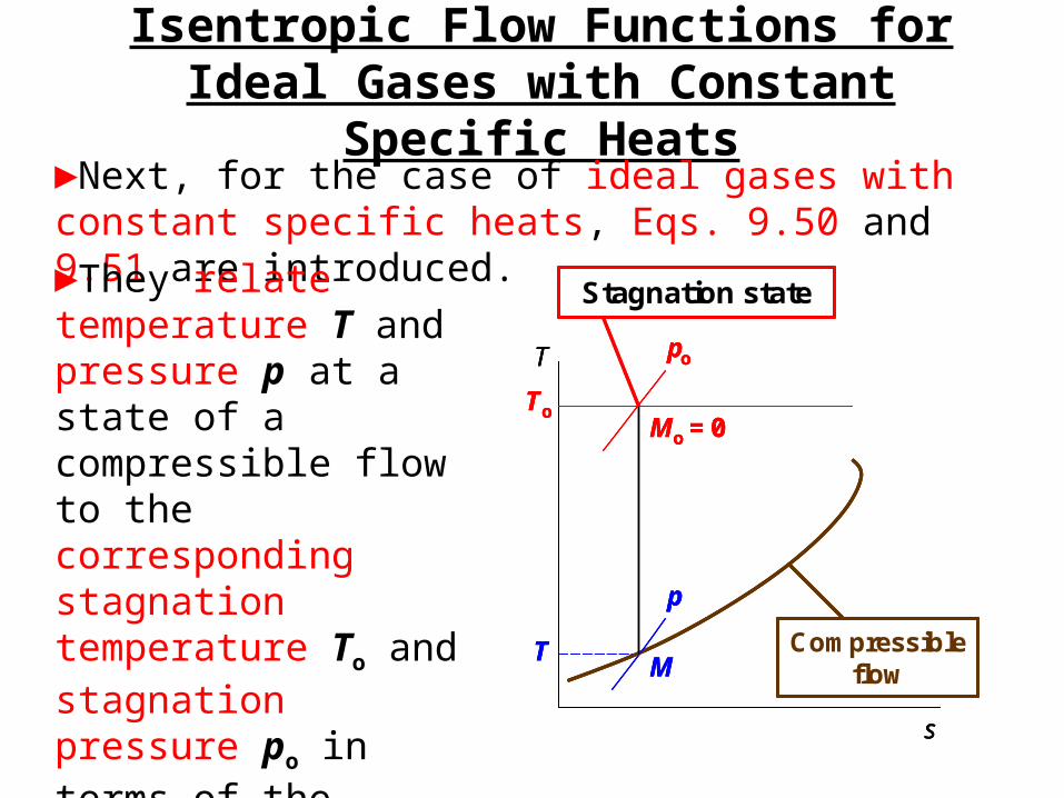
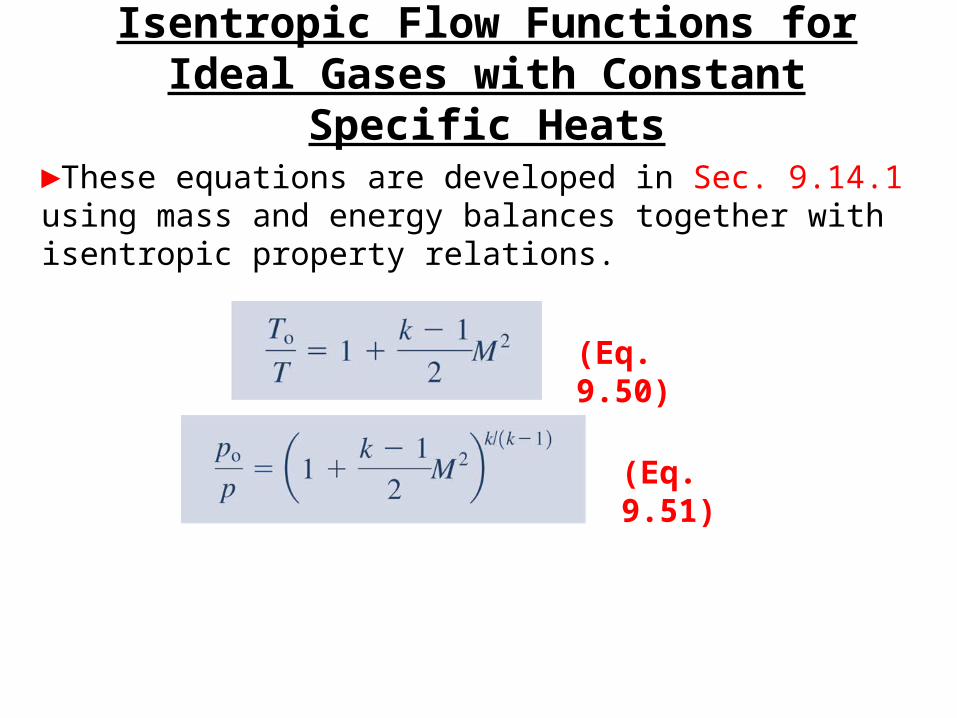
Isentropic Flow Functions for Ideal Gases with Constant Specific Heats
►Next, for the case of ideal gases with constant specific heats, Eqs. 9.50 and 9.51 are introduced.
►They relate temperature T and pressure p at a state of a compressible flow to the corresponding stagnation temperature To and stagnation pressure po in terms of the specific heat ratio k and Mach number M:
Compressibleflow
T
T
s
p
M
To
po
Mo = 0
Stagnation state
Compressibleflow
T
T
s
p
M
To
po
Mo = 0
Compressibleflow
T
T
s
p
M
To
po
Mo = 0
Stagnation state
Isentropic Flow Functions for Ideal Gases with Constant Specific Heats
(Eq. 9.51)
(Eq. 9.50)
►These equations are developed in Sec. 9.14.1 using mass and energy balances together with isentropic property relations.

Isentropic Flow Functions for Ideal Gases with Constant Specific Heats
►Additionally, the cross-sectional area A at a location where the Mach number is M is related to the area A* that – for the same mass flow rate and stagnation state – would be required for sonic flow (M = 1).
►The variation of A/A* with M is shown in the figure for k = 1.4. The figure shows that a unique value of A/A* corresponds to any choice of M.►However, for a given value of A/A* other than unity, there are two possible values for the Mach number, one subsonic and one supersonic.
Variation of A/A* with Mach number in isentropic flow for k = 1.4.
(Eq. 9.52)

Isentropic Flow Functions for Ideal Gases with Constant Specific Heats
►Using Eqs. 9.50-9.52, this tabulation for k = 1.4 – Table 9.2 – can be developed. Use of Table 9.2 for problem solving is illustrated in Example 9.15.►Eqs. 9.50-9.52 are readily programmed for use with hand-held calculators.

Normal Shock Functions for Ideal Gases with Constant Specific Heats
►Consider a normal shock standing in a duct as shown in the figure.
►The ratio of temperature across the shock is
►The ratio of pressure across the shock is
(Eq. 9.54)
(Eq. 9.53)

Normal Shock Functions for Ideal Gases with Constant Specific Heats
►Consider a normal shock standing in a duct as shown in the figure.
►The Mach numbers across the shock are related by
►The ratio of stagnation pressures across the shock is
(Eq. 9.55)
(Eq. 9.56)

Normal Shock Functions for Ideal Gases with Constant Specific Heats
►Using Eqs. 9.53-9.56, this tabulation for k = 1.4 – Table 9.3 – can be developed. Use of Table 9.3 for problem solving is illustrated in Example 9.15.►Eqs. 9.53-9.56 are readily programmed for use with hand-held calculators.