chapter elasticity and its application 5. the elasticity of demand elasticity – measure of the...
Post on 19-Dec-2015
228 views
TRANSCRIPT

Chapter
Elasticity and Its Application
5
The Elasticity of Demand
• Elasticity– Measure of the responsiveness of quantity
demanded or quantity supplied– To one of its determinants
2
The Elasticity of Demand
• Price elasticity of demand– Measure of how much quantity demanded of
a good responds • To a change in the price of that good
– Percentage change in quantity demanded• Divided by the percentage change in price
– Measures how willing consumers are to buy less of the good as its price rises
3
The Elasticity of Demand
• Price elasticity of demand– Elastic demand
• Quantity demanded responds substantially to changes in the price
– Inelastic demand• Quantity demanded responds only slightly to
changes in the price
4
The Elasticity of Demand
• Determinants of price elasticity of demand– Availability of close substitutes
• Goods with close substitutes– More elastic demand
– Necessities vs. luxuries• Necessities – inelastic demand• Luxuries – elastic demand
– Definition of the market• Narrowly defined markets – more elastic demand
– Time horizon– More elastic over longer time horizons
5
The Elasticity of Demand
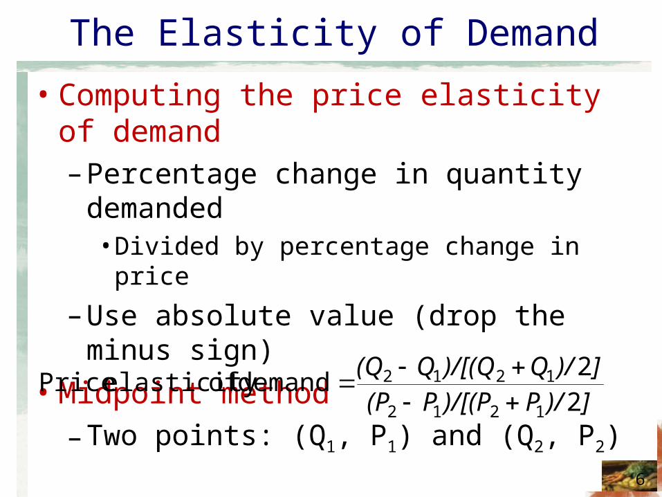
• Computing the price elasticity of demand– Percentage change in quantity demanded
• Divided by percentage change in price
– Use absolute value (drop the minus sign)• Midpoint method
– Two points: (Q1, P1) and (Q2, P2)
6
])/P)/[(PP(P])/Q)/[(QQ(Q
22
1212
1212
demand of elasticity Price
The Elasticity of Demand
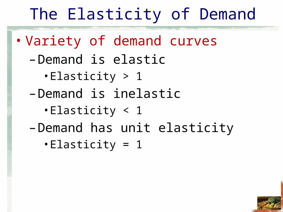
• Variety of demand curves– Demand is elastic
• Elasticity > 1
– Demand is inelastic• Elasticity < 1
– Demand has unit elasticity• Elasticity = 1
7
The Elasticity of Demand
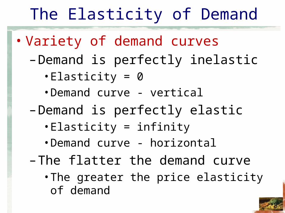
• Variety of demand curves– Demand is perfectly inelastic
• Elasticity = 0• Demand curve - vertical
– Demand is perfectly elastic• Elasticity = infinity• Demand curve - horizontal
– The flatter the demand curve• The greater the price elasticity of demand
8
Figure
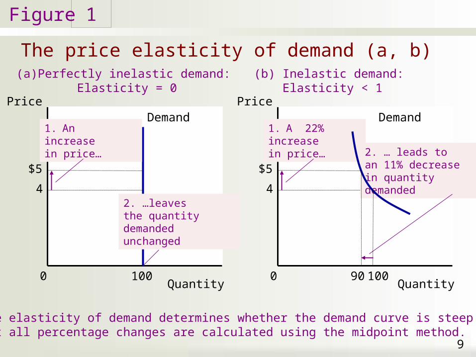
The price elasticity of demand (a, b)
1
9
(a) Perfectly inelastic demand: Elasticity = 0
1. an
Price
Quantity 0
Demand
100
$5
4
1. Anincreasein price…
2. …leavesthe quantitydemanded unchanged
(b) Inelastic demand: Elasticity < 1
1. an
Price
Quantity 0
$5
4
1. A 22%increasein price… 2. … leads to
an 11% decreasein quantitydemanded
Demand
10090
The price elasticity of demand determines whether the demand curve is steep or flat.Note that all percentage changes are calculated using the midpoint method.
Figure
The price elasticity of demand (c)
1
10
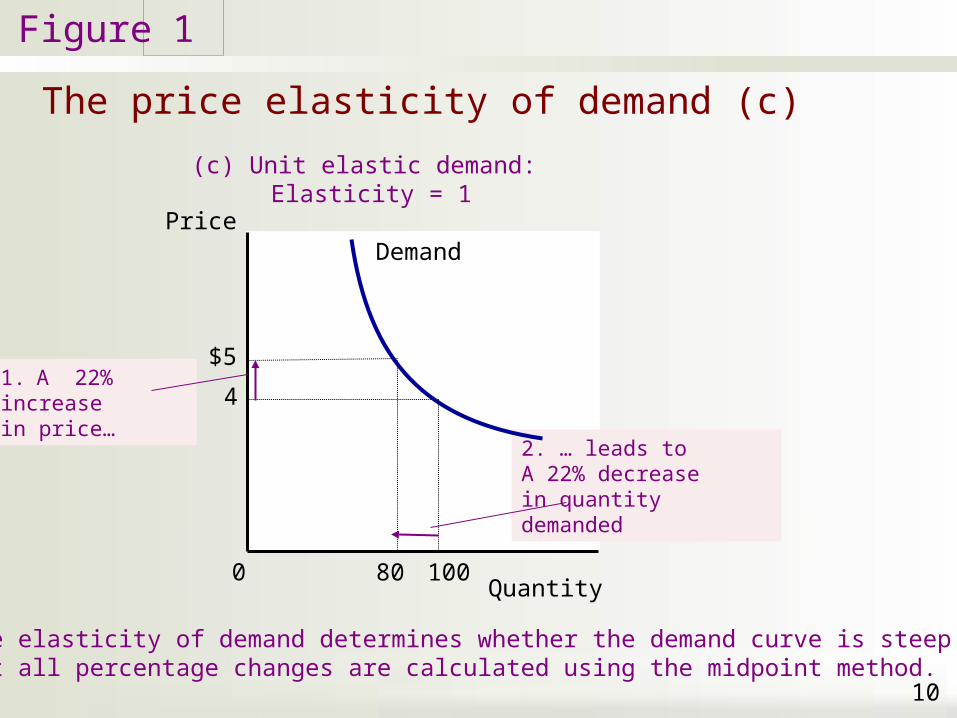
(c) Unit elastic demand: Elasticity = 1
1. an
Price
Quantity 0
$5
41. A 22%increasein price…
2. … leads toA 22% decreasein quantitydemanded
Demand
10080
The price elasticity of demand determines whether the demand curve is steep or flat.Note that all percentage changes are calculated using the midpoint method.
Figure
The price elasticity of demand (d, e)
1
11
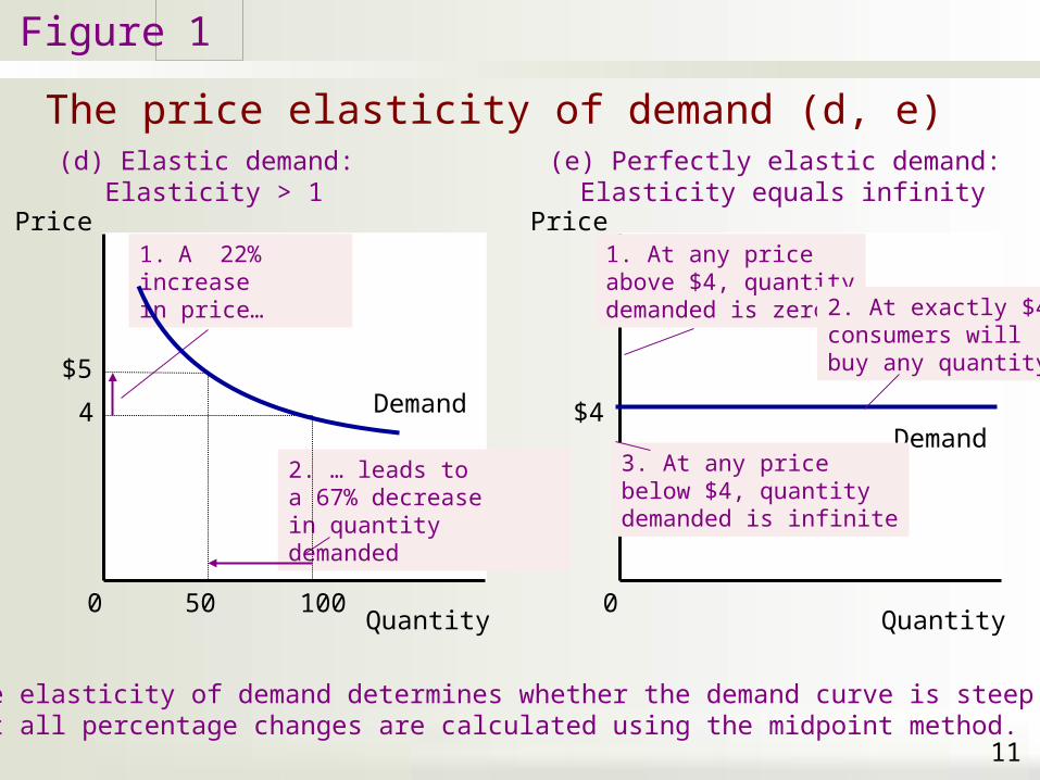
(d) Elastic demand: Elasticity > 1
1. an
Price
Quantity 0
$5
4
1. A 22%increasein price…
2. … leads toa 67% decreasein quantitydemanded
Demand
10050
The price elasticity of demand determines whether the demand curve is steep or flat.Note that all percentage changes are calculated using the midpoint method.
(e) Perfectly elastic demand: Elasticity equals infinity
1. an
Price
Quantity 0
Demand $4
1. At any priceabove $4, quantitydemanded is zero 2. At exactly $4,
consumers willbuy any quantity
3. At any pricebelow $4, quantitydemanded is infinite
The Elasticity of Demand
• Total revenue – Amount paid by buyers– Received by sellers of a good– Computed as: price of the good times the
quantity sold (P ˣ Q)
12
Figure
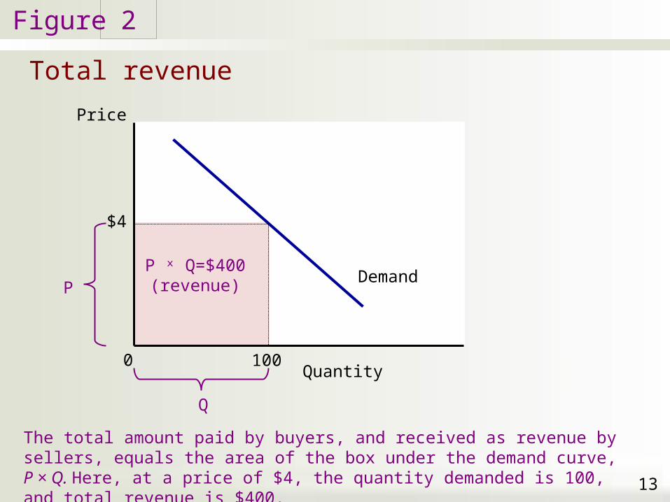
Total revenue
2
13
1. an
P
Q
P ˣ Q=$400(revenue)
Quantity 0
Demand
Price
The total amount paid by buyers, and received as revenue by sellers, equals the area of the box under the demand curve, P × Q. Here, at a price of $4, the quantity demanded is 100, and total revenue is $400.
100
$4
The Elasticity of Demand
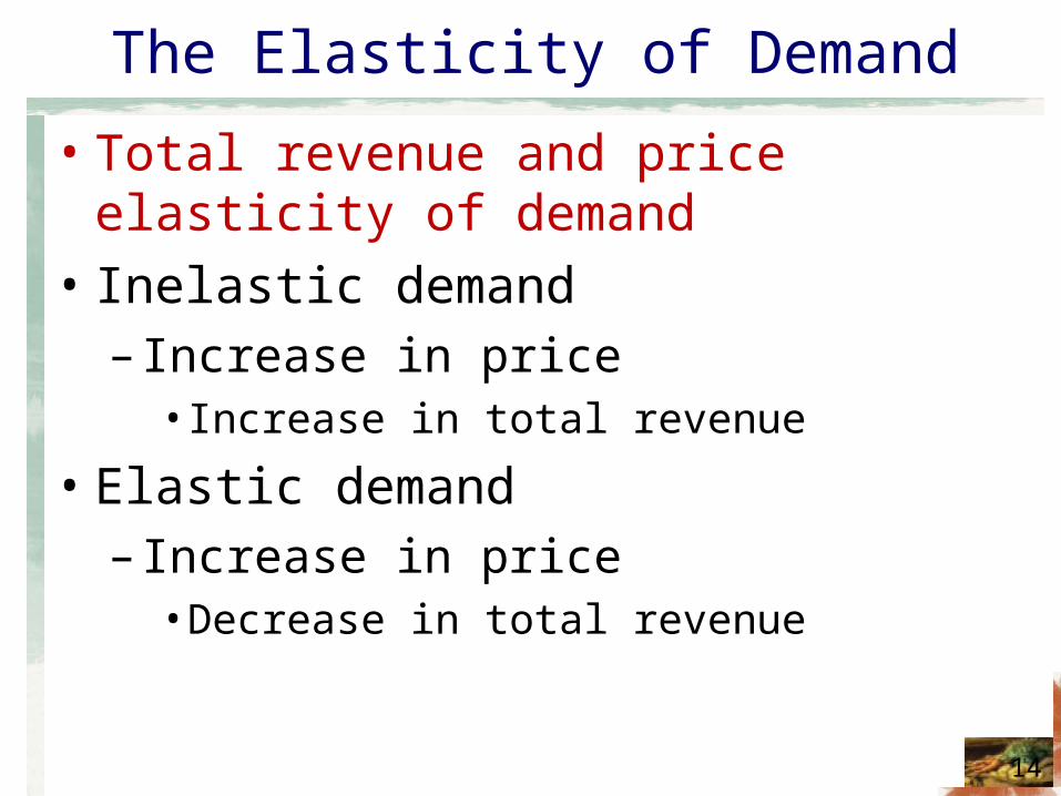
• Total revenue and price elasticity of demand • Inelastic demand
– Increase in price• Increase in total revenue
• Elastic demand– Increase in price
• Decrease in total revenue
14
Figure
How total revenue changes when price changes (a)
3
15
1. an
Revenue=$100
Quantity 0
Demand
Price
100
$1
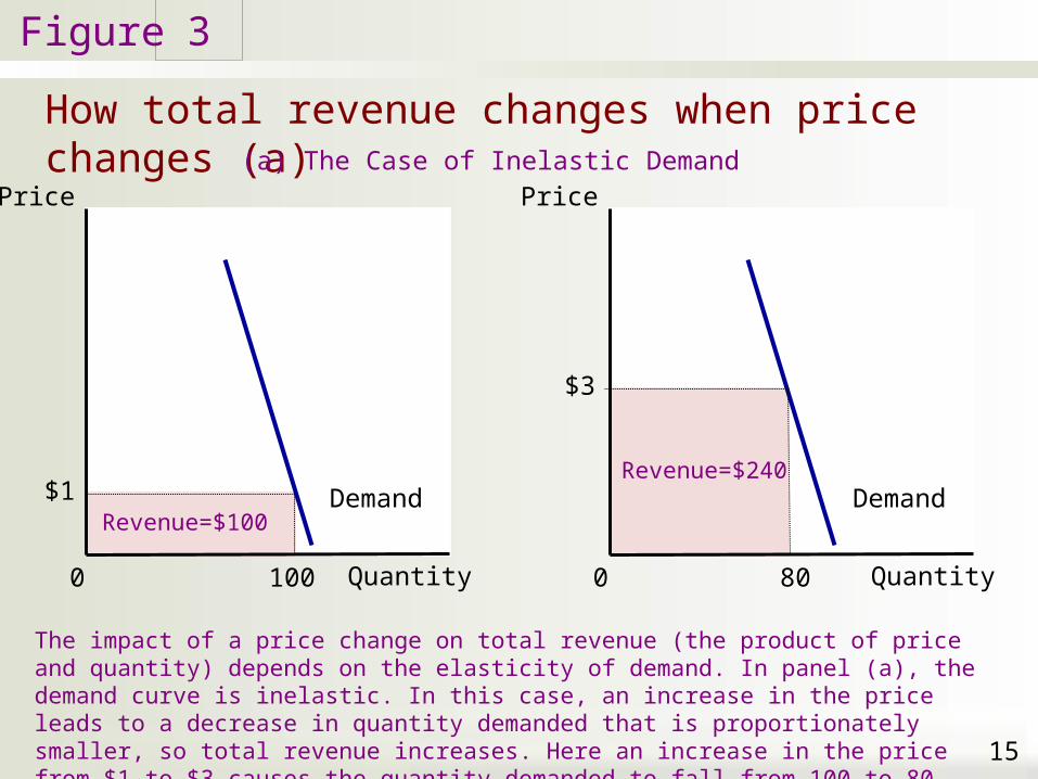
(a) The Case of Inelastic Demand
1. an
Revenue=$240
Quantity 0
Demand
Price
80
$3
The impact of a price change on total revenue (the product of price and quantity) depends on the elasticity of demand. In panel (a), the demand curve is inelastic. In this case, an increase in the price leads to a decrease in quantity demanded that is proportionately smaller, so total revenue increases. Here an increase in the price from $1 to $3 causes the quantity demanded to fall from 100 to 80. Total revenue rises from $100 to $240
Figure
How total revenue changes when price changes (b)
3
16
1. anRevenue
=$200
Quantity 0
Demand
Price
50
$4
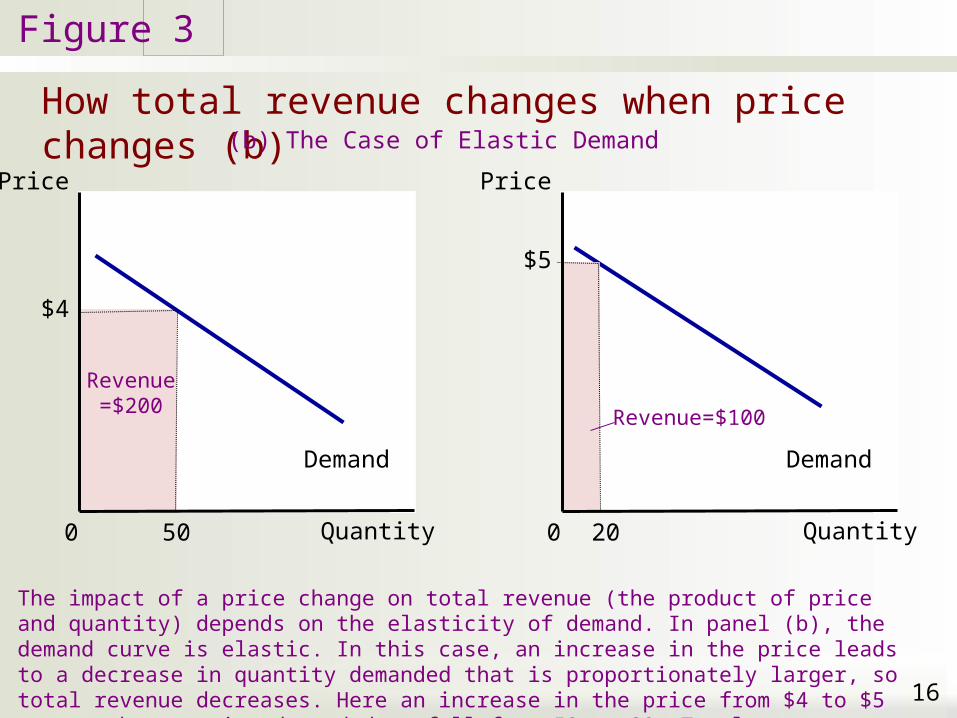
(b) The Case of Elastic Demand
1. an
Demand
The impact of a price change on total revenue (the product of price and quantity) depends on the elasticity of demand. In panel (b), the demand curve is elastic. In this case, an increase in the price leads to a decrease in quantity demanded that is proportionately larger, so total revenue decreases. Here an increase in the price from $4 to $5 causes the quantity demanded to fall from 50 to 20. Total revenue falls from $200 to $100..
Revenue=$100
Quantity 0
Price
20
$5
The Elasticity of Demand
• When demand is inelastic– Price and total revenue move in the same
direction• When demand is elastic
– Price and total revenue move in opposite directions
• If demand is unit elastic– Total revenue remains constant when the
price changes
17

The Elasticity of Demand
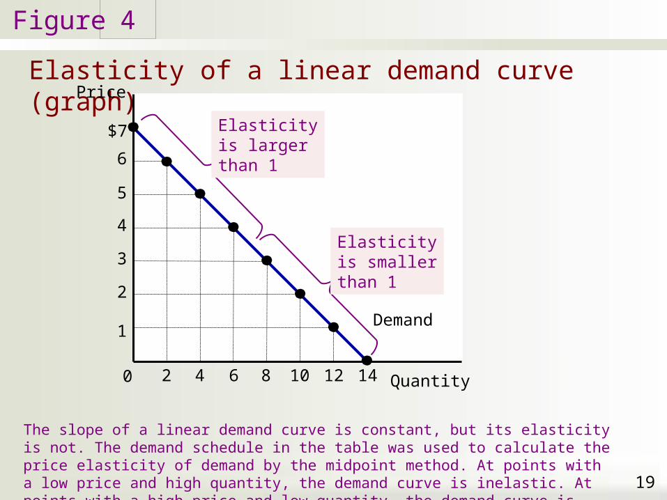
• Elasticity and total revenue along a linear demand curve
• Linear demand curve– Constant slope– Different elasticities
• Points with low price & high quantity– Inelastic
• Points with high price & low quantity– Elastic
18
Figure
Elasticity of a linear demand curve (graph)
4
19
1. an
Quantity 0
Price
Demand
$7
14
6
5
4
3
2
1
2 4 6 8 10 12
Elasticityis largerthan 1
Elasticityis smallerthan 1
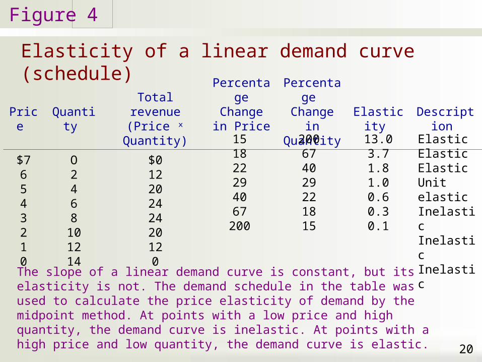
The slope of a linear demand curve is constant, but its elasticity is not. The demand schedule in the table was used to calculate the price elasticity of demand by the midpoint method. At points with a low price and high quantity, the demand curve is inelastic. At points with a high price and low quantity, the demand curve is elastic.
Figure
Elasticity of a linear demand curve (schedule)
4
20
The slope of a linear demand curve is constant, but its elasticity is not. The demand schedule in the table was used to calculate the price elasticity of demand by the midpoint method. At points with a low price and high quantity, the demand curve is inelastic. At points with a high price and low quantity, the demand curve is elastic.
Price Quantity Total revenue
(Price ˣ Quantity)
PercentageChangein Price
Percentage Change inQuantity Elasticity Description
$76543210
O2468
101214
$01220242420120
151822294067
200
200674029221815
13.03.71.81.00.60.30.1
ElasticElasticElasticUnit elasticInelasticInelasticInelastic
The Elasticity of Demand
• Income elasticity of demand– Measure of how much the quantity
demanded of a good responds• To a change in consumers’ income
– Percentage change in quantity demanded • Divided by the percentage change in income
– Normal goods: positive income elasticity• Necessities: smaller income elasticities• Luxuries: large income elasticities
– Inferior goods: negative income elasticities21
The Elasticity of Demand
• Cross-price elasticity of demand– Measure of how much the quantity
demanded of one good responds• To a change in the price of another good
– Percentage change in quantity demanded of the first good• Divided by the percentage change in price of the
second good
– Substitutes: Positive cross-price elasticity– Complements: Negative cross-price elasticity
22
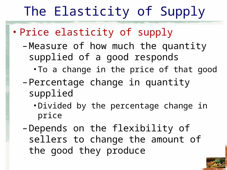
The Elasticity of Supply
• Price elasticity of supply– Measure of how much the quantity supplied
of a good responds• To a change in the price of that good
– Percentage change in quantity supplied• Divided by the percentage change in price
– Depends on the flexibility of sellers to change the amount of the good they produce
23
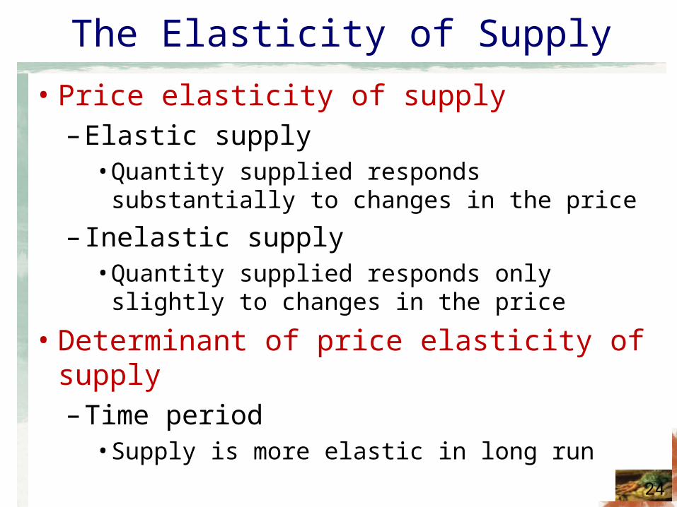
The Elasticity of Supply
• Price elasticity of supply– Elastic supply
• Quantity supplied responds substantially to changes in the price
– Inelastic supply• Quantity supplied responds only slightly to
changes in the price
• Determinant of price elasticity of supply– Time period
• Supply is more elastic in long run24
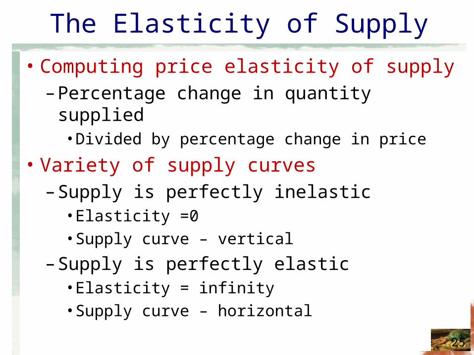
The Elasticity of Supply
• Computing price elasticity of supply– Percentage change in quantity supplied
• Divided by percentage change in price
• Variety of supply curves– Supply is perfectly inelastic
• Elasticity =0• Supply curve – vertical
– Supply is perfectly elastic• Elasticity = infinity• Supply curve – horizontal
25
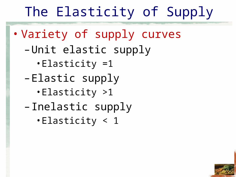
The Elasticity of Supply
• Variety of supply curves– Unit elastic supply
• Elasticity =1
– Elastic supply• Elasticity >1
– Inelastic supply• Elasticity < 1
26
Figure
The price elasticity of supply (a, b)
5
27
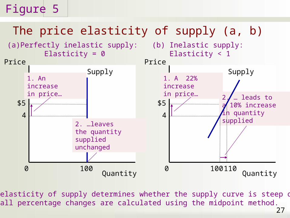
(a) Perfectly inelastic supply: Elasticity = 0
1. an
Price
Quantity 0
Supply
100
$5
4
1. Anincreasein price…
2. …leavesthe quantitysupplied unchanged
(b) Inelastic supply: Elasticity < 1
1. an
Price
Quantity 0
$5
4
1. A 22%increasein price… 2. … leads to
a 10% increasein quantitysupplied
100 110
The price elasticity of supply determines whether the supply curve is steep or flat.Note that all percentage changes are calculated using the midpoint method.
Supply
Figure
The price elasticity of supply (c)
5
28
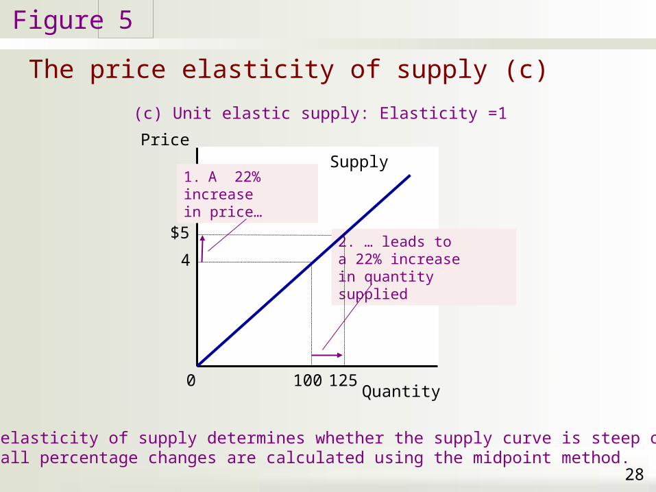
(c) Unit elastic supply: Elasticity =1
1. an
Price
Quantity 0
$5
4
1. A 22%increasein price…
2. … leads toa 22% increasein quantitysupplied
100 125
The price elasticity of supply determines whether the supply curve is steep or flat.Note that all percentage changes are calculated using the midpoint method.
Supply
Figure
The price elasticity of supply (d, e)
5
29
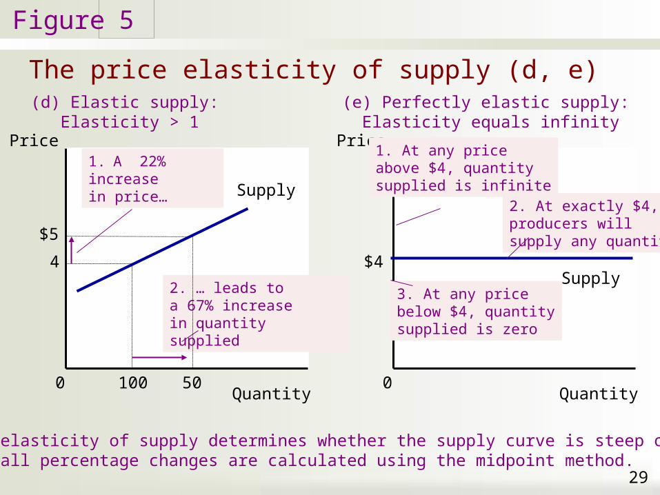
The price elasticity of supply determines whether the supply curve is steep or flat.Note that all percentage changes are calculated using the midpoint method.
(d) Elastic supply: Elasticity > 1
1. an
Price
Quantity 0
$5
4
1. A 22%increasein price…
2. … leads toa 67% increasein quantitysupplied
100 50
(e) Perfectly elastic supply: Elasticity equals infinity
1. an
Price
Quantity 0
Supply $4
1. At any priceabove $4, quantitysupplied is infinite
2. At exactly $4,producers willsupply any quantity
3. At any pricebelow $4, quantitysupplied is zero
Supply
Figure
How the price elasticity of supply can vary
6
30
1. an
Price
Quantity 0
$15
12
Supply
100 525
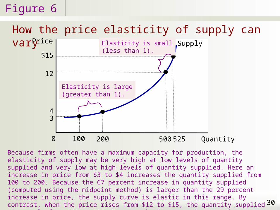
Because firms often have a maximum capacity for production, the elasticity of supply may be very high at low levels of quantity supplied and very low at high levels of quantity supplied. Here an increase in price from $3 to $4 increases the quantity supplied from 100 to 200. Because the 67 percent increase in quantity supplied (computed using the midpoint method) is larger than the 29 percent increase in price, the supply curve is elastic in this range. By contrast, when the price rises from $12 to $15, the quantity supplied rises only from 500 to 525. Because the 5 percent increase in quantity supplied is smaller than the 22 percent increase in price, the supply curve is inelastic in this range.
500200
43
Elasticity is small(less than 1).
Elasticity is large(greater than 1).

Applications of Supply, Demand, & Elasticity
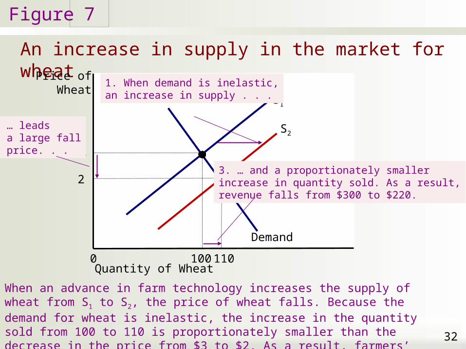
• Can good news for farming be bad news for farmers?– New hybrid of wheat – increase production per
acre 20%• Supply curve changes• Supply curve shifts to the right• Higher quantity; lower price• Demand – inelastic
– Total revenue falls
– Paradox of public policy• Induce farmers not to plant crops
31
Figure
An increase in supply in the market for wheat
7
32
S1
S2
When an advance in farm technology increases the supply of wheat from S1 to S2, the price of wheat falls. Because the demand for wheat is inelastic, the increase in the quantity sold from 100 to 110 is proportionately smaller than the decrease in the price from $3 to $2. As a result, farmers’ total revenue falls from $300 ($3 × 100) to $220 ($2 × 110).
Price ofWheat
Quantity of Wheat0 110
$3
2
100
Demand
1. When demand is inelastic,an increase in supply . . .
2. … leadsto a large fallin price. . .
3. … and a proportionately smallerincrease in quantity sold. As a result,revenue falls from $300 to $220.
Applications of Supply, Demand, & Elasticity
• Why did OPEC fail to keep the price of oil high? – 1970s: OPEC reduced supply of oil
• Increase in prices 1973-1974 and 1971-1981• Short-run: supply is inelastic
– Decrease in supply: large increase in price
– 1982-1990 – price of oil decreased• Long-run: supply is elastic
– Decrease in supply: small increase in price
33
Figure
1. an
Price
1. an
Price
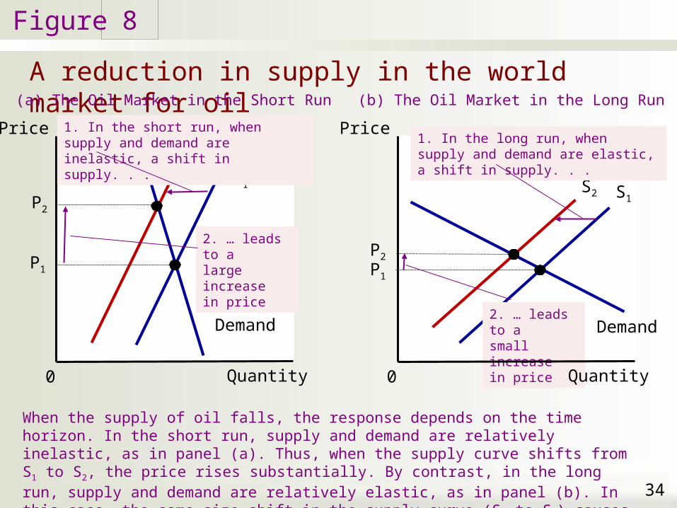
A reduction in supply in the world market for oil
8
34
Demand
P2
(a) The Oil Market in the Short Run
Demand
When the supply of oil falls, the response depends on the time horizon. In the short run, supply and demand are relatively inelastic, as in panel (a). Thus, when the supply curve shifts from S1 to S2, the price rises substantially. By contrast, in the long run, supply and demand are relatively elastic, as in panel (b). In this case, the same size shift in the supply curve (S1 to S2) causes a smaller increase in the price.
(b) The Oil Market in the Long Run
S1
S2
P1
1. In the short run, when supply and demand are inelastic, a shift in supply. . .
2. … leads to alarge increasein price
P2
S1S2
P1
1. In the long run, when supply and demand are elastic, a shift in supply. . .
2. … leads to asmall increasein price
Quantity 0 Quantity 0

Applications of Supply, Demand, & Elasticity
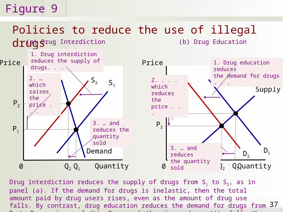
• Does drug interdiction increase or decrease drug-related crime?– Government increases the number of federal
agents devoted to the war on drugs• Illegal drugs - Supply curve shifts left
– Higher price; lower quantity
– Amount of drug-related crimes• Inelastic demand for drugs• Higher drugs price – higher total revenue• Increase drug-related crime
35

Applications of Supply, Demand, & Elasticity
• Does drug interdiction increase or decrease drug-related crime?– Policy of drug education
• Reduce demand for illegal drugs• Left shift of demand curve• Lower quantity; lower price• Reduce drug-related crime
36
Figure
Policies to reduce the use of illegal drugs
9
37
1. an
Price
1. an
Price
Demand
P2
(a) Drug Interdiction
D1
Drug interdiction reduces the supply of drugs from S1 to S2, as in panel (a). If the demand for drugs is inelastic, then the total amount paid by drug users rises, even as the amount of drug use falls. By contrast, drug education reduces the demand for drugs from D1 to D2, as in panel (b). Because both price and quantity fall, the amount paid by drug users falls
(b) Drug Education
S1S2
P1
1. Drug interdiction reduces the supply of drugs. . .
2. … whichraises theprice . . .
P2
Supply
P1
1. Drug education reducesthe demand for drugs . . .
2. . . . whichreduces theprice . . .
Quantity 0 Quantity 0Q1Q2
3. … and reduces the quantity sold
D2
Q1Q2
3. … and reducesthe quantity sold