chapter four modeling and design
TRANSCRIPT

154
~Chapter Four
Modeling and Design~

155
This chapter describes how, utilizing the technology described in previous chapters, a fuel cell
scooter may be designed. It leads from an analysis of performance requirements to a vehicle model
to a systems design of the fuel cell stack and auxiliary systems. The model uses basic assumptions
to obtain an overall measure of performance; parasitic power is a linear function of gross power,
and conservative assumptions are made where data is poorly known.
Two additional options for improved performance and reduced cost, respectively, are considered:
operation of the fuel cell at 3 atm pressure, and hybridization with peaking power batteries.
A different kind of scooter – a zinc-air battery-powered alternative – is considered as well because
electric scooter manufacturers and researchers in Taiwan are extremely interested in this
technology
156
4.1 Performance requirements
Despite the attraction they offer in the form of zero emissions, battery-powered electric vehicles
have failed to capture significant market shares because they are inconvenient to recharge, and
because they simply do not match the performance of existing alternatives. The important
performance criteria are vehicle range before refueling, power, cost, and to a lesser extent vehicle
weight.
The performance characteristics of a few sample vehicles with similar power needs are summarized
here as a baseline for the fuel cell scooter; they range from ordinary gasoline scooters to prototype
electric scooters to a much heavier demonstration fuel cell - powered golf cart which is included
because it is virtually the only PEM fuel cell vehicle designed at the 4-6 kW power output level.
Note that the motor power quoted here is the mechanical power generated; battery or fuel cell
output will typically be larger by a factor of 30% due to drivetrain losses.

157
Table 4.1. Performance of various vehicles of about 5 kW power
Vehicle
Fuel cellelectricgolf cart
Battery-poweredelectric scooter(NiCd battery)
Medium-sized two-stroke
scooter
Battery-poweredelectric scooter
(lead-acid)
name Schatz “Personal Utility Vehicle”
Honda CUV ES
HondaDio
Taiwan ITRIZES-2000
maximummotor power
1.5 kW (4.0 kW fuel cell)
3.2 kW 5 kW 3.4 kW
range at 30 km/h cruise
24 km 35 km 240 km(5 L tank)
60 km
fuel efficiencyat 30 km/h cruise
96 mpge 1000 mpge( 46.2 km/kWh)
116 mpg 1300 mpge(60 km/kWh)
acceleration – 0-200 m in17.3 seconds
~0-50 m in6 seconds
0-30 m in 4.5 seconds
maximum speed 20 km/h 60 km/h ~70 km/h 50 km/h
charging time 2 minute cylinderrefilling
8 hoursfull recharge
5 minutegasoline refill
8 hoursfull recharge
hill climbing – – – 15 km/hat 10( slope
curb weight 380 kg 130 kg 68 kg 105 kg
Taiwan data is from reports published by the Industrial TechnologyResearch Institute1. Honda vehicle data are from a Society ofAutomotive Engineers of Japan paper and a paper published by theITRI.2,3 The Schatz Energy Research Center’s Personal Utility Vehiclewas documented in a 1998 Fuel Cell Seminar abstract, and the weightwas from a data sheet for that E-Z Go 4Caddy electric golf cart.4,5
Performance measurements marked with tildes were for 50 cc scooterssimilar to the Dio as data were not directly available.
“curb weight” is the mass of the vehicle without passengers or cargo.
The unusual acceleration measurement (time required to cover a givendistance) is a standard for scooters in Asia.
Note that the Dio’s 5 kW engine is at the high end of 50 cc vehicles. Many 50 cc scooters have
powers of 2-4 kW, while 125 cc scooters produce 6-9 kW of power.
“mpge” (miles per gallon equivalent) fuel economies for the non-combustion vehicles were

158
calculated by taking the total energy stored – whether as chemical energy in a battery or in terms of
hydrogen lower heating value – and calculating how many gallons of gasoline would have to be
burned to produce the same amount of heating value energy. This “on-vehicle” fuel economy is
slightly misleading in that hydrogen and batteries tend to be higher grade carriers of energy; that is,
it would take a large amount of energy from burned petroleum to store the same energy in
hydrogen or battery form. Later wells-to-wheels fuel efficiency calculations will take into account
the conversion losses.
Nakazawa et al claim that the Honda CUV-ES’s 35 km range under an urban driving cycle is
“sufficient for practical use.”2 Researchers from Taiwan’s ITRI (Industrial Technology Research
Institute) also claim that daily driving ranges are less than 25 km 68% of the time, and 70% of the
daily driving time is less than one and a half hours.6 But, as a point of comparison, a gasoline
scooter of similar power (i.e. one with 50 cc displacement) achieves quadruple the range of even
the best electric scooters when being driven at a steady speed of 30 km/h. A 35 km range may be
enough for use, but electric scooters will never replace a third of two-stroke scooters if their
competitors have four times the range with quicker refueling. A more reasonable set of
requirements would be to preserve the same minimum acceleration characteristics, but to require
that the range be at least 200 km. A range of over 240 km like the Dio is optimal, but probably not
necessary and expensive in terms of dollars and volume.
The power of 4-6 kW is relatively high for a lightweight and small vehicle like the scooter, but this
is due to the way in which scooters are driven under typical urban conditions. Bursts of rapid
acceleration are used to dodge in between larger vehicles in congested traffic, and quick starts are
often required when red lights turn green. Frequent decelerations and stops are needed in the city,
and scooters are not often taken out on the highway for prolonged high-speed driving. Basically,
159
average speeds and average power are low, but peak power is high.
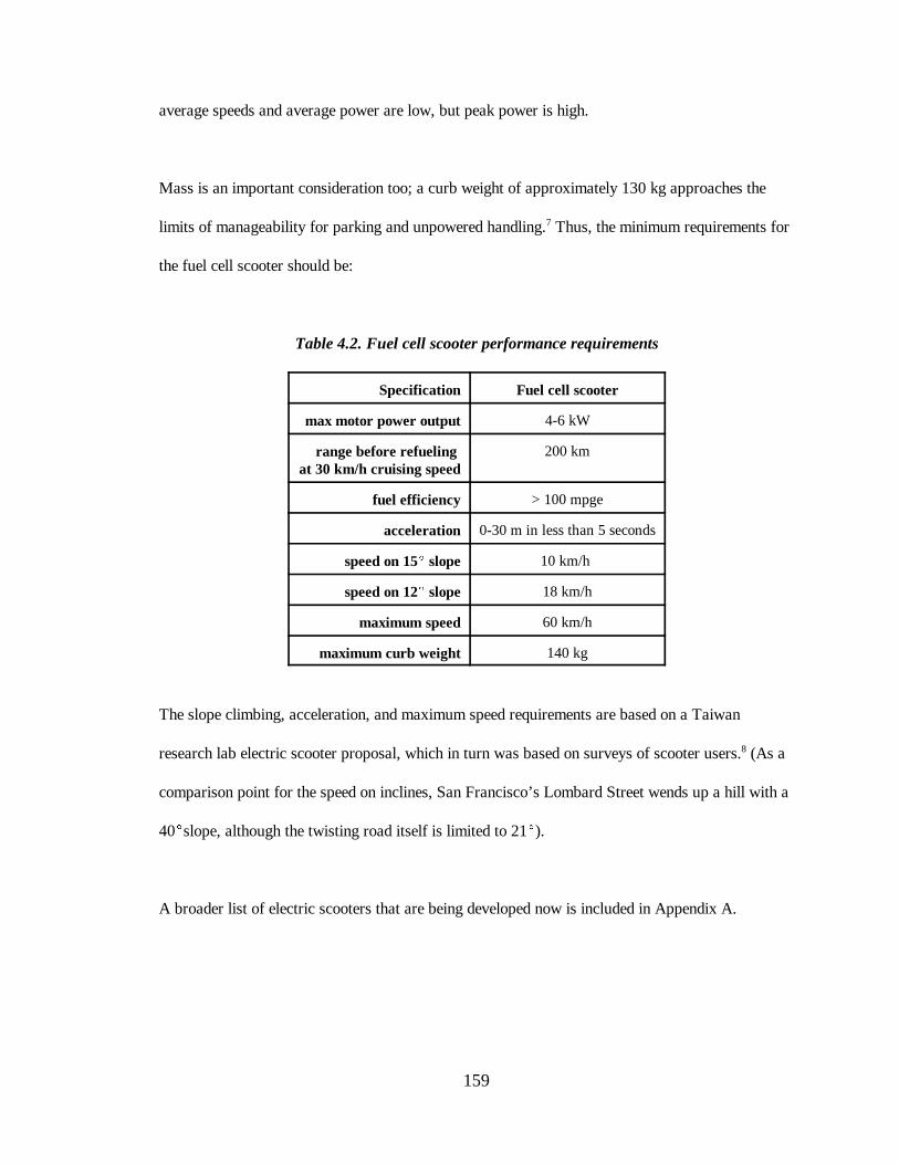
Mass is an important consideration too; a curb weight of approximately 130 kg approaches the
limits of manageability for parking and unpowered handling.7 Thus, the minimum requirements for
the fuel cell scooter should be:
Table 4.2. Fuel cell scooter performance requirements
Specification Fuel cell scooter
max motor power output 4-6 kW
range before refueling at 30 km/h cruising speed
200 km
fuel efficiency > 100 mpge
acceleration 0-30 m in less than 5 seconds
speed on 15(( slope 10 km/h
speed on 12(( slope 18 km/h
maximum speed 60 km/h
maximum curb weight 140 kg
The slope climbing, acceleration, and maximum speed requirements are based on a Taiwan
research lab electric scooter proposal, which in turn was based on surveys of scooter users.8 (As a
comparison point for the speed on inclines, San Francisco’s Lombard Street wends up a hill with a
40(slope, although the twisting road itself is limited to 21().
A broader list of electric scooters that are being developed now is included in Appendix A.

160
4.2 Vehicle modeling
Essentially, the purpose of vehicle modeling is to convert input parameters (performance
measurements like desired range, driving cycle that must be sustained, and types of power and
storage components) into the output parameters of curb weight, size of engine required, heating
system design, cost, and convenience. The process is iterative; for example, the size of the cooling
system is a function of the average vehicle power, but larger cooling system itself requires more
power to drive the fans and pumps, increasing the power load, which necessitates more cooling.
4.2.1 Physical model
To properly simulate the performance of a fuel cell scooter, a computer model was created based
on the physical properties of the scooter. This model calculates the instantaneous power required
from a scooter’s engine as it travels through various driving patterns, and derives various
numerical performance characteristics: fuel consumed per kilometer of travel, maximum power
during the driving cycle, average power during the driving cycle, amount of energy recovered in
regenerative braking, and overall hydrogen-to-mechanical-work conversion efficiency.
For the MATLAB program listing, please see Appendix F.
This power is calculated as the dot product of the current velocity of the vehicle and the various
forces acting upon it, divided by the motor and controller efficiency, plus the auxiliary power
demanded by various lighting and control systems, plus “parasitic” power required by the fuel cell
blowers and coolant pumps. The road is assumed to be level. There are several different physical

161
forces to consider: air resistance (drag); the rolling resistance of the wheels; the force of gravity,
which is not necessarily perpendicular to the velocity if the vehicle is traveling uphill or downhill;
and the normal force of the ground acting upon the vehicle. These forces must sum to zero if the
vehicle is to be held at a constant velocity, or to a net forward acceleration times mass if the vehicle
is to accelerate.
Figure 4.1 Free-body diagram of scooter
In the computer model used to simulate vehicle performance, the various power demands are
summed to a total mechanical power Pwheels demanded “at the wheels” by the motion of the vehicle.
Pwheels = ( mav) +( mgvsin� ) + ( mgvCRR cos� ) + ( ½ 'ai rCD AF v3 )
The variables are listed below.
162
m = total mass of vehicle, passengers and cargo
� = angle of slope
a = acceleration of vehicle
v = velocity of vehicle
CRR = coefficient of tire rolling resistance.
'air = density of air, approximately 1.23 kg•m-3
CD = drag coefficient
AF = frontal area
The terms are described one at a time:
Acceleration term. If the acceleration is negative - that is, the vehicle is decelerating - the first term
can be negative. If the overall expression for Pwheels is still positive even though the first term is
negative, it means that energy must still be supplied by the power source to the wheels to maintain
the desired deceleration rate, because the drag and rolling resistances are so large. If Pwheels is
negative, then the motor can be driven as a generator to regenerate some of the energy expended. A
battery capable of reabsorbing this energy is needed, and less than 70% of the kinetic energy is
recoverable. This figure is reduced if rapid deceleration is required, because the battery can only
charge up at a certain maximum rate.
Slope term. The second term is the force of gravity resolved opposite to the direction of motion.
Rolling resistance term. The coefficient of rolling resistance is a function of tire pressure and
deformation, and is the ratio of rolling resistance force to the load on the tires; it is fairly constant
for a given tire.9 A perfectly rigid wheel on a rigid, flat surface would have no rolling resistance,

163
but minor deformations in the wheel and properties of the road cause deviation from ideal geometry
and thus irreversible losses.
Aerodynamic drag term. The drag coefficient CD is a dimensionless constant that attempts to
capture, in one term, an object's resistance to flow. CD can vary from as high as 1.2 for a bicycle
with erect rider to 0.47 for a sphere to 0.20 for a very aerodynamically-styled modern
automobile.10 Although the equation used to determine the drag power is a simplification, it avoids
complex air flow simulation while preserving the general behaviour of the drag force with respect
to velocity. The frontal area used here was measured for the scooter by projecting a bright light
parallel to the front of the scooter and then measuring the area of the shadow on a wall behind.11
Typical values are listed in Table 4.3.
The inefficiencies in the system are applied afterwards to determine how much power must be put
out by the power source:
Poutput = (Pwheels)/�drivetrain + Pauxiliary + Pparasitics
Pauxiliary = power needed by auxiliary systems - headlights, signal lights, dashboard, etc.
�drivetrain = efficiency of the electric motor and controller subsystem - 77%
Pparasitics = parasitic power needed by fuel cell system - blowers, fans, etc.
The parasitic and auxiliary powers are electric power requirements so they do not go through the
77% efficiency loss. A more sophisticated model would not use a single value of �drivetrain but rather
employ an efficiency map to determine electric motor efficiency as a function of wheel speed and
torque.

164
Factors not accounted for in this model include: turning, where the velocity is not parallel to the
acceleration / deceleration direction; wind blowing at an angle to the direction of motion;
resistances in other parts of the scooter. Friction in the transmission and similar losses are assumed
to be captured by the drivetrain efficiency of 77% above, discussed in section 2.1.4.
4.2.2 Modeling parameter selection
Vehicle modeling parameters for a typical scooter are listed below with data for other vehicles for
comparison. Although most two-stroke scooters weigh about 80 kg, the presence of lead-acid
batteries and/or fuel cell plus hydrogen storage brings the mass of an electric scooter up to
approximately 130 kg as in the case of the Honda CUV-ES with NiCd batteries.
Table 4.3. Typical modeling parameters
Vehicle CRR CD AF (m2)curb
weight (kg)auxiliary power (W)
Electric Scooter 0.014 0.9 0.6 130 60
Roadster Bicycle 0.008 1.2 0.5 10 0
Motorcycle unknown 0.6 0.8 300 unknown
Ford AIV Sable 0.0092 0.33 2.13 1291 500
PNGV Automobile 0.007 0.20 2.0 920 400
The PNGV Automobile properties are targets set out by thePartnership for a New Generation of Vehicles,12 except for the rollingresistance and auxiliary power which were obtained from separatestudies.13,14 The Ford AIV Sable is a light weight “aluminum intensivevehicle”, a modern mid-sized sedan.15 Motorcycle data was obtainedfor some of the parameters.16 Finally, the bicycle data is for a“roadster”upright model.10
The scooter coefficient of tire rolling resistance was estimated to be 0.014, based on measurements
done at the Desert Research Institute17, while the drag coefficient and frontal area were obtained

165
from researchers at the ITRI Mechanical Industry Research Laboratory.18 A slight mass
dependence (less than 6%) in the drag coefficient reported by the MIRL researchers was ignored,
and the largest measurement taken; the velocity dependence of the rolling resistance coefficient was
likewise neglected. Note also that in scooters and bicycles the product of drag coefficient and
frontal area can vary dramatically, depending on how the driver sits on the scooter. The values
chosen were assumed to be for the rider in a typical position.
The curb weight was set at 130 kg, which was 30 kg more than the ZES-2000 but equal to that of
the CUV-ES electric scooter. This choice was made to ensure that performance requirements
would be met even if the lower ZES-2000 weight could not be reached, whether due to the extra
structural weight needed to support the heavier power system, or due to the weight of the
components themselves. The driver weight is defined as 75 kg.
Auxiliary power: in a typical scooter, the head lights, tail lights, and dashboard total about 50 W;
assuming that these lights are always on, and that the 26.4 W turn lights are on 30% of the time,
yields an average load estimate of 60 W.19
4.2.3 Relative importance of various factors
Now that the parameters are defined, power requirements are calculated for (i) a scooter traveling
at constant velocity at various slopes, and (ii) a scooter traveling with constant velocity at various
speeds, and finally (iii) power required for various accelerations starting from 30 km/h. The total
power shown below is the electric output from the power source including auxiliary power, but not
subsystem parasitic loads (blowers, pumps, etc.) which are calculated later.

166
615 W at30 km/h
0
500
1000
1500
2000
2500
3000
pow
er (
W)
0 5 10 15 20 25 30 35 40 45 50 55 60
speed (km/h)
auxiliary power rolling resistance aerodynamic drag
0
1000
2000
3000
4000
pow
er (
W)
0 2 4 6 8 10 12 14 16 18 20slope (degrees)
aerodynamic drag rolling resistance
auxiliary power slope effect
Figure 4.2. Cruising power required at various speeds.
Figure 4.3. Power required to climb various slopes at 15 km/h
167
0
1000
2000
3000
4000
5000
6000
pow
er (
W)
0.0 1.0 2.0 3.0 4.0 5.0 6.0 7.0 8.0acceleration (km/h/s)
rolling resistance aerodynamic drag
auxiliary power power to accelerate
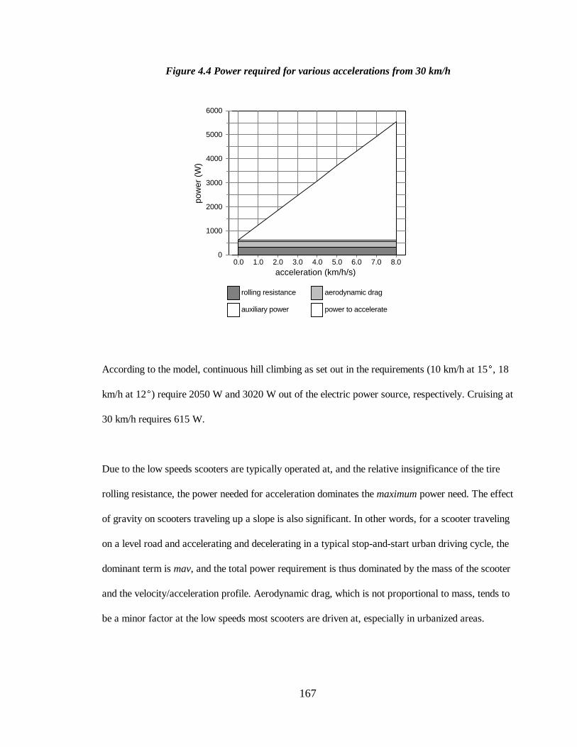
Figure 4.4 Power required for various accelerations from 30 km/h
According to the model, continuous hill climbing as set out in the requirements (10 km/h at 15(, 18
km/h at 12() require 2050 W and 3020 W out of the electric power source, respectively. Cruising at
30 km/h requires 615 W.
Due to the low speeds scooters are typically operated at, and the relative insignificance of the tire
rolling resistance, the power needed for acceleration dominates the maximum power need. The effect
of gravity on scooters traveling up a slope is also significant. In other words, for a scooter traveling
on a level road and accelerating and decelerating in a typical stop-and-start urban driving cycle, the
dominant term is mav, and the total power requirement is thus dominated by the mass of the scooter
and the velocity/acceleration profile. Aerodynamic drag, which is not proportional to mass, tends to
be a minor factor at the low speeds most scooters are driven at, especially in urbanized areas.
168
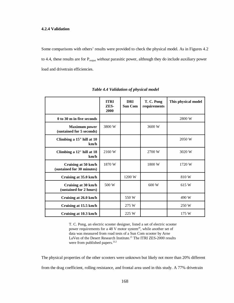
4.2.4 Validation
Some comparisons with others’ results were provided to check the physical model. As in Figures 4.2
to 4.4, these results are for Poutput without parasitic power, although they do include auxiliary power
load and drivetrain efficiencies.
Table 4.4 Validation of physical model
ITRIZES-2000
DRISun Com
T. C. Pongrequirements
This physical model
0 to 30 m in five seconds 2800 W
Maximum power(sustained for 5 seconds)
3800 W 3600 W
Climbing a 15(( hill at 10km/h
2050 W
Climbing a 12(( hill at 18km/h
2160 W 2700 W 3020 W
Cruising at 50 km/h(sustained for 30 minutes)
1870 W 1800 W 1720 W
Cruising at 35.0 km/h 1200 W 810 W
Cruising at 30 km/h(sustained for 2 hours)
500 W 600 W 615 W
Cruising at 26.0 km/h 550 W 490 W
Cruising at 15.5 km/h 275 W 250 W
Cruising at 10.3 km/h 225 W 175 W
T. C. Pong, an electric scooter designer, listed a set of electric scooterpower requirements for a 48 V motor system20, while another set ofdata was measured from road tests of a Sun Com scooter by ArneLaVen of the Desert Research Institute.21 The ITRI ZES-2000 resultswere from published papers.22,2
The physical properties of the other scooters were unknown but likely not more than 20% different
from the drag coefficient, rolling resistance, and frontal area used in this study. A 77% drivetrain

169
0
500
1000
1500
2000
2500
pow
er (
W)
0 5 10 15 20 25 30 35 40 45 50 55 speed (km/h)
model ITRI DRI data T.C. Pong
efficiency was assumed for the ZES-2000, since these data were based on motor output; the other
data points were from battery output measurements, and thus no drivetrain efficiency had to be
assumed. The tabulated results are presented graphically below.
Figure 4.5 Validation of physical model
To verify the model in a different way, the cruising power of 615 W for 30 km/h was used to
calculate average thermal efficiency if the drivetrain efficiency was also 77% for a mechanical
system, and net fuel economy was 100 mpge as reported by various manufacturers. This means an
average 9.5% thermal efficiency, a reasonable estimate for small two-stroke engines (As an
example, a 34 cc engine designed for a blower, hedge trimmer, or chain saw has a peak thermal
efficiency of 13.6%, or 20.6% for a prototype advanced stratified lean-burn design.23)
If a 50% fuel cell conversion efficiency is assumed and parasitic losses are not included yet, then the
equivalent fuel economy is 560 mpge; detailed analysis later will provide a more accurate result.

170
4.3 Driving Cycle
The main purpose of driving cycles, in the past, was to provide a schedule to put cars through to
collect tailpipe emissions and, in the United States, to compute mileages for CAFE (Corporate
Average Fuel Economy). Simulated driving patterns have high-power peaks that produce more
emissions than a constant driving speed, and are more representative of actual driving behaviour.
The typical procedure is to place the vehicle on a wheeled dynamometer and then to execute the
driving cycle. Emissions are collected in a sampling bag and diluted with a predefined amount of air
to obtain vehicle emissions in terms of grams per kilometer.
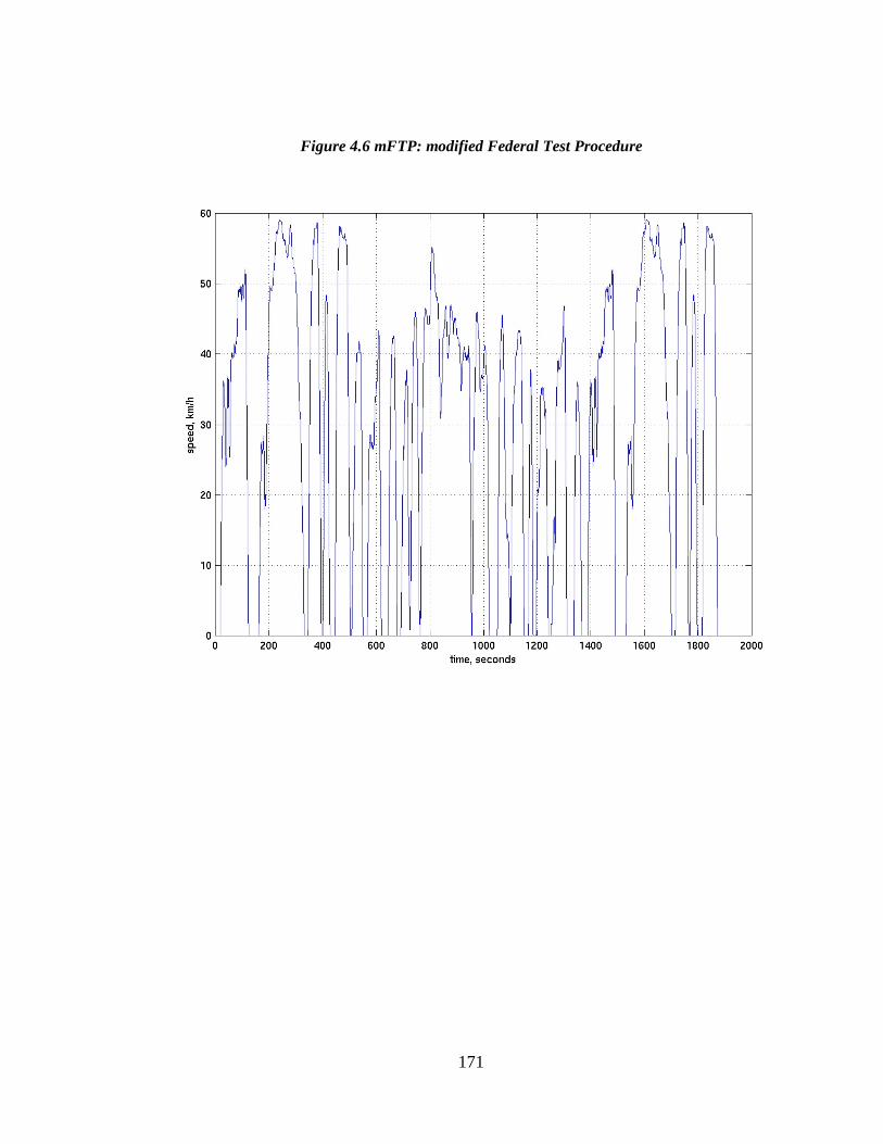
Typical automobile test cycles include the American FUDS (Federal Urban Driving Schedule),
FHDS (Federal Highway Driving Schedule), and FTP (Federal Test Procedure 1975). American
motorcycles are tested using a modified version of FTP (“mFTP”), with one part scaled down for
motorcycle with engines less than 170 cc, so that the maximum speed is reduced from 91 km/h to 59
km/hr. Another method for testing motorcycles is the ECE-40 (Economic Commission for Europe)
test procedure, which employs a much simpler and more abstracted driving cycle. Low acceleration
rates and lack of transients mean that pollution is generally underestimated.
171
Figure 4.6 mFTP: modified Federal Test Procedure

172
Figure 4.7 ECE-40
In recent years, driving cycles have been paired with computer models of road load, as described
above, to predict and model vehicle performance.
4.3.1 TMDC
Driving patterns in Asian cities are significantly different from American highway driving, and even
American city driving. For example, Taipei’s congestion and frequent stops mean that average
driving speed is less than 15 km•h-1, and driving speed exceeds 40 km•h-1 only 10% of the time.24
The driving cycle used here, therefore, should be specifically targeted for the Asian driver. One

173
candidate is the Taipei Motorcycle Driving Cycle (TMDC), developed by researchers at the
Institute of Traffic and Transportation at Taiwan’s National Chiao Tong University. The TMDC is
an actual velocity trace obtained by researchers who followed target vehicles on an instrumented
“chase vehicle”. The driving cycle consists of 950 velocity measurements (one per second) and each
velocity measurement is rounded to the near km•h-1. An acceleration profile was derived by taking
finite differences in temporally-adjacent velocity measurements.
Figure 4.8 Taipei Motorcycle Driving Cycle (TMDC)

174
As a comparison of several characterizing parameters shows, the TMDC is different from FUDS
and the motorcycle-modified FTP:
Table 4.5 Driving Cycle Comparison
TMDCmodified
FTP FUDS
Total time 950 s 1873 s 1372 s
Total distance traveled 5109 m 15537 m 7450 m
Average speed 19.3 km/h 29.9 km/h 19.6 km/h
Maximum speed 46 km/h 59 km/h 57 km/h
Maximum acceleration 13.0 km/h/s 5.4 km/h/s 3.6 km/h/s
Maximum deceleration -15.0 km/h/s -5.4 km/h/s -3.3 km/h/s
Fraction of time spent accelerating 31.5% 42.7% 39.7%
Fraction of time spent decelerating 30.3% 56.3% 34.6%
Fraction of time at steady non-zero speed 18.5% 1.0% 6.6%
Fraction of time at standstill (v = 0) 19.7% 15.2% 19.0%
The TMDC exhibits especially severe accelerations and decelerations - maximums of +13.0 km/h/s
and -15.0 km/h/s, respectively. The maximum acceleration in the modified FTP cycle often used for
testing vehicle emissions is 5.4 km/h/s, but the maximum acceleration observed in Bangkok
motorcycle traffic is quoted as being 12 km/h/s.25 (It is not clear what size of motorcycle the
Bangkok number refers to). While it is true that scooters in Taiwan are driven in a more aggressive
way than cars in American cities, these accelerations and their consequent power requirement of
over 12 kW at the wheels significantly exceed the maximum performance capabilities of scooters
125 cc or less.
One important ramification of the high accelerations and decelerations is that a significant amount

175
of energy can theoretically be recovered by regenerative braking. Also, maximum power is much
larger than average power.
Note also in Figure 4.8 “jitter” in the velocity reading. Errors due to rounding of the speedometer
reading to the nearest km/h when the data was recorded create exaggerated accelerations and
decelerations that did not reflect reality. For example, a speed that varied from 20.4 to 20.6 and
back to 20.4 in two seconds would appear in the data as a one-second acceleration from 20 to 21
and back to 20. This jitter was analyzed below using the scooter model described previously. (The
jitter starts from the base speed and oscillates up and down by 1 km/h)
Table 4.6 Effects of “jitter”
initialspeed
(km/h)
average power to accelerate 1 km/h faster in
1 second, then return to original speed (W)
power if speed was a constant 0.5 km/h faster
(W)
jitter increases power by
this fraction
5 179 117 53%
10 290 177 64%
15 416 252 65%
20 564 348 62%
25 740 472 57%
30 951 632 50%
35 1204 834 44%
40 1507 1085 39%
45 1866 1393 34%
The test shows that these oscillations produce significant variations in power required by the model
that are not representative of actual driving.

176
4.3.2 Modification of TMDC
The TMDC is more representative of Taipei driving conditions than FTP or FUDS, but it has flaws
that should be compensated for. As given, to achieve the performance of the TMDC simulation, a
total power output of more than 12 kW is needed, significantly greater than the maximum power
achieved by the internal combustion engines of even 125 cc scooters.
As a first attempt at improving the TMDC, the maximum speed was clipped to 40 km/h to more
closely approximate reality. Accelerations were calculated from this less strenuous driving cycle;
fortunately, these peaks were very brief and the integral under these parts of the velocity curve was
small, so that there was very little difference in parameters of the driving cycle like total distance
and fuel consumption. However, this first cut reduced maximum power only to 9.7 kW, so this
technique was discarded.
Smoothing with a moving three-second box, as suggested by the researcher who developed the
TMDC, was not adequate in attenuating the maximum peaks.
Another method of adjusting the driving cycle to reflect a more realistic assumption was to use a
low-pass filter to get rid of the quantization jitter and to attenuate the very quick accelerations.
Changing the characteristics of the low-pass filter would modify the final modeling results, so to
choose an appropriate filter function, the results of the adjusted cycle were compared against
reported data on scooter performance levels. (For example, the ZES-2000 was specified as being
able to travel 30 m from a standstill in 4.5 seconds at maximum acceleration1, 7, and the power
required to achieve this acceleration was found to be 3.7 kW using the physical model. Similarly, a
standard gasoline-powered scooter was quoted elsewhere as having a maximum power of 5.0 kW 2.

177
H s s
o
( ) =+
1
12πτ
A maximum net electrical output power of about 5.0 kW seemed reasonable given these examples.)
The low pass filter was created as a transfer function defined to have a DC gain of 1 to not change
the average value of the function acted upon (in this case the velocity as a function of time).
-o is the characteristic time, so that larger values of -o produce greater smoothing. This function
was convolved with the velocity profile of the driving cycle to reduce high-frequency jitters and to
attenuate accelerations and decelerations. The smoothing effect can be thought of as a multiplication
(in the frequency domain) of the transfer function and the frequency spectrum of the driving cycle;
due to the hyperbolic shape of the transfer functions, high-frequency components are attenuated
while low-frequency components are increased.
The results of running the simulated scooter under the TMDC for various manipulations of the
TMDC are presented below. The scooter parameters given in Table 4.3 were used. The FTP was
compared to the smoothed driving cycles as a check to see if the results were close. The italicized
choice was the one eventually selected.

178
Table 4.7 Results of different algorithms applied to TMDC; comparison to FTP
originalclip at
40 km/h1/(s+4)smooth
1/(s+1.5)
smooth
1/(s+1)smooth
mod.FTP
average speed over cycle(km/h)
19.3 19.3 19.3 19.3 19.3 29.9
max net power from engine(includes drivetrain)
12.6kW
9.8 kW 9.0 kW 5.6 kW 4.2 kW 5.5 kW
avg power from engine (no parasitics; includes drivetrain)
935 W 759 W 651 W 566 W 537 W 1254 W
max acceleration (km/h) 13.0 13.0 9.8 6.4 5.1 5.4
max deceleration (km/h) -15.0 -15.0 -9.2 -8.6 -7.7 -5.4
std. dev of accelerations 0.79 0.76 0.61 0.48 0.44 0.58
avg. acceleration power(avg. of positive and negative)
63 W 59 W 38 W 24 W 20 W 34 W
avg. acceleration power(positive only)
370 W 355 W 285 W 215 W 188 W 289 W
avg. rolling resistance power 151 W 151 W 151W 151 W 151 W 234 W
avg. aerodynamic drag power 118 W 117 W 117 W 117 W 116 W 425 W
accel. power (when in motion)
1178 W 1129 W 678 W 517 W 446 W 674 W
rolling power (when in motion)
189 W 188 W 184 W 179 W 175 W 272 W
aerodynamic drag (when in motion)
147 W 146 W 143 W 138 W 134 W 495 W
Note that the average acceleration powers are very low because acceleration can be negative; the
average acceleration power for positive results only is more indicative of how the energy is split
between the various components. It should be noted, however, that negative acceleration power can
be used to “cancel out” power demands from aerodynamic drag and rolling resistance. That is, when
the vehicle is decelerating, the drag power and rolling resistance can be allowed to slow down the
vehicle so negative accelerations are not entirely meaningless to the power calculation.

179
The mFTP results show much higher average power than the selected smoothed curve, due to rolling
resistance and aerodynamic drag, which in turn are due to the average speed being 50% higher than
the TMDC. On the other hand, the maximum power is very close to that of the smoothed curve,
suggesting that a scooter designed for the TMDC will be capable of sustaining the FTP driving
cycle which was originally designed for the more powerful motorcycles. The maximum mFTP
power of only 5.5 kW is a telling indicator that the TMDC (unsmoothed) is too severe.
Smoothing dramatically decreases maximum accelerations and decelerations, and changes the
acceleration characteristics of the driving cycle, but does not significantly change the other
components; this is because acceleration is such a large component of maximum power but not such
a strong determinant of average power.
The low-pass filter with a 3.1 second smoothing interval (italicized in Table 4.7) was chosen to
smooth out jitter and reduce the maximum power required to on the order of 6 kW - specifically, 5.6
kW including auxiliaries but not including parasitics because parasitics are dependent on later
calculations based on these results. This is comparable to modern 50 cc scooters, with maximum
power closer to those of the mFTP.

180
Figure 4.9 Smoothed TMDC
The “smoothed TMDC” driving cycle was used for all further calculations, and referred to as
simply the TMDC. Note that the energy finally dissipated in braking (i.e. where deceleration
“power” is greater than aerodynamic drag and rolling resistance powers) is 116 kJ over the 950
second cycle, or 122 W in the smoothed TMDC. This is about 20% of the 566 W engine output.
4.3.3 Torque vs. rpm requirements
Looking only at the maximum power produced by the electric motor and the maximum power
produced from the fuel cell or battery is not sufficient to ensure that the power demands of everyday
driving are met. This is because the total output is limited by the maximum power of the motor, but

181
also by other factors like the maximum current (which sets a maximum torque even when the speed
might be low).
Torques are summed about the axle of the drive wheel; the rolling resistance and acceleration
“torque” have moment arms equal to the radius of the wheel (15.8 cm), while the drag force is
assumed to be act at the center of mass of the scooter, 20 cm above the axle. In order to ensure that
the required torques could be produced, the model results were illustrated as a scatterplot of torque
versus speed. Imposed on this graph was the maximum performance curves of the chosen Unique
Mobility (UQM) brushless DC scooter motor rated at a nominal 3.6 kW.

182
UQM motornominal limit
TMDC data
0
20
40
60
80
100
120
torq
ue (
N-m
)
0 100 200 300 400 500 600 700 800 angular speed (rpm)
Figure 4.10 Torque vs. rpm during TMDC
Note that at three one-second time intervals, torque required exceeds that available from the UQM
motor. These peaks represent the maximum power of 5.6 kW of electrical output, which translates
to 4.3 kW of mechanical power after the 77% drivetrain efficiency - greater than the 3.6 kW
maximum output of the UQM motor. The assumption was made that the three outliers were
sustainable for short periods of time.
183
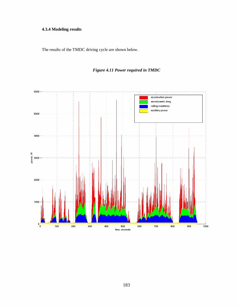
4.3.4 Modeling results
The results of the TMDC driving cycle are shown below.
Figure 4.11 Power required in TMDC

184
Acceleration power demands the greatest peaks in the cycle, and also accounts for most of the
energy in the cycle (not including braking energy recovered from negative accelerations). Rolling
resistance accounts for somewhat less energy, and aerodynamic drag even less. The 60 W of
auxiliary power is at most 10% of the average power.
Interestingly, the average power is approximately one tenth of the maximum power. The extreme
variability in the power demands suggests that hybridization would be useful, with a battery
providing surges of extra power during bursts of acceleration and also the capability to store
braking energy.
The physical model shows that the power needed, under the TMDC, is an average 566 W of electric
power out of the fuel cell without parasitics. A complete analysis of fuel economy, however,
requires a polarization curve of efficiency versus net power, and an understanding of the parasitic
power. This is in section 4.5.
4.3.4.1 Battery powered scooter
The parasitic power requirements of the fuel cell have not yet been calculated but there is enough
information here to calculate performance of a scooter running on just a single battery. The power
output is the same as the fuel cell power output except without the parasitic requirement. A total of
4.1 kWh (output) are needed to store enough electricity for 200 km of range.

185
Table 4.8: Taiwan battery-powered scooter performance
TMDCdriving cycle
30 km/hcruising
Average speed 19.3 km/h 30 km/h
Average power (electric output) 566 W 615 W
Mileage in terms ofelectric output
35.5 km per kWh-output
48.8 km perkWh-output
Maximum power output 5.6 kW 615 W
Total energy storage for 200 km at 30 km/h 4.1 kWh
The battery requirements, given the different USABC battery technology predictions and a 4.1 kWh
storage capacity, are compared to today’s lead-acid batteries.
Table 4.9: Various battery-powered designs for Taiwan scooter
Lead-acid: today’s battery
Mid-Term advanced battery
Long-Termadvanced battery
Weight 117 kg 62 kg 25 kg
Volume 58 L 36 L 16 L
Cost $245-$735(current)
$735(mid-term)
$490(long-term)
For the lead-acid battery, the critical assumptions were 35 Wh/kg and 70 Wh/L. Note that in the
mid-term and long-term cases, the battery weight and volume are determined by the maximum
energy requirement, not the power requirement. In fact, a mid-term battery of this size would offer
7.7 kW of maximum power, while the long-term battery would output a maximum of 8.2 kW! The
limiting factor in battery size and weight for these batteries is energy storage, not power storage.
Section 4.7 on hybrid design shows how decoupling the energy and power functions of the battery
improve the system.

186
Today’s ZES-2000 scooter with far shorter range than the systems described above gives an idea of
how much room is available in the scooter: at least 44 kg and 15 L (not including the electric motor
and controller). The next step is to design a fuel cell power system within these size and weight
parameters that can output a continuous 610 W for 30 km/h cruising for 200 km (or 6.7 hours);
produce a 5.6 kW maximum output; and generate 3.2 kW of continuous hill climbing power.
4.4 Fuel Cell System Design and Integration
4.4.1 Design tradeoffs
The fuel cell stack is specified by only two independent variables plus the polarization curve and the
maximum power:
1. Maximum power
2. The polarization curve
3. Power density
4. Number of cells in the stack
(Note that, instead of power density and number of cells, we could have equivalently chosen area
per cell and total active area of all cells)

187
powervoltage
0.0
0.1
0.2
0.3
0.4
0.5
0.6
0.7
0.8
0.9
1.0
volta
ge (
V)
0
100
200
300
400
500
600
700
800
900
1000
pow
er d
ensi
ty (
mW
/cm
^2)
0 200 400 600 800 1000 1200 1400 1600 current density (mA/cm^2)
4.4.1.1 Maximum power and the polarization curve
A maximum gross fuel cell power of 5.9 kW is assumed from parasitic requirements calculated in
section 4.4.5. This is slightly over the sum of the maximum TMDC requirement of 5.6 kW net
power plus an initial estimate of 300 W for parasitic power losses. The parasitic requirements are
discussed in greater detail later on, but for now it is enough to say that they are approximately linear
with gross power output so that maximum parasitic power occurs at maximum gross power.
The polarization curves used are those derived from Energy Partners for single atmospheric-
pressure cells; these are extrapolated to be equal to future stack performance.
Figure 4.12 Polarization curve
Data is from Barbir is for a single cell running on hydrogen/air, with a GoreMEA and operating temperature of 60(C. Air-side stoichiometry is 2.5.26

188
4.4.1.2 Power density
The first choice to make is to determine the power density to operate at, under conditions of
maximum power. If maximum output is arranged to take place at low power density, the left portion
of the polarization curve is used (since power density scales almost linearly with current density);
voltage, and thus efficiency, are high in this portion of the curve. However, a large total active fuel
cell area is needed and much electrolyte membrane and platinum will then be required. The stack
size will be larger.
If a low total area is used, then power density per area is high. The power density curve peaks at
high current densities, with correspondingly low voltages and low efficiencies. (The low total area
can be achieved by a combination of low cell area and/or few cells). Total price is a monotonic
function of total area, so the high power density approach results in a smaller stack and cheaper
stack, although efficiency would suffer and consequently hydrogen storage requirements for a given
range would be higher.
Power density also controls the flow rates of the air and hydrogen reactants. The flow rates are
functions of the designed hydrogen utilization and oxygen stoichiometric ratio, and also of the
efficiency of the fuel cell; low efficiency means that more reactants must be flowed for a given
power output. Thus, for a given power level, high power densities mean higher flow rates because
they operate in the low voltage (low efficiency) portion of the polarization curve. The sizes and
costs of air management equipment are determined in part by flow rate, but it should be noted that
the scooter application demands flow rates far below those normally available for vehicle systems so
most systems for scooters based on automotive designs would be oversized anyway.

189
To maximize efficiency and produce a small, cheap fuel cell, a high power density is selected.
According to the polarization curves presented, power is maximized at about 1300 mA•cm-2; to be
conservative and leave room for unusual bursts of speed, a point below this power peak is chosen:
1000 mA•cm-2. At 1000 mA•cm-2, voltage is 0.614 V, and power density is thus 614 mW•cm-2. For
5.9 kW at this point, 9.6 x 103 cm2 of active area are needed.
4.4.1.3 Number of cells
The number of cells is a function of the desired operating voltage. The electric scooter industry in
Taiwan is standardizing on 48 V electric motors, so the number of cells is chosen so that the stack
operates in the vicinity of 48 V at the most common power demand; note that in a fuel cell, as the
total power output changes, the voltage varies as well.
The DC-to-DC conversion is assumed to be performed by the motor controller, and is included in
the 77% drivetrain efficiency. (In comparison, standalone DC-to-DC converters from Vicor offer
approximately 410 W/L and 381 W/kg, with efficiencies of 80%-90%; prices are on the order of 1
$/W.27,28) All parasitic power – fans, pumps, blowers, etc. – should be DC to avoid the large
additional expense of a DC-to-AC inverter.
The average TMDC power demand is 566 W, and later modeling in shows that the final result
including parasitic power (after iterative calculation) is 674 W. With a 9.6x103 cm2 total membrane
area, the power density is 70 mW•cm-2. To obtain this power density on the polarization curve, 79
mA•cm-2 and 0.870 V are needed - only 8% of the maximum current density, and high up on the
efficiency curve. The system is designed to run at 48 V at this point, and dividing 48 V by the 0.870
V per cell gives a minimum of 56 cells. Area per cell is then approximately 170 cm2.
190
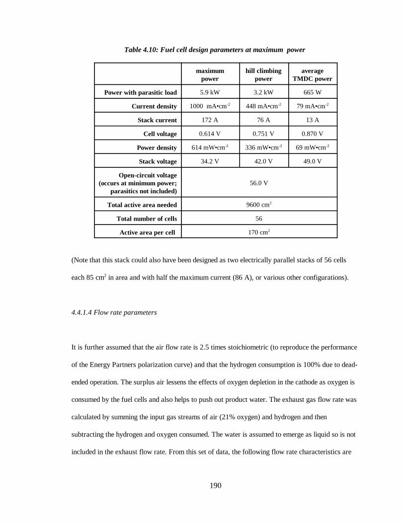
Table 4.10: Fuel cell design parameters at maximum power
maximumpower
hill climbingpower
averageTMDC power
Power with parasitic load 5.9 kW 3.2 kW 665 W
Current density 1000 mA•cm-2 448 mA•cm-2 79 mA•cm-2
Stack current 172 A 76 A 13 A
Cell voltage 0.614 V 0.751 V 0.870 V
Power density 614 mW•cm-2 336 mW•cm-2 69 mW•cm-2
Stack voltage 34.2 V 42.0 V 49.0 V
Open-circuit voltage(occurs at minimum power;
parasitics not included)56.0 V
Total active area needed 9600 cm2
Total number of cells 56
Active area per cell 170 cm2
(Note that this stack could also have been designed as two electrically parallel stacks of 56 cells
each 85 cm2 in area and with half the maximum current (86 A), or various other configurations).
4.4.1.4 Flow rate parameters
It is further assumed that the air flow rate is 2.5 times stoichiometric (to reproduce the performance
of the Energy Partners polarization curve) and that the hydrogen consumption is 100% due to dead-
ended operation. The surplus air lessens the effects of oxygen depletion in the cathode as oxygen is
consumed by the fuel cells and also helps to push out product water. The exhaust gas flow rate was
calculated by summing the input gas streams of air (21% oxygen) and hydrogen and then
subtracting the hydrogen and oxygen consumed. The water is assumed to emerge as liquid so is not
included in the exhaust flow rate. From this set of data, the following flow rate characteristics are

191
derived:
Table 4.11: Flow rate parameters at maximum power
volumetric molar mass
hydrogen intake rate 2.6 CFM 0.05 mol•s-1 0.1 g•s-1
air intake rate 15.6 CFM 0.30 mol•s-1 8.6 g•s-1
total exhaust gas rate 16.9 CFM 0.27 mol•s-1 7.8 g•s-1
(liquid) waterproduction rate
0.9 mL•s-1 0.05 mol•s-1 0.9 g•s-1
4.4.2 Gas subsystem
As discussed previously, the pressure drop in fuel cell stacks has been estimated at 0.5 - 2 psi. With
a 50% blower efficiency, worst-case 2 psi air drop, and the calculated 15.6 cfm of air flow, this is a
maximum theoretical power consumption of 200 W. In theory, this scales down linearly with
decreasing flow rate, but in practice the pressure drop also decreases as a function of flow rate so
the decrease is somewhat sharper than linear. A heavy-duty blower that could be used to provide the
required output is the Ametek 5.7" BLDC three-stage blower, model 116638-08. Its volume flow
capacity is much higher than the 16 cfm required, but it is the smallest model capable of the
relatively high 2 psi needed.29 Retail cost is $430.
The blower power was modeled in the simulation as a linear 50-250 W load, for a gross power
output of 50-5850 W. This is a conservative calculation based on comparison with a reported
parasitic power draw of 105 W for a 24 VDC Ametek blower at 1.3 psi for a 4 kW nominal power
fuel cell.30
On the hydrogen side, a pressure regulator expands the hydrogen from either the 1-10 atm partial

192
pressure of a metal hydride system, or a 3600 psi (260 atm) pressure of a compressed gas system.
4.4.3 Water subsystem
A low fuel cell operating temperature of 50(C is chosen to minimize evaporation losses and
eliminate the need for external humidification (and complex control of that humidification). The
maximum allowable fuel cell temperature is set to 65(C.
According to Mazda Demio documentation, external humidification requires an additional 15% in
stack volume, but thin wicking polymer membranes can allow water to be backdiffused from the
cathode to the anode to keep the membranes humidified without external humidification.31 The
wicking polymers could alternately transfer water from a reservoir to pre-humidify incoming air if
humidification turns out to be necessary after all.
4.4.4 Cooling subsystem
There are several heat flows to consider in fuel cell systems.
1. Waste heat must be removed from the stack with a liquid coolant loop.
2. The liquid coolant must have heat removed at the cold side with a fan.
3. Air entering the system may be preheated in order to retain more water from any humidification
4. The humidification water, if any, can be preheated as well
5. Reformers, if present, require temperatures of at least 300(C to operate, and may produce net
heat
6. Heat must be supplied to the metal hydride system, if one exists, in order to desorb the hydrogen.

193
To optimize the system, some of the flows can be combined. For example, the coolant loop is a
convenient source of heat for a metal hydride storage system, while the blower could be designed to
draw its input air from behind the coolant radiator.
All heat flows in the system are functions of the instantaneous power, since the waste heat,
hydrogen demand, and air demand all scale according to the efficiency curve with respect to power
in almost the same way. The maximum heating load occurs at maximum power in the driving cycle
- at 5.9 kW of gross electric output, efficiency is 41.2% and heat output is 8.4 kW. However, the
average heat load during typical TMDC driving is much lower, only 742 W. Given sufficient
thermal mass, temperatures in the stack can be kept near the design point without the use of a large
radiator. The ultimate concern is to keep the temperature low to avoid evaporating too much water
from the membrane.
In comparison, a 20% efficient 5 kW internal combustion engine outputs 20 kW of waste heat. The
difference is that this load is produced at high temperatures and thus is easily rejected to the
environs by air blowing over cooling fins
There are two beneficial cooling effects that are not quantified here. First, fuel cell efficiency is
calculated on a higher heating value basis, meaning that the product water is assumed to emerge
solely as liquid water. In fact, some is vaporized and this removes heat from the system, making the
cooling design somewhat conservative.32
Second, some heat is “used up” by the intake air. At a maximum flow rate of 8.6 g/s, an intake
temperature of 30(C, and a heat capacity for air of approximately 1 J•g-1•K-1, 170 W of heat are
required if the incoming air heats up to the stack temperature of 50(C. This small amount of cooling

194
is not included below but is noted for the sake of completeness.
4.4.4.1 Cooling from storage system
Here, cooling from metal hydride adsorption is discussed, along with more conventional cooling.
The temperature of the fuel cell stack is modeled over the entire driving cycle to ensure that the fuel
cell remains within its designed limits of 50(C and 65(C.
TiFe metal hydride systems consume 28 kJ of heat per mole of hydrogen desorbed. In the system,
the maximum heat production is 8.4 kW and occurs at the maximum gross power of 5.9 kW. Here,
hydrogen consumption is 0.05 moles•s-1, so the hydride takes up 1.4 kW (16.7%) of the waste heat.
This percentage increases as the fuel cell is turned down to lower powers, because the number of
moles of hydrogen per heat output increases due to the greater efficiency; over the full range, the
metal hydride system eliminates 16.7% - 30.2% of the waste heat. This reduces the size of the
radiator and decreases the parasitic power required for cooling.

195
average hill climbing maximum
gross waste heatnet waste heat
TiFe hydride cooling0
1000
2000
3000
4000
5000
6000
7000
8000
9000
heat
or
pow
er (
W)
0 1000 2000 3000 4000 5000 6000 net power (W)
Figure 4.13 Metal hydride cooling vs. power
For this reason, metal hydrides have a significant advantage over gas cylinders. Combining a water
cooling system for the fuel cell with the metal hydride allows the transfer of this heat, although a
backup heating system might be necessary for startup heating and active control of the metal
hydride temperature. This backup system could be a resistance heater wrapped around part of the
metal hydride, connected to the startup battery. (The pressure of hydrogen gas over the hydride at
room temperature would be greater than atmospheric, so there would be some hydrogen at startup.
However, with waste heat slow to reach the hydride, an extra heater could provide a faster flow rate
for immediate high power).

196
4.4.4.2. Active cooling
There are several possibilities for liquid cooling.
1. Cooling is provided by a closed loop water coolant circulated at constant flow rate through the
stack by way of cooling plates. The hot water exiting the stack is circulated to a heat exchanger
exposed to the atmosphere, where a fan enhances heat transfer. The fan speed can be increased to
provide additional cooling. Alternately, a constant-speed fan can be used in a thermostat mode
(allowed to switch on and off as needed), allowing the coolant temperature to fluctuate.
2. Variable coolant flow rate, fixed fan speed. As stack output power increases, the coolant
circulation speed is increased. The change in temperature of coolant as a function of power is
dependent on the heat exchanger properties. A variable-flow pump is needed.
3. Variable coolant flow rate, variable fan speed.
4. The pump is eliminated, reducing weight, cost, and parasitic power; instead, a refrigerant
designed to boil at the fuel cell operating temperature is used in conjunction with a check valve, and
the expanding gas drives circulation in the coolant loop.
In all cases, water circulation should be stopped altogether when the engine is warming up to
operating temperature, so some kind of thermostat (if not variable) control should be employed for
the coolant loop.
The heat exchanger cooling factor, in terms of watts of heat dissipated per degree of temperature
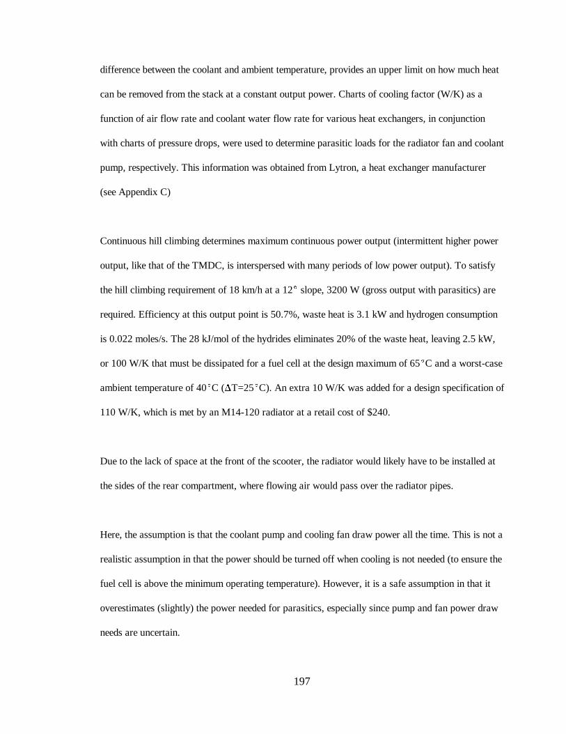
197
difference between the coolant and ambient temperature, provides an upper limit on how much heat
can be removed from the stack at a constant output power. Charts of cooling factor (W/K) as a
function of air flow rate and coolant water flow rate for various heat exchangers, in conjunction
with charts of pressure drops, were used to determine parasitic loads for the radiator fan and coolant
pump, respectively. This information was obtained from Lytron, a heat exchanger manufacturer
(see Appendix C)
Continuous hill climbing determines maximum continuous power output (intermittent higher power
output, like that of the TMDC, is interspersed with many periods of low power output). To satisfy
the hill climbing requirement of 18 km/h at a 12( slope, 3200 W (gross output with parasitics) are
required. Efficiency at this output point is 50.7%, waste heat is 3.1 kW and hydrogen consumption
is 0.022 moles/s. The 28 kJ/mol of the hydrides eliminates 20% of the waste heat, leaving 2.5 kW,
or 100 W/K that must be dissipated for a fuel cell at the design maximum of 65(C and a worst-case
ambient temperature of 40(C (�T=25(C). An extra 10 W/K was added for a design specification of
110 W/K, which is met by an M14-120 radiator at a retail cost of $240.
Due to the lack of space at the front of the scooter, the radiator would likely have to be installed at
the sides of the rear compartment, where flowing air would pass over the radiator pipes.
Here, the assumption is that the coolant pump and cooling fan draw power all the time. This is not a
realistic assumption in that the power should be turned off when cooling is not needed (to ensure the
fuel cell is above the minimum operating temperature). However, it is a safe assumption in that it
overestimates (slightly) the power needed for parasitics, especially since pump and fan power draw
needs are uncertain.

198
4.4.4.3. Heat generation under the TMDC
Maximum heat dissipation is determined by continuous hill climbing, but to ensure that the short
spikes of high heat generation in the TMDC do not push the fuel cell temperature past 65(C, the
temperature of the stack was simulated using a simple model. Heat generation under the TMDC
simulation has the same general shape as the power output graph, but the peaks and valleys are
exaggerated because efficiency decreases with increasing power output.
Figure 4.14 Heat generation as a function of time in TMDC

199
∆T Q
M C M Cτ=
+
�
1 1 2 2
Note that average heat generated is 742 W for the 5.9 kW stack. After the metal hydride heat
absorption is included, this decreases to an average load of only 393 W. The net heat generated was
calculated for each step of the TMDC and used to calculate a change in temperature for the stack.
The purpose of this further test was to make sure that the cooling factor (sized for continuous load)
would be enough to keep stack temperature below the design limit of 65(C through the peaks and
spikes of the TMDC.
The heat capacity equation used was
Q = M C T ∆
for heat Q, stack mass M, average heat capacity T, and change in temperature �T. This was
discretized for each time step, and the mass and heat capacity were separated into the different
materials found in the stack, resulting in the following equation:
is the heat power generated in a given time interval; M is the mass of the parts of the stack that�Q
make up the bulk of the total weight and are closest to the membranes (i.e. “1" for the stainless steel
separator plates and “2" for the polypropylene gaskets); C is the heat capacity of the stack
materials; and - is the length of time of a single time step of the model.

200
Table 4.12 Stack temperature model parameters
parameter value note
Mass of 316 stainless steel separator plates
2.0 kg 0.5 J•g-1•(C-1 specific heat capacity
Mass of polypropylene gaskets 0.8 kg 2 J•g-1•(C-1 specific heat capacity
Heat capacity of stack as a unit 2.6 kJ•(C-1 Weighted sum of steel and polypropylene
Specific heat capacity of stack 0.93 J•g-1•(C-1 c.f. water at 4.2 J•g-1•K
Heat exchanger cooling factor 150 W•K-1 maximum cooling
Ambient temperature 40(C worst case
Heat removed by metal hydride 28 kJ•mol H2-1 minimum 17% of waste heat
The assumption made was that most of the heat would be trapped inside the plastic housing
(designed for electrical insulation), removed mainly by the active cooling system. The membrane
itself is negligible because it is so light. This simple model does not include the effects of heat
conductivity - just heat capacity.
The cooling system was designed to turn on only above a temperature of 50(C in the stack (as
detected by thermistors in the stack), with a maximum allowable temperature of 65(C. The
following temperature patterns were recorded for the TMDC for cooling factors of 110 W/K as
designed, and 30 W/K for comparison.

201
Figure 4.15 Stack temperature as a function of time in TMDC
The smaller cooling factor is perfectly adequate to keep the maximum temperature below 65(C but,
as calculated previously, the full 110 W/K is needed for sustained hill climbing.
As discussed, either the cooling fan or the pump could be switched on and off to produce cooling. In
practice, the pump should be the unit controlled, because some cooling is still derived from pumping
the water through the externally-exposed radiator, even if the fan blowing over the radiator is off.
This seems like a benefit, except that excessive cooling would lower the fuel cell stack temperature
below its designed operating point of 50(C; also, when the fuel cell is first started, it needs to warm
up as quickly as possible.

202
A more sophisticated temperature simulation would include a time lag between the temperature
measurement inside the stack and the control (turning the pump on or off). A more sophisticated
design would vary the pump speed in order to reduce the power taken up by the pump, especially
since adequate control could be maintained at just 20 W/K to achieve the result graphed above. This
would decrease parasitic load and extend range, but, again, this was not assumed here due to the
uncertainty in actual cooling power needs.
4.4.4.4 Selection
To achieve the upper limit of 110 W•K-1, a Lytron M14-120 radiator was selected. The cooling
system includes a metal heat exchanger, pump operating at 1 gallon per minute (0.06 L/s), and fan
blowing over the heat exchanger. For 110 W•K-1 of cooling, a fan speed of 375 cubic feet per
minute (cfm) is necessary.33
According to performance charts (Appendix C), the coolant pressure drop in the radiator is 1.0 psi,
while the fan-blown air decreases in pressure by 0.16 inches of water (40 Pa). Assuming a 50%
pump efficiency and 50% fan efficiency, these translate into power demands of 25 W for the pump
and 14 W for the fan. (Note that this takes the 1.0 psi coolant water pressure drop in the radiator
and adds an estimated 2 psi drop from the fuel cell cooling cell flow fields)
It might seem that air supplied by ram-effect from the motion of the scooter would be enough to
cool the exchanger. This is true in most cases, making the heat exchanger fan speed conservative,
but false for the case of low-speed hill climbing, where power demands are high but air speed low.
The design is also conservative because parasitic power is calculated as if the pump were on all the
time, whereas this is actually not true as discussed previously.

203
This heat exchanger weighs 8.9 kg and takes up 15.2 L of space, including the fan, and accounts for
a significant fraction of the total weight and volume.
4.4.5. Overall parasitics
Note that the specifications for pumps and blowers and radiators are for industrial, and often
stationary, AC power components. This was done to get an idea of real world performance and cost
without designing specifically for the scooter application. In practice, DC components would be
needed to avoid an expensive DC-to-AC inverter, and components could likely be optimized for the
application at hand. Prices, described in Chapter 5, are retail; cost to the scooter manufacturer
would be as little as a quarter of retail.
The system requires a blower to push the air in, but omits the bulkier compressor and possibility of
expander motor power recovery at the exhaust of the fuel cell.
The maximum parasitics estimated for the scooter system are 25 W for the coolant pump and 14 W
for the fan blowing over the radiator, as discussed previously, plus a power draw from the Ametek
blower power which is assumed to scale linearly with flow rate (i.e. power), from a minimum of 50
W of power at no load to 200 W at maximum fuel cell output of 6 kW. The power is calculated as
if the pump and fan were on all the time, with the blower always requiring 50 W, for a total
parasitic load of 89 W – 239 W over the output range of the fuel cell; in practice, power is saved by
turning off – or slowing down – the fan and pump when not used.
The results are compared with those obtained by a study published by the Schatz Energy Research
Center.34 The Schatz report calculates the following total parasitic power requirements for a

204
linear estimate ofparasitic powerpresented here
Schatz parasiticpower
50
100
150
200
250
300
350
frac
tion
of g
ross
pow
er
0 1000 2000 3000 4000 5000 6000
net power (W)
nominal 4 kW vehicle (“Personal Utility Vehicle” - i.e. golf cart) fuel cell stack operating at
atmospheric pressure.
In the Schatz system, the parasitic power comes from the water coolant pump, atmospheric-pressure
blower, and the cooling fans. The system operates at approximately 40(C, and the air flow rate at
1.74 kW is 4.48 cfm (approximately 60% higher at the same power than the system presented here).
So parasitic demands vary from 100% of gross power down to 5% above 2000 W, a fairly small
fraction.
Figure 4.16 Parasitics as a function of power
The next graph compares power usage as a percentage of gross power for both systems.

205
Schatzparasitic power
linear estimate ofparasitic powerpresented here
0%
10%
20%
30%
40%
50%
60%
70%
80%
90%
100%
frac
tion
of g
ross
pow
er
0 1000 2000 3000 4000 5000 6000
net power (W)
Figure 4.17 Parasitics as a percentage of power
Finally, the parasitic power reduction is represented as a voltage reduction in the polarization curve.
The result is a combined efficiency that has net electricity output as its numerator. The peak
efficiency point is shifted to higher current densities and efficiency is reduced below 50% at all
points.

206
gross efficiency
net efficiencywith parasitics
net power
0%
20%
40%
60%
80%
100%
effic
ienc
y
0
2
4
6
8
10
net p
ower
(kW
)
0 1000 2000 3000 4000 5000 6000
gross power (W)
Figure 4.18 Effect of parasitics on efficiency
4.5 Integrated Model
4.5.1 System performance
The complete model takes the vehicle physical model described at the beginning of this chapter, and
integrates the efficiency of the motor/controller subsystem, parasitic power demands, and the fuel
cell polarization curve to determine overall efficiency: the amount of hydrogen consumed for a given
travel distance under both the Taipei Motorcycle Driving Cycle and steady state 30 km/h driving
conditions. The overall performance is used to identify the sizing of subcomponents like the fuel

207
storage supply and thus to determine the overall system weight and size.
Essentially, the driving cycle model is run, and at each discrete point in time, the power needed at
the wheels is calculated and divided by the 77% drivetrain efficiency. An auxiliary power
component of 60 W is added. Parasitic power is determined as a function of this total, and added.
(This is an iterative process because the parasitic power is included in the total power, from which
the parasitic power is calculated.)
Next, this total electrical output power is divided by the efficiency at that power demand; this
efficiency is determined from the voltage on the polarization curve for the power required. The
result is the amount of hydrogen consumed at the time interval, in terms of higher heating value
energy units.
The results, over the driving cycle, are the maximum and average power (including parasitics); and
the fuel economy in terms of hydrogen consumed per kilometer traveled. The latter is readily
converted to miles per gallon of gasoline equivalent. An overall efficiency is calculated for the
conversion process.
A battery-powered option is considered using the same basic model, but with no parasitic power to
consider because fans, blowers, and pumps are not needed.
As before, the total scooter curb weight was set at 130 kg, and a 75 kg driver was added. Later
results show that the vehicle weight is approximately the same as this assumption.

208
Table 4.13 System Performance under TMDC and at cruising speed
TMDC 30 km/h cruise
Maximum power from fuel cell(includes drivetrain and parasitics)
5.91 kW 725 W
Average fuel cell output power 674 W 725 W
Overall efficiency 46.7% 58.5%
Fuel economy relative to hydrogen 0.527 km/g H2 0.807 km/g
Equivalent “on-vehicle” fuel economy 344 mpge 522 mpge
Hydrogen storage for 200 km range 380 g 248 g
Average output power without parasitics(battery powered scooter)
566 W 614 W
Fuel economy of battery powered scooter 35.5 km/kWh 48.8 km/kWh
Battery energy storage for 200 km range 6.5 kWh 4.1 kWh
Note that these battery energies are given in terms of total energy output. The energy that must be
put into these batteries is higher due to less-than-100% charging and discharging efficiency.
However, this additional energy is not included here because price and performance figures for the
zinc-air batteries are given in terms of energy output.
4.5.2 Size and weight of power system
The detailed analysis done in Appendix B and described in section 3.1.3.3 estimates a stack size and
volume of 7.6 kg and 7.8 L respectively. This is a power density of 0.78 kW/kg and 0.76 kW/L for
the stack alone, slightly less than 1996 Ballard stacks at 1 kW/L.
Assuming a factor of two extra for air and heat and water management subsystems gives power
densities of 0.39 kW/kg and 0.38 kW/L. (The PNGV Technical Roadmap requirements are 0.4
kW/kg and 0.4 kW/L.35) That is a simple estimate;; the following paragraphs produce a more

209
detailed analysis of the subsystems. First, the heaviest and bulkiest subcomponents are analyzed and
listed in Table 4.14. These are the blower that supplies air to the fuel cell stack, the pump that
circulates cooling air, and the radiator. Prices are projected for mass production, with more details
in section 5.1.3.
Table 4.14 Subcomponent summary
Brand ModelDimensions
(in cm) Size WeightCost
(long term)
Fuel cell stack – – – 7.8 L 7.6 kg $220
Starter battery Yuasa GRTYT4L-BS
11 x 7 x 9 0.7 L 1.3 kg $10
Coolant pump generic – 8 x 12 x 12 1.2 L 1 kg $20
Radiator with fan Lytron M14-120 15.2 L 8.9 kg $60
Blower Ametek 116638-08 15 diameterx 17 length
2.9 L 2.7 kg $110
plumbing, wiring, etc.
generic – – 2.0 L 3.0 kg $50
coolant water – – – – 0.64 kg* –
TOTAL STACKWITH AUXILIARIES
– – – 29.8 L 24.6 kg $470
The “generic” pump has pressure requirements of 2.5 psi and apumping flow rate of 1 gallon per minute. This is adequately suppliedby an aquarium-type pump. Electric cabling, air manifolds, waterplumbing were estimated to add 3 kg and 2 L and a cost of $100
*Note that the radiator holds 320 mL of water when full, and with anestimated total of twice that amount of water in the entire system, thisadds an additional 0.64 kg of weight.
The total performance figures for the stack with auxiliaries are 0.24 kW/kg and 0.20 kW/L. The
stack proper takes up 27% of the mass and 26% of the volume.
In comparison, the overall fuel cell stack weight of the Schatz 4 kW system described previously
was 75 lbs or 34 kg; the entire power system weighed 200 lbs or 90 kg. Stack volume was 10" x

210
11" x 21", or 39 L.36 With the greater room of a golf cart, engineering for minimum volume is not
so critical, but these results still indicate that reduced size and weight have not yet been
demonstrated
The sizes and weights with the hydrogen storage system included are listed in Table 4.15 below.
Both a current Ergenics metal hydride system and predicted FeTi performance are included, along
with a Dynetek cylinder and the ZES-2000 battery-powered scooter for comparison purposes.37
Table 4.15 Size of various storage designs
storage systemenergy stored
range at 30 km/h
(km)
rangeunder
TMDC(km)
energy storage(battery or H 2)
complete drive system
weight volume weight volume
ZES-2000lead-acid batteries
1.34kWh
60 40* 44 kg 15 L 60 kg 24 L
DTI TiFe hydride 250 g H2 200 132 21 kg 4 L 61 kg 43 L
Ergenics hydride(aluminum body)
204 g H2 165 108 27 kg 14 L 67 kg 53 L
Dynetek cylinder(compressed gas)
350 g H2 282 184 11 kg 31 L 51 kg 70 L
“complete drive system” refers to the motor and controller from Table2.2 (15.5 kg and 9.1 L together), the fuel cell stack, auxiliaries, andhydrogen storage.
* Note that the ZES-2000 can not actually sustain the TMDC, as itlacks the power necessary for the high-speed accelerations; its range isgiven as if it had could produce the required maximum power using itscurrent batteries. For comparison, according to an unspecified patternof “urban driving”, it is listed at a range of approximately 30 km;reported data shows that it reaches 80 km on a single completedischarge at 30 km/h.38
Also, although the ZES-2000 does not actually use the UniqueMobility motor / controller system specified, these numbers are similarto those of other motor/controller systems and were used in calculatingtotal size and weight for the battery-powered scooters.

211
This comparison has used the criteria of size and weight, but it should also be noted that cooling
loads are higher for compressed gas hydrogen storage systems, due to the lack of desorption
cooling. This results in larger cooling loads and higher parasitic demands from the cooling system,
not shown here. The results of Table 4.15 are discussed in the subsection following.
4.5.3 Evaluation
Average two-stroke scooters weigh 70 kg and up, but the overall ZES-2000 prototype mass is 105
kg. A Honda CUV-ES electric scooter weighs 130 kg. Fuel cell powered scooters would weigh
about as much as the CUV-ES; recall that one of the concerns in the consumer satisfaction survey
was the extra weight of the electric scooter. While this might remain an item of difficulty in terms of
handling while the system is off, the extra performance provided by the 6 kW fuel cell system
partially compensates for the high mass.
The fuel cell vehicle offers more than three times the range of the ZES-2000, with roughly the same
weight of drive system. The fuel cell systems requires 18 to 36 additional liters of storage space
over that of the ZES-2000. There is a helmet storage chamber in the design that could be
commandeered for additional fuel storage; this is approximately 10-15 L of space. Additional
volume would have to come from a redesigning of the scooter body to make more room available,
but note that current electric scooters already use redesigned large-capacity bodies.
Current laboratory-scale metal hydrides, as exhibited by the Ergenics system, are almost 30 L larger
than the ZES-2000 power system, so progress must be made in improving metal hydride technology.
The following charts describe the breakdown of size and weight for the various subsystems, for a

212
FC stack (10.9%)
TiFe storage (34.8%)
auxiliaries (29.1%)
motor/controller (25.2%)
FC stack (18.3%)
motor/controller (21.4%)
TiFe storage (8.7%)
auxiliaries (51.6%)
FeTi hydrogen storage system
Figure 4.19 Weights of subsystems
Figure 4.20 Volumes of subsystems
A subsequent chapter deals with the costs of the various systems, but the next section is a
discussion of whether operating the fuel cell at higher pressures (with consequent greater efficiency)
might improve performance and reduce the size of the fuel cell required.

213
P n V dP nR TP
Pad iab aticP
P
= =−
−
∫
−
� �
1
2
111
2
1γγ
γγ
4.6 Pressurized fuel cell option
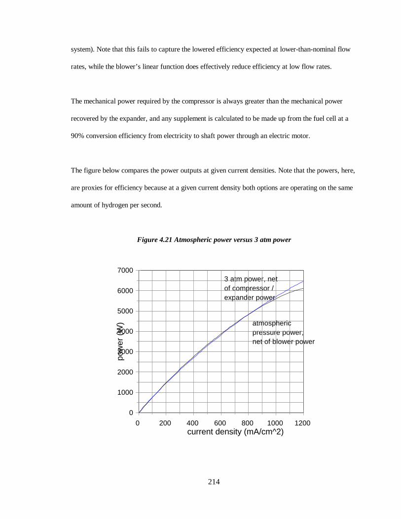
One of the two options considered for improving the performance of the base design was to operate
the fuel cell above atmospheric pressure. To quantify this benefit, the higher voltage output
obtainable was compared to the additional power needed to drive the compressor. Also included was
the fact that a turbine running of the fuel cell exhaust would reduce the compressor load.
Calculations were based on a adiabatic, non-isentropic system with the 68% efficiency assumed
previously.
Power out for an adiabatic expander (or compressor):
is the flow rate in moles•s-1; R is universal ideal gas constant, 8.314 J·mol-1·K-1. The specific heat�n
ratio � is the ratio of Cp to Cv for the working fluid. Assumptions: the intake air is an ideal gas
consisting of nitrogen and 20.95% oxygen; the exhaust (mainly nitrogen, with some water vapour
and unused hydrogen) is an ideal gas with the stoichiometric amount of oxygen removed by the fuel
cell reaction, and no water vapour.
The benefit of compression is calculated using the two Energy Partners polarization curves
discussed previously (3 atm and atmospheric). The atmospheric power is net of blower parasitic
power, which is a linear function from 50 W to 250 W over the 5.9 kW operating range of the fuel
cell stack. The pressurized stack power is net of compressor and expander powers, as calculated for
a 68% efficiency expander and 68% efficient compressor. (same as the DOE’s projected automotive
214
3 atm power, netof compressor /expander power
atmosphericpressure power,net of blower power
0
1000
2000
3000
4000
5000
6000
7000
pow
er (
W)
0 200 400 600 800 1000 1200 current density (mA/cm^2)
system). Note that this fails to capture the lowered efficiency expected at lower-than-nominal flow
rates, while the blower’s linear function does effectively reduce efficiency at low flow rates.
The mechanical power required by the compressor is always greater than the mechanical power
recovered by the expander, and any supplement is calculated to be made up from the fuel cell at a
90% conversion efficiency from electricity to shaft power through an electric motor.
The figure below compares the power outputs at given current densities. Note that the powers, here,
are proxies for efficiency because at a given current density both options are operating on the same
amount of hydrogen per second.
Figure 4.21 Atmospheric power versus 3 atm power

215
The difference expands to 350 W at 1200 A•cm-2, so the pressurized fuel cell does have benefits at
high pressure. However, at the maximum operating point of 1000 A•cm-2, the advantage of the 3
atm fuel cell is only 105 W, or 1.8% of the gross power. Although there is an unquantified benefit
for the pressurized fuel cell due to the lesser need for humidification and easier water removal, the
gain is quite limited and the scooter cannot accept the additional cost and weight of an additional
turbocompressor system. Also, unlike the case for automobiles, the fuel cell stack size would not be
appreciably reduced by operating at 3 atm.
If the DOE goals of 3 kg and 4 L for a turbocompressor can be realized, and efficiency is good at
the under-10 g/s flow rates required in scooters, then the slight performance benefit will be worth a
small price premium.
4.7 Hybrid option design
A second optimizing option was considered. Due to the extremely irregular nature of scooter
driving, with average power only 8% of maximum power, peaking power provided by a secondary
power device might be an efficient way to reduce the fuel cell size. The fuel cell would provide
baseload power and charge up the secondary (peaking) power source for later use. A peaking power
device, which could be an advanced high-power battery, an ultracapacitor, or a flywheel, would also
enable regenerative braking.
The targets of hybridization, for the scooter are to:

216
1. Reduce system cost by reducing fuel cell size; peaking power batteries are cheaper than
additional fuel cell capacity, at least for the next several years.
2. Increase total fuel economy with regenerative braking and lower curb weight. For the same
hydrogen storage, greater fuel economy means greater range.
3. Improve vehicle handling by reducing curb weight.
The major drawback is that hybrid systems require more complex controls and power conditioning
systems. To optimize the system, a balance must be struck between secondary power source size
and main power source size. An important consideration is whether weight and volume of
auxiliaries will decrease significantly if a smaller fuel cell is used.
4.7.1. Types of hybrids
There are several types of hybrid vehicle designs. Most of these are defined for internal combustion
engines and used for the purposes of (i) increasing engine efficiency, (ii) reducing emissions, and
(iii) reducing cost if the main engine is expensive, like a fuel cell. Hybrids are divided into parallel
and series systems.
For a combustion hybrid, a parallel system allows both the engine and the peaking battery (via
electric motor) to drive the wheels using two separate systems. This system is more mechanically
complex due to the two driveshaft attachments, but allows simultaneous use of the battery and the
combustion engine.

217
In contrast, a series hybrid routes all power electrically. The combustion engine drives a generator
(not required in the parallel version), which can supply energy to the wheels and the peaking battery.
Output from the generator and the peaking battery go to the wheels. Generally, the engine can be set
to operate only at its most efficient speed, recharging the battery as needed and avoiding transients
which might produce more emissions.
The more specific operating policies listed below are from the DOE HEV program guidelines.39 The
word “battery” is used interchangeably with “secondary energy storage system,” although this
system could actually be a flywheel or ultracapacitor.
1. Thermostat series. The vehicle is run on battery power by default, with the primary power source
activated (at the optimum power level) when the battery drops below a predefined minimum. The
primary power source acts as a thermostat, turning on and off to maintain battery state of charge.
This policy allows the primary power source to run at its peak efficiency point.
2. Electric-assist parallel. The primary source provides power by default, and the battery is
discharged only in high-power situations. The battery is recharged by regenerative braking, but in
the case of combustion engine hybrids, cannot be recharged by the engine because there is no
generator. The primary power source can be sized below the maximum power required since it is
assisted by the battery.
3. Primary power-assist parallel. Identical to the previous system, but with the battery providing
power, and the internal combustion engine supplying peaking power. Very similar to a “range-
extender” system in that the battery functions as the main energy storage device.

218
4. Load-leveler series. The average power is matched to the output of the primary power source,
while logic attempts to maintain the state of charge of the battery at a predefined medium level.
Peaking power is supplied by the battery, but the primary power source load is allowed to vary as
well to maintain the state of charge of the battery. (This contrasts with the thermostat series option,
where the combustion engine stays at its optimal point).
The different policies show that the design is motivated by a desire to keep the combustion engine at
its optimum point (maximizing fuel economy and minimizing emissions) for the series options, and
reducing the engine size in the parallel options.
A fuel cell hybrid is technically a series hybrid because there is a single drive system (electric). The
fact that all power is electric means that, if designed properly, the control logic can allow both fuel
cell and battery to drive the wheels (like an electric-assist parallel), or let the fuel cell recharge the
battery (like a load-leveler series). Several axes of optimization remain - for example, how large to
make the fuel cell, when to use the battery and when to recharge it, and how large to make the
battery.
4.7.2. Fuel cell sizing
In order to calculate how to divide the power needs between the fuel cell and the battery, two criteria
were specified. First, maximum power (5.6 kW net of parasitics) had be sustained for at least ten
seconds. Users would be very disappointed to find that, after a few seconds of pushing their scooters
to the maximum output, power started to fall off because the battery was used up. Second, the
scooter had to sustain - indefinitely - the slope-climbing requirements. In other words, it had to
generate enough power to climb a 12( slope at 18 km/h.

219
The physical model showed that these results can be obtained with a fuel cell stack with a maximum
output of 3.2 kW gross power (3.0 kW net). Total cell active area was reduced by reducing the area
of each cell to 110 cm2, while the number of cells was kept the same in order to retain the 48 V
motor voltage. To reach the maximum power output level thus required the addition of a 2.6 kW
peaking battery. This is the first hybrid scooter case.
One other case was considered. This one is targets the short term where fuel cells are extremely
expensive and the fuel cell size must be minimized at all costs: a fuel cell sized to output only 1.0
kW of net power (1.1 kW gross power), with a large battery for the remaining 4.6 kW.
This scooter would not be capable of indefinitely sustaining hill climbing as specified at the
beginning of the chapter. The specified performances can only be achieved for under three minutes
until the batteries drain down to their 20% limit, and the continuously sustained hill climbing speeds
are lower than the requirements, as shown in the table below.
Table 4.16 Hybrid 1.1 kW scooter inadequacies
15(( slope 12(( slope
Required performance 10 km/h 18 km/h
Limited amount of time atthis speed as battery is drained
140 s 70 s
Limited distance at this speed 380 m 360 m
Sustainable maximum speed(after battery depleted; fuel cell only) 4.7 km/h 5.8 km/h
Cooling load is significant in hybrid vehicle design as well as in the original pure fuel cell design;
again, the critical situation is hill climbing requiring 3.2 kW of continuous output. In the 5.9 kW
full-sized fuel cell, continuous operation at 3.2 kW gross output takes place at 51% efficiency, and

220
heat production is consequently low. A 3.2 kW maximum power fuel cell, however, is only at 43%
efficiency when it is continuously operated at 3.2 kW, producing more heat. The greater heat also
necessitates higher pump and fan loads for the radiator, meaning greater parasitic loads.
Parasitic power loads were calculated with an iterative process. The first step was to estimate a
parasitic load. Then the maximum gross output power including parasitics was calculated for hill
climbing. A maximum heat output was then solved, and the parasitic power required to sustain this
cooling load was calculated. The process was repeated until the results converged. In the example
here, after the results had settled down to stable values, the following results were obtained:
For the first hybrid, the maximum load was 3020 W, with parasitic power costs of 66 W for pump
and fan, and 50-250 W for the blower depending on load. The total fuel cell output was 3205 W at
this net power output, for a waste heat load of 4240 W. With hydride cooling at 17.2% at this
hydrogen flow rate, the remaining heat load was 3510 W, or 140 W/K at the pre-defined �T of
25(C, which was supplied by fans and pumps with the total of 66 W.
The 1.1 kW system was easier to solve because the output was simply capped at 1.0 kW of net
output, because no attempt had to be made to find the total power at which the hill climbing
requirements could be met. A smaller M10-080 radiator was used. Under maximum conditions of
1.1 kW gross power, heat generation was 1430 W, or 1180 W after metal hydride desorption, for a
cooling load of 47 W/K.

221
Table 4.17 Hybrid fuel cell stack designs
Pure FC Hybrid 1 Hybrid 2
Maximum gross power 5.9 kW 3.2 kW 1.1 kW
Stack current at maximum power 172 A 89 A 31 A
Efficiency at maximum current density 41.2% 43.2% 43.6%
Total active area needed 9600 cm2 5600 cm2 2000 cm2
Total number of fuel cells 56 56 56
Active area per cell 170 cm2 100 cm2 35 cm2
Maximum fuel cell heat generation 8.4 kW 4.2 kW 1.4 kW
Maximum heat generation(after metal hydride cooling)
7.0 kW 3.5 kW 1.2 kW
Cooling factor needed at maximum power (��T=25((C)
280 W/K 140 W/K 47 W/K
Maximum net fuel cell power 5.9 kW 3.0 kW 1.0 kW
Battery power needed – 2.6 kW 4.6 kW
4.7.3 Peaking battery and operating policy
The peaking power battery model is described in section 2.2.3.1 and has the following properties.
Note that the specific power and power density are much higher for the battery than the fuel cells
(see Table 4.24), so that hybridization makes sense in reducing total weight and volume.
Table 4.18 Peaking power battery characteristics
Specific power at 43 second discharge 836 W/kg
Specific energy 17 Wh/kg
Power density by volume 853 W/L
Energy density by volume 17 Wh/L
The heat generated by the battery is not included in the system modeling. It is on the order of 10%

222
of the output power, low compared to the fuel cell. At maximum output power (4.6 kW for the 1.1
kW stack hybrid) this could be almost 500 W in addition to the fuel cell, but this heat load is
infrequently reached. The operating policy of the battery is defined as follows.
1. The state of charge of the battery is allowed to vary between 80% and 20% over the driving
cycle. The state of charge is kept away from these “hard limits” in order to reduce the risk of large
excusrions (overcharging or draining to zero), either of which could permanently damage the
battery.
2. The state of charge is set at the beginning of the driving cycle is set to 50%
3. The battery is activated (discharged) whenever the fuel cell maximum power is not enough for the
driving cycle power plus auxiliary and parasitic loads, and makes up the entire difference.
4. Regenerating always recharges the battery as long as the maximum charging current is not
exceeded, up to the 80% limit
5. The battery is charged up from the fuel cell at a specified rate whenever (i) the state of charge
dips below 55% and (ii) power demand at that instant is less than 400 W. The charging rate is equal
to 400 W minus the instantaneous power demand from the wheels, auxiliaries, and parasitics.
4.7.4 Simulation results
First, fuel economy was determined under steady-state, 30 km/h driving conditions.

223
Table 4.19 Hybrid performance at 30 km/h
Parameters5.9 kW pure FC
3.2 kWhybrid
1.1 kWhybrid
fuel cell conversion efficiency 58.5% 56.4% 50.0%
average fuel cell output power 725 W 751 W 710 W
fuel economy in terms of hydrogen 0.807 km/g 0.751 km/g 0.703 km/g
“on-vehicle” fuel economy 522 mpge 486 mpge 455 mpge
change from pure FC – -4% -15%
hydrogen for 200 km 248 g 266 g 284 g
Efficiency decreased as the fuel cell size decreased, because the smaller fuel cells were operating
closer to their maximum output. For the results below, the hydrogen storage system was scaled
linearly to keep range at 200 km. The driving cycle was more interesting because its decelerations
created the possibility of regenerative braking.
Table. 4.20 Hybrid performance under TMDC
Parameter5.9 kWpure FC
3.2 kWhybrid
1.1 kWhybrid
Fuel cell maximum power 5.91 kW 3.24 kW 1.11 kW
Battery maximum power needed – 2.61 kW 4.63 kW
Average total power output,battery + fuel cell
674 W 709 W 726 W
Average fuel cell power 674 W 698 W 577 W
Fuel economy (mpge) 344 316 343
Change in fuel economy – -8.2% -0.3%
Overall conversion efficiency 56% 53% 47%
Braking energy absorbed – 62 kJ 82 kJ
Average power absorbed – 65 W 86 W
Braking energy recovered as a fractionof theoretical maximum braking losses
– 51% 68%

224
The 1.1 kW fuel cell puts out 100 watts less average power than the 5.9 kW fuel cell, because the
86 W (average) that is recovered from regenerative braking can supplement the peaks. However,
conversion efficiency from hydrogen heating value to electricity is lower at 47%, because the fuel
cell is operating more frequently near its maximum power (minimum efficiency). More hydrogen
must be used to produce the 577 W of power than if the larger, pure fuel cell were used with the
same batteries. The result is a net fuel economy that is the same as the pure fuel cell.
The 3.2 kW hybrid actually consumes more power in the TMDC due to the higher parasitic losses,
and for the same reason of operation near maximum power given above.
The regenerated fractions of 51% and 68% are close to the 70% theoretical maximum that can be
regenerated. The differences are due to the limiting maximum charging rate and the fact the at some
points the battery is already full when regenerative braking is possible. In terms of total power,
though, these figures are equivalent to 9% – 14% of the total fuel cell output.

225
Figure 4.22 Division of power between fuel cell and battery during TMDC, 3.2 kW stack
In this diagram, the dark area above the horizontal line represents theenergy supplied by the peaking power battery, while the light gray areabelow the line is the energy supplied by the fuel cell. The same schemeis used in Figure 4.24.

226
Figure 4.23 State of charge of battery over TMDC, 3.2 kW stack
The careful observer will note that battery energy does not return to initial levels over the driving
cycle - in fact, there is a net gain from regeneration of 58.3 kJ, or an average of 60 W over the 950
second cycle. There is a not insignificant amount of surplus energy that could be applied to the
wheels, if the battery were employed using a more sophisticated policy (for example, using the
battery even if power demand is not greater than the maximum fuel cell output), and fuel economy
would be slightly improved.

227
Since the object was to minimize component cost and not necessarily produce the maximum
mileage, the design of more efficient hybrid strategies will have to await future studies.
Figure 4.24 Division of power between fuel cell and battery during TMDC, 1.1 kW stack

228
Figure 4.25 State of charge of battery over TMDC, 1.1 kW stack
4.7.5 Hybrid power system designs
The subsystem performance requirements and sizes/weights are listed for the two hybrid designs,
with the base pure fuel cell system for comparison.

229
Table 4.21 Hybrid system design
Parameter5.9 kWpure FC
3.2 kWhybrid
1.1 kWhybrid
Maximum hydrogen flow rate 2.6 cfm 1.4 cfm 0.5 cfm
Maximum air flow rate 15.6 cfm 8.1 cfm 2.8 cfm
Worst-case cooling requirement 110 W/K 150 W/K 50 W/K
Cooling fan power requirement 14 W 28 W 4 W
Coolant pump power requirement 25 W 38 W 21 W
Fuel cell stack weight 6.7 kg 5.4 kg 4.1 kg
Fuel cell stack size 7.8 L 5.3 L 3.2 L
Fuel cell cost (manufacturing cost) $220 $160 $140
Battery maximum power needed – 2.6 kW 4.6 kW
Battery weight – 3.1 kg 5.6 kg
Battery size – 3.0 L 5.4 L
Battery cost (retail) – $195 $340
The same DTI model was used to calculate fuel cell stack sizes, weights, and costs. The designs are
described in greater detail below.
4.7.5.1 Design for 3.2 kW fuel cell
For the 3.2 kW fuel cell, fuel economy actually goes down with hybridization. There are three
reasons: (i) the cooling system parasitic load is larger (ii) the fuel cell is operating more frequently
near its maximum load (iii) the battery is rarely used to output energy.
At maximum cooling load and 50% efficiency, the cooling fan runs at 500 cfm (0.24 inches of water
pressure drop) and uses 28 W of power while the pump pushes coolant at 1 gpm (2.5 psi pressure
drop) and uses 38 W. Thus, the base load power needed for the cooling system is 66 W.

230
The lower air intake flow requirements might make a smaller and cheaper blower feasible.
With auxiliaries the power system totals are 21.9 kg and 26.6 L, for power densities of 0.15 W/kg
and 0.12 W/L.
Table 4.22 Component breakdown for 3.2 kW scooter
Component Weight Volume Long-term cost
Fuel cell stack 5.4 kg 5.3 L $165
Radiator and fan 8.9 kg 15.2 L $60
Coolant pump 1.0 kg 1.2 L $10
Blower 2.7 kg 2.9 L $110
plumbing, wiring, etc.
2.0 kg 2.0 L $50
coolant water 0.9 kg – –
peaking power battery 3.1 kg 3.0 L $195
TOTAL STACKWITH AUXILIARIES
25.1 kg 29.6 L $590
motor 11.4 kg 5.0 L $125
controller 4.1 kg 4.1 L $150
hydride for 266 grams H2 22.8 kg 4.0 L $200
TOTAL DRIVE SYSTEM 63 kg 43 L $1065
Due to the lower fuel economy of the 3.2 kW system at 30 km/h, slightly more metal hydride is
needed: 266 grams for 200 km. This requires a 22.8 kg system taking up 4.0 L of space.
The total size and weight are very close to the original, 5.9 kW fuel cell. Mainly this is because the
subsystem sizes remain the same even though the fuel cell proper becomes smaller. Smaller blowers
and coolant pumps could be used, reducing weight slightly, but the largest subcomponent (the
radiator) has to stay large in order to handle the higher cooling factor of 140 W/K.

231
4.7.5.2. Design for 1.1 kW fuel cell
In the second hybrid, the battery is used much more often and contributes frequently to the total
power output. However, for the same reason, the battery must be frequently replenished, and due to
the small size of the 1.1 kW fuel cell, the fuel cell often runs near its inefficient maximum output.
The net fuel economy is almost identical to that of the pure fuel cell.
Cooling is different. The system is sized for cooling when it is running flat out at the maximum 1
kW of net output, rather than for sustained (3020 W) hill climbing. After metal hydride cooling, the
worst-case cooling load is less than 50 W/K. This is achievable with a fan at 140 cfm with 0.125
inches of water air pressure drop (4 W of power), and a pump at 1 gallon per minute with 0.5 psi
water pressure drop (21 W of power), for a total of 25 W. The lower cooling load of 50 W/K means
that a smaller radiator can be used here – the Lytron M10-080.
With auxiliaries, the power system totals are 21.9 kg and 26.6 L, for power densities of 0.15 W/kg
and 0.12 W/L.

232
Table 4.22 Component breakdown for 1.1 kW scooter
Component Weight Volume Long-term cost
Fuel cell stack 4.1 kg 3.2 L $135
Radiator and fan 3.1 kg 2.3 L $30
Coolant pump 1.0 kg 1.2 L $10
Blower 2.7 kg 2.9 L $110
plumbing, wiring, etc. 2.0 kg 2.0 L $50
coolant water 0.6 kg – –
peaking power battery 3.1 kg 3.0 L $340
TOTAL STACKWITH AUXILIARIES
20.1 kg 17.0 L $675
motor 11.4 kg 5.0 L $125
controller 4.1 kg 4.1 L $150
hydride for 285 grams H2 24.3 kg 4.3 L $215
TOTAL DRIVE SYSTEM 60 kg 30 L $1165
Due to the lower fuel economy of the 1.1 kW system at 30 km/h, slightly more metal hydride is
needed: 284 grams for 200 km. This requires a 24.3 kg system taking up 4.2 L of space.
The extra battery size is compensated for by the smaller fuel cell, while the smaller radiator makes a
large difference in reducing the total volume.
4.7.5.3 Hybrid zinc-air scooters
If fuel cells can be hybridized with peaking power batteries, why not battery powered scooters?
Regenerative braking would extend the range of the vehicle, while separating the power and energy
functions might allow a smaller, less expensive power system. In the fuel cell, energy and power are
decoupled. The fuel cell engine is sized for a maximum power output, and the amount of hydrogen

233
carried can be varied to meet range requirements. With the battery, a larger power necessarily
corresponds to a larger energy storage, and sizing for power may result in overdesigned energy (or
vice versa). The hybrid battery system reduces this dependence by using batteries with two different
power-to-energy relationships.
The hybrid battery design presented here uses zinc-air batteries (high energy density) for range, plus
the peaking power lead-acid batteries (high power density) described above. The two sets of
batteries operate in the same way as the fuel cell hybrid, so that the peaking power of the high
power lead-acid batteries can be added to the zinc-air baseload battery’s power, and the peaking
batteries can be used to absorb regenerative braking energy.
The power and energy requirements are specified so that the scooter has enough power to sustain
the maximum accelerations of the TMDC, and enough energy to drive 200 km at a constant speed
of 30 km/h (or 145 km under the TMDC). 5.6 kW of output power and 4.1 kWh of energy storage
are needed, and the following results are obtained:
Table 4.24: Hybrid battery configuration for Taiwan scooter model
ParameterZinc-Air
baseload batterySpiral lead-acidpeaking battery Total
Weight 20.5 kg 4.5 kg 25.0 kg
Energy Capacity 4.1 kWh 0.07 kWh 4.1 kWh
Peak Power 1.8 kW 3.8 kW 5.6 kW
Specific Energy 200 Wh/kg 17 Wh/kg 168 Wh/kg
Specific Power 90 W/kg 836 W/kg 210 W/kg
Volume 27.1 L 4.4 L 31.5 L
Long term mass-production price
80 $/kWh 75 $/kW –
Total price $330 $285 $615

234
The zinc-air volumetric energy density is calculated to be 150 Wh/L from published data; cost for
high-power lead acid battery is estimated at 166 $/kW based on a scaled up version of Bolder
batteries.40 This is reduced to 75 $/kW in mass production (The Rebel battery’s density is
approximately 1 kg/L and the future goal is $150/kWh for long term USABC batteries and
advanced lead-acid batteries. Somewhat arbitrarily, power systems are assumed to be half as
expensive per kilowatt as base load batteries.41)
Note that the continuous power output of 1.8 kW is not sufficient for the continuous hill climbing
needs; rather, the baseload battery is sized for the 200 km range and 4.1 kWh required. Thus, the
hybrid battery vehicle is more comparable to the 1.1 kW fuel cell system than the 3.2 kW system.
(The Electric Fuel company has its own, more conservative hybrid battery scooter theoretical
design; it is specified for 4 kW maximum power and 3.0 kWh energy storage, for a claimed range of
200 km. This 3.0 kWh storage is underspecified, according to the calculations earlier in this
chapter. Their power source consists of two 8 kg zinc-air batteries, each 9.9 L, 7.5 kg, and with an
output of a maximum of 0.75 kW. The peaking power source must thus supply 2.5 kW, and is not
described in the Electric Fuel report although it likely will be a NiCd battery.42
4.7.6 Hybrid results
The hybridization study reveals that peaking power batteries do not significantly reduce the mass
and volume of the fuel cell system, because the auxiliary cooling and fluid management systems
require a certain minimum space and mass which does not decrease rapidly with size.
Fuel economy did not improve significantly, due to the fact that with a 3.2 kW fuel cell, only a few

235
excursions required use of the battery and parasitic loads were higher than for the pure fuel cell.
The 1.1 kW version produced fuel economies equal to the original pure fuel cell because of its lower
efficiencies; on the other hand, it reduced the size of the fuel cell stack by a factor of more than five,
which is important for the short term cost.
Table 4.25 Hybrid power system summary
5.9 kW fuel cell
3.2 kWhybrid
1.1 kWhybrid
1.8 kW battery hybrid
ultimate stack cost $244 $161 $124 –
stack cost/kW $42 $47 $103 –
stack size 7.8 L 5.3 L 3.2 L –
stack weight 7.6 kg 5.4 kg 4.0 kg –
stack with auxiliaries, size (excl. peaking battery)
29.8 L 26.6 L 11.6 L –
stack with auxiliaries, weight(excl. peaking battery)
24.6 kg 21.9 kg 14.6 kg –
baseload battery (zinc-air) volume
– – – 27.1 L
baseload battery (zinc-air) weight
– – – 25.0 kg
power sourcepower density
0.20 kW/L 0.12 kW/L 0.09 kW/L 0.07 kW/L
power sourcespecific power
0.24 kW/kg 0.15 kW/kg 0.08 kW/kg 0.07 kW/kg
In terms of the useful performance measurements of fuel economy total power system size/weight
(including fuel cell or baseload battery, peaking power battery, and hydrogen storage, but not motor
and controller), the following results are obtained:

236
Table 4.26 Performance metrics
5.9 kW fuel cell
3.2 kWhybrid
1.1 kWhybrid
1.8 kW batteryhybrid
hydrogen storage (FeTi hydride)weight for 200 km range
21.4 kg 22.8 kg 24.3 kg –
hydrogen storage(FeTi hydride) volume
3.7 L 4.0 L 4.3 L –
peaking power battery weight – 3.1 kg 5.6 kg 4.5 kg
peaking power battery size – 3.0 L 5.5 L 4.4 L
total drive system weight 61 kg 63 kg 60 kg 45 kg
total drive system size 43 L 43 L 30 L 41 L
30 km/h fuel consumption 0.807 km/g 0.751 km/g 0.703 km/g 48.8 km/kWh
TMDC fuel consumption 0.527 km/g 0.484 km/g 0.525 km/g 36.2 km/kWh
30 km/h fuel economy 522 mpge 486 mpge 455 mpge 1053 mpge
TMDC fuel economy 344 mpge 320 mpge 363 mpge 780 mpge
Range at 30 km/h 200 km 200 km 200 km 200 km
Range under TMDC 131 km 129 km 149 km 148 km
“total drive system” includes fuel cell and hydrogen storage, or zinc-air battery; motor / controller; peaking power battery. Costs arediscussed in the next chapter.
Note that the ZES drive system weight is 44 kg of lead-acid batteries plus 15.5 kg of motor and
controller (assuming similar characteristics as the UQM motor/controller). This is about 60 kg, the
same as the fuel cell systems.
System size does not decrease significantly with hybridization except in the case of the 1.1 kW
hybrid where much lower cooling requirements mean a much smaller radiator. The smaller fuel cell
weight is roughly compensated for by the added weight of the batteries, and the larger hydrogen
storage tank. TMDC performance is better for the 1.1 kW hybrid because the frequent decelerations
allow regenerative braking gains; the same is true for the 1.8 kW battery hybrid.

237
On the other hand, certain other factors decrease more or less linearly with fuel cell size, foremost
among them membrane area and platinum cost. Significant cost reductions might be possible under
such a system for the near future while fuel cells remain extremely expensive; unfortunately, these
costs are not reflected in the price calculations above, which rely upon ultimate price estimates for
mass-produced stacks.
More complex hybrid operation policies could be used to try to better predict power demands; these
would optimize battery usage by controlling more cleverly when to recharge, how quickly to
recharge, and the state of charge to maintain in the battery.
4.7.7 Near-term possibilities
To compare these designs with what is available today, portable stacks from H-Power and Ballard
were inserted into the 1 kW fuel cell design. A single PS-250 fuel cell unit commercially available
from H Power produces 250 W net power, weighs 10.3 kg, and has a volume of 16 L.43 This does
not include storage. (The system is air-cooled, and with the correct geometry this could be possible
for a scooter version) The existing design can actually output 330 W; to be conservative, retail units
are sold derated to 250 W. Using three units to supply the 1.0 kW net output desired produces a
power system weight of 31 kg and volume of 48 L. Currently costs are on the order of $6,000 for a
unit like the PS-250, with mass-production costs expected to drop to $1,000.44 For the required
three, then, the current cost would be on the order of $18,000 and $3,000 in the long run.
On the other hand, Ballard Power Systems has developed a 1 kW (net power) stack that weighs 18
kg and has a volume of 33 L including all packaging.45
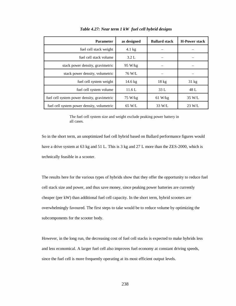
238
Table 4.27: Near term 1 kW fuel cell hybrid designs
Parameter as designed Ballard stack H-Power stack
fuel cell stack weight 4.1 kg – –
fuel cell stack volume 3.2 L – –
stack power density, gravimetric 95 W/kg – –
stack power density, volumetric 76 W/L – –
fuel cell system weight 14.6 kg 18 kg 31 kg
fuel cell system volume 11.6 L 33 L 48 L
fuel cell system power density, gravimetric 75 W/kg 61 W/kg 35 W/L
fuel cell system power density, volumetric 65 W/L 33 W/L 23 W/L
The fuel cell system size and weight exclude peaking power battery inall cases.
So in the short term, an unoptimized fuel cell hybrid based on Ballard performance figures would
have a drive system at 63 kg and 51 L. This is 3 kg and 27 L more than the ZES-2000, which is
technically feasible in a scooter.
The results here for the various types of hybrids show that they offer the opportunity to reduce fuel
cell stack size and power, and thus save money, since peaking power batteries are currently
cheaper (per kW) than additional fuel cell capacity. In the short term, hybrid scooters are
overwhelmingly favoured. The first steps to take would be to reduce volume by optimizing the
subcomponents for the scooter body.
However, in the long run, the decreasing cost of fuel cell stacks is expected to make hybrids less
and less economical. A larger fuel cell also improves fuel economy at constant driving speeds,
since the fuel cell is more frequently operating at its most efficient output levels.

239
1. Jet P. H. Shu, Wei-Li Chiang, Bing-Ming Lin, Ming-Chou Cheng. Mechanical Industry ResearchLaboratories, Industrial Technology Research Institute. “The Development of the Electric PropulsionSystem for the ZES2000 in Taiwan”. (Date unknown; not the same as the SAE paper in reference 7, eventhough it appears to be written by the same authors. October 1997 or later.)
2. Yoshihiro Nakazawa, Chiaki Humagai, Mikio Kato. “Development of an electric scooter for practicaluse” in JSAE Review 15 (1994) 373-377
3. Chien-Tung Liu, Bing-Ming Lin, Jyh-Sheng Pan. “Design and development of a zero-emission scooterfor Taiwan” in Journal of Power Sources 59 (1996) 185-187
4. Peter A. Lehman, Charles E. Chamberlin. “Design and Performance of SERC’s Fuel Cell PoweredVehicle Fleet” in Fuel Cell Seminar Abstracts 1998. 714-717
5. Mowick Limited Golf & Leisure Vehicles. “E-Z Go 4Caddy” http://www.mowick.com/ezwhite.htmAccessed July 30, 1999
6. Chien-Tung Liu, C. C. Kuo, Jyh-Sheng Pan, Bing-Ming Lin. “Development of electric motor cycletechnologies in Taiwan” J. Power Sources 48 (1994) p. 244
7. P. H. Jet Shu, Wei-Li Chiang, Bing-Ming Lin, Ming-Chou Cheng. “The Development of the ElectricPropulsion System for the Zero Emission Scooter in Taiwan”. (1997) SAE 972107
8. ibid
9. Highway Tire Committee, SAE. Revised by the Rolling Resistance Subcommittee. “Measurement ofPassenger Car, Light truck and highway truck and bus tire rolling resistance” (March 1997) SAEInformation Report J1270. Section 8.1
10. Frank Rowland Whitt, David Gordon Wilson. Bicycling Science (MIT Press: Cambridge, 1974) p. 93
11.Wei-Li Chiang, Power Machinery Division Director, ITRI-MIRL (Industrial Technology ResearchInstitute, Mechanical Industry Research Laboratories. Personal communication, September 11 1998
12. CALSTART web site. “DARPA Consortia EV and Hybrid EV Technology Projects - (PNGV) TargetAttributes” http://www.calstart.org/about/pngv/pngv-ta.html
13. Energy and Environment Analysis. “Analysis of Fuel Economy Boundary for 2010 and Comparison toPrototypes” (November 1990) Prepared for Martin Marietta Energy Systems, Contract No. 11X-SB0824.
A calculation of costs, both for the scooter and for the fuel it uses, is found in the next chapter.
Infrastructure and overall fuel economy are also discussed.
References for Chapter 4

240
p. 4-11.
14. M. Ross and W. Wu. “Fuel Economy Analysis for a Hybrid Concept Car Based on a Buffered Fuel-Engine Operating at a Single Point” SAE Paper 950958, presented at the SAE International Exposition,Detroit, MI, February 27 - March 2 1995
15. C. E. (Sandy) Thomas, Brian D. James, Frank Lomax, Ira F. Kuhn, Jr. Directed Technologies,Inc.“Integrated Analysis of Hydrogen Passenger Vehicle Transportation Pathways”, draft final report. ForNREL, subcontract AXE-6-16685-01. March 1998. p. 61
16. Bernward E. Bayer, “Motorcycles”. Chapter 10 of Aerodynamics of Road Vehicles. Fourth Edition.Ed. Wolf-Heinrich Hucho. p. 502
17. Arne LaVen. “Driving Cycle Analysis of the Sun ComTM Battery Electric Scooter” (November 1998)Desert Research Institute. p. 26
18. Wei-Li Chiang, Power Machinery Division Director, ITRI-MIRL. Personal communication,September 11 1998
19. Owner’s manual for Honda CH250 Elite250 1986, (Honda Motor Company: 1985) p. 68
20. T. C. Pong, personal communication. October 29, 1998.
21. Arne LaVen. Energy and Environmental Engineering Center, Desert Research Institute. “DrivingCycle Analysis of the Sun ComTM Battery Electric Scooter” November 1998
22. Chien-Tung Liu, Bing-Ming Lin, Jyh-Sheng Pan. p. 186
23. Toshiharu Sawada, Minoru Wada, Masanori Noguchi, Buhei Kobayashi. Komatsu Zenoah Co.“Development of a Low Emission Two-Stroke Cycle Engine” SAE 980761 (1998)
24. C.T. Liu, C. C. Kuo, J. S. Pan, B. M. Lin.“Development of electric motor cycle technologies inTaiwan”
25. Christopher S. Weaver, Lit-Mian Chan.“Motorcycle Emission Standards and Emission ControlTechnology” Revised Final Report, submitted to The World Bank. (Engine, Fuel, and EmissionsEngineering, Inc.: August 1994) page v.
26. Frano Barbir. Energy Partners. “Operating Pressure and Efficiency of Automotive Fuel Cell Systems”No date. 1997 or later.
27. Vicor product data sheet. “The MegaPAC family” http://www.vicr.com/pdf/ds_megapac.pdf AccessedJuly 9, 1999
28. Vicor sales representative. Personal communication. July 14 1999.
29. Lisa Fawcett, AMETEK. Personal communication. April 26 1999.
30. Charles Chamberlin, Schatz Energy Research Center, Personal communication. May 20 1999
31. Mazda Australia web page. “Mazda”. http://www.mazda.com.au/corpora/460.htm. Accessed June 17,1999

241
32. If the entire 0.9 g/s were vaporized (with a latent heat of vaporization of 2.2 kJ/g for 100(C water)approximately 2 kW of cooling would be realized, or about 25% of the total heat generated.
33. Lytron product catalog, “Standard OEM Coils” at http://www.lytron.com/catalog/oemframe.htm. Lastaccessed April 11, 1999
34. Charles E. Chamberlin and Peter A. Lehman. “Design and Performance of SERC’s Prototype FuelCell Powered Vehicle”
35. National Research Council. Review of the Research Program of the Partnership for a New Generationof Vehicles. Second Report (National Academy Press, Washington: 1996) p. 53
36.Susan Ornelas, Research Engineer, Schatz Energy Research Center. Personal communication February17 1999.
37. No similar size and weight data was available for the CUV-ES scooter. Also, the Dynetek cylinder isone that holds about 40% more hydrogen than the DTI model, as no Dynetek cylinder currently exists forthe designed 250 gram size.
38. Jet P. H. Shu et al, “The Development of the Electric Propulsion System for the ZES2000 in Taiwan”
39. Department of Energy Hybrid Electric Vehicle Program. “Energy Management and System Control”.http://www.hev.doe.gov/components/energman.html. Accessed May 10, 1999.
40. Bolder “Rebel” battery pack product sheet; see specifications in section 2.2.3.1
41. ALABC [Advanced Lead-Acid Battery Consortium] web site. “About ALABC”http://www.alabc.org/about.html
42. Jonathan Whartman, Ian Brown. Electric Fuel, Ltd. “Zinc Air Battery-Battery Hybrid for PoweringElectric Scooters and Electric Buses” November 1, 1998
43. Rene Dubois, H Power. Personal communication June 7 1999
44. Arthur Kaufman, H Power, personal communication May 21 1999
45. Ballard product data sheet. “1 kW fuel cell generator”