chapter radar measurements - mers -- byu - news & · pdf file18.10 coordinate systems ......

POMR-720001 book ISBN : 9781891121524 February 9, 2010 16:55 1

C H A P T E R

18Radar Measurements

W. Dale Blair, Mark A. Richards, David A. Long

�

�

�

�

Chapter Outline

18.1 Introduction . . . . . . . . . . . . . . . . . . . . . . . . . . . . . . . . . . . . . . . . . . . . . . . . . . . . . . . . . . . . . . . . . . . . . 1

18.2 Precision and Accuracy in Radar Measurements . . . . . . . . . . . . . . . . . . . . . . . . . . . . . . . . 2

18.3 Radar Signal Model . . . . . . . . . . . . . . . . . . . . . . . . . . . . . . . . . . . . . . . . . . . . . . . . . . . . . . . . . . . . . 7

18.4 Parameter Estimation . . . . . . . . . . . . . . . . . . . . . . . . . . . . . . . . . . . . . . . . . . . . . . . . . . . . . . . . . . . 9

18.5 Range Measurements . . . . . . . . . . . . . . . . . . . . . . . . . . . . . . . . . . . . . . . . . . . . . . . . . . . . . . . . . . . 14

18.6 Phase Measurement . . . . . . . . . . . . . . . . . . . . . . . . . . . . . . . . . . . . . . . . . . . . . . . . . . . . . . . . . . . . 19

18.7 Doppler and Range Rate Measurmements . . . . . . . . . . . . . . . . . . . . . . . . . . . . . . . . . . . . . . 20

18.8 RCS Estimation . . . . . . . . . . . . . . . . . . . . . . . . . . . . . . . . . . . . . . . . . . . . . . . . . . . . . . . . . . . . . . . . . 24

18.9 Angle Measurements . . . . . . . . . . . . . . . . . . . . . . . . . . . . . . . . . . . . . . . . . . . . . . . . . . . . . . . . . . . 25

18.10 Coordinate Systems . . . . . . . . . . . . . . . . . . . . . . . . . . . . . . . . . . . . . . . . . . . . . . . . . . . . . . . . . . . . 34

18.11 Further Reading . . . . . . . . . . . . . . . . . . . . . . . . . . . . . . . . . . . . . . . . . . . . . . . . . . . . . . . . . . . . . . . . 35

18.12 References . . . . . . . . . . . . . . . . . . . . . . . . . . . . . . . . . . . . . . . . . . . . . . . . . . . . . . . . . . . . . . . . . . . . . 35

18.13 Problems . . . . . . . . . . . . . . . . . . . . . . . . . . . . . . . . . . . . . . . . . . . . . . . . . . . . . . . . . . . . . . . . . . . . . . . 36

18.1 INTRODUCTION

A radar is designed to transmit electromagnetic energy in a format that permits the extrac-tion of information about the target from its echo. Once a target is detected, the next goalis often to precisely locate that target in three-dimensional space, which requires accuratemeasurements of the distance and angle (both azimuth and elevation) to the target. Inaddition, it is often desirable to estimate the radar cross section (RCS) and radial velocityof the target as well.

There are major differences in the way these quantities are measured. The range tothe target is measured by estimating the two-way time delay of the transmitted signal.The radial velocity or range rate of the target is measured by estimating the Doppler shiftin the echo signals. The angular position of the target is measured by comparing signalstrength in multiple simultaneous antenna beams offset in angle from one another, obtainedeither with an antenna structure that forms multiple offset beams (e.g., monopulse) or byscanning a single beam across or around the target (e.g., conical scan). A radar measuresthe RCS by using a propagation model (radar range equation) with the measured rangeand transmitted and received pulse powers to deduce the RCS.

1

long

Cross-Out

long

Replacement Text

G


2 C H A P T E R 18 Radar Measurements

The basic radar range, angle, and radial velocity measurements previously discussedare usually made repeatedly and then combined through kinematic state estimation orfiltering of the measurements to produce improved three-dimensional position, velocity,and acceleration estimates, a process called tracking the target. The procedures that com-bine the individual measurements are called track filtering algorithms. For closely spacedobjects, radar resolution and issues of data association play important roles in the kine-matic state estimation, as detections may result from reflected energy from multiple targetsand clutter, thermal noise, electromagnetic interference (EMI), and jamming signals fromelectronic attack sources. Chapter 19 considers how the measurements are combined inthe track filtering process.

In this chapter, some of the common techniques for radar measurements are described,along with factors determining their accuracy and precision. Space limitations precludeconsidering additional techniques and error sources.

18.2 PRECISION AND ACCURACYIN RADAR MEASUREMENTS

18.2.1 Precision and Accuracy

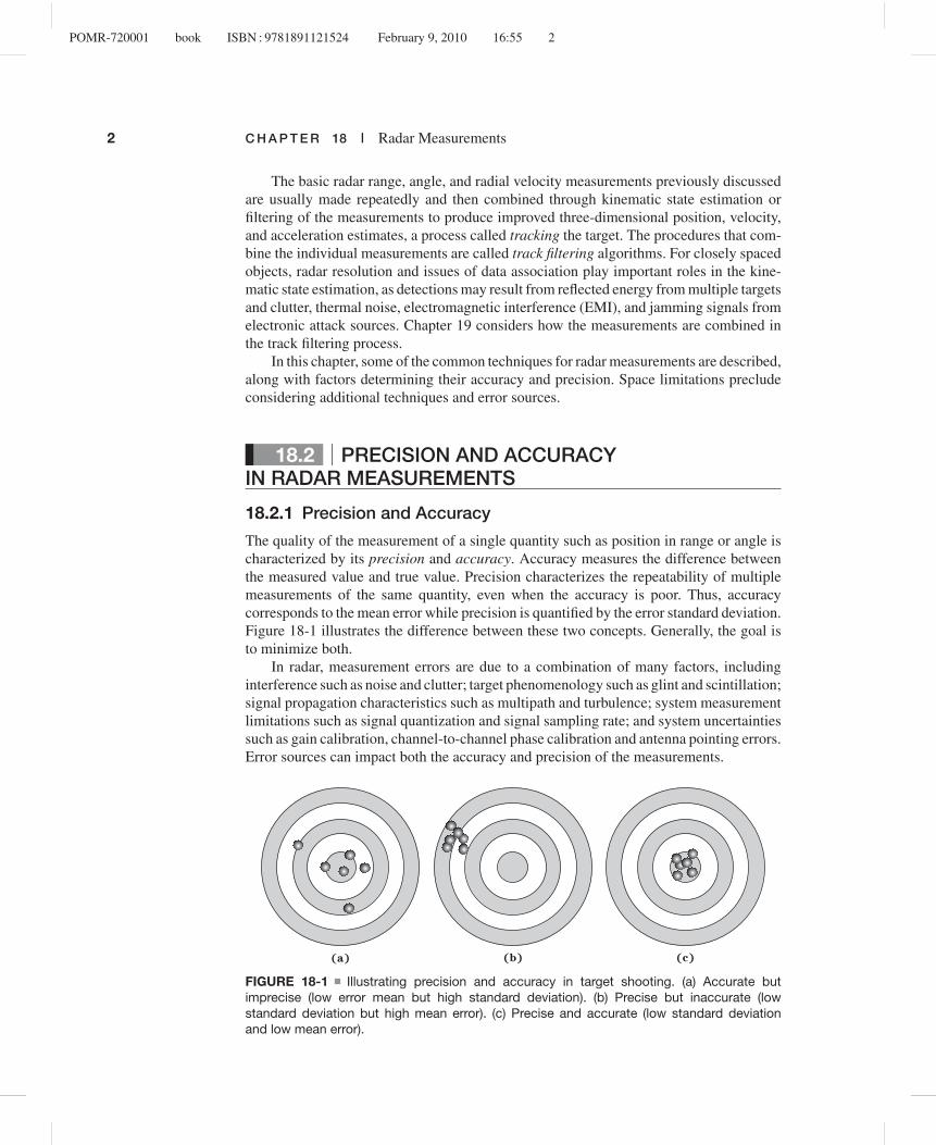
The quality of the measurement of a single quantity such as position in range or angle ischaracterized by its precision and accuracy. Accuracy measures the difference betweenthe measured value and true value. Precision characterizes the repeatability of multiplemeasurements of the same quantity, even when the accuracy is poor. Thus, accuracycorresponds to the mean error while precision is quantified by the error standard deviation.Figure 18-1 illustrates the difference between these two concepts. Generally, the goal isto minimize both.

In radar, measurement errors are due to a combination of many factors, includinginterference such as noise and clutter; target phenomenology such as glint and scintillation;signal propagation characteristics such as multipath and turbulence; system measurementlimitations such as signal quantization and signal sampling rate; and system uncertaintiessuch as gain calibration, channel-to-channel phase calibration and antenna pointing errors.Error sources can impact both the accuracy and precision of the measurements.

(a) (b) (c)

FIGURE 18-1 Illustrating precision and accuracy in target shooting. (a) Accurate butimprecise (low error mean but high standard deviation). (b) Precise but inaccurate (lowstandard deviation but high mean error). (c) Precise and accurate (low standard deviationand low mean error).


18.2 Precision and Accuracy in Radar Measurements 3

No

rmal

ized

Am

pli

tud

e

Time (multiples of t )

0

0.2

0.4

0.6

0.8

1.0

1.2

1.4

–2 –1.6 –1.2 –0.8 –0.4 0 0.4 0.8 1.2 1.6 2

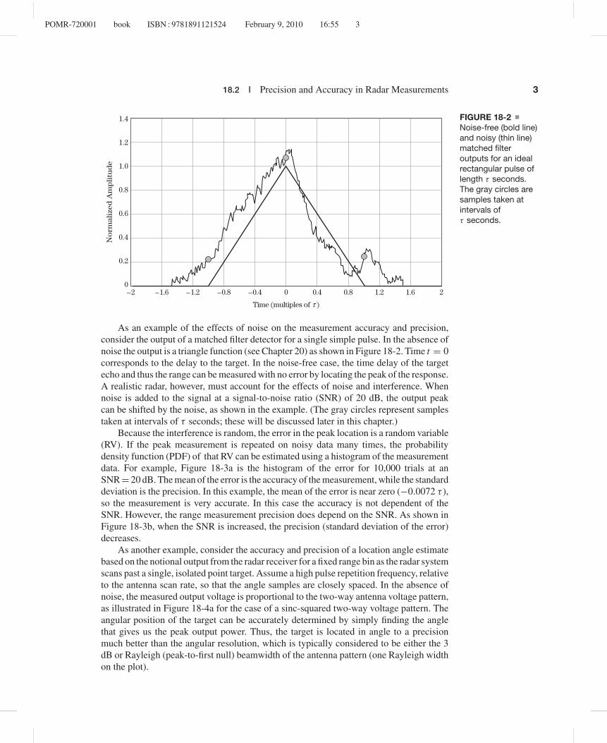
FIGURE 18-2Noise-free (bold line)and noisy (thin line)matched filteroutputs for an idealrectangular pulse oflength τ seconds.The gray circles aresamples taken atintervals ofτ seconds.

As an example of the effects of noise on the measurement accuracy and precision,consider the output of a matched filter detector for a single simple pulse. In the absence ofnoise the output is a triangle function (see Chapter 20) as shown in Figure 18-2. Time t = 0corresponds to the delay to the target. In the noise-free case, the time delay of the targetecho and thus the range can be measured with no error by locating the peak of the response.A realistic radar, however, must account for the effects of noise and interference. Whennoise is added to the signal at a signal-to-noise ratio (SNR) of 20 dB, the output peakcan be shifted by the noise, as shown in the example. (The gray circles represent samplestaken at intervals of τ seconds; these will be discussed later in this chapter.)

Because the interference is random, the error in the peak location is a random variable(RV). If the peak measurement is repeated on noisy data many times, the probabilitydensity function (PDF) of that RV can be estimated using a histogram of the measurementdata. For example, Figure 18-3a is the histogram of the error for 10,000 trials at anSNR = 20 dB. The mean of the error is the accuracy of the measurement, while the standarddeviation is the precision. In this example, the mean of the error is near zero (−0.0072 τ ),so the measurement is very accurate. In this case the accuracy is not dependent of theSNR. However, the range measurement precision does depend on the SNR. As shown inFigure 18-3b, when the SNR is increased, the precision (standard deviation of the error)decreases.

As another example, consider the accuracy and precision of a location angle estimatebased on the notional output from the radar receiver for a fixed range bin as the radar systemscans past a single, isolated point target. Assume a high pulse repetition frequency, relativeto the antenna scan rate, so that the angle samples are closely spaced. In the absence ofnoise, the measured output voltage is proportional to the two-way antenna voltage pattern,as illustrated in Figure 18-4a for the case of a sinc-squared two-way voltage pattern. Theangular position of the target can be accurately determined by simply finding the anglethat gives us the peak output power. Thus, the target is located in angle to a precisionmuch better than the angular resolution, which is typically considered to be either the 3dB or Rayleigh (peak-to-first null) beamwidth of the antenna pattern (one Rayleigh widthon the plot).



0

0.01

0.02

0.03

0.06

0.05

0.04

0.07

0.08

–1.5 –1.0 –0.5 0 1.50.5 1.0

Error in Peak Location (multiples of t)

(a)

Rel

ativ

e F

requ

ency

0

0.1

0.2

0.3

0.4

0.5

10 15 20 25 30 35 40

SNR (dB)

(b)

Stan

dard

Dev

iati

on o

f E

rror

FIGURE 18-3 Statistics of range estimation error using peak detection method.(a) Histogram of peak location measurement error for SNR = 20 dB and 10,000 trials.(b) Standard deviation of error versus SNR.

(a) (b)

Angle Relative to Boresight (Rayleigh widths)

Rel

ativ

e R

ecei

ved

Volt

age

–3 –2 –1 0 1 2 30

0.2

0.4

0.6

0.8

1.0

1.2

Angle Relative to Boresight (Rayleigh widths)

Rel

ativ

e R

ecei

ved

Pow

er

–3 –2 –1 0 1 2 30

0.2

0.4

0.6

0.8

1.0

1.2

FIGURE 18-4 Received voltage from an angle scan of a single-point target. (a) No noise.(b) 30 dB signal-to-noise ratio.

Now add noise or other interference to the problem. The receiver output now consistsof the sum of the target echo, weighted by the antenna pattern, and the noise. The noisemay cause the observed peak to occur at an angle other than the true target location, as seenin Figure 18-4b; the actual peak in this sample is at −0.033 Rayleigh widths. As might beimagined, the larger the noise, the greater the likely deviation of the measurement fromthe noise-free case.

As before, the measured location of the peak receiver output, and thus the estimatedangle to the target, is now a random variable. If the peak measurement is repeated on noisydata many times, the probability density function (PDF) of that RV can be estimated usinga histogram of the measurement data. Figure 18-5 is an example of the histogram for theobserved peak location when additive complex Gaussian noise is included for two valuesof peak signal-to-noise ratio. The difference between the mean of the PDF of the peak


18.2 Precision and Accuracy in Radar Measurements 5

(a) (b)

Angle Error (Rayleigh widths)

Pro

babi

lity

Den

sity

–0.5 –0.4 –0.3 0–0.1–0.2 0.1 0.40.30.2 0.50

1

3

2

6

5

4

7

9

8

10

Angle Error (Rayleigh widths)

Pro

babi

lity

Den

sity

–0.5 –0.4 –0.3 0–0.1–0.2 0.1 0.40.30.2 0.50

1

3

2

6

5

4

7

9

8

10

FIGURE 18-5 Histograms of angle error using peak power method. The dark curve is azero-mean Gaussian PDF with the same variance as the error data. The center dashed lineindicates the data mean, with secondary dashed lines at one standard deviation from themean. (a) 30 dB SNR at boresight. (b) 10 dB SNR at boresight. Note the wider spread(larger standard deviation) of errors at lower SNR.

location and the actual target location is the accuracy of the angle measurement, while thestandard deviation of the PDF is the precision of the measurement. In Figure 18-5b, theSNR is 20 dB lower than in 18.5a, a factor of 100. Note that the angle error distributionis wider in the lower SNR case, that is, has a higher variance. In this example, in fact,the variance of the distribution in Figure 18-5b is 9.54 times that of the distribution inFigure 18-5a. This factor is approximately the square root of the 100× change in SNR,suggesting that the variance of the angle estimation error is inversely proportional to thesquare root of the SNR. The precision is therefore inversely proportional to the fourth rootof SNR. On the other hand, the expected value of the error in the peak location is zero forboth values of SNR, and hence the accuracy is high and independent of the SNR.

Noise is not the only limitation on measurement quality. Other factors such as reso-lution and sampling density also come into play. For example, in the angle measurementcase, the output power is not measured on a continuous angle axis but only at discreteangles determined by the radar’s PRF and the antenna scan rate, resulting in quantizationof the angle estimates. Quantization also occurs due to discretized range bins (e.g., thegray circles in Figure 18-2) and arises in sampling and digital signal processing of the sig-nal. Quantization effects can degrade both accuracy and precision; however, considerationof quantization effects is outside of the scope of this chapter. Resolution and samplingdensity are considered further in Section 18.5.

18.2.2 Accuracy and Performance Considerations

The emphasis in the chapter is on measurement precision. Nevertheless, accuracy con-siderations are important. Factors affecting measurement accuracy include not only noiseand resolution but also signal and target characteristics and radar hardware considerations.For example, any uncertainty in the antenna boresight angle, due for example to mountingor pattern calibration errors or uncertainty, will affect the accuracy of a location measure-ment. Radiofrequency (RF) hardware or antenna gain calibration errors (gain uncertainty)will affect the accuracy of target signal power measurements. Mismatched in-phase (I) and



quadrature (Q) channels in the receiver can adversely affect both power and phase mea-surements [1] and may bias range measurements when range compression is used. Systemtiming and frequency error and stability also degrade accuracy. Signal propagation effectsare another important factor in overall measurement accuracy: atmospheric refraction ofthe radar signal and multipath can introduce pointing and range measurement error. All ofthese effects shift the mean of the parameter measurement, thereby degrading the accuracy.

Because a key source of accuracy degradation is due to error in the values assumedand used for the hardware parameters such as receiver gain, care must be taken to measureor calibrate the system and antenna gain and the antenna pointing angle and beamwidth,for example. The radar design usually includes mechanisms to minimize changes in theseparameters. Periodic system calibration is common. One technique is to incorporate acalibration feedback loop wherein an attenuated transmit signal is fed into the antenna orreceiver to measure the receiver power from which the system gain can then be inferred.While there is always some residual uncertainty, careful calibration can improve knowl-edge of the values used in computing signal power, timing, channel-to-channel phase andgain matching, and frequency measurements.

Since there is always residual uncertainty in calibration and knowledge of designparameters, how can the measurement accuracy be estimated? While a detailed treatmentof this topic is outside of the scope of this chapter, some comments are provided. A simple,commonly used approach is based on root sum of squares (RSS). The accuracy estimateis computed as the square root of the sum of the squared errors separately determined foreach error source. Specifically, given errors {δ1, δ2, . . . , δN}, the RSS estimate of the totalerror δ is

δ =√

δ21 + δ2

1 + . . . δ2N (18.1)

The RSS error effectively treats each error source as independent and Gaussian.To use RSS, an estimate of the uncertainty of each error source is generated, usually

by the system or subsystem designer. For example, suppose that for a particular radarthe uncertainty in azimuth boresight pointing angle of the antenna is estimated in testingto be ±0.03 degrees. This implies that the actual pointing angle is unknown but fallswithin this range. Alternately, this is the expected range of pointing angle errors formultiple antennas made for the project. Continuing the example, suppose the antennamounting error is expected to fall in the range of ±0.05 degrees. The RSS of these valuesis

√(0.03)2 + (0.05)2 = 0.058 degrees.The RSS technique provides an imperfect, but often reasonably realistic, estimate of

the expected pointing error for a particular unit. RSS estimates are popular because theydo not require the knowledge of the individual error PDFs needed for more sophisticatederror estimation based on signal flow model approaches. Worst-case analysis can also beused and results in a more conservative estimate.

Errors in antenna other estimated parameters such as signal power, the effects of eachof the pointing errors on the power are determined. Typically, this is done using nominalvalues of the radar’s operational parameters and the value of the error source is varied.The difference in the power for zero error and values within the range is computed. In thecase of antenna pointing errors, the effective antenna gain in the direction of the targetis altered. The estimated power difference is the combined effects of other error sourcesusing RSS to yield an estimate of the range of the expected power error (i.e., an error barfor the power measurement accuracy).


18.3 Radar Signal Model 7

Errors in one system parameter also result in errors in other radar measurements.Continuing the example, antenna pointing errors alter the antenna gain in the direction ofa target, in turn altering the received echo power. Typically, the effect of each source ofpointing error on the power is determined by assuming the nominal values of the radar’sother operational parameters (e.g., transmitted power, system losses) and varying onesource of pointing error to estimate the resulting variation in received power. The powervariances due to each identified error source are combined using the RSS technique toprovide an estimate of the range of the expected power error.

18.3 RADAR SIGNAL MODEL

The radar range equations presented in earlier chapters of this book are expressions ofaverage power or energy and are often used for system-level trade studies in radar systemdesign and analysis. However, radar measurements are typically formed with the voltagesignals. Thus, the voltage form of the radar signals is used for the modeling and analysisof radar measurements for tracking studies. Since voltage is proportional to the squareroot of power, a general model of the RF echo signal received in the radar, for eithera conventional antenna or the sum channel of a monopulse from a single target, can bewritten as

s(t) = 2

√Pt

(4π)3

λ

R2ξV 2

� (θ, ψ) p (t) cos (ωct + ωd t + φ) + w� (t) (18.2)

where

Pt = transmitted power.

λ = wavelength.

R = range to target.

ξ = voltage reflectivity of the target.

G�(θ, ψ) = voltage gain of the antenna at the angles (θ, ψ) .

(θ, ψ) = angular location of the target relative to antenna boresight.

p(t) = envelope of the matched filter output for the transmitted pulse.

ωc = carrier frequency of the transmitted waveform.

ωd = Doppler shift of the received waveform.

φ = phase of the target echo.

w�(t) = receiver noise.

The “voltage reflectivity,” ξ , of the target is related to its RCS σ according to

σ = ξ 2/2 (18.3)

Note that in equation (18.2) the normalized antenna voltage gain pattern V�(θ, ψ) isassumed to be the same on transmit and receive, so the two-way pattern is V 2

�(θ, ψ) asshown. The antenna gain pattern is assumed to be the product of two orthogonal voltagepatterns,

V�(θ, ψ) = W (θ)U (ψ) (18.4)

where W (θ) and U (ψ) are the elevation and azimuth voltage patterns, respectively.



Demodulation by coherent mixing with quadrature oscillators at the frequency ωc

removes the carrier term of equation (18.2), as described in Chapter 11. Two commonsources of error frequently reduce the measured amplitude of the signal s(t). First, if s(t)is mixed with ωc rather than ωc + ωd , a frequency mismatch occurs in the matched filterfor p(t), resulting in a loss in SNR referred to as Doppler loss, as discussed in [2,4] andin Chapter 20. When attempting to use a radar system designed for air targets to detectand track space targets traveling at significantly higher velocity, the Doppler loss can besufficiently high to prevent detection. Second, the need to detect targets at a priori unknownranges and to detect multiple, closely spaced objects in the same dwell dictates that theoutput of the matched filter be sampled periodically in fast time at the bandwidth of thesignal over the range interval (range window) of interest. There is no guarantee that one ofthe samples will fall on the peak of the matched filter response, as seen in the example inFigure 18-2. Instead, the energy of a target echo may be captured in adjacent samples thatstraddle the peak, reducing the measured SNR. This reduction in SNR is often referred toas straddle loss. However, as will be seen, the signals in the adjacent cells can be used toimprove the range estimate precision beyond the resolution and to reduce straddle loss.

Ignoring any Doppler and straddle losses, the I and Q components of the sampledoutput of the matched filter with gain p0 are given by

sI = α cos φ + w� I sQ = α sin φ + w�Q (18.5)

where

α =√

Pt

(4π)3/2λ

R2ξV 2

�(θ, ψ)p0, w� I ∼ N(0, σ 2

�

/2), w�Q ∼ N

(0, σ 2

�

/2)

(18.6)

where

p0 = pulse amplitude.

σ 2� = kT0 Fn BIF = total noise power at the receiver output.

k = Boltzmann’s constant.

T0 = 290 ◦K = standard noise temperature.

Fn = receiver noise figure.

BIF = receiver intermediate frequency bandwidth.

The other variables are as given previously, and the notation∼N(0, σ 2) indicates a normallydistributed (Gaussian) random variable with zero mean and a variance of σ 2. Any gaindue to coherent integration such as pulse compression, moving target indication (MTI),or pulse-Doppler processing with a discrete Fourier transform (DFT) is included in sI

and sQ . The integration of sI and sQ from multiple pulses after pulse compression andDoppler processing is typically accomplished using only the measured amplitude of thepulses, ignoring the phase, and is referred to as noncoherent integration. Often, channel-dependent calibration corrections for gain, time delay, and phase shift are also applied tothe measured values to improve their accuracy.

Letting � and ϕ denote the measured amplitude and phase of the signals in equa-tion (18.5), including the calibration corrections and noise contributions, gives

sI = � cos ϕ, sQ = � sin ϕ (18.7)


18.4 Parameter Estimation 9

It is useful to define the observed SNR as the ratio of total signal power to total noise power

SNRobs = �2

σ 2�

(18.8)

� includes both signal and noise contributions, so SNRobs is actually a signal-plus-noise-to-noise ratio. The SNR of a target can therefore be computed for the expected value ofthe observed SNR, that is,

SNR = E{SNRobs} − 1 (18.9)

where E{·) denotes the expected value.

18.4 PARAMETER ESTIMATION

The goal of the radar measurement process is to estimate the various parameters of thetarget reflected in the signal s(t). The primary parameters of interest include the reflectivityamplitude, ξ , the Doppler shift, ωd , the angular direction to the target, (θ, ψ), and the timedelay to the target, which is reflected in the sampling time at which the signal was measuredand in the signal phase, φ. Before addressing techniques for measuring each of these, it isuseful to first discuss the general idea of an estimator and the achievable precision.

18.4.1 Estimators

Consider an observed signal y(t) that is the sum of a target component s(t) and a noisecomponent w(t):

y(t) = s(t) + w(t) (18.10)

The signal y(t) is a function of one or more parameters θi . These might be, for example, thetime delay, amplitude, Doppler shift, or angle of arrival (AOA) of the target component.The goal is to estimate the parameter values given a set of observations of y(t). This isdone using an estimator.

Suppose y(t) is sampled multiple times (intrapulse or over multiple pulses) to producea vector of N observations,

y = {y1, y2, . . . yN } (18.11)

Because of the noise, the data y is a random vector that depends on the parameter θ .Thus, y is described by a conditional PDF p(y|θ ). Now define an estimator f of a parameterθ based on the data y,

θ = f (y) (18.12)

Because y is random, the estimate θ is also a random variable and therefore has a probabilitydensity function with a mean and variance.

Two desirable properties of an estimator are that it be unbiased and consistent. Thesemean that the expected value of the estimate equals the actual value of the parameter,and that the variance of the estimate decreases to zero as more measurements becomeavailable:

E{θ} = θi (unbiased)

limN→∞

{σ 2

θ

} → 0 (consistent)(18.13)



In other words, a desirable estimator produces estimates that are, on average, accurate andwhose precision improves with more data.

A simple example of a good estimator is one that estimates the value of a constant signalA in the presence of white (and thus zero-mean) noise w[n] of variance σ 2

w by averaging Nsamples of the noisy signal y[n] = A +w[n]. In this case, the parameter θ is the unknownamplitude A, the vector y is composed of the N samples of y[n], and the estimator is

A = f (y) = 1

N

N−1∑n=0

y[n]

= 1

N

N−1∑n=0

(A + w[n]) = A + 1

N

N−1∑n=0

w[n] (18.14)

Note that the expected value of A = A, so the estimator is unbiased. The variance of thesecond (noise) term is σ 2

w

/N ; this is also the variance of A. Thus, the variance of the es-

timator tends to zero as the number of data samples increases, so it is also consistent. Theexpected value of the square root of the variance (the standard deviation) of the estimateis the measurement precision.

The absolute value of the variance of the estimate is less significant than its valuerelative to the value of A. Normalizing the estimator variance by the signal power A2 givesthe normalized measurement variance

σ 2w

NA2 = 1

N · SNR(18.15)

where the SNR for this problem is A2/σ 2

w . The normalized estimate variance is thus anexample of an estimator whose variance is inversely proportional to the SNR.

Many types of estimators exist. Two of the most commonly used are minimum vari-ance (MV) estimators and maximum likelihood (ML) estimators. A minimum variance orminimum variance unbiased (MVU) estimator is one that is both unbiased and minimizesthe mean square error between the actual value of the parameter being estimated and itsestimate [3]. In the context of this chapter, it minimizes (θ − θ)2 under the condition thatE{θ} = 0.

The maximum likelihood estimator is one that chooses θ to maximize the likelihoodof the specific observed data values y. For example, suppose an observed signal sample, s,is assumed to be the sum of a constant value, A, and zero-mean Gaussian noise of variance,σ 2. The observation s is then Gaussian with mean A and variance σ 2, s ∼ N(A, σ 2). Thegoal is to estimate the mean. For concreteness, suppose A = 3 and σ 2 = 1, and a singlemeasurement results in the observed value s = 2.8. The ML estimate of A based on sis AML = 2.8 because that is the value of the Gaussian mean that maximizes the chancethat the measured value is 2.8. As will be seen later, if multiple measurements of s areavailable, the ML estimator of A is the sample mean.

The ML estimator is often a good practical choice because its form is often relativelyeasy to determine. In addition, in the case of Gaussian noise it is equivalent to the MVestimator and thus is the optimum estimator.

As previously noted the standard deviation of the estimate error describes the measure-ment precision. The standard deviation depends on the estimator chosen, and sometimescan be hard to compute for a particular estimator. However, as described in the followingsection, the error standard deviation can be bounded.



18.4.2 The Cramer-Rao Lower Bound

In the angle measurement example in Section 18.2.1, it was seen that the variance of theangle estimate decreased with increasing SNR. Similar behavior is typically observed forrange and Doppler estimates as well. Specifically, for a parameter θ , the variance σ 2

θof

the estimated value θ often behaves as

σ 2θ

= k

SNR(18.16)

for some constant k. Is this behavior predictable and, if so, what can be said about theconstant k?

The Cramer-Rao lower bound (CRLB) is a famous result that addresses these ques-tions. The CRLB, J(θ ), establishes the minimum achievable variance (square of precision)of an unbiased estimator of the parameter θ . The square root of the CRLB is thus the bestachievable precision. Any particular unbiased estimator must have a variance equal to orgreater than the CRLB, and the quality of a particular estimator can be judged by howclose its actual variance comes to achieving the CRLB.

An important metric for describing an estimator’s performance is the root mean square(RMS) error. For zero-mean error the square root of the CRLB is the minimum achiev-able RMS error. While the CRLB does not depend on the estimator, the RMS error is afunction of the estimator employed.

Derivation of the CRLB is beyond the scope of this chapter; good (and very similar)derivations are given in [3,4]. The bound states that the minimum variance in the estimateθ is

σ 2θ

≥ J (θ) = 1

E[{∂ ln {p(y|θ)}/∂θ}2] (18.17)

where p(y|θ) is the conditional probability density function (PDF) of the data vector ygiven some particular value of the parameter θ . Under some mild conditions, the CRLBhas an alternate form,

σ 2θ

≥ J (θ) = −1

E[∂2 ln {p (y|θ )}/∂θ2

] (18.18)

The choice between equation (18.17) or (18.18) is a matter of convenience, depending onthe functional form of ln{p(y|θ )}. More general forms of the CRLB that include bias arepossible [3,4].

The CRLB can be further simplified for the special but very common and importantcase of a signal in additive Gaussian noise. Suppose the data y is N observations of a realdiscrete signal s that is a function of some parameter θ in real white Gaussian noise,

y[n] = s[n; θ ] + w[n], n = 0, . . . , N − 1, w[n] ∼ N(0, σ 2

w

)(18.19)

Starting from equation (18.18), it can be shown that for this case the CRLB is [3]

J (θ) = σ 2w

N−1∑n=0

(∂s[n; θ ]

∂θ

)2 (18.20)



It is sometimes more convenient to deal with continuous time rather than sampledsignals. The continuous time equivalents to equations (18.19) and (18.20) are

y(t) = s(t ; θ) + w(t), −T/

2 ≤ t ≤ T/

2, w(t) ∼ N(0, σ 2

w

)(18.21)

J (θ) = σ 2w

T/2∫t=−T/2

(∂s(t ; θ)

∂θ

)2

dt

(18.22)

where T is the duration of the signal of interest.As a simple illustration of equation (18.20), consider estimating the value of a constant

m in Gaussian noise. In this case, s[n; θ ] = m, so ∂s[n; θ ]/∂θ = ∂(m)

/∂m = 1 and the

CRLB for estimating m becomes

J (θ) = J (m) = σ 2w

N, (18.23)

which is achieved for the mean estimator in equation 18.14 and shows that, as expected, theminimum achievable variance of the estimate decreases with the number of measurementsavailable. A better metric than the variance in m is the variance normalized to the actualsignal power m2, i.e. the relative error. The CRLB for this quantity is

J(

m

m

)= σ 2

w

N · m2= 1

N · SNR(18.24)

Notice that the CRLB of the normalized error estimate varies as 1/SNR. This proves to bethe case in many radar parameter estimation problems.

18.4.3 Precision and Resolution for the Gaussian Case

Equation (18.20) states that the minimum achievable precision of a measurement increasesas the square of the derivative of the signal with respect to the parameter of interestincreases. Loosely interpreted, the more rapidly the signal varies, the better the precision.For example, if the parameter of interest is range, then a matched filter output with asteep leading and trailing edge will allow better range measurement precision than abroad, slowly rising and falling output waveform. Similarly, a narrow antenna mainlobeshould allow better angular precision than a wide one. This should not seem surprising.A waveform with sharp edges suggests a high bandwidth in the dimension of interest:temporal bandwidth in time or range or spatial bandwidth in angle. Thus, it might beanticipated that higher bandwidths lead to lower CRLBs, at least in the Gaussian noise case.

This is in fact the case. As an example, consider time-delay estimation. The parameterθ in equation (18.20) is then the time delay, t0, of the signal echo, and the signal itself is

s[n; θ ] = s[nTs − t0] (18.25)

where Ts is the sampling interval in fast time. Using equation (18.25) in (18.20), severalreferences [3–5] derive the result that

σ 2t0 ≥ J (t0) = 2E

N0· 1

B2rms

(18.26)



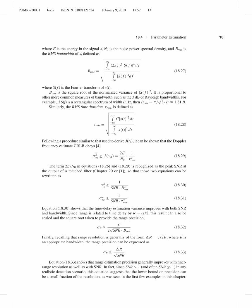
where E is the energy in the signal s, N0 is the noise power spectral density, and Brms isthe RMS bandwidth of s, defined as

Brms =

√√√√√√√√∞∫

−∞(2π f )2|S( f )|2 d f

∞∫−∞

|S( f )|2d f(18.27)

where S( f ) is the Fourier transform of s(t).Brms is the square root of the normalized variance of |S( f )|2. It is proportional to

other more common measures of bandwidth, such as the 3 dB or Rayleigh bandwidths. Forexample, if S(f) is a rectangular spectrum of width B Hz, then Brms = π/

√3 · B ≈ 1.81 B.

Similarly, the RMS time duration, τrms, is defined as

τrms =

√√√√√√√√∞∫

−∞t2|s(t)|2 dt

∞∫−∞

|s(t)|2 dt(18.28)

Following a procedure similar to that used to derive J(t0), it can be shown that the Dopplerfrequency estimate CRLB obeys [4]

σ 2ωd

≥ J (ωd) = 2E

N0· 1

τ 2rms

(18.29)

The term 2E/N0 in equations (18.26) and (18.29) is recognized as the peak SNR atthe output of a matched filter (Chapter 20 or [1]), so that those two equations can berewritten as

σ 2t0 ≥ 1

SNR · B2rms

(18.30)

σ 2ωd

≥ 1

SNR · τ 2rms

(18.31)

Equation (18.30) shows that the time-delay estimation variance improves with both SNRand bandwidth. Since range is related to time delay by R = ct/2, this result can also bescaled and the square root taken to provide the range precision,

σR ≥ c

2√

SNR · Brms(18.32)

Finally, recalling that range resolution is generally of the form �R = c/2B, where B isan appropriate bandwidth, the range precision can be expressed as

σR ≥ �R√SNR

(18.33)

Equation (18.33) shows that range estimation precision generally improves with finer-range resolution as well as with SNR. In fact, since SNR > 1 (and often SNR � 1) in anyrealistic detection scenario, this equation suggests that the lower bound on precision canbe a small fraction of the resolution, as was seen in the first few examples in this chapter.



For instance, if SNR = 10 (10 dB), the lower bound on precision above is 32% of the RMSrange resolution; if it is 100 (20 dB), the bound is 10% of the RMS resolution. In manypractical systems, however, system limitations and signal variability create additionallimits on estimation precision.

18.4.4 Signal and Target Variability

The derivations presented in the previous sections are based on the assumption that thetarget and signal characteristics remain stationary over the time period required to collectthe samples. If the target characteristics or the signal propagation conditions vary overthe sampling period, signal variability is introduced, which increases the estimate varia-tion and thus degrades the measurement precision. A major source of target variability ischanges in the target aspect angle that cause scintillation (exponentially distributed fluc-tuations of the target RCS as described in Chapter 15) and glint. Glint is a fluctuation ofthe apparent angle of the target relative to the radar boresight caused by variations in theorientation of the phase front of the echo signal at the antenna, possibly due to changes inthe scattering location on the target. Multipath and diffraction in the signal path can alsointroduce signal fluctuation as well as possible multiple apparent targets.

If appropriate models for signal and target variability are available, these can beincluded in the probability density function used in deriving measurement estimators andcomputing the CRLB. In the interest of clarity and brevity, only a few specific Swerlingcases for signal and target variability are considered in this chapter.

18.5 RANGE MEASUREMENTS

The previous discussion considered range measurement precision. Additional methodsand accuracy analyses are provided in this section after a discussion on the effects ofresolution and sampling. Note that although the discussion on resolution and samplingfocuses on range and angle measurement, these issues also impact phase and Dopplermeasurement.

18.5.1 Resolution and Sampling

A typical radar collects target returns for each transmitted pulse over some finite time-delay interval or range window. The start of the range window may be positioned at anyrange beyond the blind range of the radar. The output of the matched filter is sampledperiodically over the range window, usually at a spacing equal to the bandwidth of thewaveform but sometimes at higher rates, for example, in a dedicated tracking mode. Thus,the time delay or range estimation is accomplished with a sequence of periodic samplesof the matched filter output.

The range resolution of the radar can be generally expressed as (see Chapter 20)

�R = αc

2B(18.34)

where B is the waveform bandwidth, and α is a factor in the range 1 < α < 2 that representsthe degradation in range resolution resulting from system errors or range sidelobe reductiontechniques such as windowing. The bandwidth, B/α, corresponds to the bandwidth of the


18.5 Range Measurements 15

intermediate frequency (IF) filter and defines the Nyquist sampling rate at the output ofthe matched filter unless some technique such as stretch processing as discussed in [1] isemployed.

Most radars sample the receiver output at a rate of approximately 1 to 1.5 samplesper 3 dB resolution cell in range and angle. For a simple pulse waveform, B ≈ 1/τ

so that the matched filter output of Figure 18-2 would be sampled approximately everyτ seconds. Figure 18-2 illustrated this sampling strategy. Depending on the alignmentof the target’s actual range with the sampling times, only two to three samples may betaken on the response to a single-point target. This sparse set of measurements must beused to estimate the peak location. The coarsely time-quantized nature of the samplingcontributes to variability in the resulting estimates. In contrast, radars designed primarilyfor precision tracking may provide many more samples per resolution cell, allowing theuse of different techniques.

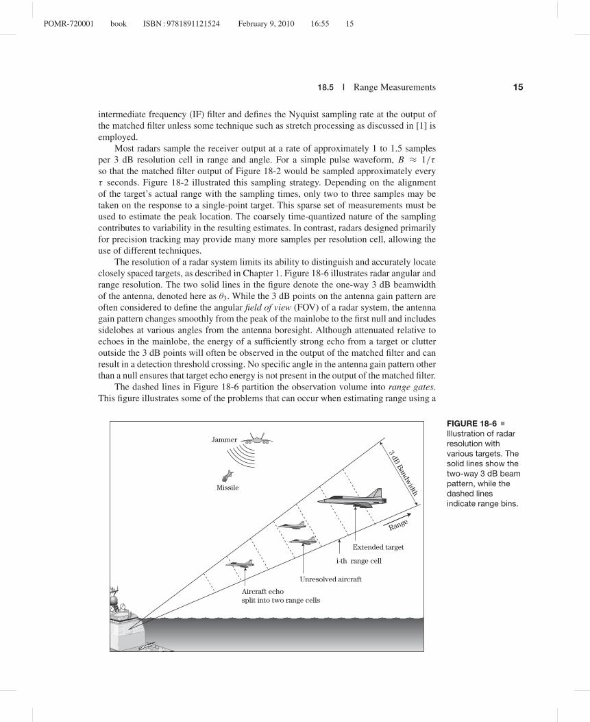
The resolution of a radar system limits its ability to distinguish and accurately locateclosely spaced targets, as described in Chapter 1. Figure 18-6 illustrates radar angular andrange resolution. The two solid lines in the figure denote the one-way 3 dB beamwidthof the antenna, denoted here as θ3. While the 3 dB points on the antenna gain pattern areoften considered to define the angular field of view (FOV) of a radar system, the antennagain pattern changes smoothly from the peak of the mainlobe to the first null and includessidelobes at various angles from the antenna boresight. Although attenuated relative toechoes in the mainlobe, the energy of a sufficiently strong echo from a target or clutteroutside the 3 dB points will often be observed in the output of the matched filter and canresult in a detection threshold crossing. No specific angle in the antenna gain pattern otherthan a null ensures that target echo energy is not present in the output of the matched filter.

The dashed lines in Figure 18-6 partition the observation volume into range gates.This figure illustrates some of the problems that can occur when estimating range using a

Extended target

Range

i-th range cell

Unresolved aircraft

Aircraft echosplit into two range cells

3 dB B

andwidthMissile

Jammer

FIGURE 18-6Illustration of radarresolution withvarious targets. Thesolid lines show thetwo-way 3 dB beampattern, while thedashed linesindicate range bins.



sampling interval equal to the range resolution. Each range cell is associated with a sampleof the output of the matched filter through which the received echo signal is passed. Thecenter of each range cell corresponds to the sample time. A range and angle measurementis made whenever the output of the matched filter exceeds the detection threshold. Thesmall single aircraft is smaller than the extent of the range cell, but its position straddles tworange cells, causing the echoed energy from the aircraft to be split between two adjacentrange cells and incurring a straddle loss. Typically, every measurement experiences somestraddle loss. The two closely spaced aircraft are in the same range cell, and only onemeasurement with energy from for both targets results. The large airliner extends overthree range cells. Such targets are often referred to as extended targets. Significant echoesfrom the airliner are observed in three consecutive samples of the matched filter. Part ofthe challenge in radar tracking and data association is deciding whether a sequence ofdetections is one extended target or multiple closely spaced targets. Also, the signals fromthe jammer enter into the measurements of the missile between it and the radar and affectall of the range cells that are collected along the line of sight to the missile.

Continuing the discussion on range measurement, the various situations that canresult are depicted in Figure 18-7, where the sequence of rectangles represent consecutivesamples of the matched filter output and the fraction of the target energy captured inthe sample is represented by the percentage fill of the rectangle. Some of these situationsare analogous to those depicted in Figure 18-6. On the left side of the top sequence inFigure 18-7, the reflected energy is captured in a single sample of the matched filter output.However, this is typically not the case.

FIGURE 18-7Resolving closelyspaced objects inrange.

Range or Time Delay

Range or Time Delay

Bs Δ= Signal Bandwidth

C Δ= Speed of Light

Echoed pulse from point targetwith sampling time matched

to arrival time

Rangeresolution

Two unresolved targetsOne extended target or two point

targets or three point targets?

One extended target or two pointtargets or three point targets?

Multiple targets orsingle extended target?

Echoed pulse from pointtarget with energy spread

over two samples


18.5 Range Measurements 17

The more common case is illustrated by the sample of the echo in the top rightof Figure 18-7, where the reflected energy is captured in two consecutive samples. Inthis case, the Cramer-Rao lower bound on the variance of the range estimate is closelyachieved by a power-weighted centroid of the ranges of the two consecutive samples. Thistechnique, along with the split-gate centroid method of measuring range, are describedand their precision analyzed in the next section. Examples of closely spaced single targetsand multiple targets are shown in the other rows.

Sidelobes in range, angle, or Doppler complicate measurements further. Sidelobes arealways present in angle due to the antenna sidelobes and in Doppler if the spectrum iscomputed using Fourier techniques, as will usually be the case. They will be present inrange when pulse compression techniques are used. Sidelobes result in energy from theecho of a target being present in the data samples adjacent to those that correspond to theactual target location. For example, the echo of a small aircraft target with a relatively lowRCS that is within a few of range cells of an airliner with a large RCS may be obscured bythe range sidelobes from the airliner, a phenomenon known as masking (see Chapter 17for an example of masking in the Doppler dimension). Waveform design methods andsignal windowing techniques are often employed to reduce the impacts of range sidelobes.While special signal processing techniques can be employed to assist in the detection ofunresolved or extended targets, multiple targets can appear as a single target measurementand one target can produce multiple measurements. Thus, close coordination of the signalprocessing and target tracking is needed.

18.5.2 Split-Gate and Centroid Range Measurement

In Sections 18.2.1 and 18.4.3 it was shown that target range measurement precision usingthe signal peak is dependent on the SNR. Rather than use the signal peak to estimate therange, a better approach is to use one of a number of techniques that combine multiplesamples to provide some integration against noise. One such technique is an early/late gateor split-gate tracker. This technique is suitable for signals that produce outputs symmetricabout the true location in the absence of noise. This is the case for both the angle andrange measurement examples considered so far. The early/late gate tracker slides a two-part window across the data and integrates the energy within each of the two “gates”(halves of the window). When the energy in each gate is equal, the gate is approximatelycentered on the peak signal.

One way to implement the early/late gate tracker is to convolve the noisy output withthe impulse response h[l] shown in Figure 18-8b as the solid black line overlaid on thenoisy data. The ideal (noise-free) matched filter output is shown in Figure 18-8a [see alsoFigure 18-2.] Because of the difference in sign of the impulse response in the two gates,the early/late gate tracker produces an output near zero when centered on the signal peak.This is depicted in Figure 18-9, which shows the magnitude of the output of the early/lategate tracker for input SNRs of 20 dB and 5 dB. The peak output of the matched filter(not shown) occurs at samples 99 and 107 in these two examples, while the early/lategate tracker correctly estimates the target range to be at sample 100 for the 20 dB caseand misses by only 1 sample, at range bin 101, in the noisier 5 dB case. An alternativeimplementation does not take the magnitude at the tracker output; in this case, the rangeestimate is the zero crossing in the tracker output (see Chapter 19).

The precision of an early/late gate tracker is limited to the sampling density of thesignal to which it is applied. This may be quite adequate if the data are highly oversampled



(a)

Range SampleR0 – t R0 + tR0

Am

plit

ude

0 20 40 1008060 120 180160140 200–0.2

0

0.2

0.4

0.6

1.0

0.8

1.2

(b)

Range SampleR0 – t R0 + tR0

Am

plit

ude

0 20 40 1008060 120 180160140 200–0.2

0

0.2

0.4

0.6

1.0

0.8

1.2

Early Gate Late Gate

FIGURE 18-8 (a) Triangular output of matched filter for an ideal rectangular pulse with nonoise. (b) Output with 10 dB SNR. Also shown is an early/late gate tracker impulse response.

(a)

Range Sample

Am

plit

ude

–50 0 50 100 150 200 2500

5

10

15

20

30

25

35

(b)

Range Sample

Am

plit

ude

–50 0 50 100 150 200 2500

5

10

15

20

30

25

35

FIGURE 18-9 (a) Magnitude of early/late gate tracker for simple pulse matched filteroutput with 20 dB peak SNR. (b) Output with 5 dB peak SNR.

(many samples per resolution cell), but, as discussed earlier, range is often estimated usingdata sampled at intervals approximately equal to a resolution cell. An alternative to theearly/late gate tracker is the centroid tracker. The centroid, Cx , over a region l ∈ [L1, L2]of a sequence x[l] is defined as

Cx =

L2∑l=L1

l · x[l]

L2∑l=L1

x[l](18.35)

Note that the centroid can take on a noninteger value, so it inherently interpolates betweensamples.


18.6 Phase Measurement 19

5 10 15 20 25 30 35 40 450

0.01

0.02

0.03

0.04

0.05

0.06

0.07

SNR (db)

ì SNR−1Va

rian

ce

FIGURE 18-10Example of varianceof power-weightedcentroid rangeestimation for idealsimple pulse andmatched filter. Thevariance isnormalized to therange resolution.

To demonstrate the performance of the two-point power centroid, consider an idealrectangular pulse of duration τ and a matched filter. The output of the matched filter is atriangular pulse of duration 2τ (Chapter 20; see also Figure 18-2). A square law detectoris assumed. The magnitude squared of the filter output is sampled at the nominal rangeresolution (i.e., every τ seconds). A two-point power centroid is applied and the rangeestimation error is calculated after removing the bias of the estimator for the noise-freecase. The error depends on the location of the actual target peak relative to the samplingtimes, so it is averaged over sampling times that vary by ±τ/2 seconds relative to the peak.The resulting variance of the average estimation error, normalized to the range resolution,is shown in Figure 18-10 as a function of SNR. The error variance decreases approximatelyas 1/SNR for the range of SNR shown.

An approximation to the CRLB of the range measurement for a simple, uncoded,rectangular pulse is given in [6] as

σ 2R ≥ c2τ

8SNR · BIF(18.36)

where BIF is the bandwidth of the IF filter, and τ is the pulse duration. A power-weightedcentroid of the ranges of the two consecutive samples approaches this CRLB. More detailon measurement precision for closely spaced targets is given in [6]. Resolving two closelyspaced targets in range is addressed in [7,8]. When range is measured with a linear fre-quency modulated (LFM) waveform, any uncompensated Doppler shift results in a shift inthe apparent range of the target, a phenomenon called range-Doppler coupling (see Chap-ter 20). The CRLB for range measurement using an LFM waveform with a rectangularenvelope and a known range rate is given in [9] as

σ 2R ≥ J (R) = 3c2

8π2SNR · B2(18.37)

where B is the swept bandwidth of the LFM waveform.

18.6 PHASE MEASUREMENT

Estimating the echo time of arrival using the methods previously described ignores thesignal phase. However, signal phase can also be estimated if the Doppler shift is known.Combining terms to simplify the signal model in equation (18.1) when the frequency is



known, the radar return can be written as

s(t) = p(t) cos(ωt + ϕ) (18.38)

where ω is the frequency, and ϕ is the carrier phase. It can then be shown that the optimalestimator for the phase is [4]

ϕ = − tan−1 Ps

Pc(18.39)

Ps =∫

p(t) sin(ωt)dt Pc =∫

p(t) cos(ωt)dt

where the sine and cosine filter integrals are over the analysis time window. When theSNR is sufficiently large the RMS error is [4]

σ 2ϕ ≥ 1

SNR · τ B(18.40)

where τ B is the pulse time-bandwidth product. Note that, like range estimation, the phasemeasurement variance is inversely proportional to the measurement SNR.

18.7 DOPPLER AND RANGE RATEMEASUREMENTS

In most modern tracking radars, range rate measurements are accomplished by pulsedDoppler waveforms that include a periodic sequence of pulses. In pulse-Doppler process-ing, the output of the matched filter is sampled throughout the range window for each pulsefor time-delay (i.e., range) estimation, and samples of the matched-filter output from themultiple pulses at each range are processed with a DFT to estimate the Doppler frequency,fd (also known as range rate, R). The Doppler resolution is the inverse of the duration ofthe pulse-Doppler waveform dwell time, Td (see Chapter 14),

� fd = 1

Td(18.41)

Because velocity is related to Doppler shift according to fd = 2v/λ, the resolution ofvelocity or range rate is

�v = �R = c

2Td ft= λ

2Td(18.42)

where ft is the carrier frequency of the transmitted waveform.Pulse-Doppler waveforms suffer potential ambiguities in range and range rate. The

minimum unambiguous range is

Rua = c

2PRI (18.43)

For a slow-time sampling interval (PRI) of T seconds, the ambiguous interval in Dopplerfrequency is 1/T Hz. Assuming both positive and negative frequencies (and thus rangerates) are of interest, the maximum unambiguous Doppler frequency, velocity, and range


18.7 Doppler and Range Rate Measurements 21

rate are then given by

fdua = ± 1

2PRI= ±PRF

2

vua = Rua = ±λ

2PRF = ± c

2 ftPRF

(18.44)

Thus, the range rate resolution is specified by the dwell time of the waveform, while themaximum unambiguous range rate is specified by the PRF of the waveform.

The CRLB for measuring frequency in hertz for the signal model of equation (18.2)with M measurements, assuming the initial phase and amplitude are also unknown, isshown by several authors to be [3,4]

σ 2f ≥ J ( f ) = 3 f 2

s

π2SNR · M(M2 − 1)≈ 3 f 2

s

π2SNR · M3Hz2 (18.45)

where fs is the sampling frequency in samples/second. Notice that the CRLB decreases asM3. One factor of M comes from the increase in SNR when integrating multiple pulses,while a factor of M2 comes from the improved resolution of the frequency estimate. Thiscan be seen by putting equation (18.45) into terms of resolution and SNR for the case ofan estimator based on the discrete-time Fourier transform (DTFT), of which the DFT isa special case. The Rayleigh frequency resolution in hertz of an M-point DFT is fs/M,and the SNR of a sinusoidal signal in the frequency domain is M times the time-domainSNR, assuming white noise (see Chapter 14). Denoting the frequency domain resolutionand SNR as � f and SNR f , equation (18.45) becomes

σ f ≥√

3

π

� f√SNR f

Hz (18.46)

Equation (18.46) states that the precision of the frequency estimate is proportional tothe resolution divided by the square root of the applicable SNR, analogous to the rangeestimation case of equation (18.33).

A number of single and multi-pulse frequency estimation schemes exist. These canbe divided into coherent and noncoherent techniques [4]. Several are considered in thefollowing. Other general frequency estimation techniques are considered in [3].

18.7.1 DFT Methods

An obvious estimator of Doppler frequency is the discrete Fourier transform, usuallyimplemented with the fast Fourier transform (FFT) algorithm. Given M samples of slowtime data y[m], the K-point DFT is

Y [k] =M−1∑m=0

y[m] exp[− j2πmk

/K

], k = 0, . . . , K − 1 (18.47)

where K ≥ M . The DFT and its properties are discussed extensively in Chapter 14.The frequency of a signal is estimated by computing its DFT and then finding the

value of k that gives the largest value of Y[k], that is, by finding the peak of the DFT. Thek-th index corresponds to a frequency of k·PRF/K Hz. Consider a signal

y[m] = A exp [ j2π f0mT ] + w[m], m = 0, . . . , M − 1 (18.48)



where w[m] is white Gaussian noise with power σ 2w . The SNR of the individual data

samples is A2/σ 2

w . The DFT effectively integrates the M data samples, increasing the SNRto a maximum of MA2

/σ 2

w if f0 equals one of the DFT frequencies. If f0 does not equalone of these frequencies, the integrated SNR is up to 3.92 dB lower (depending on thefrequency difference and the data window used; see Chapter 14 for details). This reductionis another example of straddle loss.

If the integrated SNR is at least 10 dB, it is virtually certain that the DFT peak willoccur at the index closest to the true frequency as desired. Then, for a sinusoidal signal atan arbitrary frequency f0, the maximum error in the estimated frequency f 0 is PRF/2K Hz.Thus, increasing the DFT size reduces the maximum frequency estimation error, at thecost of increased computational load for the larger DFT. The same CRLB for frequencyestimation given by equation (18.45) applies [3].

18.7.2 DFT Interpolation Methods

Frequency estimation precision can be improved following the DFT calculation with one ofa number of interpolation methods. The centroiding technique discussed earlier for rangeprocessing can be applied to the DFT also. Another common method is to fit a low-orderpolynomial through the DFT peak and its nearest neighbors. The estimated frequency isthe location of the peak of the interpolated polynomial. A typical interpolator, using onlythe magnitude of the DFT samples, estimates the frequency as [10]

�k = − 12 {|Y [k0 + 1]| − |Y [k0 − 1]|}

|Y [k0 − 1]| − 2|Y [k0]| + |Y [k0 + 1]|f 0 = (k0 + �k)

KPRF

(18.49)

where k0 is the index at which the DFT peak occurs. Figure 18-11a shows the precision ofthis estimate, f0 − f 0, as a function of the starting offset f0 − k0PRF

/K for M = 30 data

samples and various DFT sizes K. Note that the precision improves as the DFT sizeincreases.

0 0.05 0.1 0.15 0.2 0.25 0.3 0.35 0.4 0.45 0.50.0001

0.001

0.01

0.1

1

Offset (bins)

Off

set

Err

or M

agni

tude

(bi

ns) K = 30

38

45

6090

0 0.05 0.1 0.15 0.2 0.25 0.3 0.35 0.4 0.45 0.50.0001

0.001

0.01

0.1

1

Offset (bins)

Off

set

Err

or M

agni

tude

(bi

ns)

456038

90

K = 30

(a) (b)

FIGURE 18-11 Precision of DFT interpolators. Data length M = 30. (a) Magnitude only.(b) Magnitude and phase.


18.7 Doppler and Range Rate Measurements 23

Figure 18-11b shows the precision of a similar interpolator that uses the complex DFTdata instead of just the magnitude. The estimate is given by [10]

�k = −Re{

Y [k0 + 1] − Y [k0 − 1]

2Y [k0] − Y [k0 − 1] − Y [k0 + 1]

}

f 0 = (k0 + �k)

KPRF

(18.50)

This estimator achieves much better precision than the estimator of equation (18.49) whenK = M , but the precision actually gets worse as K gets larger! Another complicationwith these interpolators is that they must be modified if a window is used on the data,and the modification required depends on the specific window being used. Examples andadditional details are given in [10].

18.7.3 Pulse Pair Estimation

Pulse pair processing (PPP) is a specialized form of Doppler measurement common inmeteorological radar. In PPP, it is assumed that the spectrum of the slow-time data consistsof noise and a single Doppler peak, generally not located at zero Doppler (though it couldbe). The goal of PPP is to estimate the power, mean velocity, and spectral width (variance)of this peak. PPP is used extensively in both ground-based and airborne weather radars forstorm tracking and weather forecasting. In airborne radars, it is also used for windsheardetection. Additional detail is available in [1,11].

The notional frequency spectrum, Sy( f ), assumed by PPP is shown in Figure 18-12.It consists only of white noise and a single spectral peak:

Sy( f ) = Ss( f ) + Pw (18.51)

The spectral peak of the signal component, Ss( f ), is usually assumed to be approximatelyGaussian shaped and is characterized by its amplitude, mean, and standard deviation.Under this assumption, Ss( f ), will be of the form

Ss( f ) = Ps√2πσ f

e−( f − f0)2/

2σ 2f (18.52)

If the slow-time sampling interval, T, is chosen sufficiently small to guarantee thatSs ′(1/2T ) ≈ 0, then it can be shown that the discrete time autocorrelation function is

sy[k] = Pse−2π2σ 2f k2T 2

e− j2π f0kT + Pw · δ[k] (18.53)

f

Spectrum Width

f0 = mean velocity

white noise floor

2psf

Area = PowerSy(f)

Ss(f)Pw

Ps

FIGURE 18-12Power spectrummodel for pulse pairprocessing.



Pulse pair processing is a simple algorithm for estimating the parameters Ps , f0, and σ f

using only two computed autocorrelation values of the slow-time data for a given range bin.The estimation equations are derived in [1,11]; only the results are given here. Define thedeterministic autocorrelation of the slow-time data sequence y[m], m = 0, . . . , M − 1 as

sy[k] ≡M−k−1∑

m=0

y[m] y∗[m + k] (18.54)

From equation (18.53), sy[0] = Ps + Pw . Combining this with equation (18.54) gives

Py = Ps + Pw = sy[0] =M−1∑m=0

|y[m]|2 (18.55)

If an estimate Pw of the noise power is available, the signal power can be estimated as

Ps = Py − Pw (18.56)

A noise power estimate can usually be obtained by averaging spectral samples near± PRF/2, possibly over a number of range bins.

The mean frequency of the spectral peak can be estimated as

f 0 = −1

2πTarg {sy[1]} (18.57)

This estimator works well provided there is a single dominant frequency component withadequate signal-to-noise ratio. Note that the frequency estimate is aliased if the actualfrequency exceeds PRF/2.

Finally, it is easy to verify from the previous equations that the spectral width can beestimated as

σ 2f = − 1

2π2T 2ln

{ ∣∣sy[1]∣∣

sy[0] − Pw

}= − 1

2π2T 2ln

{∣∣sy[1]∣∣

Ps

}(18.58)

Equations (18.55), (18.57), and (18.58) are the time-domain pulse pair processing estima-tors. They can be computed from only two autocorrelation lags of the slow-time data.

The basic PPP measurements of signal power, frequency, and spectral width can alsobe performed in the frequency domain. These methods are discussed in more detail in[11]. Generally, the time-domain estimators are preferred if the signal-to-noise ratio islow or the spectral width is very narrow. In addition, the time-domain methods are morecomputationally efficient, because no Fourier transform calculations are required.

18.8 RCS ESTIMATION

The radar cross section, σ , of a target is related to the target echo signal amplitude,ξ , through the radar range equation as shown in equation (18.6). The actual amplitudeavailable for measurement is � of equation (18.7). Consider the measured power Ps = �2

of the complex signal s = sI + jsQ . Ps is the combination of the target echo power andthe noise power and thus is a random variable. The expected value of Ps is

Ps = α2 + σ 2w (18.59)


18.9 Angle Measurements 25

If Ps can be estimated and an estimate of the noise power σ 2w is available, then equa-

tion (18.59) can be used to estimate α2, which can be used in turn with the radar rangeequation and equation (18.3) to estimate the amplitude reflectivity, ξ , and the RCS, σ . Inthis section procedures for estimating Ps from M samples are considered.

The optimal estimator for the power depends on its PDF. Recall from Chapter 15 thatvarious fluctuation models are used to model target echoes and that the nonfluctuating andSwerling models are among the most common. However, a simple suboptimal estimatorusable with any PDF is the sample mean,

Ps = 1

M

M−1∑m=0

Ps[m] (18.60)

where Ps[m] denotes the m-th sample of the measured power, typically the power mea-sured on the m-th pulse of an M-pulse dwell. The CRLB for this case was given byequation (18.23).

Now consider the Swerling 2 target. In this case, the RCS is exponentially distributedand is uncorrelated pulse to pulse. The resulting measured power is also exponentiallydistributed (see Chapter 15 or [1]). Specifically,

pPs (Ps) = 1

Psexp

(−Ps/

Ps)

(18.61)

where Ps is the expected value of the received power. Note that this PDF is fully specifiedby the single parameter, Ps . It is easy to show that the maximum likelihood estimator of theparameter Ps is simply the sample mean, that is, equation (18.60) [1,12]. Consequently,the sample mean is an optimal estimator for this case. Problem 4 at the end of this chapterderives the CRLB for this case.

In the Swerling 4 and nonfluctuating cases, the PDF of Ps is significantly more com-plicated, and simple analytical expressions for the ML estimator do not exist. The CRLBalso does not have a closed form. For some cases, it can be shown that for moderate to highSNRs, the ML estimator is approximately equal to the sample mean of equation (18.60)[12]. Thus in practice, the sample mean is usually used to estimate Ps for most commontarget models.

18.9 ANGLE MEASUREMENTS

A target echo that is received through a standard antenna pattern gives no informationabout the angular location of the target other than it is most likely within the mainlobeof the beam as noted earlier. If a target has a large RCS, it may not even be within the3 dB beamwidth of the antenna pattern. In most radars that rotate for scanning the fieldof regard, the amplitudes of the echoed signals are collected for multiple positions of theantenna boresight as it scans by the target, and centroiding is used to estimate the angularlocation of the target. However, for tracking radars that support control functions, radarsthat measure two angular coordinates, and electronically scanned radars that scan whiletracking, centroiding the signals from multiple positions of the antenna pattern is not aviable option because many beam positions are needed to overcome the RCS fluctuationsof the target for an accurate angle-of-arrival estimate.

One of the techniques used early on to improve the angle measurements of this typeof radars was sequential lobing, which uses two consecutive dwells on the target to refine



(b)(a)

Δq

Δq

q0

Power Measured in Range Bin

qq0 − Δq q0 + Δq

FIGURE 18-13 Notional illustration of sequential lobing for direction determination. In (a) thetarget is observed first at one angle, then at a second. Due to the antenna gain pattern the dif-ferences in observation angle result in different return powers as illustrated in (b).

each angle measurement [13]. As illustrated in Figure 18-13, the first measurement istaken with the boresight of the antenna pointing slightly to one side of the predicted targetposition, while the second measurement is taken with the boresight of the antenna pointingslightly to the other side of the predicted position. Then the target is declared to be closerto the angle of the measurement with the larger amplitude, and the predicted angle ofthe target is corrected. However, sequential lobing is very susceptible to pulse-to-pulseamplitude fluctuations of the target echoes, which are common in radar measurementsdue to scintillation in the RCS of the target. Furthermore, when tracking in azimuth andelevation, sequential lobing requires lobe switching between azimuth and elevation orconical scanning (see Figure 18-14) [13], both of which are inefficient with respect toradar time and energy and are easily jammed or deceived by the intended target.

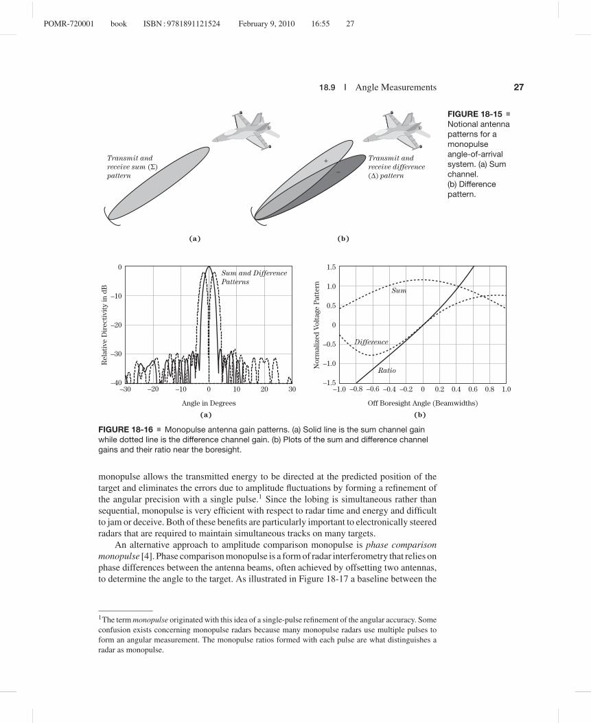
Monopulse is a simultaneous lobing technique that was developed to overcome theshortcomings of sequential lobing and conical scanning [13]. Monopulse antennas weredescribed in Chapter 9. In an amplitude comparison monopulse radar system, a pulse istransmitted directly at the predicted position of the target, and the target echo is receivedwith two squinted beams (“split beams”). Figures 18-15 and 18-16 illustrate the transmitand difference antenna patterns for a single-dimensional monopulse. The angle of arrival ofthe target is typically estimated with the in-phase part (i.e., the real part) of the monopulseratio, which is formed by dividing the difference of the two received signals by theirsum (see Figure 18-16). When tracking in azimuth and elevation, four beams are usedfor receive, and two monopulse ratios are typically formed. The simultaneous lobing of

FIGURE 18-14Conical sequentiallobing illustration.

Echo power vs. scan position

(a) (b)



Transmit and

receive sum (Σ)pattern

Transmit and

receive difference

(Δ) pattern

(a) (b)

+

–

FIGURE 18-15Notional antennapatterns for amonopulseangle-of-arrivalsystem. (a) Sumchannel.(b) Differencepattern.

(a)

Angle in Degrees

Sum and Difference

Patterns

Sum

Difference

Ratio

Rel

ativ

e D

irec

tivi

ty in

dB

–30 –20 –10 0 10 20 30–40

–30

–20

–10

0

(b)

Off Boresight Angle (Beamwidths)

Nor

mal

ized

Vol

tage

Pat

tern

–1.0 –0.8 –0.6 –0.4 –0.2 0.40.20 0.6 0.8 1.0–1.5

–1.0

–0.5

0

0.5

1.0

1.5

FIGURE 18-16 Monopulse antenna gain patterns. (a) Solid line is the sum channel gainwhile dotted line is the difference channel gain. (b) Plots of the sum and difference channelgains and their ratio near the boresight.

monopulse allows the transmitted energy to be directed at the predicted position of thetarget and eliminates the errors due to amplitude fluctuations by forming a refinement ofthe angular precision with a single pulse.1 Since the lobing is simultaneous rather thansequential, monopulse is very efficient with respect to radar time and energy and difficultto jam or deceive. Both of these benefits are particularly important to electronically steeredradars that are required to maintain simultaneous tracks on many targets.

An alternative approach to amplitude comparison monopulse is phase comparisonmonopulse [4]. Phase comparison monopulse is a form of radar interferometry that relies onphase differences between the antenna beams, often achieved by offsetting two antennas,to determine the angle to the target. As illustrated in Figure 18-17 a baseline between the

1The term monopulse originated with this idea of a single-pulse refinement of the angular accuracy. Someconfusion exists concerning monopulse radars because many monopulse radars use multiple pulses toform an angular measurement. The monopulse ratios formed with each pulse are what distinguishes aradar as monopulse.



Target

Plane wave approximationin far-field where R >> l. R

...

...

q

q

d

dsinq

FIGURE 18-17 Geometry of phase comparison monopulse. The displacement distanced between the antennas causes different path lengths to the target, which gives rise to adifference in phase of the return echo between the two beams. The target is assumed to befar enough away that the far-field approximation applies.

two beam phase centers creates a path length difference, dsin θ , to the target, which resultsin a phase difference in the signals. An important practical limitation in AOA measurementusing phase comparison monopulse is that, to prevent ambiguity in the estimated direction,the target angle and antenna baseline separation must meet the requirement [13]

|sin θ | <λ

8d(18.62)

Both monopulse and centroiding are used for AOA estimation in modern radar sys-tems. Implementing a monopulse AOA system is more expensive than implementing acentroiding AOA system. However, the time occupancy requirements of electronicallyscanned radars for multiple target tracking dictate the use of monopulse AOA estimation.In the remainder of this section, centroiding and monopulse AOA estimation are discussed.

18.9.1 Angle Centroiding for Scanning Radars

When considering the AOA estimation method for a rotating radar, centroiding should bethe first consideration. The estimation error of an angle centroider depends on the single-pulse SNR, the number of pulses transmitted within the antenna beamwidth, the antennagain pattern, and target fluctuation model. Two basic approaches to AOA centroiding arethe binary integration approach [14] and the ML approach [15]. The binary integrationapproach is motivated by the need to limit memory and processing in real-time radarsystems, while the ML approach is motivated by the need for more accurate estimation.However, studies have found that the AOA estimation of binary integration can approachthe CRLB for sufficiently high SNR and targets with rather stable radar cross sections.For Swerling targets, the CRLB for the AOA has the following form [14,16]

σ 2θ = θ2

3

N · SNR · α2(18.63)



N1 N0

–1

+1

w(k)

k

N0 N1

FIGURE 18-18Weights of a binaryBernstein estimatorfor angle-of-arrivalcentroiding.

where θ is the AOA, θ3 is the 3 dB beamwidth of the antenna pattern, N is the number ofpulses in the azimuth interval, and α is a constant that depends on the ratio of the azimuthobservational interval and the 3 dB antenna beamwidth. For a large azimuth observationinterval, α ≈ 0.339. While the performance of a centroider depends on many parameters,an AOA centroider can be expected to achieve σθ ≈ θ3

/10, where σθ is the standard

deviation of the error in the AOA estimate.In the binary integration approach, the samples of the matched filter output are quan-

tized to 0 or 1. For a given scan of the radar by the target, an AOA estimate can be producedby taking a simple average of the angle of the antenna boresight at the first detection of thetarget (i.e., the leading edge) and the angle of the antenna boresight at the final detectionof the target (i.e., the trailing edge). For targets with very stable echoes, this simple ap-proach performs reasonably well. However, for targets with fluctuating amplitudes, a bettermethod is needed. An improved approach is represented by the Bernstein estimator [14] inwhich the quantized detections are convolved with the weights shown in Figure 18-18. TheBernstein estimator uses N1 detection opportunities that occur as the antenna boresightscans toward the target and N1 detection opportunities that occur as the antenna boresightscans away from the target to reduce the sensitivity of the AOA estimate to amplitudefluctuations. The convolution of those detection opportunities with the Bernstein weightsgives rise to a zero crossing that corresponds to the AOA estimate of the target. The2N0 − 1 detection opportunities that occur when the antenna boresight is closely alignedwith the target are ignored by the Bernstein estimator as those samples provide very littleor no information concerning the AOA of the target. Typically, 2(N0 + N1) ≈ N . Optimalvalues for N0 and N1 are a function of the SNR of the target and the fluctuation model.Thus, the diversity of targets with respect to RCS and fluctuations make it impossible toachieve optimal AOA estimation without adaptation.

The ML approach to centroiding for AOA estimation involves formulating the mea-sured amplitude of the target echoes in terms of the antenna gain pattern and the angle ofthe target and computing the ML estimate of the target AOA. The target amplitude is typi-cally treated as a fixed, unknown quantity over the scan, which is a reasonable assumptionfor many targets if the pulses include at least 10 MHz of frequency agility.

18.9.2 Monopulse AOA Estimation

While most monopulse systems include AOA estimation to two angular coordinates,only monopulse processing in a single angular coordinate is considered in this section.The focus is on amplitude-comparison monopulse. Only the monopulse processing forRayleigh targets is considered here. The monopulse signals are formulated, and conven-tional monopulse processing is discussed first.



18.9.2.1 Single TargetUsing the notation in Section 18.3, equation (18.2) gives the sum signal for the monopulseprocessing, while the vertical difference signal is given by

d(t) = 2

√Pt

(4π)3

Gtλ

R2AG�(θ, ψ)G�V (θ, ψ)p(t) cos(ωct + ωd t + φ) + wd(t) (18.64)

where G�(θ, ψ) denotes the voltage gain of the antenna in the sum channel at (θ, ψ),G�V (θ, ψ) denotes the voltage gain of the antenna in the vertical difference channel at(θ, ψ), (θ, ψ) denotes the angular location of the target relative to antenna boresight, andwd(t) denotes the receiver noise in the vertical difference channel. A similar difference sig-nal will also be received for the horizontal coordinate. Note that “vertical” and “horizontal”are used to denote the two orthogonal coordinates of the radar. These differ from the localhorizontal and vertical if the antenna boresight is tilted out of the horizontal plane.

Monopulse is implemented slightly differently in phased array radars. In a phasedarray radar, two beamforming networks (three networks for monopulse in two angles)are used to simultaneously form sum and difference beams. The sum pattern as given inSection 18.3 may be used for transmit and receive in the sum channel, while the differencepattern may be the result of subtracting two beams, each formed with one-half of the array.Ignoring the Doppler and straddle losses, the in-phase and quadrature components of thesum (sI and sQ) signal and difference (dI and dQ) signal are given by

sI = α cos φ + ws I sQ = α sin φ + ws Q

dI = αη cos φ + wd I dQ = αη sin φ + wd Q(18.65)

where κ is a constant that depends on the target amplitude, system gain, and transmitpower and

α = κG�(θ, ψ), η = G�V (θ, ψ)

G�(θ, ψ), (18.66)

ws I ∼ N(0, σ 2

s

), ws I ∼ N

(0, σ 2

s

), wd I ∼ N

(0, σ 2

d

), wd Q ∼ N

(0, σ 2

d

)The receiver errors in the sum and difference channels are typically uncorrelated except

for a possible real-valued correlation or E(ns I nd I ) = E(ns Qnd Q) = ρσdσs [13]. Sincethe parameter η defines an off-boresight angle θ, η is referred to as the AOA parameter.Thus, monopulse processing involves the estimation of η and using the estimate of η tocompute the AOA relative to the antenna boresight.

In a typical monopulse system, the AOA with respect to the antenna boresight isapproximated by

θ ≈ θ3

kmη (18.67)

where 1 < km < 2 and θ3 is the 3 dB beamwidth of the antenna pattern. The linearapproximation to the monopulse error function is usually appropriate for −θ3

/2 ≤ θ ≤

θ3/

2. Denoting s = sI + jsQ and d = dI + jdQ, the in-phase and quadrature parts of themonopulse ratio are given by

yI = Re(

d

s

)= dI sI + sQdQ

s2I + s2

Q

, yQ = Im(

d

s

)= dQsI − dI sQ

s2I + s2

Q

(18.68)



Typically, yI is taken as the estimate of the direction on arrival (DOA), which gives theAOA estimate as

θ = θ3

km

(yI − ρ

σd

σs

)(18.69)

The variance of yI is often reported in the literature [13] as

σ 2yI

≈ 1

2 · SNR

[σ 2

d

σ 2s

+ η2 − 2ρσd

σs

], SNR > 13 dB (18.70)

where SNR is the signal-to-noise of the sum channel signal. Estimates of the variance ofyI are often computed by setting η = yI . An estimate of the variance of the AOA is thengiven by

σ 2θ

≈ θ23

k2m

σ 2yI

≈ θ23

2k2mSNR

[σ 2

d

σ 2s

+ y2I − 2ρ

σd

σs

], SNR > 13 dB (18.71)

Several authors have shown that yI is a notably biased2 estimate of the DOA atmoderate and low SNR. The bias is often reported in the literature [13] as

E(yI ) − η =(

ρσd

σs− η

)exp(−SNR) (18.72)

Seifer showed in [17] that this is an optimistic assessment of the bias because the measuredamplitude of the sum signal is subjected to a threshold test prior to monopulse processing.

For a Rayleigh target with real uncorrelated receiver errors, the joint PDF of thein-phase and quadrature parts of the monopulse ratio is given by

pyI ,yQ

(yI , yQ

∣∣SNRobs) = pyI ( yI |SNRobs) pyQ

(yQ

∣∣SNR0)

(18.73)

where SNRobs is the observed SNR α2η2/σ 2

d and

pyI (yI |SNRobs) = N

(SNR · η + ρσdσ

−1s

SNR + 1,

γ

2SNRobs

)

pyQ (yQ |SNRobs) = N(

0,γ

2SNRobs

)(18.74)

γ =[

σ 2d

σ 2s

(1 − ρ2

SNR + 1

)+ SNR · η

(η − 2ρσdσ

−1s

)SNR + 1

]

The notation N(μ, σ 2) denotes a normal (Gaussian) distribution with mean μ and varianceσ 2. Thus, yI and yQ are conditionally Gaussian, independent random variables. Note thatequation (18.74) shows that even for ρ = 0, yI is a notably biased observation of the DOAη for values of SNR less than about 13 dB.

2Notably biased estimate is used here to denote an estimate with bias greater than 5% of the true value.



Let yI denote the mean of yI given SNRobs. Then, for N independent samples orpulses, the ML estimate of yI is given by

yI = 1

NY N

N∑k=1

SNRobsk yIk , YN = 1

N

N∑k=1

SNRobsk (18.75)

where SNRobsk and yIk denote the observed SNR and in-phase monopulse ratio for pulsek, respectively. Thus, the estimate yI is a “power” or “energy” weighted sum of the Nmonopulse ratios. Since the yI k are Gaussian random variables, yI is the minimum varianceestimate of yI and a Gaussian random variable with variance given by

σ 2yI

= γ

2NY N(18.76)

where γ was defined in equation (18.74). However, note that yI being the minimumvariance estimate of yI does not imply that yI is the minimum variance estimate of η

[6]. For target tracking, an estimate of the variance σ 2yI

is found by setting η = yI andSNR = YN − 1 in p, resulting in

σ 2yI

= 1

2NY N

[σ 2

d

σ 2S

(1 − ρ2

YN

)+

(1 − 1

YN

)yI

(yI − 2ρσdσ

−1S

)](18.77)

Since the yI k are Gaussian, σ 2yI

is the conditional CRLB for yI given {SNRobsk }Nk=1

The term conditional here is used to denote the fact that the CRLB is developed withthe amplitude-conditioned PDF. While σ 2

yIprovides the variance of yI for real-time or

actual tracking, σ 2yI

cannot be used for performance prediction because it is a functionof {SNRobsk }N

k=1, which are measured quantities. The modified Cramer-Rao lower bound(MCRLB) [18], while somewhat looser than the CRLB, can be used for performanceprediction. The MCRLB of yI is given by

σ 2yI

≥ J (yI ) = p

2N (SNR + 1)(18.78)

18.9.2.2 Multiple Unresolved TargetsConventional monopulse processing is based on the assumption that each observationincludes a single resolved object. When measurements of two closely spaced objects aremade and conventional monopulse processing is employed, the resulting AOA measure-ment may not reflect the existence of two targets. Since the position and velocity estimatesof a target determine the association of any subsequent measurements to the target, failureto detect the presence of the interference of a second target and address it in the DOAestimation can be catastrophic to the performance of the tracking algorithm. For two un-resolved Rayleigh targets, the in-phase and quadrature parts of the sum (sI and sQ) and(dI and dQ) difference signals are given by [19]

sI = α1 cos φ1 + α2 cos φ2 + ws I , sQ = α1 sin φ1 + α2sinφ2 + ws Q

dI = α1η1 cos φ1 + α2η2 cos φ2 + wd I , dQ = α1η1 sin φ1 + α2η2sinφ2 + wd Q

(18.79)where ηi is the DOA parameter for target i. With SNRi denoting the average SNR fortarget i, the joint PDF of the in-phase and quadrature parts of the monopulse ratio for



uncorrelated receiver errors is again given by equation (18.73), but now with

pyI ( yI |SNRobs) = N(

SNR1η1 + SNR2η2

SNR1 + SNR2 + 1,

κ

2SNR0

)pyQ

(yQ

∣∣SNRobs) = N

(0,

qκ

2SNR0

)· (18.80)

κ =[

σ 2d

σ 2s

+ SNR1η21 + SNR2η

22 + SNR1SNR2(η1 − η2)

2

SNR1 + SNR2 + 1

]Thus, yI and yQ are conditionally Gaussian, independent random variables. Note thatequation (18.80) shows that the mean of yI is a power or energy weighted average of theDOAs of the two targets. With yI denoting the mean of yI given SNR0, the ML estimateof yI for N independent pulses is given by equation (18.75). Since the yIk are Gaussianrandom variables, yI is the minimum variance estimate of yI and a Gaussian randomvariable with variance given by

σ 2yI

= κ

2NYN(18.81)

The MCRLB of yI is given by

σ 2yI

≥ J (yI ) = κ

2N (SNR1 + SNR2 + 1)(18.82)

Figure 18-19 gives a comparison of the MCRLBs of yI for a single target and two un-resolved, equal-amplitude targets versus the total SNR in a single frequency (i.e., N = 1).To obtain yI = 0 in both cases, the single target was set at the antenna boresight, and thetwo targets were situated symmetrically about the boresight (i.e., η1 = −η2) and separatedby one-half of a beamwidth by setting η1 = 0.4 for km = 1.6. Figure 18-19 shows that atotal SNR of 14 dB gives a MCRLB of 0.02 for the single-target case and 0.095 for the two-target case. This figure also shows that doubling the energy in a single-frequency waveformto obtain a total SNR of 17 dB gives an MCRLB of 0.01 for the single-target case and 0.09for the two-target case. Thus, doubling the energy in a single-frequency pulse gives only a

06 8 10 12 14 16 18 20 22 24

0.02

0.04

0.06

0.08

0.10

0.12

0.14

0.16

Total Signal−to−noise Ratio (dB)

Mod

ifie

d C

RLB

Two Unresolved Targets

Single Resolved Target

FIGURE 18-19MCRLBs of yI for asingle pulse andsingle target at theboresight and twotargets separated byone-half beamwidthand symmetricabout the boresight.



small reduction in the MCRLB for the two-target case. However, if the energy in the pulseis doubled and a second frequency is added so that two independent observations of theunresolved targets are obtained, the MCRLB would be reduced by about 50 percent be-cause the errors are Gaussian (not shown in figure). Therefore, frequency agility is criticalto improving the monopulse angle estimation when two unresolved targets are present.

The failure to detect the presence of the interference of a second target can be catas-trophic to the performance of the tracking algorithm. A generalized likelihood ratio test(GLRT) for detection of the presence of unresolved Rayleigh targets is developed in [3].Waveform design and antenna boresight pointing for AOA estimation of two unresolvedRayleigh targets with a monopulse radar is addressed further in [19–21].

18.10 COORDINATE SYSTEMS

A radar system measures target position in spherical coordinates relative to the boresightof the radar antenna: range, R, azimuth angle, θ , and elevation angle, φ. These two anglecoordinates are measured in orthogonal planes in a coordinate system centered on theantenna. If the x direction is the “horizontal” dimension of the antenna, the y directionis the “vertical” dimension of the antenna, and the z dimension is the normal to theantenna face (the boresight direction in a mechanically-scanned antenna), then elevationis measured in the vertical y-z plane containing the radar boresight, while azimuth ismeasured in the horizontal x-z plane containing the boresight. The measurement errors inthese dimensions are generally independent of one another.

Frequently it is the case that it is desirable to track a target in a different coordinatesystem, typically a Cartesian (x-y-z) system centered at the radar platform or some otherconvenient reference point. The transformation from the spherical measurement coordi-nates back to antenna-centered Cartesian coordinates with the same origin is given by(18.83) and illustrated in Figure 18-20.

x = R cos θ sin φ

y = R sin θ sin φ (18.83)

z = R cos θ

FIGURE 18-20Spherical andCartesianrepresentations of athree-dimensionalvector.

z

x

yy0

x0

z0

f0

q0

R Cartesian:

[xyz

]=

[R cos(θ) sin(φ)

R sin(θ) sin(φ)

R cos(φ)

]

Polar:

R =√

x2 + y2 + z2

θ = tan−1

(y

x

)φ = cos−1

(z√

x2 + y2 + z2

)


18.12 References 35

Equation (18.83) shows that measurement errors in Cartesian coordinates are a non-linear combination of the spherical coordinate errors. Consequently, the errors in the threeCartesian coordinates are coupled: the error in x is not independent of the error in y andso forth. This complicates the design and analysis of optimal tracking algorithms [22].In practice, the transformation of the uncertainty model in the measurement frame to thetrack filter reference frame is typically accomplished by linearizing the model in equation(18.83) at the current estimates of R, θ , and ϕ.

The antenna-centered coordinates can in turn be rotated and translated into alternativeCartesian systems, for instance into coordinates aligned with the platform flight path, orto East-North-Up coordinates. Coordinate systems and coordinate conversion are a majortopic in track filtering and are addressed further in Chapter 19.

18.11 FURTHER READING

Additional material and alternative presentations on radar measurement accuracy maybe found in several sources. A description of number of practical approaches in radarmeasurement can be found in Barton and Ward’s handbook [6]. Peebles [4] and Raemer[23] provide extensive theoretical results and derivations in radar measurement theory.A good introduction to radar system design and performance analysis is provided by theclassic text [24]. Detailed background on the theory of measurement in the presence ofnoise is provided in the well-known book [25]. A popular forum for publication of currentresearch in this area is the IEEE Transactions on Aerospace Systems.

18.12 REFERENCES

[1] Richards, M.A., Fundamentals of Radar Signal Processing, McGraw-Hill, New York, 2005.

[2] Blair, W.D., and Keel, B.M., “Radar Systems Modeling for Target Tracking,” in Multitarget-Multisensor Tracking: Advanced and Applications, Vol. III, Ed. Y. Bar-Shalom and W.D.Blair, Artech House, Dedham, MA, 2000.

[3] Kay, S.M., Fundamentals of Statistical Signal Processing, Vol. 1: Estimation Theory, Prentice-Hall, Upper Saddle River, NJ, 1993.

[4] Peebles Jr., P.Z., Radar Principles, Wiley, New York, 1998.

[5] Levanon, N., Radar Principles, Wiley, New York, 1988.

[6] Barton, D.K., and Ward, H.R., Handbook of Radar Measurement, Artech House, Dedham,MA, 1984.

[7] Trunk, G.V., “Range Resolution of Targets Using Automatic Detectors,” IEEE Trans.Aerospace and Electronic Systems, vol. AES-14, no. 5, pp. 750–755, Sept. 1978.

[8] Trunk, G.V., “Range Resolution of Targets,” IEEE Trans. Aerospace and Electronic Systems,vol. AES-20, no. 6, pp. 789–797, Nov. 1984.

[9] Cook, C.E., and Bernfeld, M., Radar Signals: An Introduction to Theory and Application,Artech House, Norwood, MA, 1993.

[10] Jacobsen, E., and Kootsookos, P., “Fast Accurate Frequency Estimators,” IEEE SignalProcessing Magazine, pp. 123–125, May 2007.

[11] Doviak, R.J., and Zurnic, D.S., Doppler Radar and Weather Observations, 2d ed., AcademicPress, San Diego, 1993.



[12] Blair, W.D., and Brandt-Pearce, M., “Estimation and Discrimination for Swerling Targets,”Proceedings Twenty-Eighth Southeastern Symposium on System Theory, 1996, pp. 280–284,March 31–April 2, 1996.

[13] Sherman, S.M., Monopulse Principles and Techniques, Artech House, Dedham, MA, 1984.

[14] Galati, G., and Struder, F.A., “Angular Accuracy of the Binary Moving Window RadarDetector,” IEEE Trans. Aerospace and Electronic Systems, vol. AES-18, no. 4, pp. 416–422,July 1982.

[15] Galati, G., and Struder, F.A., “Maximum Likelihood Azimuth Estimation Applied to SSR/IFFSystems,” IEEE Trans. Aerospace and Electronic Systems, vol. AES-26, no. 1, pp. 27–43,Jan. 1990.

[16] Swerling, P., “Maximum Angular Accuracy of a Pulsed Search Radar,” Proc. of the IRE,vol. 44, pp. 1145–1155, Sept. 1956.

[17] Seifer, A.D., “Monopulse-Radar Angle Measurement in Noise,” IEEE Trans. Aerospace andElectronic Systems, vol. AES-30, pp. 950–957, July 1994.

[18] Gini, F., Reggiannini, R., and Mengali, U., “The Modified CramePr-Rao Bound in VectorParameter Estimation,” IEEE Trans. on Communications, vol. 46, no. 1, pp. 52–60, Jan. 1998.

[19] Blair, W.D., and Brandt-Pearce, M., “Monopulse DOA Estimation of Two UnresolvedRayleigh Targets,” IEEE Trans. Aerospace and Electronic Systems, vol. AES-37, no. 2,pp. 452–469, Apr. 2001.

[20] Willett, P.D., Blair, W.D., and Zhang, X., “The Multitarget Monopulse CRLB for MatchedFilter Samples,” IEEE Trans. Signal Processing, vol. 55, no. 8, pp. 4183–4198, August2007.

[21] Zhang, X., Willett, P., and Bar-Shalom, Y., “Monopulse Radar Detection and Localizationof Multiple Unresolved Targets via Joint Bin Processing,” IEEE Trans. Signal Processing,vol. 53, no. 4., pp. 122–1236., Apr. 2005

[22] Brookner, E., Tracking and Kalman Filtering Made Easy, John Wiley & Sons, Hoboken, NJ,1998.

[23] Raemer, H.R., Radar Systems Principles, CRC Press, Boca Raton, FL, 1997.

[24] Barton, D.K., Radar System Analysis and Modeling, Artech, New York, 2005.

[25] Van Trees, H.L., Detection, Estimation, and Modulation Theory, John Wiley & Sons, Inc.,New York, 1968.

18.13 PROBLEMS

1. If every RF power measurement has a calibration uncertainty of 0.1 dB, discuss the relativeaccuracy of RF path calibration by separately calibrating individual components or doing asingle end-to-end calibration.

2. Show that the general centroid estimator in equation (18.35) is unbiased when estimating afixed parameter in of Gaussian noise. Is this result changed for a power law detector?

3. Show the steps in deriving the CRLB equation (18.23) for estimating a constant in independentGaussian noise.

4. Find the joint probability density function p(y1, . . . yN |m) for N observations yk = m + wk

of a constant m in independent Gaussian noise given a particular value of m. Determine themaximum likelihood estimate by solving for the argument of p(y1, . . . yN |m) that maximizesthe joint probability function. Determine if the maximum likelihood estimate is biased.

long

Cross-Out


18.13 Problems 37

5. Derive the CRLB for estimating the RCS for Swerling 2 target in the presence of independentGaussian noise using the distribution for the measured power given in equation (18.61).

6. For problem 4, show that the maximum likelihood estimator for the signal power is the samplemean.

7. Plot the CRLB of the weight sums of N monopulse ratios for a single versus the variousparameters in equation (18.78). Comment on the effects of parameters. For an ideal monopulsesystem, what would these parameter values be and what would the CRLB be?

8. What is the minimum SNR required in a 40 MHz bandwidth LFM radar to ensure a single-pulserange precision of 30 m?

9. Repeat problem 4 for an unmodulated CW pulse.

10. What is the minimum SNR required for an unbiased phase estimator must produce a minimumerror of 10 deg. for N = 1 and N = 10 pulses?

11. What is the value of the CRLB for frequency estimation for a radar with an SNR = 20 dB, apulse length of 10 μs, and N = 1 pulse? What is the value for N = 20 pulses?

12. Compute the RMS bandwidth of (a) a CW pulse with a rectangular envelop, and (b) an LFMchirp. For part (b), assume that the frequency spectrum of the chirp is rectangular. What arethe implications of the signal modulation bandwidth on the bound on time-delay measurementprecision?

13. Compute the RMS time duration of (a) a rectangular pulse, (b) a triangular pulse, and (c) halfcosine pulse envelope shape. What are the implications of the pulse shape on the bound onfrequency measurement precision?

14. Derive equations (18.26) and (18.27) assuming the signal mean time duration τ and meanbandwidth B are zero where

τ =

∞∫−∞

t |s(t)|2dt

∞∫−∞

|s(t)|2dtB =

∞∫−∞

2π f |S( f )|2df

∞∫−∞

|S( f )|2df

long

Inserted Text

the


38

chapter radar measurements - mers -- byu - news & · pdf file18.10 coordinate systems ......

Documents