chapter three continued annual demand - national grid plc

Chapter three continued Annual Demand

November 2016

GAS DEMAND FORECASTING METHODOLOGY DISCLAIMER

This document and this web site ("the Site") must be used in accordance with the following Terms and

Conditions that are governed by the law of and subject to the jurisdiction of England & Wales: This document is produced for the purpose of providing a general overview of the methodology National

Grid use to calculate peak day demand forecasts and load duration curves. This methodology is constantly evolving and therefore this report does not necessarily represent the exact processes in use at a particular time. All graphs and data are for illustration purposes only.

National Grid plc and members of the National Grid group of companies (the "Group") do not accept any liability for the accuracy of the information contained herein and, in particular neither National Grid or the

Group, or directors or employees of National Grid or the Group shall be under any liability for any error or misstatement or opinion on which the recipient of this document relies or seeks to rely other than fraudulent statements or fraudulent misrepresentation.

Whilst National Grid plc has taken all reasonable steps to ensure the accuracy of all the information in this document at the time of its inclusion, National Grid plc cannot accept responsibility for any loss or damage

resulting from any inadvertent errors or omissions appearing in this document and any visitor using information contained in this document does so entirely at their own risk.

You may not reproduce, modify or in any way commercially exploit any of the contents of this document, which shall include, but is not limited to, distributing any of the content of this document to third parties by you (including operating a library, archive or similar service).

National Grid plc reserves the right to modify, alter, delete and update at any time the contents of this document.

Copyright

Any and all copyright and all other intellectual property rights contained in this document and in any other Site content (including PDF documentation) belong to National Grid plc.

© 2016 National Grid plc, all rights reserved. You may not reproduce, modify or in any way commercially exploit any of the contents of this document which shall include, but is not limited to, distributing any of the content of this document to third parties by you (including photocopying and restoring

in any medium or electronic means and whether or not transiently or incidentally or operating a library, archive or similar service) without the written permission of National Grid plc except as permitted by law.

The trademarks, logos and service marks displayed on the document and on the Site are owned and registered (where applicable) by National Grid plc or its parent, subsidiary or affiliated companies. No rights or licence is granted or may be implied by their display in this document or on the Site.

Gas Demand Forecasting Methodology

Statement Contents

Chapter 1: Background 4 Chapter 2: Weather Concepts 10

Chapter 3: Annual Demand 14 Chapter 4: Daily Demand Modelling 18

Chapter 5: Simulation of Future Demand 22 Appendix 1: Weather 25 Appendix 2: Daily Demand modelling 31

Appendix 3: Load Duration Curve Production 36 Appendix 4: Extracts from Gas Transporter’s Licence 50

Appendix 5: References 51 Appendix 6: Data in the Public Domain 52 Appendix 7: Demand Data Definitions 53

Glossary 56

This report describes the methodology utilised by National Grid to produce forecasts of peak day gas demand and load duration curves. Chapters 1 – 5 deal with the concepts, while the Appendices 1 – 7 contain more technical details.

Day-ahead and within-day gas demand forecasting utilises a separate methodology, which is not covered in this report.

The forecasting methodology evolves over time in response to changes in the market, new technology and changing requirements. This document describes the processes used to produce National Grid’s 2016 demand forecasts. The original document was first published in November 2004.

Peak day and annual forecasts are published in the Ten Year Statement, while scenario assumptions are published in the UK Future Energy Scenarios Document. Additional forecasting and supply/demand modelling information is published in the winter and summer outlook documents.

All documents are available on the National Grid website, and the links can be found in Appendix 6.

Chapter one

Background

1.1 What is demand and why are forecasts produced?

Demand can be categorised in many different ways. NTS (National Transmission System) demand refers to the amount of gas used by gas consumers directly connected to the NTS, and includes most gas fired power stations and some large industrial units. LDZ (Local Distribution Zone) demand refers to the total amount of gas used by gas consumers connected to the gas distribution networks. This includes residential demand, and most commercial and industrial demand. Other elements of demand can sometimes include shrinkage (gas leaks, theft etc), European and Irish exports, and gas injected into storage. Demand can be represented in various ways, annually, daily or by load duration curve, where demand is ranked from highest to lowest. Load duration curves are explained in Chapter 5. Demand forecasts are used in a wide variety of contexts, some of which include: Safety Demand forecasts are used in the calculation of safety monitors, which are used to ensure sufficient gas is held in storage to underpin the safe operation of the NTS.

Security of Supply Demand forecasts are a key element of security of supply analyses such as that undertaken for the Winter Consultation and Winter Outlook Reports. The reports include detailed demand analysis with assumed supplies matched to them. The reports can be found at: www.nationalgrid.com/wor Licence Condition Annual demand forecasts for the next ten years are required by Standard Condition 25 of National Grid’s Gas Transporter Licence, and section O of the UNC. These forecasts are published annually in the Ten Year Statement, which can be found at: www.nationalgrid.com/gtys Investment Planning National Grid is required by its Gas Transporter Licence to develop the gas network so it can transport the gas demand on a 1 in 20 peak day. This term is explained later in Chapter 5. Operational Planning Demand and supply forecasts contribute to the safe, reliable and efficient operational planning of the NTS in advance. Pricing The demand forecasts are also used in the setting of prices that recover National Grid’s allowed revenue.

http://www.nationalgrid.com/wor

http://www.nationalgrid.com/gtys

Chapter one continued

Background

1.2 How are demand forecasts broken down?

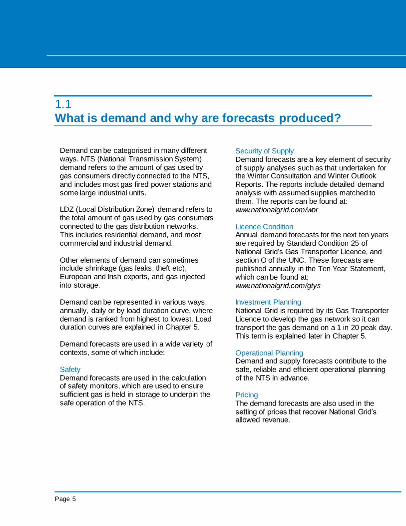
Demand forecasts are produced for each of the 13 local distribution zones (LDZ) as shown in Figure 1.1.

Figure 1.1 – UK Local Distribution Zones

Within each LDZ, each meter point or offtake from the network is categorised by how much gas it consumes, known as its load band. Load bands can be split into two discrete categories – Non daily metered (NDM) and daily metered (DM). Non daily metered load bands are offtakes where the meter is not read every day, such as residential properties, while some large industrial premises with much higher demand have their meters read daily. LDZ end users are categorised by how much gas they consume. Table 1.1 shows the different load bands connected to a distribution network.

Region: Code:

Scotland SC Northern NO North West NW North East NE East Midlands EM West Midlands WM Wakes North WN Wales South WS Eastern EA North Thames NT South East SE Southern SO South West SW


Statement

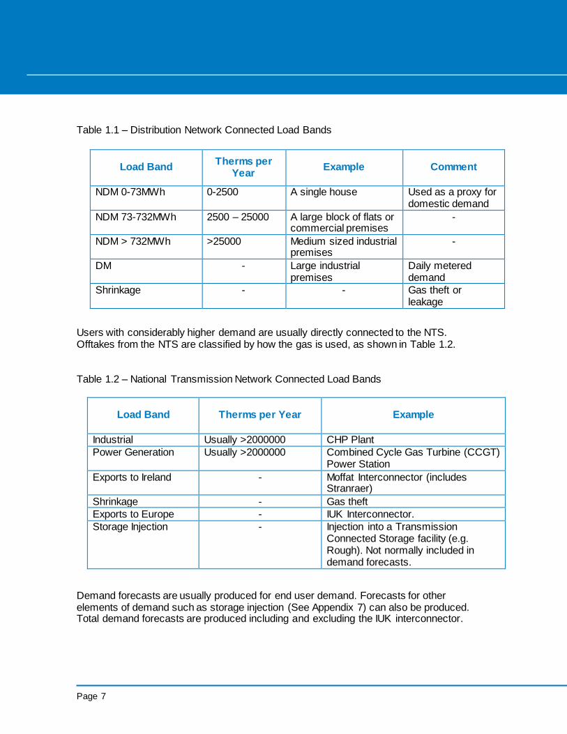
Table 1.1 – Distribution Network Connected Load Bands

Users with considerably higher demand are usually directly connected to the NTS. Offtakes from the NTS are classified by how the gas is used, as shown in Table 1.2.

Table 1.2 – National Transmission Network Connected Load Bands

Load Band

Therms per Year Example

Industrial Usually >2000000 CHP Plant

Power Generation Usually >2000000 Combined Cycle Gas Turbine (CCGT) Power Station

Exports to Ireland - Moffat Interconnector (includes Stranraer)

Shrinkage - Gas theft

Exports to Europe - IUK Interconnector.

Storage Injection - Injection into a Transmission Connected Storage facility (e.g. Rough). Not normally included in demand forecasts.

Demand forecasts are usually produced for end user demand. Forecasts for other elements of demand such as storage injection (See Appendix 7) can also be produced. Total demand forecasts are produced including and excluding the IUK interconnector.

Load Band

Therms per Year

Example Comment

NDM 0-73MWh 0-2500

A single house Used as a proxy for domestic demand

NDM 73-732MWh 2500 – 25000 A large block of flats or commercial premises

-

NDM > 732MWh >25000 Medium sized industrial premises

-

DM - Large industrial premises

Daily metered demand

Shrinkage - - Gas theft or leakage

Chapter one continued

Background

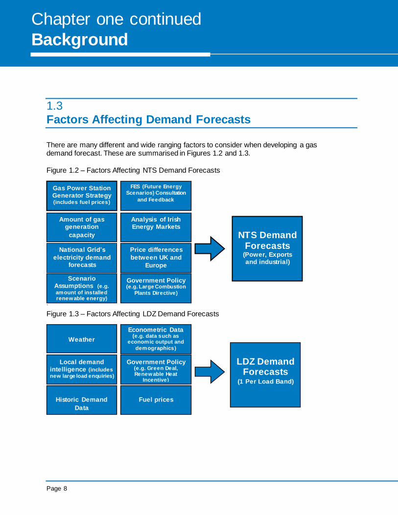
1.3 Factors Affecting Demand Forecasts

There are many different and wide ranging factors to consider when developing a gas demand forecast. These are summarised in Figures 1.2 and 1.3.

Figure 1.2 – Factors Affecting NTS Demand Forecasts

`

Figure 1.3 – Factors Affecting LDZ Demand Forecasts

Gas Power Station Generator Strategy (includes fuel prices)

Government Policy (e.g. Large Combustion

Plants Directive)

Analysis of Irish Energy Markets

National Grid’s

electricity demand forecasts

FES (Future Energy

Scenarios) Consultation

and Feedback

Scenario Assumptions (e.g.

amount of installed renewable energy)

Price differences

between UK and

Europe

Amount of gas generation

capacity

NTS Demand

Forecasts (Power, Exports and industrial)

Weather

Local demand intelligence (includes

new large load enquiries)

Historic Demand

Data

Fuel prices

Econometric Data (e.g. data such as

economic output and

demographics)

Government Policy (e.g. Green Deal, Renewable Heat

Incentive)

LDZ Demand

Forecasts (1 Per Load Band)


Statement

Variability in day to day demand tends to be driven by weather and fuel prices. Weather is the main driver for LDZ connected NDM demand, while the main driver for NTS power generation demand is relative fuel prices. Demand for other NTS connected loads and DM LDZ demand tend to be less variable. Assumptions behind the forecasts can be found in our Future Energy Scenarios document.1

1 http://fes.nationalgrid.com/

Chapter two

Weather Concepts


Statement

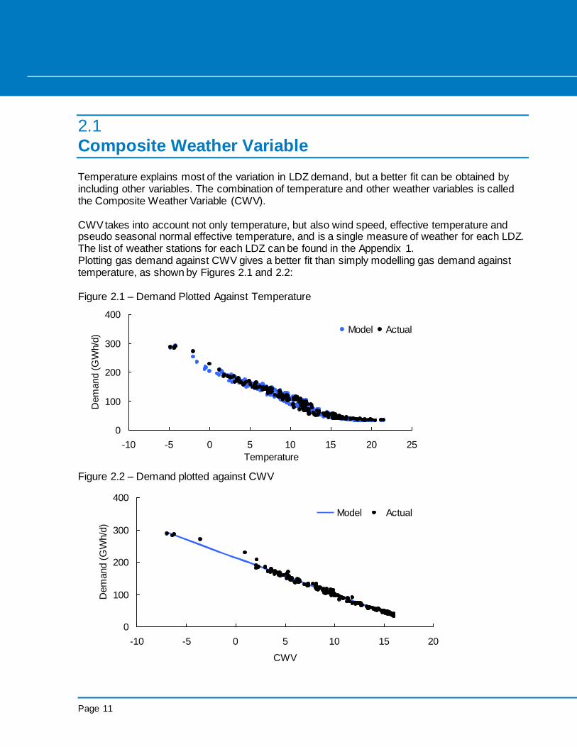
2.1 Composite Weather Variable Temperature explains most of the variation in LDZ demand, but a better fit can be obtained by including other variables. The combination of temperature and other weather variables is called the Composite Weather Variable (CWV). CWV takes into account not only temperature, but also wind speed, effective temperature and pseudo seasonal normal effective temperature, and is a single measure of weather for each LDZ. The list of weather stations for each LDZ can be found in the Appendix 1. Plotting gas demand against CWV gives a better fit than simply modelling gas demand against temperature, as shown by Figures 2.1 and 2.2: Figure 2.1 – Demand Plotted Against Temperature

0

100

200

300

400

-10 -5 0 5 10 15 20 25

Temperature

Dem

and (

GW

h/d

)

Model Actual

Figure 2.2 – Demand plotted against CWV

0

100

200

300

400

-10 -5 0 5 10 15 20

CWV

Dem

and (

GW

h/d

)

Model Actual

Chapter two continued

Weather Concepts

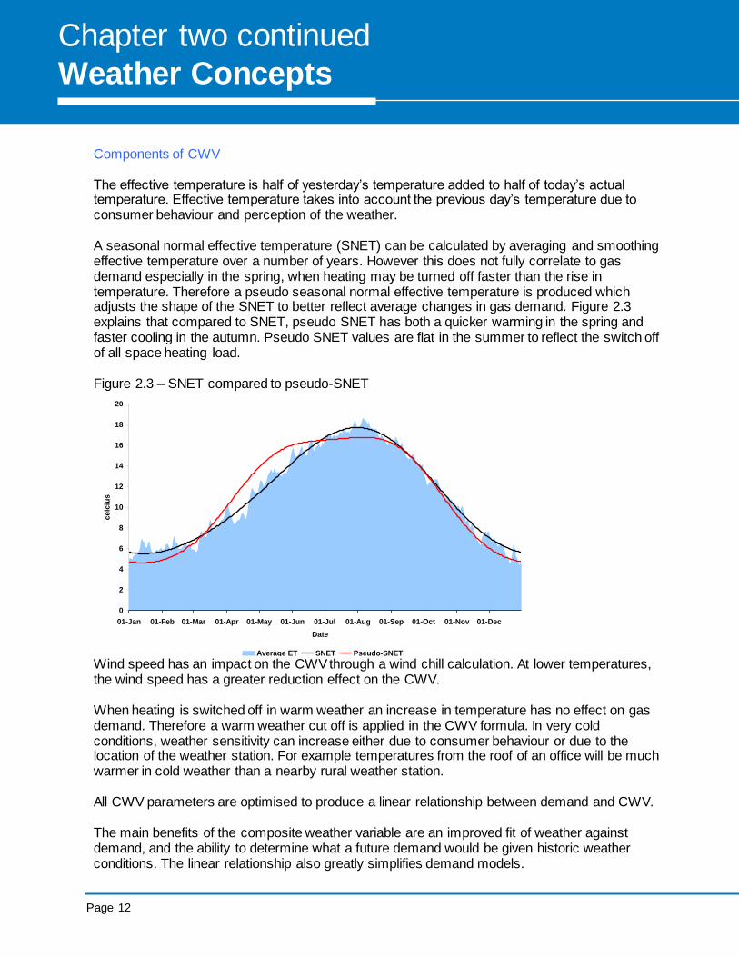
Components of CWV The effective temperature is half of yesterday’s temperature added to half of today’s actual temperature. Effective temperature takes into account the previous day’s temperature due to consumer behaviour and perception of the weather. A seasonal normal effective temperature (SNET) can be calculated by averaging and smoothing effective temperature over a number of years. However this does not fully correlate to gas demand especially in the spring, when heating may be turned off faster than the rise in temperature. Therefore a pseudo seasonal normal effective temperature is produced which adjusts the shape of the SNET to better reflect average changes in gas demand. Figure 2.3 explains that compared to SNET, pseudo SNET has both a quicker warming in the spring and faster cooling in the autumn. Pseudo SNET values are flat in the summer to reflect the switch off of all space heating load. Figure 2.3 – SNET compared to pseudo-SNET

0

2

4

6

8

10

12

14

16

18

20

01-Jan 01-Feb 01-Mar 01-Apr 01-May 01-Jun 01-Jul 01-Aug 01-Sep 01-Oct 01-Nov 01-Dec

Date

ce

lciu

s

Average ET SNET Pseudo-SNET Wind speed has an impact on the CWV through a wind chill calculation. At lower temperatures, the wind speed has a greater reduction effect on the CWV. When heating is switched off in warm weather an increase in temperature has no effect on gas demand. Therefore a warm weather cut off is applied in the CWV formula. In very cold conditions, weather sensitivity can increase either due to consumer behaviour or due to the location of the weather station. For example temperatures from the roof of an office will be much warmer in cold weather than a nearby rural weather station. All CWV parameters are optimised to produce a linear relationship between demand and CWV. The main benefits of the composite weather variable are an improved fit of weather against demand, and the ability to determine what a future demand would be given historic weather conditions. The linear relationship also greatly simplifies demand models.


Statement

2.2 Seasonal Normal Weather and Weather Correction

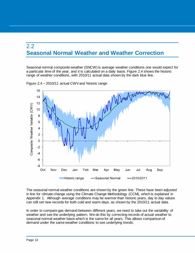
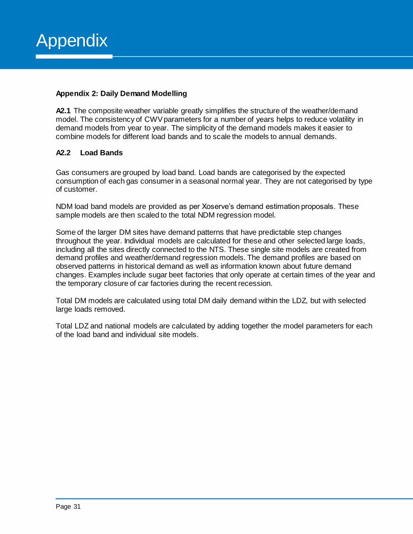
Seasonal normal composite weather (SNCW) is average weather conditions one would expect for a particular time of the year, and it is calculated on a daily basis. Figure 2.4 shows the historic range of weather conditions, with 2010/11 actual data shown by the dark blue line.

Figure 2.4 – 2010/11 actual CWV and historic range

The seasonal normal weather conditions are shown by the green line. These have been adjusted in line for climate change using the Climate Change Methodology (CCM), which is explained in Appendix 1. Although average conditions may be warmer than historic years, day to day values can still set new records for both cold and warm days, as shown by the 2010/11 actual data.

In order to compare gas demand between different years, we need to take out the variability of weather and see the underlying pattern. We do this by correcting records of actual weather to seasonal normal weather basis which is the same for all years. This allows comparison of demand under the same weather conditions to see underlying trends.

Chapter three Annual Demand


Statement

3.1

Annual LDZ Demand

An annual LDZ demand forecast must be produced before daily demands can be calculated. To produce detailed daily forecasts, we merge annual forecasts with weather models. This section gives an overview of the approach used to forecast annual demands. Annual demand is forecast for each load band within each LDZ. These are then aggregated to give total annual LDZ demand. Traditionally National Grid has produced a single forecast of annual gas demand based on analysis of history and views of the future incorporating forecasts of economic growth, industry intelligence about new developments, new technologies and new connections to the gas network. More recently, National Grid has adopted a scenario based approach for forecasting. The economic, technological and consumer landscapes are changing at an unprecedented rate. Against this backdrop it is impossible to forecast a single energy future over the long term. By providing a range of credible futures, we can be confident that the reality will be captured somewhere within that range. For more information on the assumptions behind National Grid’s scenarios, please refer to the Future Energy Scenarios (FES) document. The main inputs into LDZ demand models are historic demand data, information from distribution networks (exchanged under Section H of the UNC) and scenario assumptions. Adjustments are made for increased levels of insulation, appliance efficiency and the uptake of low carbon technologies. National Grid’s annual demand forecasts can be found in the FES document.2

2 www.nationalgrid.com/fes

Chapter three continued Annual Demand

3.2 Annual NTS Demand

There are relatively few NTS customers so these can all be forecast individually. Annual NTS modelling can be split into three distinct sections – power generation, industrial sites and exports. 3.2(A) Power Generation The power generation forecast consists of two main elements:

The amount of installed gas generation (total capacity) and;

How frequently this capacity is used. Information on gas generation capacity is combined from connections requests and load enquiries, with feedback received from National Grid’s annual FES3 consultation process and a range of commercial sources. The influence of the age of individual stations, generator portfolios, commercial arrangements, government policies and environmental legislation are taken into account when forecasting which power stations will be built or closed. Gas demand for power generation is extracted from a model which matches every power station’s output to electricity demand using a typical profile. This model utilises National Grid Electricity Transmission’s own electricity demand forecasts. The modelling process takes account of station specific operating assumptions, constraints, availability and costs, which are changed on a 3 month basis.

3.2(B) Exports Forecast flow rates to and from Europe via the Interconnector are based on historic flow patterns and an assessment of relative gas prices between Europe and the UK allowing for the seasonal price variation of gas prices.

Exports to Ireland are derived from a sector-based analysis of energy markets in Northern Ireland and the Republic of Ireland, including allowances for the depletion and development of indigenous gas-supplies, feedback from the FES consultation, commercial sources and regulatory publications.

3 The Future Energy Scenarios (FES) consultation replaces the previous TBE (Transporting Britain’s Energy). Some

documents may still refer to TBE.


Statement

3.2(C) Industrials

The production of forecasts within this sector is dependent on forecasts of individual new and existing loads based on recent demand trends, FES feedback, load enquiries and commercial sources.

3.2(D) Sensitivity Analysis Given the volatility seen in energy markets and other uncertainties, sensitivity analysis is carried out to look at a range of different demands. Along with the main demand forecasts, ‘high’ and ‘low’ cases are assessed for each component of the demand forecast.

Chapter four Daily Demand


Statement

4.1 LDZ Daily Demand Forecasts

This chapter deals with the conversion of total annual demand forecasts into daily forecasts. The first section of this chapter deals with LDZ annual demand, while the latter part deals with NTS demand.

There are two main components of LDZ demand: Non Daily Metered (NDM). These are sites where meters are not read on a daily basis, NDM demand accounts for most weather sensitive load. (See Table 1.1). NDM demand is calculated by subtracting daily metered (DM) demand and shrinkage from total LDZ demand. Daily Metered (DM). This refers to most industrial premises where meters are read (remotely) on a daily basis. As meters are read daily, some sites can be modelled individually to remove step changes from underlying demand. A sugar beet factory, for example usually only operates at certain times of the year. Such loads tend to be less weather related. In order to find the total LDZ daily demand given a CWV, a regression model is used. Historical weather and demand data is gathered to produce a model for each of the last three years. The LDZ models are calculated by using total daily demand within each LDZ4. Figure 4.1 – NDM Demand 2010/11

0

1000

2000

3000

4000

-5 0 5 10 15 20

CWV

GW

h/d

Actual - Weekday Model - WeekdayActual - Weekend or holiday Model - Weekend or holiday

Figure 4.1 shows the relationship between NDM demand and CWV. The chart shows a strong relationship between CWV and gas demand.

4 Large loads are removed as they are forecast separately.

Chapter four continued Daily Demand

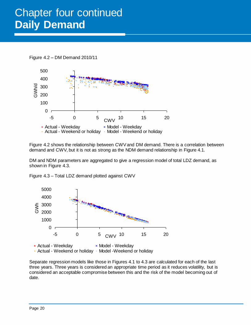
Figure 4.2 – DM Demand 2010/11

0

100

200

300

400

500

-5 0 5 10 15 20CWV

GW

h/d

Actual - Weekday Model - WeekdayActual - Weekend or holiday Model - Weekend or holiday

Figure 4.2 shows the relationship between CWV and DM demand. There is a correlation between demand and CWV, but it is not as strong as the NDM demand relationship in Figure 4.1.

DM and NDM parameters are aggregated to give a regression model of total LDZ demand, as shown in Figure 4.3.

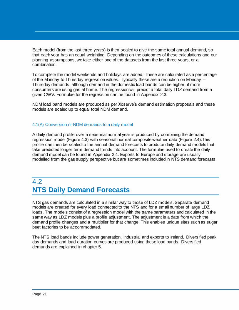
Figure 4.3 – Total LDZ demand plotted against CWV

0

1000

2000

3000

4000

5000

-5 0 5 10 15 20CWV

GW

h

Actual - Weekday Model - WeekdayActual - Weekend or holiday Model -Weekend or holiday

Separate regression models like those in Figures 4.1 to 4.3 are calculated for each of the last three years. Three years is considered an appropriate time period as it reduces volatility, but is considered an acceptable compromise between this and the risk of the model becoming out of date.


Statement

Each model (from the last three years) is then scaled to give the same total annual demand, so that each year has an equal weighting. Depending on the outcomes of these calculations and our planning assumptions, we take either one of the datasets from the last three years, or a combination. To complete the model weekends and holidays are added. These are calculated as a percentage of the Monday to Thursday regression values. Typically these are a reduction on Monday – Thursday demands, although demand in the domestic load bands can be higher, if more consumers are using gas at home. The regression will predict a total daily LDZ demand from a given CWV. Formulae for the regression can be found in Appendix 2.3. NDM load band models are produced as per Xoserve’s demand estimation proposals and these models are scaled up to equal total NDM demand.

4.1(A) Conversion of NDM demands to a daily model

A daily demand profile over a seasonal normal year is produced by combining the demand regression model (Figure 4.3) with seasonal normal composite weather data (Figure 2.4).This profile can then be scaled to the annual demand forecasts to produce daily demand models that take predicted longer term demand trends into account. The formulae used to create the daily demand model can be found in Appendix 2.4. Exports to Europe and storage are usually modelled from the gas supply perspective but are sometimes included in NTS demand forecasts.

4.2 NTS Daily Demand Forecasts NTS gas demands are calculated in a similar way to those of LDZ models. Separate demand models are created for every load connected to the NTS and for a small number of large LDZ loads. The models consist of a regression model with the same parameters and calculated in the same way as LDZ models plus a profile adjustment. The adjustment is a date from which the demand profile changes and a multiplier for that change. This enables unique sites such as sugar beet factories to be accommodated.

The NTS load bands include power generation, industrial and exports to Ireland. Diversified peak day demands and load duration curves are produced using these load bands. Diversified demands are explained in chapter 5.

Chapter five Simulation of Future Demand


Statement

5.1 How demand models are used

It is useful to understand what demand may be under different weather conditions. This is done by combining forecast daily demand models with historic weather. The results tell us what future demand may be if historic weather were to be repeated.

From these simulations we can apply statistical analysis to obtain 1 in 20 peak day demand forecasts and load duration curves. 5.1(A) Peak Day Demands

Peak day demand represents an extreme high level of demand. There are several methodologies for calculating peak day demand which all have different uses. Diversified peak day demand is the demand that could be expected for the whole country on a very cold day. It is calculated by fitting a statistical distribution to the highest demand day from each of the simulated gas supply years. Diversified demand is used for comparing with actual demand and for most operational and security planning. Undiversified demand is the peak day demand for each LDZ and NTS site added together. It is used where the location of capacity is important such as designing the network. The LDZ peaks are calculated using simulation methodology separately for each LDZ. NTS site peak demands are derived from a number of sources including historical demand, sold capacity, baseline capacity and new gas connection enquiries. Historically, the undiversified firm5 1 in 20 peak day demand was used to create network models6. Following exit reform all loads are now firm and so the undiversified peak is now much bigger. A realistic network model may not be obtained because there is not always enough supply available to provide a match. Instead, we now start with a diversified peak apportioned to each offtake and then stress test the model by increasing demands to obligated levels for sensitive parts of the network. There are two main causes of demand variation: weather and power generation. The diversified peak day methodology forecasts demand under extreme weather conditions. From 2012 it also includes the high sensitivity power generation forecasts. This is because when fuel prices favour coal, gas power stations provide the flexible generation. Base case forecasts will be low because it assumes high availability of other fuels. Any increase in electricity demand or decrease in availability of non-gas generation will result in a corresponding increase in gas generation. The

5 Firm demand is demand from gas consumers who have guaranteed capacity rights.

6 For network design.

Chapter five Simulation of Future Demand

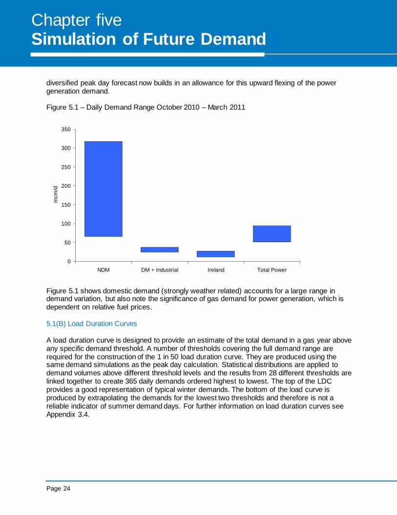
diversified peak day forecast now builds in an allowance for this upward flexing of the power generation demand. Figure 5.1 – Daily Demand Range October 2010 – March 2011

0

50

100

150

200

250

300

350

NDM DM + Industrial Ireland Total Power

mcm

/d

Figure 5.1 shows domestic demand (strongly weather related) accounts for a large range in demand variation, but also note the significance of gas demand for power generation, which is dependent on relative fuel prices. 5.1(B) Load Duration Curves A load duration curve is designed to provide an estimate of the total demand in a gas year above any specific demand threshold. A number of thresholds covering the full demand range are required for the construction of the 1 in 50 load duration curve. They are produced using the same demand simulations as the peak day calculation. Statistical distributions are applied to demand volumes above different threshold levels and the results from 28 different thresholds are linked together to create 365 daily demands ordered highest to lowest. The top of the LDC provides a good representation of typical winter demands. The bottom of the load curve is produced by extrapolating the demands for the lowest two thresholds and therefore is not a reliable indicator of summer demand days. For further information on load duration curves see Appendix 3.4.


Statement

Appendix

Appendix 1 Weather

A1.1 Composite Weather Variable

The Composite Weather Variable (CWV) is a daily weather variable created from 2-hourly temperatures and 4-hourly wind speeds. A separate composite weather variable is produced for each LDZ although the same weather station is sometimes used for more than one CWV. The national composite weather variable is a weighted average of the LDZ CWVs. The CWV is for a gas day, 5am to 5am7. The components of the composite weather variable are

1. Effective temperature (0.5 * today’s temperature + 0.5 * yesterday’s effective) 2. Pseudo seasonal normal effective temperature 3. Wind chill 4. Cold weather upturn 5. Summer cut-off

The pseudo seasonal normal effective temperature is the seasonal normal effective temperature adjusted to the profile of seasonal normal NDM demand. A composite weather variable is also used by Xoserve for demand estimation purposes and is described in Section H of the Uniform Network Code. There is no requirement for the same CWV to be used for demand estimation and demand forecasting. It may be that as the methodologies develop in the future different CWVs will be used for each task. However, at present it is more efficient to use the same composite weather definition. The composite weather variable parameters are calculated from historical weather and demand data. For demand estimation (and demand forecasting) they are recalculated at appropriate frequencies determined by the cross-industry Demand Estimation Sub Committee (DESC)

8. The

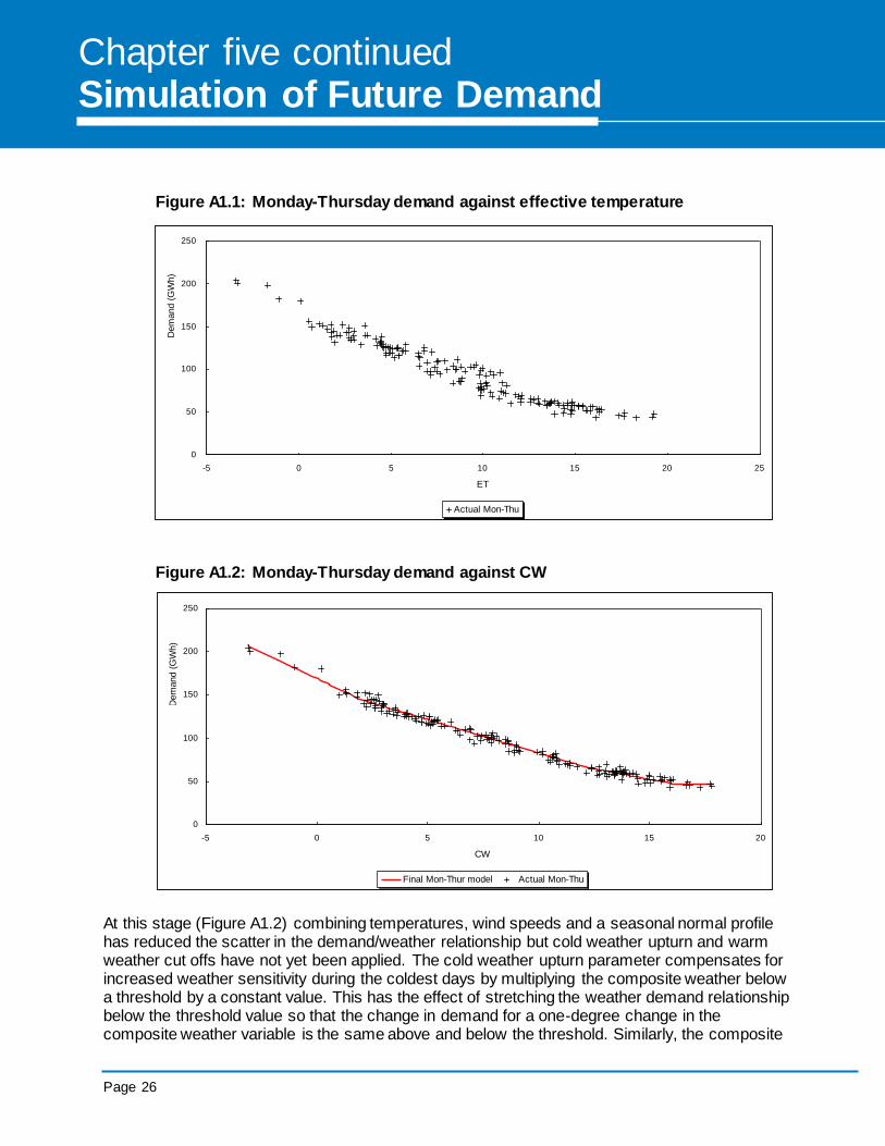
parameters are calculated in a number of steps, which ensure that changes to one parameter do not have an adverse effect on the fit of the whole model. It also enables different data to be used in different stages. The last CWV review was undertaken in 2014 and was overseen by DESC and its technical working group. For the most part, the update was based on 10 years of historic data from gas supply year 2004/05 to 2013/14. The cold weather upturn parameters were calculated using a longer history from 1996/97 onwards. This approach ensured that there was a reasonably sized historic dataset representing cold days. The following graphs illustrate how well the CWV improves the fit of the demand model.

7 Prior to 1 October 2015 the gas day was from 6am to 6am.

8 gasgovernance.co.uk/desc

Chapter five continued Simulation of Future Demand

Figure A1.1: Monday-Thursday demand against effective temperature

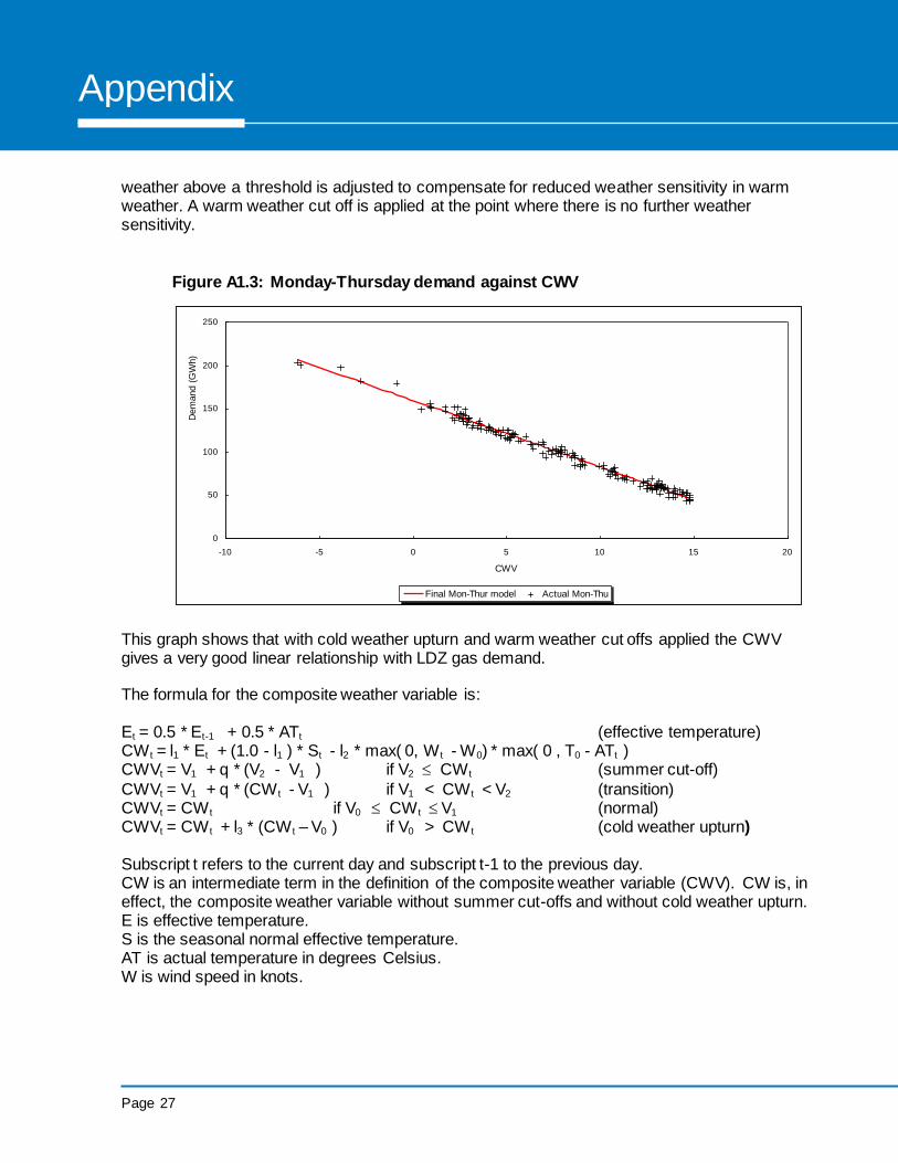
Figure A1.2: Monday-Thursday demand against CW

At this stage (Figure A1.2) combining temperatures, wind speeds and a seasonal normal profile has reduced the scatter in the demand/weather relationship but cold weather upturn and warm weather cut offs have not yet been applied. The cold weather upturn parameter compensates for increased weather sensitivity during the coldest days by multiplying the composite weather below a threshold by a constant value. This has the effect of stretching the weather demand relationship below the threshold value so that the change in demand for a one-degree change in the composite weather variable is the same above and below the threshold. Similarly, the composite

0

50

100

150

200

250

-5 0 5 10 15 20 25

ET

Maxim

um

Pote

ntial D

em

and (

GW

h)

Actual Mon-Thu

0

50

100

150

200

250

-5 0 5 10 15 20

CW

Maxim

um

Pote

ntial D

em

and (

GW

h)

Final Mon-Thur model Actual Mon-Thu


Statement

Appendix

weather above a threshold is adjusted to compensate for reduced weather sensitivity in warm weather. A warm weather cut off is applied at the point where there is no further weather sensitivity.

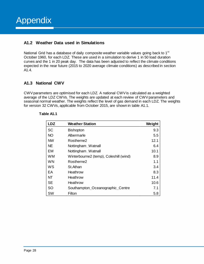
Figure A1.3: Monday-Thursday demand against CWV

This graph shows that with cold weather upturn and warm weather cut offs applied the CWV gives a very good linear relationship with LDZ gas demand. The formula for the composite weather variable is: Et = 0.5 * Et-1 + 0.5 * ATt (effective temperature) CW t = l1 * Et + (1.0 - l1 ) * St - l2 * max( 0, W t - W0) * max( 0 , T0 - ATt ) CWVt = V1 + q * (V2 - V1 ) if V2 CW t (summer cut-off)

CWVt = V1 + q * (CW t - V1 ) if V1 < CW t < V2 (transition) CWVt = CW t if V0 CW t V1 (normal) CWVt = CW t + l3 * (CW t – V0 ) if V0 > CW t (cold weather upturn)

Subscript t refers to the current day and subscript t-1 to the previous day. CW is an intermediate term in the definition of the composite weather variable (CWV). CW is, in effect, the composite weather variable without summer cut-offs and without cold weather upturn. E is effective temperature. S is the seasonal normal effective temperature. AT is actual temperature in degrees Celsius. W is wind speed in knots.

0

50

100

150

200

250

-10 -5 0 5 10 15 20

CWV

Maxim

um

Pote

ntial D

em

and (

GW

h)

Final Mon-Thur model Actual Mon-Thu

Appendix

A1.2 Weather Data used in Simulations

National Grid has a database of daily composite weather variable values going back to 1st October 1960, for each LDZ. These are used in a simulation to derive 1 in 50 load duration curves and the 1 in 20 peak day. The data has been adjusted to reflect the climate conditions expected in the near future (2015 to 2020 average climate conditions) as described in section A1.4.

A1.3 National CWV

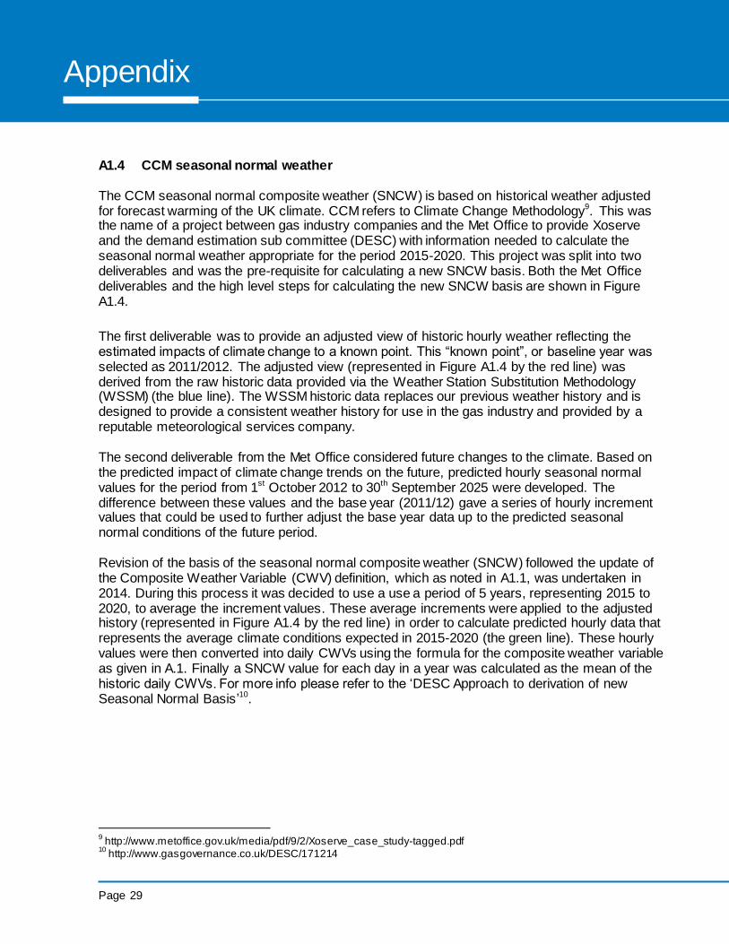
CWV parameters are optimised for each LDZ. A national CWV is calculated as a weighted average of the LDZ CWVs. The weights are updated at each review of CWV parameters and seasonal normal weather. The weights reflect the level of gas demand in each LDZ. The weights for version 32 CWVs, applicable from October 2015, are shown in table A1.1. Table A1.1

LDZ Weather Station Weight

SC Bishopton 9.3

NO Albermarle 5.5

NW Rostherne2 12.1

NE Nottingham_Watnall 6.4

EM Nottingham_Watnall 10.1

WM Winterbourne2 (temp), Coleshill (wind) 8.9

WN Rostherne2 1.1

WS St.Athan 3.4

EA Heathrow 8.3

NT Heathrow 11.4

SE Heathrow 10.6

SO Southampton_Oceanographic_Centre 7.1

SW Filton 5.8


Statement

Appendix

A1.4 CCM seasonal normal weather

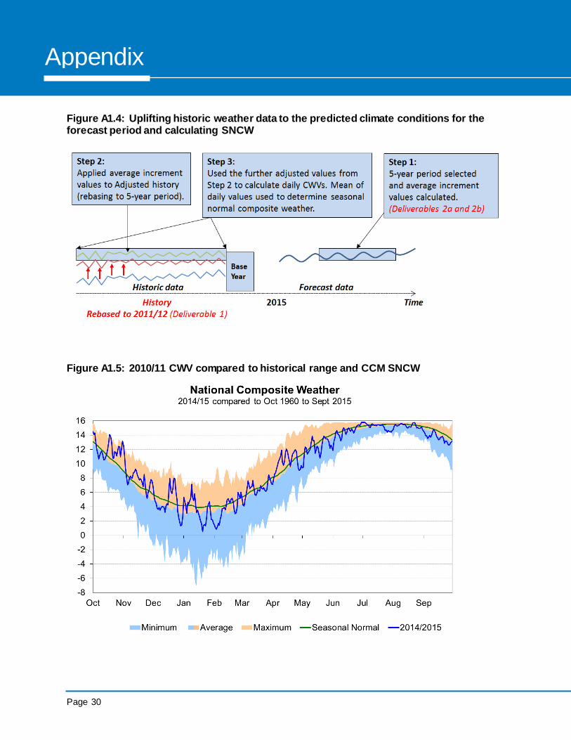
The CCM seasonal normal composite weather (SNCW) is based on historical weather adjusted for forecast warming of the UK climate. CCM refers to Climate Change Methodology9. This was the name of a project between gas industry companies and the Met Office to provide Xoserve and the demand estimation sub committee (DESC) with information needed to calculate the seasonal normal weather appropriate for the period 2015-2020. This project was split into two deliverables and was the pre-requisite for calculating a new SNCW basis. Both the Met Office deliverables and the high level steps for calculating the new SNCW basis are shown in Figure A1.4.

The first deliverable was to provide an adjusted view of historic hourly weather reflecting the estimated impacts of climate change to a known point. This “known point”, or baseline year was selected as 2011/2012. The adjusted view (represented in Figure A1.4 by the red line) was derived from the raw historic data provided via the Weather Station Substitution Methodology (WSSM) (the blue line). The WSSM historic data replaces our previous weather history and is designed to provide a consistent weather history for use in the gas industry and provided by a reputable meteorological services company. The second deliverable from the Met Office considered future changes to the climate. Based on the predicted impact of climate change trends on the future, predicted hourly seasonal normal values for the period from 1

st October 2012 to 30

th September 2025 were developed. The

difference between these values and the base year (2011/12) gave a series of hourly increment values that could be used to further adjust the base year data up to the predicted seasonal normal conditions of the future period. Revision of the basis of the seasonal normal composite weather (SNCW) followed the update of the Composite Weather Variable (CWV) definition, which as noted in A1.1, was undertaken in 2014. During this process it was decided to use a use a period of 5 years, representing 2015 to 2020, to average the increment values. These average increments were applied to the adjusted history (represented in Figure A1.4 by the red line) in order to calculate predicted hourly data that represents the average climate conditions expected in 2015-2020 (the green line). These hourly values were then converted into daily CWVs using the formula for the composite weather variable as given in A.1. Finally a SNCW value for each day in a year was calculated as the mean of the historic daily CWVs. For more info please refer to the ‘DESC Approach to derivation of new Seasonal Normal Basis’10.

9 http://www.metoffice.gov.uk/media/pdf/9/2/Xoserve_case_study-tagged.pdf

10 http://www.gasgovernance.co.uk/DESC/171214

Appendix

Figure A1.4: Uplifting historic weather data to the predicted climate conditions for the forecast period and calculating SNCW

Figure A1.5: 2010/11 CWV compared to historical range and CCM SNCW


Statement

Appendix

Appendix 2: Daily Demand Modelling A2.1 The composite weather variable greatly simplifies the structure of the weather/demand model. The consistency of CWV parameters for a number of years helps to reduce volatility in demand models from year to year. The simplicity of the demand models makes it easier to combine models for different load bands and to scale the models to annual demands.

A2.2 Load Bands

Gas consumers are grouped by load band. Load bands are categorised by the expected consumption of each gas consumer in a seasonal normal year. They are not categorised by type of customer. NDM load band models are provided as per Xoserve’s demand estimation proposals. These sample models are then scaled to the total NDM regression model. Some of the larger DM sites have demand patterns that have predictable step changes throughout the year. Individual models are calculated for these and other selected large loads, including all the sites directly connected to the NTS. These single site models are created from demand profiles and weather/demand regression models. The demand profiles are based on observed patterns in historical demand as well as information known about future demand changes. Examples include sugar beet factories that only operate at certain times of the year and the temporary closure of car factories during the recent recession. Total DM models are calculated using total DM daily demand within the LDZ, but with selected large loads removed. Total LDZ and national models are calculated by adding together the model parameters for each of the load band and individual site models.

Appendix

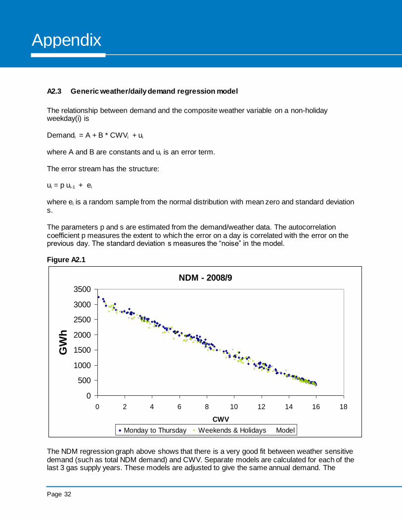
A2.3 Generic weather/daily demand regression model

The relationship between demand and the composite weather variable on a non-holiday weekday(i) is Demandi = A + B * CWVi + ui

where A and B are constants and ui is an error term. The error stream has the structure:

ui = p ui-1 + ei

where ei is a random sample from the normal distribution with mean zero and standard deviation s. The parameters p and s are estimated from the demand/weather data. The autocorrelation coefficient p measures the extent to which the error on a day is correlated with the error on the previous day. The standard deviation s measures the “noise” in the model. Figure A2.1

NDM - 2008/9

0

500

1000

1500

2000

2500

3000

3500

0 2 4 6 8 10 12 14 16 18

CWV

GW

h

Monday to Thursday Weekends & Holidays Model

The NDM regression graph above shows that there is a very good fit between weather sensitive demand (such as total NDM demand) and CWV. Separate models are calculated for each of the last 3 gas supply years. These models are adjusted to give the same annual demand. The


Statement

Appendix

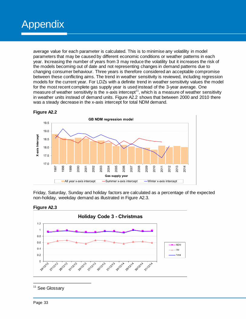
average value for each parameter is calculated. This is to minimise any volatility in model parameters that may be caused by different economic conditions or weather patterns in each year. Increasing the number of years from 3 may reduce the volatility but it increases the risk of the models becoming out of date and not representing changes in demand patterns due to changing consumer behaviour. Three years is therefore considered an acceptable compromise between these conflicting aims. The trend in weather sensitivity is reviewed, including regression models for the current year. For LDZs with a definite trend in weather sensitivity values the model for the most recent complete gas supply year is used instead of the 3-year average. One measure of weather sensitivity is the x-axis intercept11, which is a measure of weather sensitivity in weather units instead of demand units. Figure A2.2 shows that between 2000 and 2010 there was a steady decrease in the x-axis intercept for total NDM demand. Figure A2.2

Friday, Saturday, Sunday and holiday factors are calculated as a percentage of the expected non-holiday, weekday demand as illustrated in Figure A2.3. Figure A2.3

11 See Glossary

Appendix

A2.4 Conversion to daily models

The regression models are converted to daily models before adjusting for growth in demand and changes to connected load. The regression model is Demandi = A + B * CWVi + ui

This is rearranged as: Demandi = SNDi + B * (CWVi – SNCW i) + ui where SNDi is the seasonal normal demand for day i, given by: SNDi = A + B * SNCW i and SNCW i is the seasonal normal value of the CWV for day i. Weekend and holiday adjustments are incorporated into the SND and weather sensitivity (B) terms to produce a separate model for each day of the year: Demandi = SNDi + Weather Sensitivityi * (CWVi –SNCW i) + ui

A2.5 Production of forward-looking LDZ daily demand models

Each LDZ load band model is scaled separately. The first stage is to calculate the connected load for each day of the forecast. The connected load at the midpoint of each year is set equal to the forecast annual demand. Linear interpolation is then used to calculate the connected load on all the other days of the year. A profile of demand is calculated from the regression model and the seasonal normal composite weather divided by the average daily demand. Combining the profile with the forecast connected load produces the seasonal normal demand part of the daily forecast model. The weather sensitivity term is scaled by connected load forecast divided by regression model average daily demand. Changes in connected load, due to step changes in large load demand, are excluded from the generic DM load bands. These large loads are treated as separate individual load bands. Total DM load band models are created by adding the generic DM load band models to the individual large load models. A total NDM model is created from the sum of the NDM load band models, and total LDZ from the sum of total NDM and DM models plus shrinkage. The profile of each model is validated against historical data.


Statement

Appendix

A2.6 NTS and selected DM site daily demand models

Demand models are created for every load connected to the NTS and for a small number of LDZ large loads. These models consist of a regression model with the same parameters and calculated in the same way as the LDZ models plus a profile adjustment. The profile adjustment consists of a date from which the profile changes and a multiplier to adjust the profile. This enables unique site profiles, for example sugar beet factories, and demand response reductions to be accommodated. Generic models are created for new sites. These models are scaled to the forecast connected load and then converted to daily models with a seasonal normal and weather sensitivity term using similar methodology to the LDZ forecasts.

Profile adjustments are manual estimates based on historical observations. An initial estimate is made. Forecasts are produced for the base year and compared with actual demand. This ensures that when annual, regression and profile elements of the forecast are combined the desired results are achieved. If necessary adjustments are made to the profiles and the process repeated.

A2.7 National demand models

The LDZ modelling process is repeated to produce a national LDZ demand model calculated from the total LDZ demand and the national CWV. The forecast daily demand models derived from this process are added to the NTS site daily demand models to produce a National daily demand model. The peaks and load duration curves derived directly from the national models are different from those calculated by adding up the individual LDZ and NTS peak and load duration curve forecasts. Load curves produced from national demand models are known as diversified load duration curves. Those produced by adding up the LDZ and NTS values are known as undiversified.

Appendix

Appendix 3 Load Duration Curve Production12

A3.1 Process of demand simulation

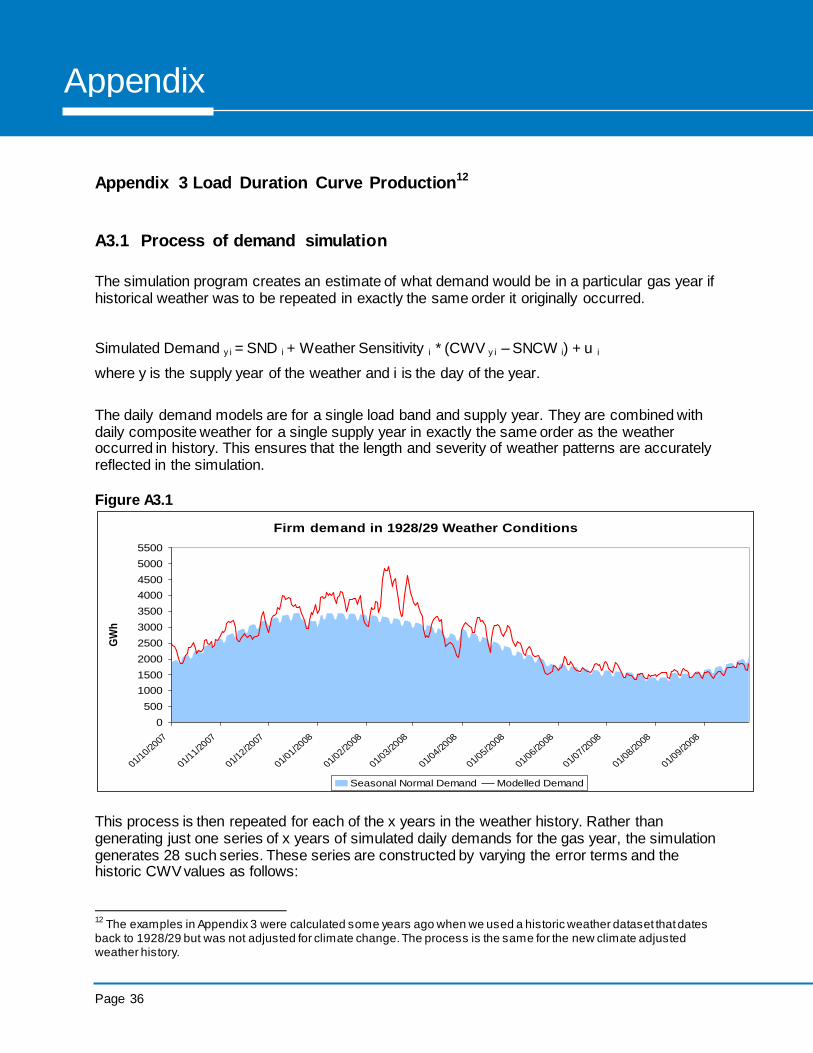
The simulation program creates an estimate of what demand would be in a particular gas year if historical weather was to be repeated in exactly the same order it originally occurred.

Simulated Demand y i = SND i + Weather Sensitivity i * (CWV y i – SNCW i) + u i

where y is the supply year of the weather and i is the day of the year.

The daily demand models are for a single load band and supply year. They are combined with daily composite weather for a single supply year in exactly the same order as the weather occurred in history. This ensures that the length and severity of weather patterns are accurately reflected in the simulation.

Figure A3.1

Firm demand in 1928/29 Weather Conditions

0

500

1000

1500

2000

2500

3000

3500

4000

4500

5000

5500

01/10/2

007

01/11/2

007

01/12/2

007

01/01/2

008

01/02/2

008

01/03/2

008

01/04/2

008

01/05/2

008

01/06/2

008

01/07/2

008

01/08/2

008

01/09/2

008

GW

h

Seasonal Normal Demand Modelled Demand

This process is then repeated for each of the x years in the weather history. Rather than generating just one series of x years of simulated daily demands for the gas year, the simulation generates 28 such series. These series are constructed by varying the error terms and the historic CWV values as follows:

12

The examples in Appendix 3 were calculated some years ago when we used a historic weather dataset that dates back to 1928/29 but was not adjusted for climate change. The process is the same for the new climate adjusted weather history.


Statement

Appendix

Seven different simulations are generated, by shifting the historic CWV values forwards by one, two and three days, and similarly backwards, in addition to the base run. This ensures that the extreme CWV values occur on every individual day of the week in the overall simulation.

For each positioning of the historic CWV values two independent sets of random error terms are generated, and for each of these sets a corresponding antithetic error stream is generated as follows:

random error, u i = p u i-1 + e i

antithetic random error, u* i = p * u* i-1 – e i

The use of antithetic random error terms is a variance reduction technique, which minimises the chance of bias in the overall set of results.

This approach therefore yields 7*2*2 = 28 sets of simulated demands, each comprising x gas years.

A3.2 Calculation of the 1 in 20 peak day

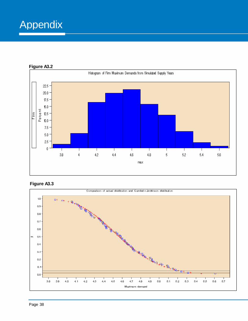
For each of the 28 simulations there are x maximum daily, simulated demands (one for each gas year in the historic weather database). A Gumbel-Jenkinson distribution is fitted to these x values. This distribution is designed for fitting to extreme events and is often used in analysis of extreme weather. Similar results can be obtained by using a Weibull distribution. A 1 in 20 peak day value is calculated for each of the 28 sets of simulations from the 95 percent value from the distribution. The 28 1 in 20 peak day estimates are averaged to give the 1 in 20 peak day. Note that only the maximum daily demand in each simulated year is considered. Thus in a very cold winter when the 1 in 20 peak demand is exceeded, there may be more than one day when demand exceeds the 1 in 20 value. The following two graphs are derived from all the years in one set of simulations of firm demand. Figure A3.2 shows the shape of the distribution of the maximum demands for each year. Figure A3.3 shows the cumulative distribution for this data (blue) compared with the fitted Gumbel-Jenkinson distribution (red). The Y-axis shows the probability of maximum demand exceeding the value on the X-axis. The horizontal lines are the 1 in 20 peak day and the 1 in 50 level, which becomes day 1 on the 1 in 50 load duration curve.

Appendix

Figure A3.2

Figure A3.3


Statement

Appendix

A3.3 Calculation of the Average Peak Day

The average peak day demand is the mean of the maximum daily demands in each simulated year, described in section A3.1. It is the average highest demand day in a year.

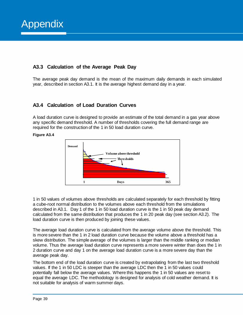
A3.4 Calculation of Load Duration Curves

A load duration curve is designed to provide an estimate of the total demand in a gas year above any specific demand threshold. A number of thresholds covering the full demand range are required for the construction of the 1 in 50 load duration curve.

Figure A3.4

1 in 50 values of volumes above thresholds are calculated separately for each threshold by fitting a cube-root normal distribution to the volumes above each threshold from the simulations described in A3.1. Day 1 of the 1 in 50 load duration curve is the 1 in 50 peak day demand calculated from the same distribution that produces the 1 in 20 peak day (see section A3.2). The load duration curve is then produced by joining these values.

The average load duration curve is calculated from the average volume above the threshold. This is more severe than the 1 in 2 load duration curve because the volume above a threshold has a skew distribution. The simple average of the volumes is larger than the middle ranking or median volume. Thus the average load duration curve represents a more severe winter than does the 1 in 2 duration curve and day 1 on the average load duration curve is a more severe day than the average peak day.

The bottom end of the load duration curve is created by extrapolating from the last two threshold values. If the 1 in 50 LDC is steeper than the average LDC then the 1 in 50 values could potentially fall below the average values. Where this happens the 1 in 50 values are reset to equal the average LDC. The methodology is designed for analysis of cold weather demand. It is not suitable for analysis of warm summer days.

Volume above threshold Thresholds

Days 365 1

Demand

Appendix

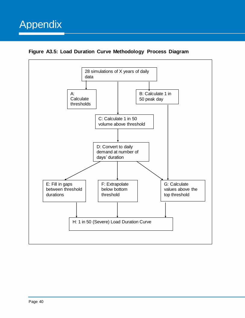
Figure A3.5: Load Duration Curve Methodology Process Diagram

28 simulations of X years of daily data

A: Calculate thresholds

C: Calculate 1 in 50

volume above threshold

B: Calculate 1 in

50 peak day

D: Convert to daily demand at number of

days’ duration

E: Fill in gaps between threshold

durations

F: Extrapolate below bottom

threshold

G: Calculate values above the

top threshold

H: 1 in 50 (Severe) Load Duration Curve


Statement

Appendix

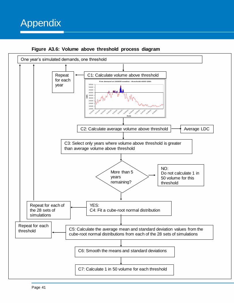
Figure A3.6: Volume above threshold process diagram

One year’s simulated demands, one threshold

C1: Calculate volume above threshold

C2: Calculate average volume above threshold

C3: Select only years where volume above threshold is greater

than average volume above threshold

More than 5 years

remaining?

NO: Do not calculate 1 in 50 volume for this threshold

YES: C4: Fit a cube-root normal distribution

C5: Calculate the average mean and standard deviation values from the cube-root normal distributions from each of the 28 sets of simulations

Repeat for each of the 28 sets of simulations

Repeat for each

threshold

C6: Smooth the means and standard deviations

C7: Calculate 1 in 50 volume for each threshold

Firm demand at 1928/29 weather - threshold=4000 GWh

1000

1500

2000

2500

3000

3500

4000

4500

5000

5500

01 /10 /0

4

01 /11 /0

4

01 /12 /0

4

01 /01 /0

5

01 /02 /0

5

01 /03 /0

5

01 /04 /0

5

01 /05 /0

5

01 /06 /0

5

01 /07 /0

5

01 /08 /0

5

01 /09 /0

5

Date

GW

h

Repeat for each year

Average LDC

Appendix

Step A: Calculate thresholds

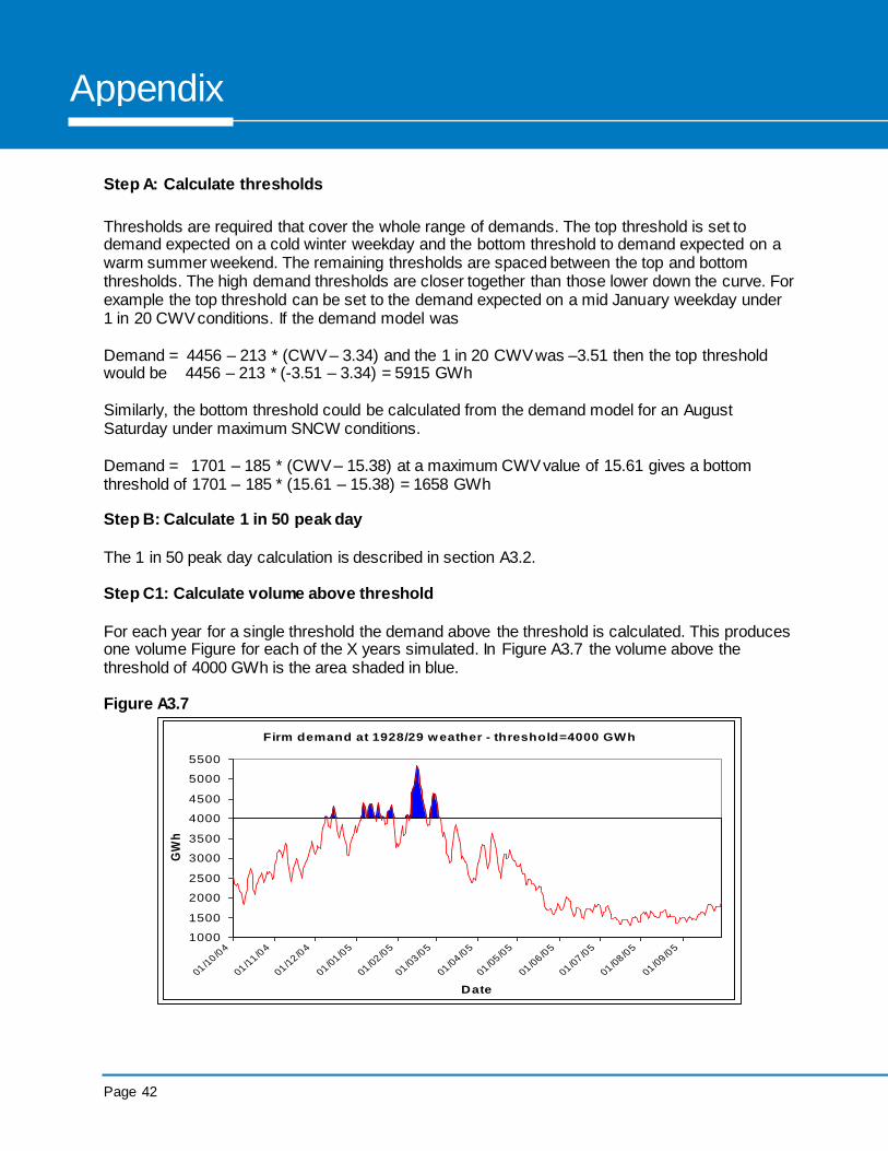
Thresholds are required that cover the whole range of demands. The top threshold is set to demand expected on a cold winter weekday and the bottom threshold to demand expected on a warm summer weekend. The remaining thresholds are spaced between the top and bottom thresholds. The high demand thresholds are closer together than those lower down the curve. For example the top threshold can be set to the demand expected on a mid January weekday under 1 in 20 CWV conditions. If the demand model was Demand = 4456 – 213 * (CWV – 3.34) and the 1 in 20 CWV was –3.51 then the top threshold would be 4456 – 213 * (-3.51 – 3.34) = 5915 GWh Similarly, the bottom threshold could be calculated from the demand model for an August Saturday under maximum SNCW conditions. Demand = 1701 – 185 * (CWV – 15.38) at a maximum CWV value of 15.61 gives a bottom threshold of 1701 – 185 * (15.61 – 15.38) = 1658 GWh Step B: Calculate 1 in 50 peak day

The 1 in 50 peak day calculation is described in section A3.2. Step C1: Calculate volume above threshold

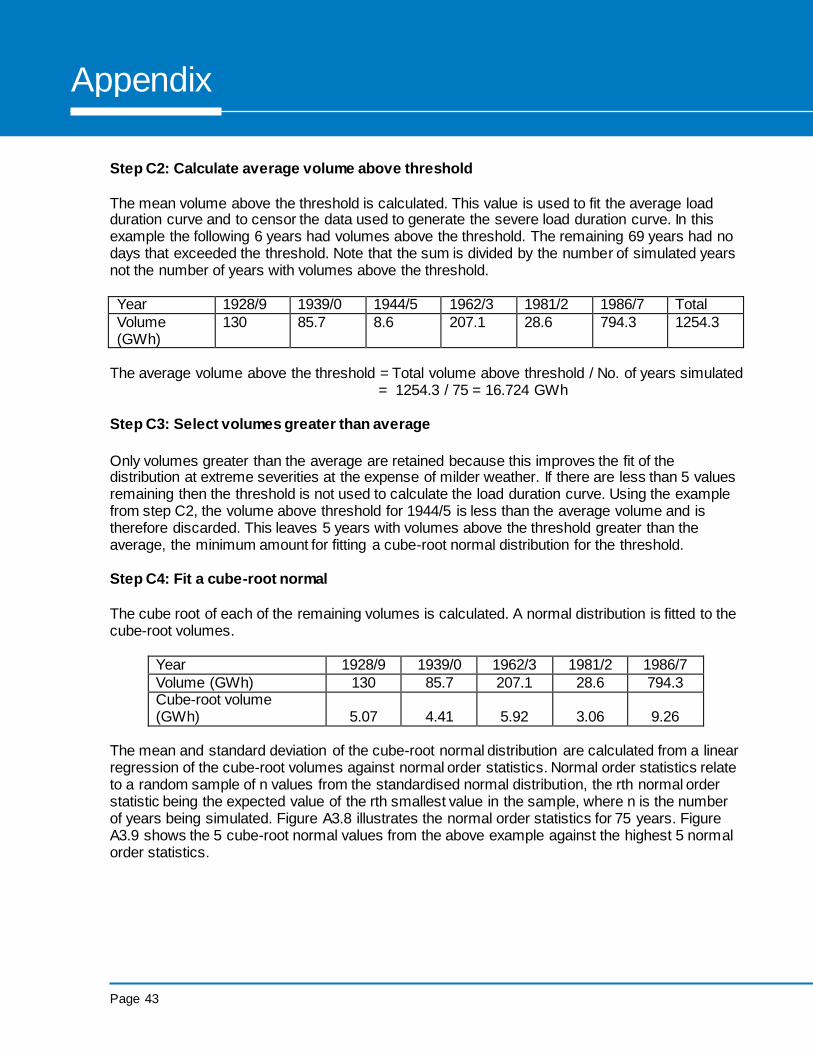
For each year for a single threshold the demand above the threshold is calculated. This produces one volume Figure for each of the X years simulated. In Figure A3.7 the volume above the threshold of 4000 GWh is the area shaded in blue. Figure A3.7

Firm demand at 1928/29 weather - threshold=4000 GWh

1000

1500

2000

2500

3000

3500

4000

4500

5000

5500

01 /10 /0

4

01 /11 /0

4

01 /12 /0

4

01 /01 /0

5

01 /02 /0

5

01 /03 /0

5

01 /04 /0

5

01 /05 /0

5

01 /06 /0

5

01 /07 /0

5

01 /08 /0

5

01 /09 /0

5

Date

GW

h


Statement

Appendix

Step C2: Calculate average volume above threshold

The mean volume above the threshold is calculated. This value is used to fit the average load duration curve and to censor the data used to generate the severe load duration curve. In this example the following 6 years had volumes above the threshold. The remaining 69 years had no days that exceeded the threshold. Note that the sum is divided by the number of simulated years not the number of years with volumes above the threshold. Year 1928/9 1939/0 1944/5 1962/3 1981/2 1986/7 Total

Volume (GWh)

130 85.7 8.6 207.1 28.6 794.3 1254.3

The average volume above the threshold = Total volume above threshold / No. of years simulated = 1254.3 / 75 = 16.724 GWh

Step C3: Select volumes greater than average

Only volumes greater than the average are retained because this improves the fit of the distribution at extreme severities at the expense of milder weather. If there are less than 5 values remaining then the threshold is not used to calculate the load duration curve. Using the example from step C2, the volume above threshold for 1944/5 is less than the average volume and is therefore discarded. This leaves 5 years with volumes above the threshold greater than the average, the minimum amount for fitting a cube-root normal distribution for the threshold.

Step C4: Fit a cube-root normal

The cube root of each of the remaining volumes is calculated. A normal distribution is fitted to the cube-root volumes.

Year 1928/9 1939/0 1962/3 1981/2 1986/7

Volume (GWh) 130 85.7 207.1 28.6 794.3 Cube-root volume (GWh) 5.07 4.41 5.92 3.06 9.26

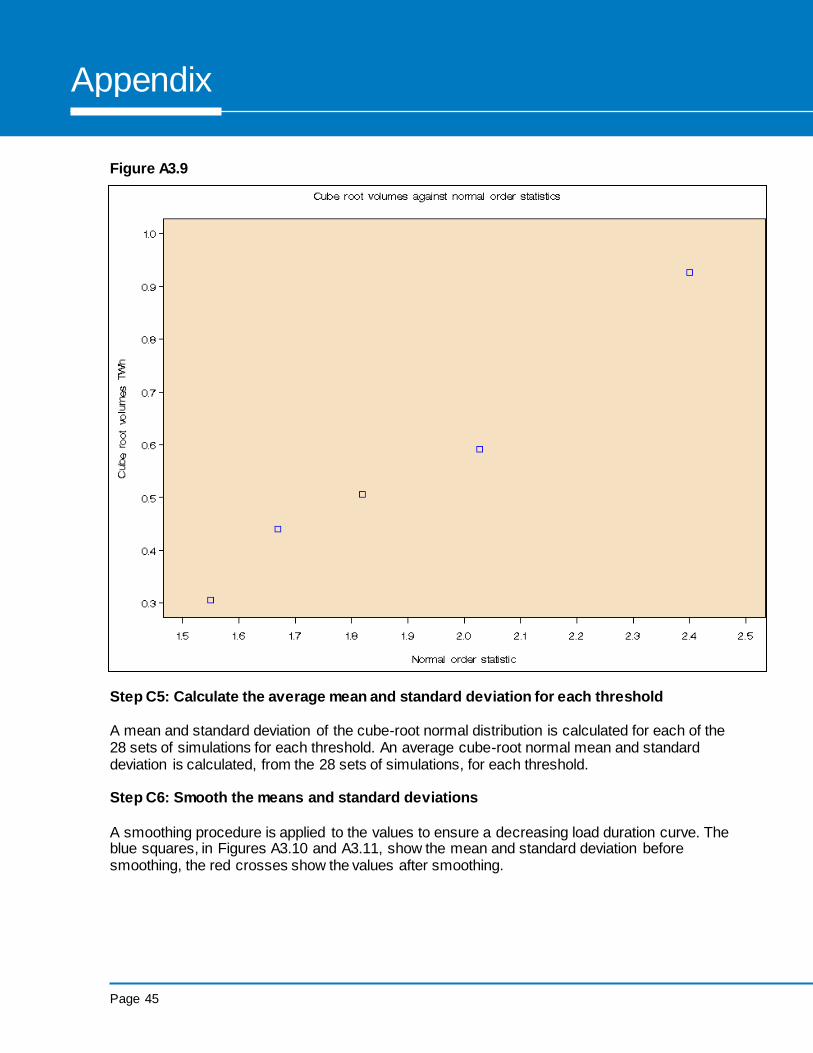
The mean and standard deviation of the cube-root normal distribution are calculated from a linear regression of the cube-root volumes against normal order statistics. Normal order statistics relate to a random sample of n values from the standardised normal distribution, the rth normal order statistic being the expected value of the rth smallest value in the sample, where n is the number of years being simulated. Figure A3.8 illustrates the normal order statistics for 75 years. Figure A3.9 shows the 5 cube-root normal values from the above example against the highest 5 normal order statistics.

Appendix

Figure A3.8

The five normal order statistics used in

the regression illustrated in Figure A3.9

Normal order statistics against number of years


Statement

Appendix

Figure A3.9

Step C5: Calculate the average mean and standard deviation for each threshold

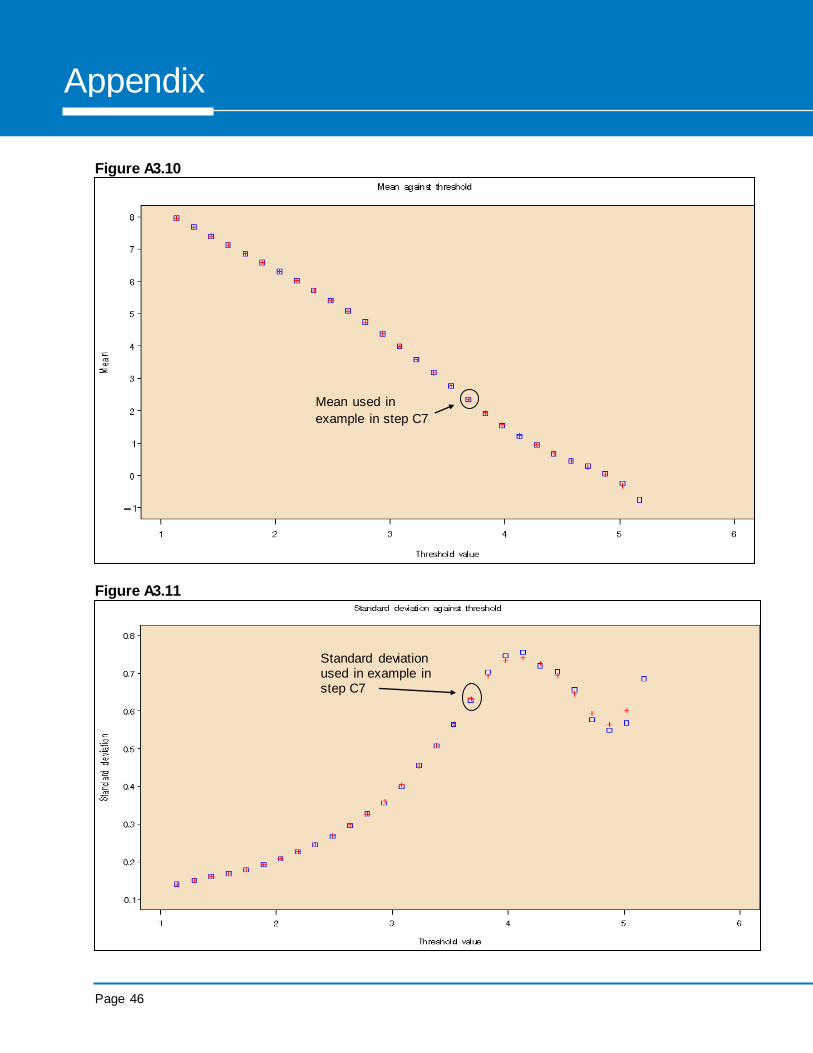
A mean and standard deviation of the cube-root normal distribution is calculated for each of the 28 sets of simulations for each threshold. An average cube-root normal mean and standard deviation is calculated, from the 28 sets of simulations, for each threshold. Step C6: Smooth the means and standard deviations

A smoothing procedure is applied to the values to ensure a decreasing load duration curve. The blue squares, in Figures A3.10 and A3.11, show the mean and standard deviation before smoothing, the red crosses show the values after smoothing.

Appendix

Figure A3.10

Figure A3.11

Standard deviation used in example in step C7

Mean used in

example in step C7


Statement

Appendix

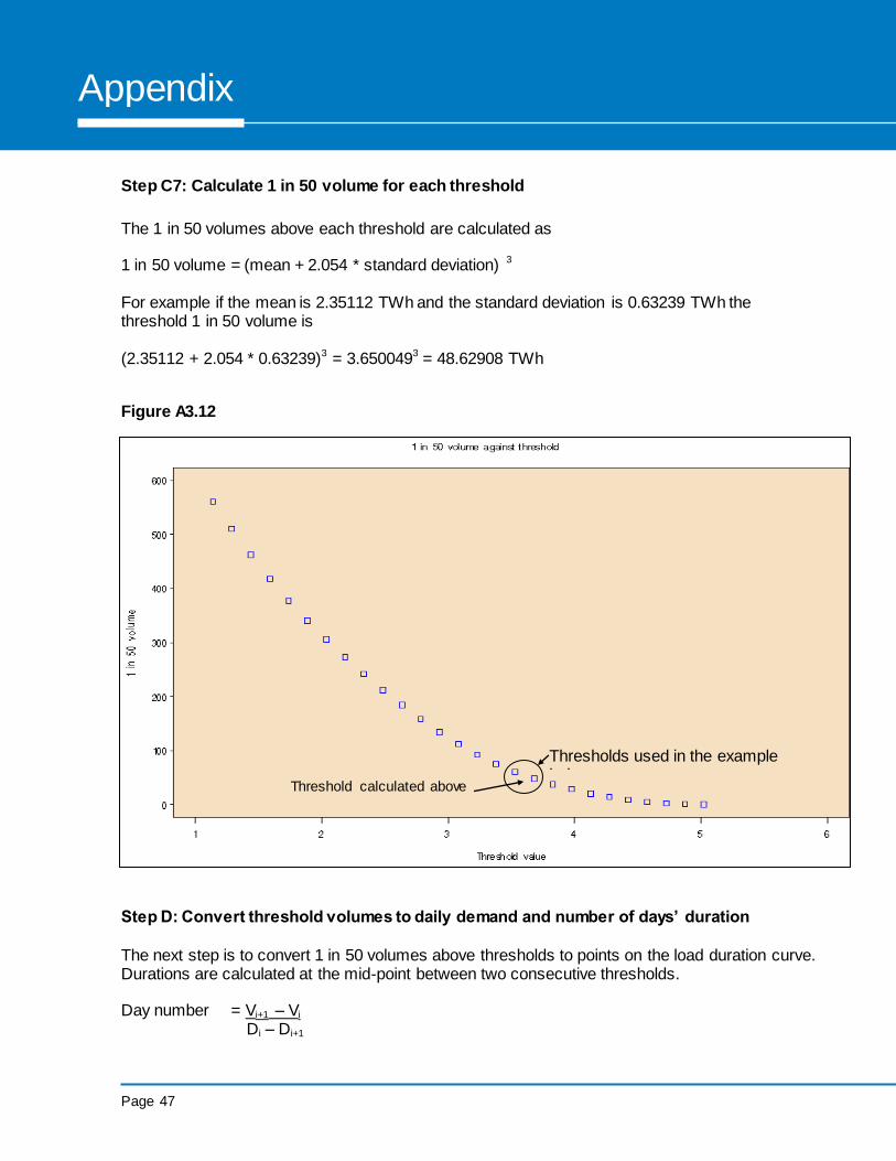
Step C7: Calculate 1 in 50 volume for each threshold

The 1 in 50 volumes above each threshold are calculated as 1 in 50 volume = (mean + 2.054 * standard deviation) 3 For example if the mean is 2.35112 TWh and the standard deviation is 0.63239 TWh the threshold 1 in 50 volume is (2.35112 + 2.054 * 0.63239)3 = 3.6500493 = 48.62908 TWh

Figure A3.12

Step D: Convert threshold volumes to daily demand and number of days’ duration

The next step is to convert 1 in 50 volumes above thresholds to points on the load duration curve. Durations are calculated at the mid-point between two consecutive thresholds. Day number = Vi+1 – Vi Di – Di+1

Thresholds used in the example below

Threshold calculated above

Appendix

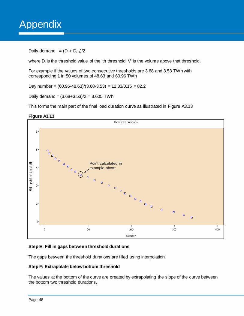
Daily demand = (Di + Di+1)/2 where Di is the threshold value of the ith threshold, Vi is the volume above that threshold. For example if the values of two consecutive thresholds are 3.68 and 3.53 TWh with corresponding 1 in 50 volumes of 48.63 and 60.96 TWh Day number = (60.96-48.63)/(3.68-3.53) = 12.33/0.15 = 82.2 Daily demand = (3.68+3.53)/2 = 3.605 TWh This forms the main part of the final load duration curve as illustrated in Figure A3.13 Figure A3.13

Step E: Fill in gaps between threshold durations

The gaps between the threshold durations are filled using interpolation. Step F: Extrapolate below bottom threshold

The values at the bottom of the curve are created by extrapolating the slope of the curve between the bottom two threshold durations.

Point calculated in example above


Statement

Appendix

Step G: Calculate values above the top threshold

The gap between day 1 and the highest threshold is filled by fitting a cubic equation that satisfies the following constraints:

i) Day 1 is set to the 1 in 50 peak day demand. ii) The demand from the cubic equation must equal the demand from the volume analysis where the two curves meet. iii) The area under the fitted curve and above the demand threshold corresponding to the point where the two curves meet must be equal to the 1 in 50 volume derived from the volume analysis for this threshold. iv) The slopes of the two curves should be the same where the two curves meet.

Step H: Combine to produce the 1 in 50 load duration curve

Figure A3.14 shows the final 1 in 50 load duration curve in red with blue squares showing the cube-root normal values. Figure A3.14

Appendix

Appendix 4: Extract from the Gas Transporters Licence

Standard Special Condition A9. Pipe-Line System Security Standards

1. The licensee shall, subject to section 9 of the Act, plan and develop its pipe-line system so as to enable it to meet, having regard to its expectations as to – (a) the number of premises to which gas conveyed by it will be supplied; (c) the consumption of gas at those premises; and (c) the extent to which the supply of gas to those premises might be interrupted or reduced (otherwise than in pursuance of such a term as is mentioned in paragraph 3 of standard condition 14 (Security and emergency arrangements) of the standard conditions of gas suppliers’ licences or of directions given under section 2(1)(b) of the Energy Act 1976) in pursuance of contracts between any of the following persons, namely, a gas transporter, a gas shipper, a gas supplier and a customer of a gas supplier, the gas security standard mentioned in paragraph 2. 2. The gas security standard referred to in paragraph 1 is that the pipe-line system to which this licence relates (taking account of such operational measures as are available to the licensee including, in particular, the making available of stored gas) meets the peak aggregate daily demand, including, but not limited to, within day gas flow variations on that day, for the conveyance of gas for supply to premises which the licensee expects to be supplied with gas conveyed by it – (a) which might reasonably be expected if the supply of gas to such premises were interrupted or reduced as mentioned in paragraph 1(c); and (b) which, (subject as hereinafter provided) having regard to historical weather data derived from at least the previous 50 years and other relevant factors, is likely to be exceeded (whether on one or more days) only in 1 year out of 20 years, so, however, that if, after consultation with all gas suppliers, gas shippers and gas transporters, with the Health and Safety Executive and with the Consumer Council, the Authority is satisfied that security standards would be adequate if sub-paragraph (b) were modified by the substitution of a reference to data derived from a period of less than the previous 50 years or by the substitution of some higher probability for the probability of 1 year in 20 years, the Authority may, subject to paragraph 3, make such modifications by a notice which – (i) is given and published by the Authority for the purposes of this condition generally; and (ii) specifies the modifications and the date on which they are to take effect. 3. Paragraph 2(b) shall only be modified if, at the same time, the Authority makes similar modifications to (a) paragraph 6(b) of standard condition 14 (Security and Emergency Arrangements) and paragraph 5(a) of standard condition 32A (Security of Supply – Domestic Customers) of the standard conditions of gas suppliers’ licences; and (b) sub-paragraph (b) of the definition of “security standards” in standard condition 1 (Definitions and Interpretation) of the standard conditions of gas shippers’ licences.


Statement

Appendix

4. For the purposes of paragraph 1, the licensee may have regard to information received from the operator of a pipe-line or pipe-line system to which it conveys gas as respects the quantity of gas which it expects to require.

Appendix 5: References A copy of Jenkinson’s revisions to the Gumbel distribution is held at the Modern Records Centre at the University of Warwick reference MSS.335/GA/4/14/15. The title of the paper is “The frequency distribution of the annual maximum (or minimum) values of meteorological elements” by A.F.Jenkinson, Meteorological Office, London. The offtake arrangements document section H – NTS long term demand forecasting is available from the Joint Office of Gas Transporters website. http://www.gasgovernance.co.uk/OAD Government energy statistics can be obtained from https://www.gov.uk/government/organisations/department-for-business-energy-and-industrial-strategy/about/statistics

http://www.gasgovernance.co.uk/OAD

https://www.gov.uk/government/organisations/department-for-business-energy-and-industrial-strategy/about/statistics

https://www.gov.uk/government/organisations/department-for-business-energy-and-industrial-strategy/about/statistics

Appendix

Appendix 6: Data in the public domain Selected Figures from the demand forecasts can be obtained from the National Grid website. Ten Year Statement

The ten year statement is the main document containing demand and supply forecasts. It is published every December. As well as the TYS document a spreadsheet is provided with the data behind the charts and tables. Annual and peak day forecasts and selected load duration curves are available. http://www.nationalgrid.com/gtys Demand and weather profiles

Seasonal normal cold and warm composite weather and daily demand at seasonal normal cold and warm weather conditions. http://www.nationalgrid.com/uk/Gas/Data/misc/ Gas demand data and composite weather variables can be downloaded from the National Grid web site. http://marketinformation.natgrid.co.uk/gas/DataItemExplorer.aspx Future Energy Scenarios

This document describes the assumptions behind the main forecasting scenarios. This is the first publication of the demand and supply forecasts which feed into the Ten Year Statement. http://www.nationalgrid.com/fes Met Office Climate Change Methodology project

Information about the CCM project and climate forecasts can be found on the Met Office web site. http://www.metoffice.gov.uk/media/pdf/9/2/Xoserve_case_study-tagged.pdf Gas Transporter’s Licence

https://www.ofgem.gov.uk/licences-codes-and-standards/licences/licence-conditions

http://www.nationalgrid.com/gtys

http://www.nationalgrid.com/uk/Gas/Data/misc/

http://marketinformation.natgrid.co.uk/gas/DataItemExplorer.aspx

http://www.nationalgrid.com/fes

http://www.metoffice.gov.uk/media/pdf/9/2/Xoserve_case_study-tagged.pdf

https://www.ofgem.gov.uk/licences-codes-and-standards/licences/licence-conditions


Statement

Appendix

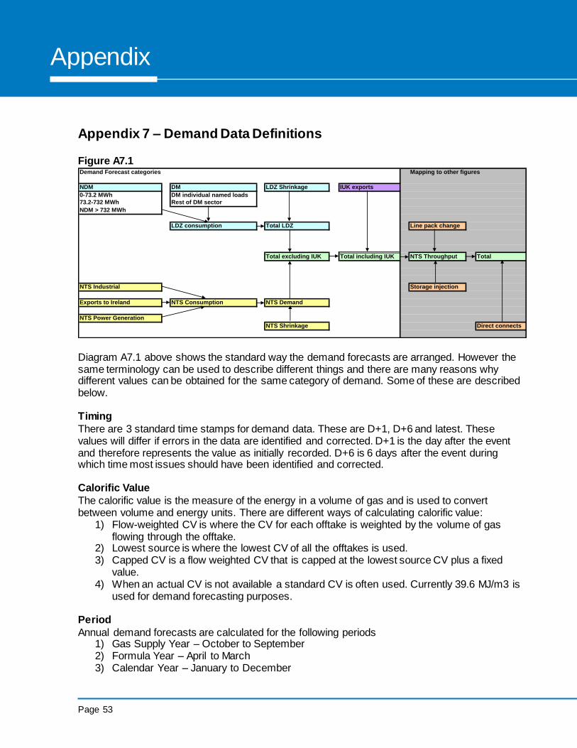
Appendix 7 – Demand Data Definitions Figure A7.1 Demand Forecast categories Mapping to other figures

NDM DM LDZ Shrinkage IUK exports

0-73.2 MWh DM individual named loads

73.2-732 MWh Rest of DM sector

NDM > 732 MWh

LDZ consumption Total LDZ Line pack change

Total excluding IUK Total including IUK NTS Throughput Total

NTS Industrial Storage injection

Exports to Ireland NTS Consumption NTS Demand

NTS Power Generation

NTS Shrinkage Direct connects

Diagram A7.1 above shows the standard way the demand forecasts are arranged. However the same terminology can be used to describe different things and there are many reasons why different values can be obtained for the same category of demand. Some of these are described below. Timing

There are 3 standard time stamps for demand data. These are D+1, D+6 and latest. These values will differ if errors in the data are identified and corrected. D+1 is the day after the event and therefore represents the value as initially recorded. D+6 is 6 days after the event during which time most issues should have been identified and corrected. Calorific Value

The calorific value is the measure of the energy in a volume of gas and is used to convert between volume and energy units. There are different ways of calculating calorific value:

1) Flow-weighted CV is where the CV for each offtake is weighted by the volume of gas flowing through the offtake.

2) Lowest source is where the lowest CV of all the offtakes is used. 3) Capped CV is a flow weighted CV that is capped at the lowest source CV plus a fixed

value. 4) When an actual CV is not available a standard CV is often used. Currently 39.6 MJ/m3 is

used for demand forecasting purposes. Period

Annual demand forecasts are calculated for the following periods 1) Gas Supply Year – October to September 2) Formula Year – April to March 3) Calendar Year – January to December

Appendix

Weather basis

Variability in non-daily metered (NDM) demand is mainly due to the weather. Demand values are often adjusted to the same weather basis to make it easier to compare different values. These include

1) Actual weather 2) Long term historical average. National Grid’s weather data base starts in 1960. 3) CCM seasonal normal. A climate adjusted and smoothed seasonal normal weather profile 4) Energy Phase 2 (EP2) seasonal normal. This was the seasonal normal basis used prior to

CCM. The name refers to a project between energy companies and the Met Office to look at the implications of climate change on the energy industry.

Line pack

The gas contained in NTS network is called line pack. This changes from day to day depending on the pressure. Total demands can be calculated both including and excluding line pack. Storage injection

Injection into gas storage can be included or excluded from total demand. Stock change

Stock change is the combination of changes to line pack and changes to storage levels Direct connects

Some large users take some of their gas directly from gas fields without the gas passing through the National Transmission System. National Grid Figures normally exclude these supplies whist Department for Business, Energy and Industrial Strategy (BEIS) Figures include them. Physical/deemed

The total of all commercial exports through the IUK are called deemed exports. These are normally higher than the physical flows through the IUK. Physical exports = (Deemed exports – deemed imports) For most purposes physical is more appropriate but for financial purposes deemed tends to be used. CHP

Combined heat and power sites can sometimes be categorised as industrial loads and sometimes as power generators. Electricity definition power generation In documents, such as the Winter Outlook report, where both electricity and gas are discussed gas power generation demand is often defined to match that used for electricity generation. This takes all the NTS power generation loads, adds some large CHP loads from the industrial list and the large power stations in the LDZs that are connected to the electricity transmission network.


Statement

Glossary

1 in 20 Peak Day: 1 in 20 peak day demand is the level of daily demand that, in a long series of winters, with connected load held at the levels appropriate to the winter in question, would be exceeded in one out of 20 winters, with each winter counted only once.

1 in 50 Load Duration Curve: The 1 in 50 load duration curve is that curve which, in a long series of years, with connected load held at the levels appropriate to the year in question, would be such that the

volume of demand above any given demand threshold (represented by the area under the curve and above the threshold) would be exceeded in one out of 50 years. It is also called the severe year curve.

Actual Temperature: Thermometer readings. Daily temperature is the weighted average of 12 2-hourly temperatures over the gas day.

Calorific value (CV): The amount of energy, in megajoules, released when a cubic metre of gas is completely combusted under specified conditions. Units are MJ/m3. Demand forecasts are produced in energy units and converted to volume using the following formula:

Volume (mcm) = Energy (GWh) * 3.6 / Calorific Value

If the actual CV is not available then a good approximation for national gas demand is 39.6 MJ/m3. This makes the equation very simple:

Volume (mcm) = Energy (GWh) / 11 CHP (Combined heat and power): CHP sites are power generators where the heat from the generation is

used as well as the electricity. These sites can sometimes be categorised as industrial and sometimes as power generation.

Cold and Warm profiles: Smoothed 1 in 20 cold and warm weather calculated from moving 7-day periods. Cold and warm demand profiles are calculated from the demand models and the cold and warm weather.

Composite Weather Variable (CWV): A weather variable that is linearly related to non-daily metered gas demand.

Connected Load: Connected load refers to the demand that a site, or group of sites, connected to the gas network would be expected to consume in a seasonal normal year. This is best explained with the aid of an example. Consider a large flat load that started to operate, at full capacity, on September 1st 2010. The

seasonal normal demand for the load is 3650 GWh. The seasonal normal annual demand forecast for the 2010 calendar year would be 3650GWh*122days/365days=1220. However, the connected load for all the days from January 2010 to August 31st would be zero GWh. The connected load for September 1st 2010

onwards would be 3650 GWh. Demand models are scaled to connected load forecasts, not annual demand.

Daily Metered (DM) Demand: The total amount of gas used by the higher demand customers connected to the LDZ whose meters are read daily.

Degree Days: Degree-days show the number of degrees that the daily temperature is below a specified threshold.

Degree-days = maximum (threshold temperature – daily temperature, 0). Degree days can be calculated using either CWV or temperature. The threshold is set depending on the

analysis required. A typical threshold for analysis of trends in weather is 20 degrees. For severe weather

Glossary

analysis a threshold of zero degrees is often used. Alternatively the threshold can be set to the point at which a weather demand regression line crosses the weather axis, the X-axis intercept.

Diversified Peak Day Demand: The diversified total peak day demand forecast is the national gas demand, assuming no interruption, expected in 1 in 20 cold weather conditions. Diversified peak day is used where location is not important.

DN Offtake: A point on the NTS where gas is transferred from a transmission network to a distribution network.

Effective Temperature: The effective temperature is an exponentially smoothed daily temperature.

Today’s effective temperature = 0.5 * today’s daily temperature + 0.5 * yesterday’s effective temperature CCM Seasonal Normal Weather: a climate change adjusted seasonal normal composite weather where

the climate adjustments are from the CCM project. This was a joint project between the Met Office and the UK gas industry.

Firm (Exit) Capacity: a customer’s right to take gas from the NTS (up to purchased capacity level). Gas Day: The standard time period for gas demand is a gas day. This is because gas travels at 25mph

through the National Transmission System (NTS). Gas landed in Scotland would take 23 hours to travel to the furthest point on the network in Cornwall. The gas day starts and ends at 5am when gas demand tends to be lowest.

Gas Supply Year: October to September. Typically any changes to formulae such as CWV are applied at the start of a gas year.

Interconnector exports: gas which is sent to Europe from the UK. Often just refers to exports through the IUK interconnector and not exports through the Moffat interconnector to Ireland.

Line pack: gas stored in gas pipelines. Changes in line pack are accommodated through changes in

pressure. Local Distribution Network (LDZ): The lower pressure gas pipelines which transport gas from the NTS to

final consumers.

National Transmission System: The high pressure pipelines which carries large amounts of gas around

the country Non Daily Metered (NDM) Demand: The total amount of gas used by all residential properties, most

commercial and some industrial premises within an LDZ NTS Demand: In this document NTS demand refers to the total demand for all industrial and power station

loads directly connected to the NTS transmission system plus Moffat exports plus NTS shrinkage. It excludes LDZ demand, IUK exports, and storage injection. Note that in some publications NTS demand refers to total GB demand.

Obligated Demand: The higher of sold or baseline capacity.


Statement

Glossary

Pseudo Seasonal Normal Temperature: Seasonal normal temperature adjusted to better reflect the pattern of gas demand throughout the year.

Seasonal Normal Composite Weather (SNCW, SNCWV): Composite weather expected on average each day. It is updated every few years to include the most recent years’ data and to include climate change.

Shrinkage: The difference between the amount of gas put into the network and the amount metered as used. Reasons for shrinkage include theft, leakage and compressor usage.

Storage injection: the process of taking gas off the NTS to put away into storage sites, to be released at a later time.

Therm: an imperial unit of heat energy. One therm is equal to 29.3071 kWh. Undiversified peak day demand: The peak day at every location added together. Undiversified demand is

used where location is important such as network models. X-axis intercept: A simple metric to compare the weather sensitivity of different demand models in

weather units. It is the weather value from a weather/demand regression model at a demand value of zero. A highly weather sensitive model has a steep slope, and hence a low x -axis intercept value.

Contact Details

If you have any questions please contact:

Neil Rowley Gas Modelling Manager

SO Strategy National Grid House

Gallows Hill Warwick CV34 6DA E-mail: [email protected]

mailto:[email protected]

Glossary

chapter three continued annual demand - national grid plc

Documents