chapters 1&2 - investments, investment markets, and ...zz1802/finance...
TRANSCRIPT
Chapter 1 - Investments: Background and Issues
Investment vs. investments Real assets vs. financial assets Financial markets and the economy Investment process Competitive markets Players in investment markets Recent trends Investments as a profession
Investment vs. investmentsInvestment: the commitment of current resources in the expectation of deriving greater resources in the future
For example: You cut current consumption to purchase stocks and anticipate that stock prices will rise in the futureYou forgo current leisure and income to take the investments class and expect that a degree from CSUN will enhance your future career
InvestmentsThe detailed study of the investment process - focus of this class
Real assets vs. financial assetsReal assets: assets used to produce goods and servicesFinancial assets: claims on real assets or income generated by real assets
Financial assets Fixed-income securities: paying a fixed stream of income over a specified period -CDs, bonds, T-bills, etcEquity: ownership in a corporation - stocksDerivative securities: their payoffs depend on the values of other assets - futures, options, swaps, etc (FIN 436 - Futures and Options for more details)
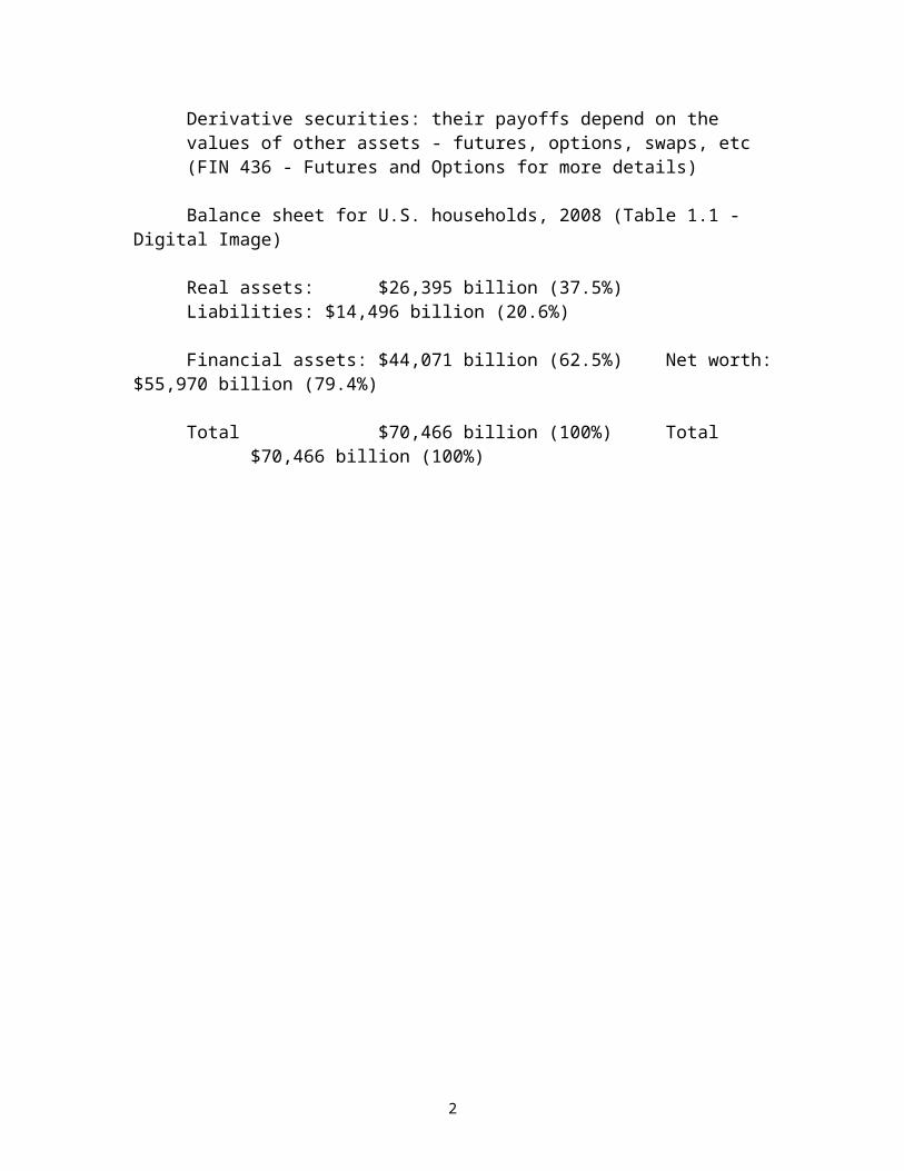
Balance sheet for U.S. households, 2008 (Table 1.1 - Digital Image)
Real assets: $26,395 billion (37.5%) Liabilities: $14,496 billion (20.6%)
Financial assets: $44,071 billion (62.5%) Net worth: $55,970 billion (79.4%)
Total $70,466 billion (100%) Total $70,466 billion (100%)
1
Financial markets and the economyInformational role of financial marketsConsumption timingAllocation of riskSeparation of ownership and management: agency problemCorporate governance: accounting scandal, analyst scandal, IPO share allocation
Investment process(1) Investment policy: objective, risk-return trade-off(2) Asset allocation: choice of broad asset classes(3) Security selection: choice of particular securities to be held in the portfolio(4) Security analysis: valuation of securities(5) Portfolio construction and analysis: selection of the best portfolio(6) Portfolio rebalancing: adjustment of the portfolio
Competitive marketsRisk-return trade off: no free lunch rule indicates that assets with higher expected returns entail greater risk
Efficient markets: security prices should reflect all the information available in the market quickly and efficiently
Players in investment marketsGovernment: federal, state, and local
Business: firms and corporations, including financial intermediaries
Individuals: individual investors, institutional investors
Financial intermediaries: institutions that connect borrowers and lenders such as banks, investment companies, insurance companies, and credit unions, etc
Investment bankers: specializing in the sale of new securities to the public in the primary market
Primary markets vs. secondary markets
Primary markets are markets for new issues of securities
Secondary markets are markets for trading previously issued securities
2

Recent trendsGlobalization: integration of global financial marketsSecuritization: pooling loans into standardized securities Financial engineering: creation of new securities by combining primitive and derivative securities into one composite hybrid (for example, combining stocks and options) or by separating returns on an asset into classes (for example, separating principal from interest payment in a fixed income security) Computer network
Investments as a professionInvestment bankers Traders and brokers Security analysts and/or CFA (Chartered Financial Analyst) Portfolio managers Financial planners Financial managers
ASSIGNMENTS
1. Concept Checks and Summary2. Key Terms2. Intermediate: 9 and 10
3

Chapter 2 - Asset Classes and Financial Instruments
Money markets Bond markets Equity markets Market indexes Derivative markets
Money marketsMoney markets vs. capital marketsMoney markets: short-term, highly liquid, and less-risky debt instrumentsCapital markets: long-term debt and stocks
Securities in money markets:T-bills: short-term government securities issued at a discount from face value and returning the face amount at maturity
T-bills are issued weekly with initial maturities of 4 weeks, 13 weeks, 26 weeks, and 52 weeks. The minimum denomination is $100, even though $10,000 denominations are more common. It is only subject to federal taxes and is tax exempt from state and local taxes.
Bid vs. asked priceBid price is the price you will receive if you sell a T-bill to a dealerAsked price is the price you pay to buy a T-bill from a dealerAsked price > bid price, the difference is called bid-ask spread - profit for a dealer
T-bills are quoted in yields based on prices (Figure 2.2 - Digital Image)
For example, a 161 day T-bill sells to yield 1.19% means that a dealer is willing to sell the T-bill at a discount of 1.19%*(161/360) = 0.532% from its face value of $10,000, or at $9,946.80 [10,000*(1 – 0.00532) = 9,946.80]. If an investor buys this T-bill, the return over 161 days will be ($10,000/$9,946.80) - 1 = 0.535%. The annualized return will be 0.535%*(365/161) = 1.213%.
Similarly, a dealer is willing to buy the 161 day T-bill at a discount of 1.20% or at $9,946.33 for a face value of $10,000. [10,000*(1 – 0.0120*(161/360)) = $9,946.33]
CDs: a bank time deposit
Commercial paper: a shot-term unsecured debt issued by large corporations
4
Banker’s acceptance: an order to a bank by a customer to pay a sum of money in a future date
Repurchase agreements (Repos): short-term sales of government securities with an agreement to buy them back later at a higher price
Other short-term debts
Bond marketsT-notes and T-bonds: debt issued by the federal government with original maturity of more than one year. The minimum denomination is $1,000. T-notes: up to 10 years in maturity and pay semiannual interests
T-bonds: up to 30 years in maturity and pay semiannual interests
Coupon rate and coupon payments
Prices are quoted as a percentage of $100 face value (in units of 1/32 of a point)(Figure 2.4 - Digital Image)
For example, a quoted price of 96:10 means a price of $96 (or $96.3125) for
a face value of $100, or $963.125 for a $1,000 face value bond.
Inflation-protected T-bonds (TIPS): the principal amount is adjusted in proportion to increases in the Consumer Price Index to earn a constant stream of income in real dollars
Municipal bonds: tax-exempt bonds issued by state and local governments
Equivalent taxable yield: r = rm /(1 – t)
After tax return: rm = r*(1 – t)
Example: suppose your marginal tax rate is 28%. Would you prefer to earn a 6% taxable return or 4% tax-free yield? What is the equivalent taxable yield of the 4% tax-free yield?
Answer: 6%*(1-28%) = 4.32% or 4%/(1-28%) = 5.56%
You should prefer 6% taxable return because you get a higher return after tax, ignoring the risk
5

Federal agency debt: issued by government agencies, such as Freddie Mac, Fannie Mac, and Ginnie Mac
Corporate bonds: issued by corporations (rated from AAA, AA, A, BBB, BB, …)
Mortgages and mortgage-backed securitiesMortgage lenders originate different loans, including fixed or variable loans and then bundle them in packages and sell them in the secondary market. International bonds
Equity marketsCommon stock: ownership of a corporation
Characteristics: residual claim and limited liability
Stock market listing for General Electric (Figure 2.8 - Digital Image)Stock Symbol (GE)Close (Closing price is $25.25)Net Change (-$0.43, the change from the closing price on the previous day)Volume (trading volume is 44,302,631 shares)52 week high and low (range of price, for GE, $42.15 - $22.16)Dividend ($1.24 is the annual dividend, or $0.31 last quarter)Dividend yield (1.24/25.25 = 4.9%)P/E (price to earnings ratio is 12)
Preferred stock: hybrid security with both bond and common stock features
Cumulative and. non-cumulative preferred stocks
Tax treatment for firms: 70% of preferred stock dividends received by a firm is tax-exempt (70% exclusion)
70% exclusion doesn’t apply to individuals
Market indexesAverages vs. indexes
Averages: reflect general price behavior in the market using the arithmetic average, price weightedIndexes: reflect general price behavior in the market relative to a base value, market value weighted
6

Dow Jones Industrial Average (DJIA): a stock market average made up of 30 high-quality industrial stocks and believed to reflect the overall stock market
Current Dow Companies (Table 2.6 - Digital Image)
Closing P1 + Closing P2 + ------ + Closing P30
DJIA = ---------------------------------------------------------- DJIA divisor
S&P 500 index: a market value-weighted index made up of 500 big company stocks and believed to reflect the overall market
Current closing market value of stocks S&P indexes = ------------------------------------------------------------
Based period closing market value of stocks
Market value (market cap) = market price * number of shares outstanding
Note: stocks in DJIA and S&P indexes can change
Other averages and indexes
Dow Jones transportation average (20 transportation stocks, price weighted)Dow Jones utility average (15 utility stocks, price weighted)Dow Jones composite average (65 stocks, including 30 industrial, 20 transportation, and 15 utility stocks, price weighted)
NYSE composite index: behavior of stocks listed on the NYSE
Nasdaq 100 index: OTC market stock behavior
Russell 2000 index: small stock behavior
Wilshire 5000 index (NYSE and OTC): overall stock market behavior
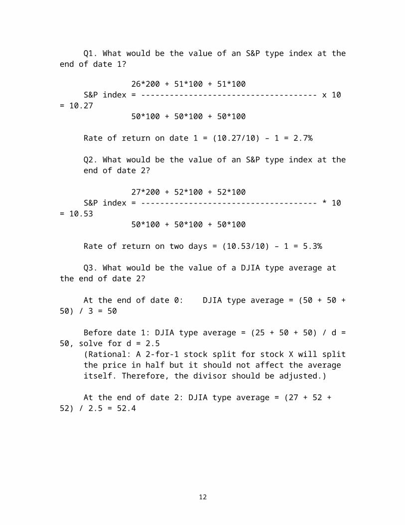
Market indexes, example 1You are given the following information regarding stocks X, Y, and Z:
Stock price # of shares outstandingDate X* Y Z X* Y Z
0 $50 $50 $50 100 100 100 1 26 51 51 200 100 100 2 27 52 52 200 100 100
7

* Stock X has a 2-for-1 stock split before trading on day 1. Date 0 is the base date. The current divisor is 3.0 and the base value for an S&P type of index is supposed to be10.
Q1. What would be the value of an S&P type index at the end of date 1?
26*200 + 51*100 + 51*100S&P index = ------------------------------------- x 10 = 10.27
50*100 + 50*100 + 50*100
Rate of return on date 1 = (10.27/10) – 1 = 2.7%
Q2. What would be the value of an S&P type index at the end of date 2?
27*200 + 52*100 + 52*100S&P index = ------------------------------------- * 10 = 10.53
50*100 + 50*100 + 50*100
Rate of return on two days = (10.53/10) – 1 = 5.3%
Q3. What would be the value of a DJIA type average at the end of date 2?
At the end of date 0: DJIA type average = (50 + 50 + 50) / 3 = 50
Before date 1: DJIA type average = (25 + 50 + 50) / d = 50, solve for d = 2.5(Rational: A 2-for-1 stock split for stock X will split the price in half but it should not affect the average itself. Therefore, the divisor should be adjusted.)
At the end of date 2: DJIA type average = (27 + 52 + 52) / 2.5 = 52.4
Rate of return on two days = (52.4 / 50) – 1 = 4.8%
Market indexes, example 2Consider a price weighted market average composed of three securities, A, B, and C, with prices of 20, 30 and 40 respectively. The current divisor is 3.00. What will be the new divisor if stock B issues a 10% stock dividend?
Answer: closing average before stock dividend = (20 + 30 + 40) / 3.00 = 30.00
Adjust the price of stock B: 30 / (1 + 0.1) = 27.27 (new stock price for B if B issues 10% stock dividend)
Calculate the new divisor: (20 + 27.27 + 40) / d = 30.00 (stock dividend should not affect the closing average) and solve for the new divisor, d = 2.91
8

Derivative marketsDerivative assets or contingent claims: payoffs depend on the prices of other (underlying) assets
Options: the rights to buy or sell an asset at a specified price on or before a specified expiration date (rights)
A call option gives the right to buy an asset A put option gives the right to sell an asset
Example1 - you buy a March 140 IBM call option at $5.00 Call option: right to buyStock option: underlying asset is IBM stockContract size: 100 sharesExercises price: $140 to buy one share of IBM stockExpiration date: the third Friday in MarchOption premium: $500Rationale: you expect IBM stock price is going to rise
Example 2 - you buy a March 25 Intel put option for $2.00Put option: right to sellStock option: underlying asset is Intel stockContract size: 100 sharesExercises price: $25 to sell one share of Intel stockExpiration date: the third Friday in MarchOption premium: $200Rationale: you expect that Intel stock price is going to fall
Futures contracts: call for the exchange of certain goods for cash at an arranged-upon price (future’s price) at a specified future date (obligations)
Example 3 - you buy a June gold futures contract at $1,300 per ounceCommodity futures contract: underlying asset is a commodityContract size: 100 ouncesFutures price: $1,300 per ounce to buy goldDelivery month: JuneRationale: you expect gold price is going to rise
Example 4 - a farmer sells an October corn futures contract at 475 Commodity futures contract: underlying asset is a commodityContract size: 5,000 bushelsFutures price: $4.75 per bushel to sell corn Delivery month: OctoberRationale: the farmer wants to lock in the price, hedging
9

ASSIGNMENTS
1. Concept Checks and Summary2. Key Terms3. Intermediate: 12, 13, 14, 18, 19, and CFA1
10

Chapter 3 - Securities Markets
New issues How securities are traded U.S. securities markets Trading costs Margin trading and short sales
New issuesRecall primary markets and secondary markets
Primary markets: for new issues, either IPOs or existing firms issuing new securities (seasoned offerings)
IPOs: initial public offerings, shares being sold to the public for the first time
Investment banker: firm specializing in the sale of new securities
Underwriting: the process of purchase new shares from the issuing firm and resell the shares to the public
Prospectus: a document that describes the firm issuing the security and provides the information about the firm
Selling process for large new issues: the role of investment bankersUnderwriting; Advising; Distributing
Best efforts vs. underwritten issues
Underwriting syndicate: a group of investment bankers formed by a leading underwriter to spread the financial risk associated with selling new
securities
Issuing firm (Figure 3.1 - Digital Image)
Lead underwriter Underwriting syndicate
Investment banker A Investment banker B Investment banker B
Individual/Private Investors
11
Private placement: new securities are sold directly to a small group of individuals or wealthy investors
Initial return of IPOs: very high first day returns all over the world (Figure 3.2 - Digital Image)
IPOs in the long run: in general poor performance, especially in next three years(Figure 3.3 - Digital Image)
How securities are tradedTypes of markets
Direct search markets: buyers and sellers seek each other directly, which are the least organized markets, for example, a student buys a used car from another student
Brokered markets: brokers offer search services for profits/commissions, for example, the real estate market
Dealer markets: dealers specializing in particular assets buy and sell them in their own accounts for profits, for example, the over-the-counter (OTC) markets
Auction markets: traders converge at one place to buy and sell assets, for example, the New York Stock Exchange (NYSE). Auction markets are the most efficient markets because all traders will get the best price possible.
Types of brokersFull service broker vs. discount broker
Types of accountsCash account vs. margin account (without or with borrowing capacity)
Bid price - the highest price a dealer is willing to pay for a given securityAsked price - the lowest price a dealer is willing to sell a given securityBid-ask spread: the difference of the two prices, which is the profit for a dealer
Types of orders:Market order: to buy or sell at the best price available
Limit order: to buy at or below a specified price or sell at or above a specified price
Stop order (stop-loss order): to sell when price reaches or drops below a specified level or to buy when price reaches or rises above a specified level. It becomes a market order when the stop price is reached.
12

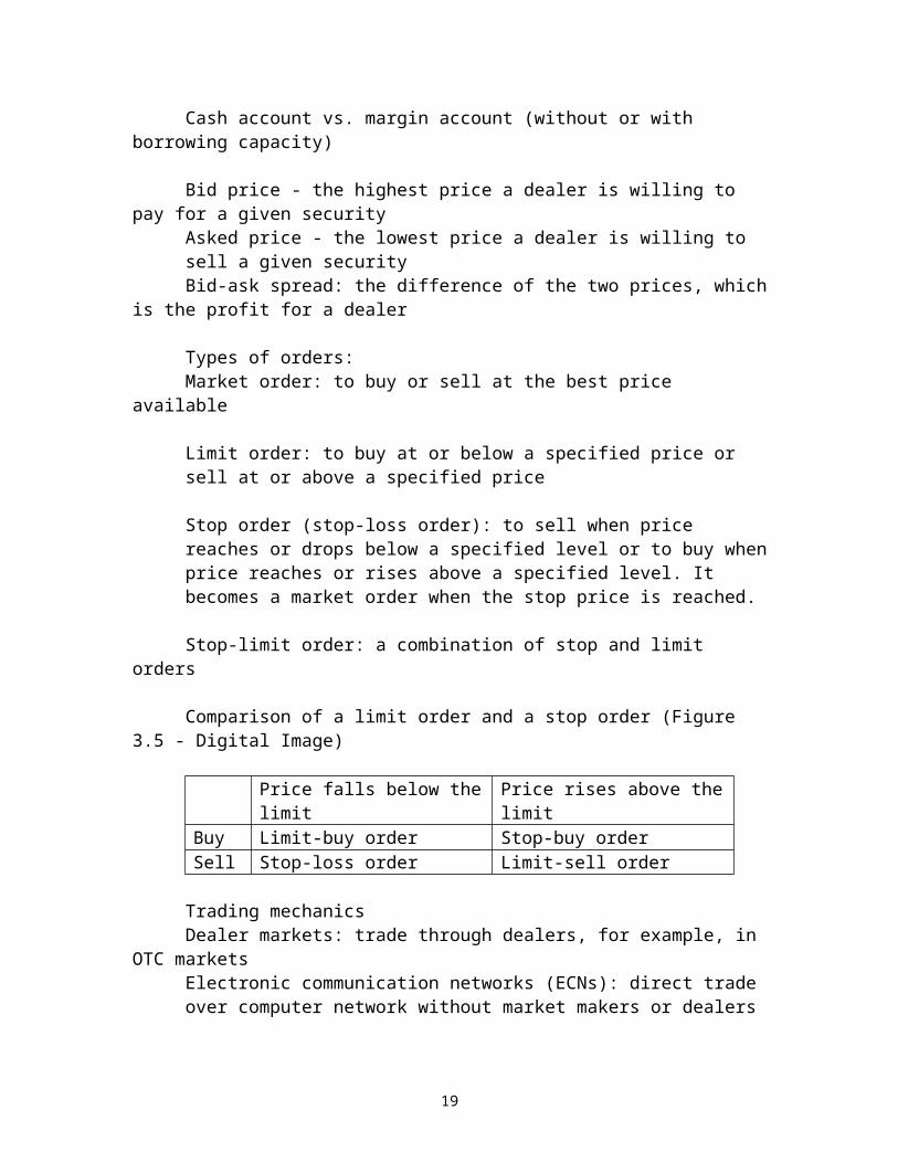
Stop-limit order: a combination of stop and limit orders
Comparison of a limit order and a stop order (Figure 3.5 - Digital Image)
Price falls below the limit Price rises above the limitBuy Limit-buy order Stop-buy orderSell Stop-loss order Limit-sell order
Trading mechanicsDealer markets: trade through dealers, for example, in OTC marketsElectronic communication networks (ECNs): direct trade over computer network without market makers or dealersSpecialist markets: trade through specialists, for example, in NYSE
Specialist: a trader who makes a market in the shares of one or more stocks and maintains a fair and orderly market by dealing personally in the market
U.S. securities marketsNasdaq: National Association Security Dealers Automated Quotations System Nasdaq stock market: a computer-linked price quotation system for the OTC markets with about 3,200 firms listed for trading
NYSE: New York Stock Exchange, the largest exchange in the U.S. with about 2,800 firms listed for trading
Block trade: a large transaction in which at least 10,000 shares of stock are bought or sold
Program trade: a coordinated purchase or sale of an entire portfolio
Settlement: a trade must be settled in 3 working days, called T+3 settlement
Trading costsFull service brokers charge more than discount brokers
Fixed-commission schedule - small transactions, for example, $7.95 a trade for up to 1,000 shares
Negotiated commissions - large transactions (block trade)Explicit vs. implicit costCommissions are explicit costs while bid-ask spread is an implicit (hidden) cost
13
Margin trading and short salesTypes of transactions: Long purchase - direct buyShort selling - sale of borrowed securities
Margins:Margin trading - borrow money and buy stock to magnify returns by reducing the amount of capital that must be put in by investors
Margin requirements - the minimum amount of equity put in by an investor
Initial margin - the minimum amount of equity that must be provided by an investor at the time of purchase, 50% minimum
Maintenance margin - the minimum amount of equity that must be maintained in the margin account at all time, 25% minimum
Margin call - notification of the need to bring additional equity
(1) Buying on margin (borrow money and buy stock):
Market value of stock - Loan Equity in accountMargin = -------------------------------------- = ------------------------------ (1)
Market value of stock Market value of stock
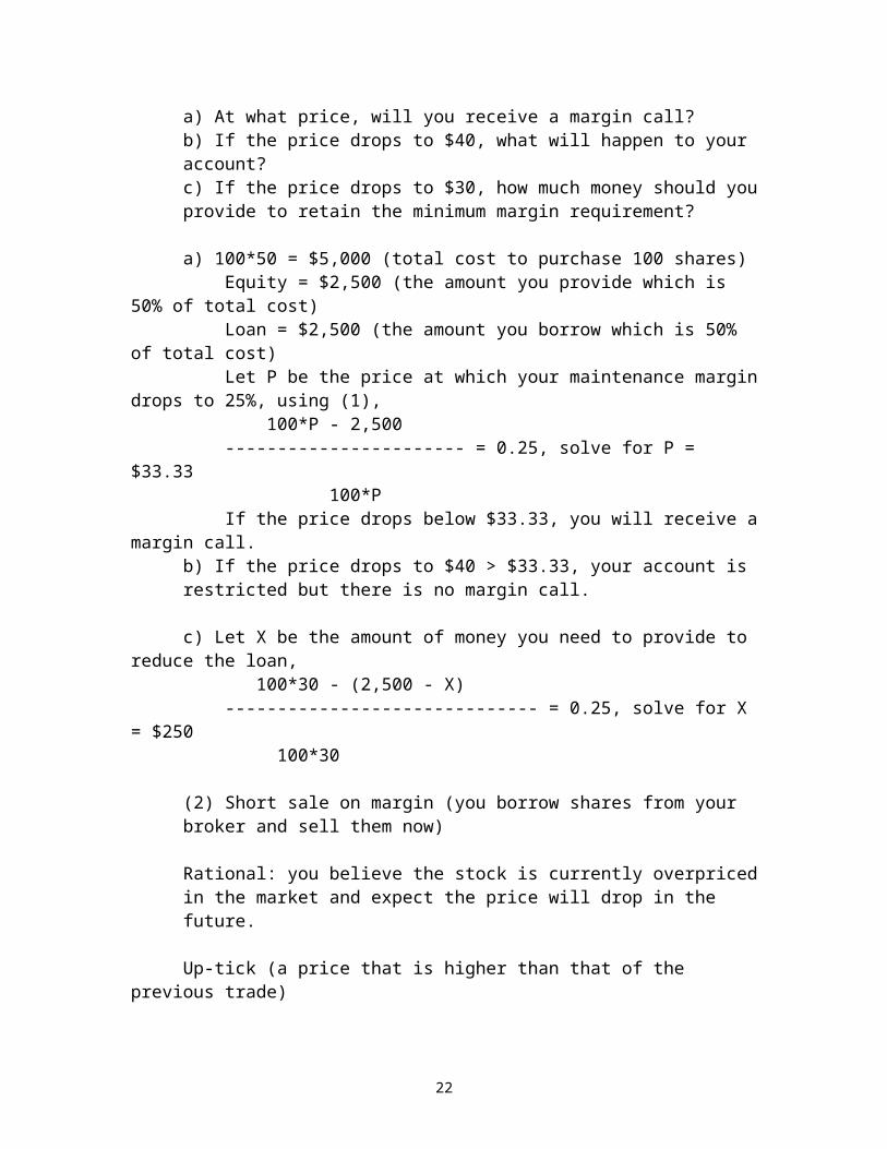
Buying on margin, example 1Suppose you bought 100 shares of XYZ at $50.00 per shares in your margin account. The initial margin is 50% and the maintenance margin is 25%. a) At what price, will you receive a margin call? b) If the price drops to $40, what will happen to your account? c) If the price drops to $30, how much money should you provide to retain the minimum margin requirement?
a) 100*50 = $5,000 (total cost to purchase 100 shares) Equity = $2,500 (the amount you provide which is 50% of total cost) Loan = $2,500 (the amount you borrow which is 50% of total cost) Let P be the price at which your maintenance margin drops to 25%, using (1), 100*P - 2,500 ----------------------- = 0.25, solve for P = $33.33 100*P If the price drops below $33.33, you will receive a margin call.b) If the price drops to $40 > $33.33, your account is restricted but there is no margin call.
c) Let X be the amount of money you need to provide to reduce the loan, 100*30 - (2,500 - X)
14
------------------------------ = 0.25, solve for X = $250 100*30
(2) Short sale on margin (you borrow shares from your broker and sell them now)
Rational: you believe the stock is currently overpriced in the market and expect the price will drop in the future.
Up-tick (a price that is higher than that of the previous trade)Up-tick rule in short sale: a rule designed to restrict short selling from further driving down the price of a stock that has dropped more than 10% in one day. At that point, short selling would be permitted if the price of the security is above the current national best bid (uptick). It will enable long sellers to stand in the front
of the line and sell their shares before any short sellers once the circuit breaker (a 10% drop in one day) is triggered.
Value of assets - Loan EquityMargin = ---------------------------------- = -------------- (2)
Value of stock owed Loan
Short sale on margin, example 2Suppose you short sell 100 shares of ABC at $100 per share in your margin account. The initial margin is 60% and the maintenance margin is 30%. a) At what price, will you receive a margin call? b) What will happen if the price rises to $110 per share? c) If the price drops to $80 per share after your short sale, what is the return from short sale if the interest charge totals $500?
a) 100*100 = $10,000 (short sale proceeds) 10,000*60% = $6,000 (the initial margin you should provide which is 60% of
short sale proceeds) Value of assets = $16,000
Let P be the price at which your margin drops to 30%, using (2), 16,000 - 100*P ------------------------ = 0.30, solve for P = $123.08 100*P
If the price rises above $123.08 you will receive a margin call.
b) If the price rises to $110 < $123.08, your account is restricted but you will not receive a margin call.
Money made 100*(100 - 80) - 500c) Rate of return = ---------------------- = ------------------------------ = 25%
Money invested 6,000
15
ASSIGNMENTS
1. Concept Checks and Summary2. Key Terms3. Intermediate: 14, 15, 21, and CFA 1, 2, 3
16

Chapter 4 - Mutual Funds and Other Investment Companies
Investment companies Mutual funds Costs of investing in mutual funds Mutual fund returns Investing in mutual funds
Investment companiesAn investment company is a type of financial intermediary. It sells itself to the public and uses the funds to invest in a portfolio of securities.
Mutual funds are investment companies (open-end).
Advantages of investing in mutual funds: Economies of scale Professional management Diversification and divisibilityRecord keeping and administration
NAV: the underlying value on a per share basis of a mutual fundIt is determined by the closing-bell prices and it varies every day
NAV = (market value of assets - liabilities) / number of shares outstandingFor example, a mutual fund has $120 million in assets and 5 million of liabilities. If it has 5 million shares outstanding, the net asset value (NAV) is $23 per share.
Managed investment companies: open-end vs. closed-endOpen-end fund: investors can buy shares from or sell shares back to the fund at NAV (it may involve in purchase or redemption charges), with no limit on the number of shares the fund can issue
Closed-end fund: it is traded at prices that can differ from NAV and the number of shares outstanding is fixed
Unit investment trust: money pooled from many investors that is invested in a portfolio fixed for the life of the fund
Hedge fund: a private investment pool, open to wealthy or institutional investors, that is exempt from SEC regulations
Real estate investment trusts (REITs): similar to closed-end funds that invest in real estate or loans secured by real estate
17
Mutual fundsMutual funds are common names for open-end investment companies
More than 90% of mutual funds are open-end funds
Capital gains vs. current income
Investment policy: each fund has its policy contained in the fund’s prospectus
Money market funds: invested in short-term and low-risk instruments
Equity funds: mainly invested in stocks, growth funds vs. income funds
Balanced funds: a balanced return from fixed income securities and long-term capital gains
Bond funds: invested in various bonds, more current income
Index funds: mimic market indexes (for example, S&P 500 index)
Sector funds: restrict investments in particular sectors (for example, financial service sector)
International funds: invested in international stocks
Costs of investing in mutual fundsOperating expenses: costs to operate the fund, including administrative expenses, ranging from 0.2% to 2.0%
Loads: commission charges, sales charges, or redemption charges
Front-end load: deduct a % charge from the initial investment (for example, 5%)
Low-load fund: less than 3% of front charge
Offering price = NAV / (1 – load) or NAV = offering price * (1 - load)
No-load fund: selling at NAV, or offering price = NAV
Back-end load: a commission change on the sale of shares
Other fees: for example, 12b-1 fees to cover marketing and distribution costs
18
Mutual fund returnsSources of return: dividend income; capital gains distributions; unrealized capital
gains
NAV1 – NAV0 + I1 + G1
Rate of return = ------------------------------------- NAV0
I1: income distribution during the periodG1: capital gains distribution during the period
Note: All fees are deducted directly from NAV
Example on return of a mutual fund, problem 4-21 on page 105
At the start of the year: $200 million in assets with no liabilities and 10 million shares outstanding At the end of the year: dividend income $2 million; no capital gains distribution; fund price rises by 8%, and 1% of 12b-1 fees is charged at the end of the year
Answer: NAV0 = $20NAV1 = 20(1.08)*(1-0.01) = $21.384I1 = $0.2 and G1 = 0
21.384 – 20.00 + 0.2Rate of return = ------------------------------ = 7.92%
20.00
Investing in mutual fundsWealth accumulationDiversificationProfessional management Low cost
Speculation and short-term trading
Selection process Objectives What a fund offers – investment policy Main holdingsLoad vs. no-load funds Open-end vs. closed-end funds
19

Taxation on mutual fund income
Turnover ratio: the ratio of the trading activity of a portfolio to the assets of the portfolio
Example: see concept check 4.3
Long-term capital gainsShort-term capital gainsDividends
If it is a retirement account (Roth IRA, regular IRA, 401K or 403B): all taxes are either exempt or deferred
Exchange-traded funds (ETFs): offshoots of mutual funds that allow investors to trade index portfolios, for example, Spider (SPDR) for S&P 500, Diamonds (DIA) for Dow Jones Industrial Average, Qubes (QQQQ) for NASDAQ 100
ASSIGNMENTS
1. Concept Checks and Summary2. Key Terms3. Intermediate: 11, 12, 13, 21, 22, and 24
20

Chapter 5 - Return and Risk
Rates of return Risk and risk premium Historical return Inflation and real return Asset allocation
Rates of returnComponents of return: cash dividend and capital gains (or capital losses)
Total return ($) = return from cash dividend + return from capital gains (or losses)
Total return (%) = dividend yield + capital gain yield
Holding period return (HPR):
Ending price – Beginning price + Cash dividendHPR = --------------------------------------------------------------
Beginning price
Example Div = $4
P0 = $100 P1= $110
0 1
110 – 100 + 4 10 4HPR = ----------------------- = -------- + -------- = 10% + 4% = 14%
100 100 100
Capital gains yield: % change in price, 10%
Dividend yield: % return from dividend, 4%
Returns over multiple periods
Table 5-1: Quarterly cash flows and rates of return of a mutual fund1st quarter 2nd quarter 3rd quarter 4th quarter
Assets at the start of quarter 1.0 mil 1.2 mil 2.0 mil 0.8 milHolding period return (HPR) 10.0% 25.0% (20%) 25.0%Total assets before net inflow 1.1 mil 1.5 mil 1.6 mil 1.0 milNet inflow 0.1 mil 0.5 mil (0.8 mil) 0.0 milAssets at the end of quarter 1.2 mil 2.0 mil 0.8 mil 1.0 mil
21
Arithmetic mean: simple average, the sum of returns in each period divided by the number of periods - best forecast of performance in the future
Arithmetic mean = (10 + 25 – 20 + 25) / 4 = 10%
Geometric mean: time-weighted average return (considers compounding)
(1 + 0.1)*(1+0.25)*(1-0.2)*(1+0.25) = (1 + rG)4
Solve for rG = 8.29%
Dollar-weighted average return: internal rate of return for a project
Quarter0 1 2 3 4
Net cash flow -1.0 -0.1 -0.5 0.8 1.0
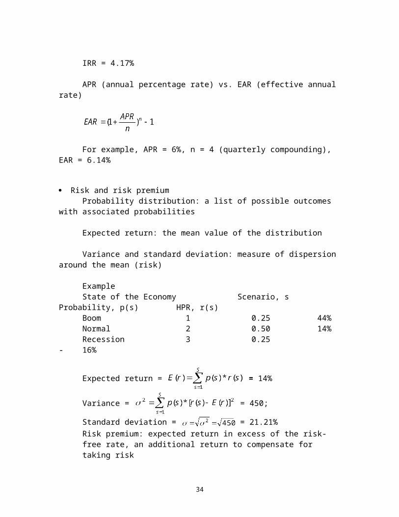
IRR = 4.17%
APR (annual percentage rate) vs. EAR (effective annual rate)
For example, APR = 6%, n = 4 (quarterly compounding), EAR = 6.14%
Risk and risk premiumProbability distribution: a list of possible outcomes with associated probabilities
Expected return: the mean value of the distribution
Variance and standard deviation: measure of dispersion around the mean (risk)
ExampleState of the Economy Scenario, s Probability, p(s) HPR, r(s)Boom 1 0.25 44%Normal 2 0.50 14%Recession 3 0.25 -16%
Expected return = = 14%
Variance = = 450;
Standard deviation = = 21.21%
22

Risk premium: expected return in excess of the risk-free rate, an additional return to compensate for taking risk
Risk aversion: reluctant to accept risk
, where A is the risk aversion coefficient or
For example, if the risk premium is 8%, the standard deviation is 20%, then the risk aversion coefficient A = 4. The higher the risk aversion is for an investor, the higher the value of A, and the higher the risk premium.
Sharpe (reward-to-volatility) measure = S = = = 0.4
(more discussions in Chapter 18)
Historical returnUsing historical data to estimate mean and standard deviation
Example: MO
Historical returns: summary statistics for the U.S market and the world during 1926 - 2008 (Table 5.2 - Digital Image)
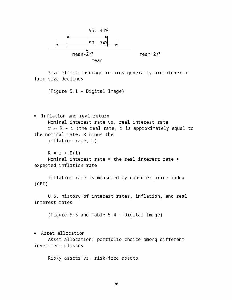
Interpretation of the numbersNormal distribution: 68.26% (1 rule), 95.44% (2 rule), and 99.74% (3
rule)
68. 26%
95. 44% 99. 74%
mean-2 mean+2 mean
Size effect: average returns generally are higher as firm size declines
(Figure 5.1 - Digital Image)
23

Inflation and real returnNominal interest rate vs. real interest rater R – i (the real rate, r is approximately equal to the nominal rate, R minus the inflation rate, i)
R = r + E(i) Nominal interest rate = the real interest rate + expected inflation rate
Inflation rate is measured by consumer price index (CPI)
U.S. history of interest rates, inflation, and real interest rates
(Figure 5.5 and Table 5.4 - Digital Image)
Asset allocationAsset allocation: portfolio choice among different investment classes
Risky assets vs. risk-free assetsAll risky assets form a value-weighted risky portfolio, PAll risk-free assets form a risk-free asset with a risk-free rate, rf
Complete portfolio: a portfolio including risky assets and risk-free assets
Complete portfolio’s expected return and risk:
and
Where E(rc) and c are the expected rate of return and standard deviation for a complete portfolio, E(rp) and p are the expected rate of return and standard deviation for the risky assets, rf is the return on the risk-free asset, y is the weight on risky-assets, and 1-y is the weight on the risk-free asset.
E(rc)
P E(rp) y = 1.5
CALrf
y = 0.5
p
24
The capital allocation line (CAL): a plot of risk-return combinations available byvarying portfolio allocation (weights) between the risk-free asset and the riskyportfolio
Example: E(rp) = 15%, p = 22%, rf = 7%, y = 50%, then
E(rc) = 11%, c = 11%, the Sharpe measure =
Challenge: if y = 1.5 what will happen to the complete portfolio? Where is it located on CAL? What is S? What does it mean (y = 1.5)?
Risk aversion vs. risk tolerance
Passive investment strategy: holding a combination of a well-diversified market portfolio and a risk-free portfolio, assuming all risky assets are fairly priced in the market.
Capital market line (CML): a capital allocation line using the market index portfolio as the risky portfolio (more discussions in Chapters 6 and 7)
E(rc)
M E(rM) y = 1.5
CMLrf
y = 0.5
M
ASSIGNMENTS
1. Concept Checks2. Key Terms3. Intermediate: 5, 6, 12-16, and CFA 1-6
25

Chapters 6&7 - Efficient Diversification, CAPM and APT
Diversification and portfolio risk Portfolio construction with two risky assets Modern portfolio theory Beta coefficient Capital asset pricing model (CAPM) Arbitrage pricing theory (APT)
Diversification and portfolio riskRisk of holding a single asset:
Probability distribution (a revisit)
Expected return: E(r)
Variance ( ) and standard deviation ( )
68. 26%
95. 44% . 99. 74% Mean or E(r)
Mean or E(r) determines the center of the distribution while (or ) determines how wide the distribution is. The large the , the wider the distribution, and the higher the risk.
Risk of holding a portfolio: standard deviation of returns of the portfolio
As the number of stocks increases in a portfolio, the portfolio’s total risk, decreases. It is known as the diversification effect.
Portfolio’s total risk = firm’s specific risk + market risk = Diversifiable risk + non-diversifiable risk = non-systematic risk + systematic risk
(Figure 6.1 - Digital Image)
26
Firm’s specific risk
Market risk
# of securities in a portfolio
Portfolio construction with two risky assetsExample: portfolio construction with two risky assets
State of economy Probability (p) rA rB
Recession 0.3 100% -10%Normal 0.4 15% 0%Boom 0.3 -70% 30%
Estimate the distribution for each stock
E(rA) = 15%, = 4,335 and = 65.84% (refer to Chapter 5)
E(rB) = 6%, = 264 and = 16.25% (refer to Chapter 5)
Estimate the correlation between two risky assets
Covariance: = -1,020
Since = ( )*( )*( ), where is called correlation coefficient
Correlation coefficient, = -0.953
= 1 perfectly and positively; 0 < <1 positively but not perfectly;
= 0 no correlation; -1 < < 0 negatively but not perfectly;
= -1 perfectly and negatively
27
rA rA
*
* * = 1 * * = -1
* * * rB rB
* **
What will the diagrams look like if 0 < <1, -1 < < 0, and = 0?
Portfolio’s return and risk
Three rules for two-risky-assets portfolio
(1) The return on a portfolio is a weighted average of the returns on the component securities (A and B), with the investment proportion as weights;
(2) The expected return on a portfolio is a weighted average of the expected returns on the component securities (A and B), with the investment proportion as weights;
(3) The variance of the portfolio is given by
= =
Suppose you invest 10% in stock A and 90% in stock B. What is the expected rate of return of the portfolio? What is the standard deviation of the return of the portfolio?
E(rp) = 6.9%, = 73.59, and = 8.58%
28

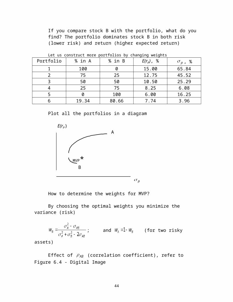
If you compare stock B with the portfolio, what do you find? The portfolio dominates stock B in both risk (lower risk) and return (higher expected return)
Let us construct more portfolios by changing weightsPortfolio % in A % in B E(rp), % , %
1 100 0 15.00 65.842 75 25 12.75 45.523 50 50 10.50 25.294 25 75 8.25 6.085 0 100 6.00 16.256 19.34 80.66 7.74 3.96
Plot all the portfolios in a diagram
E(rp) A
MVP* B
How to determine the weights for MVP?
By choosing the optimal weights you minimize the variance (risk)
; and (for two risky assets)
Effect of (correlation coefficient), refer to Figure 6.4 - Digital Image E(rp)
= -1 A
= 1 = -1
B
29

= -1, perfectly negative correlation, perfect diversification
= 1, perfectly positive correlation, no diversification
-1< <1, there are benefits to diversification. Where negative correlation is present, there will be even greater diversification benefits.
Modern portfolio theoryMarkowitz mean-variance model (for n risky assets)
Efficient portfolio - a portfolio with the highest expected return for a given level of risk or a portfolio with the lowest risk for a given expected return
Efficient frontier – the set of efficient portfolios
MVP – minimum variance (risk) portfolio
Investment opportunity set: the set of all attainable portfolios, including efficient and inefficient portfolios
E(rp)Efficient set
Investment opportunity set
MVP
Inefficient set
Indifference curves: curves describing investor’s preferences for risk and return, or representing a set of combinations of risk and return that provides the same level of satisfaction
Nonsatiation: more is preferred to less
Risk aversion: most investors are risk-averse
Utility: a measure of the level of satisfaction
30
E(rp) I2 I1
Favorite A B
C
D
Mean-variance criterion: investors desire portfolios that lie to the “northwest”, which means that investors prefer higher return with less risk
I2 is preferred to I1 because I2 provides a higher level of satisfaction (lower risk with same return, i.e., A is better than B, or higher return with same risk, i.e., C is better than D)
Choosing the optimal portfolio by combining the indifference curves with the efficient set
E(rp)
O*
O* is the optimal choice (tangency point) where the utility (satisfaction) is maximized
Points to remember: All portfolios on the efficient set are “equally” goodAll risky assets with no borrowing or lending opportunitiesDifferent investors may have different estimated efficient setDifferent investors may have different indifference curves
31

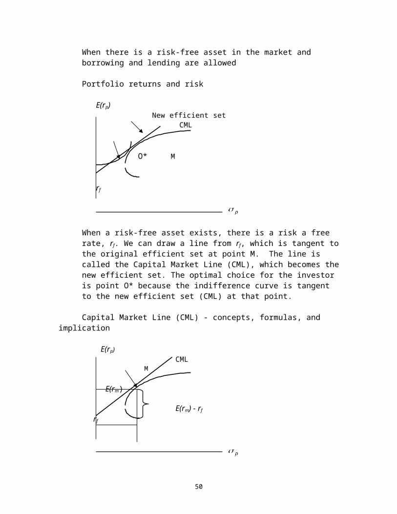
When there is a risk-free asset in the market and borrowing and lending are allowed
Portfolio returns and risk
E(rp)New efficient set CML
O* M
rf
When a risk-free asset exists, there is a risk a free rate, rf. We can draw a line from rf, which is tangent to the original efficient set at point M. The line is called the Capital Market Line (CML), which becomes the new efficient set. The optimal choice for the investor is point O* because the indifference curve is tangent to the new efficient set (CML) at that point.
Capital Market Line (CML) - concepts, formulas, and implication
E(rp)CML
M
E(rm)
E(rm) - rf
rf
: It is the Capital Market Line (CML) formula
CML has the risk-free rate as the intercept and the reward-to-variability ratio as the slope
32

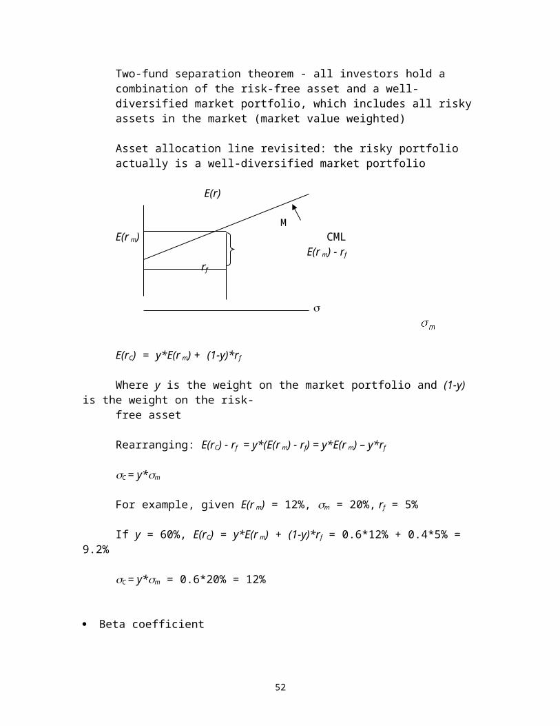
Two-fund separation theorem - all investors hold a combination of the risk-free asset and a well-diversified market portfolio, which includes all risky assets in the market (market value weighted)
Asset allocation line revisited: the risky portfolio actually is a well-diversified market portfolio
E(r)
ME(r m) CML
E(r m) - rf
rf
E(rC) = y*E(r m) + (1-y)*rf
Where y is the weight on the market portfolio and (1-y) is the weight on the risk-free asset
Rearranging: E(rC) - rf = y*(E(r m) - rf) = y*E(r m) – y*rf
C = y*m
For example, given E(r m) = 12%, m = 20%, rf = 5%
If y = 60%, E(rC) = y*E(r m) + (1-y)*rf = 0.6*12% + 0.4*5% = 9.2%
C = y*m = 0.6*20% = 12%
Beta coefficientA measure of the market risk (systematic risk) for a stock or a portfolio
Characteristic line (CL): a regression line used to estimate the beta coefficient
The slope of the CL is the estimated beta coefficient for stock i
Example: MOSingle index model
33
Asset returns are related to the returns of a market index
Excess return: rate of return in excess of the risk-free rate (R = r - rf)
, where is an error term and the average of error terms is zero.
Ri
*
ai
Rm
Taking the variance on both sides of the single index model:
Total risk = market risk + specific risk = systematic risk + firm’s specific risk
is the proportion of total variance attributed to market fluctuations
Example: In a CAPM equilibrium, the risk-free rate is 5% and the expected rate of return on the market is 10% with a standard deviation of 18% ( = 18%). A common stock i has an expected return of 12% with a standard deviation of 30% (
= 30%). What percentage of the total risk for stock i is the firm’s specific risk? What percentage is due to the market risk?
AnswerStep 1: Solve for the beta of stock i, using CAPM
12% = 5% + i (10% - 5%), solving for i = 1.4
Step 2: Solve for the firm’s specific risk, using the formula above,900 = (1.4)2(18) 2 + , solving for = 264.96
Step 3: Calculate the percentages,264.96/900 = 29.44% (firm’s specific), 635.04/900 = 70.56% (market)
34

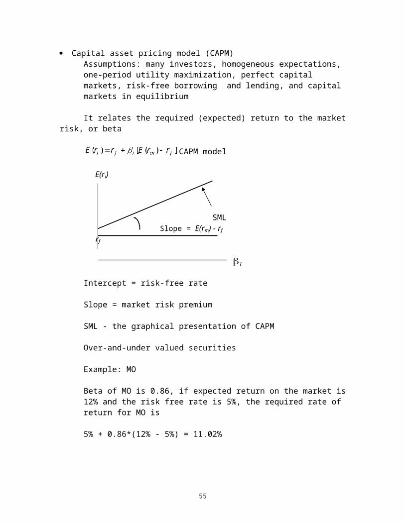
Capital asset pricing model (CAPM)Assumptions: many investors, homogeneous expectations, one-period utility maximization, perfect capital markets, risk-free borrowing and lending, and capital markets in equilibrium
It relates the required (expected) return to the market risk, or beta
CAPM model
E(ri)
SML Slope = E(rm) - rf
rf
Intercept = risk-free rate
Slope = market risk premium
SML - the graphical presentation of CAPM
Over-and-under valued securities
Example: MO
Beta of MO is 0.86, if expected return on the market is 12% and the risk free rate is 5%, the required rate of return for MO is
5% + 0.86*(12% - 5%) = 11.02%
Checking the average return over the past 5 years we find that it is 1.22% per month or 14.64% per year (simple interest)
The stock’s alpha = 14.64% – 11.02% = 3.62% (under priced) since the realized return is higher than the CAPM predicts (above the SML)
Limitations with CAPM: rely on the market portfolio and expected returns
35
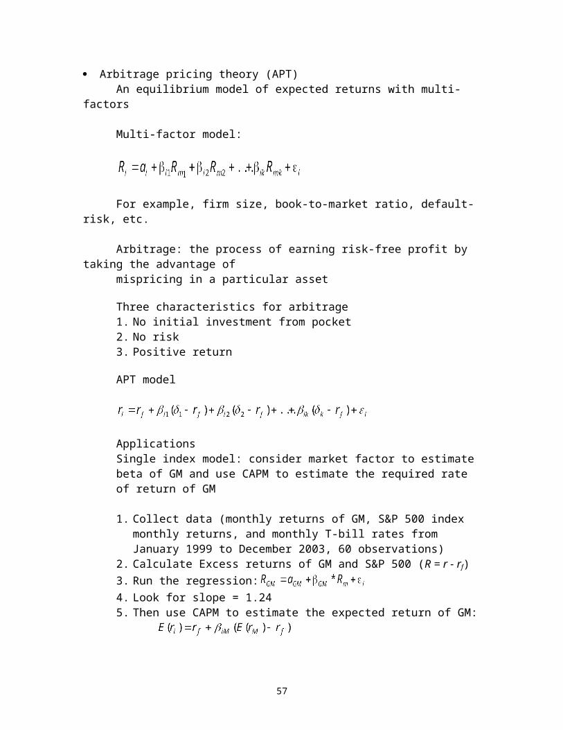
Arbitrage pricing theory (APT)An equilibrium model of expected returns with multi-factors
Multi-factor model:
For example, firm size, book-to-market ratio, default-risk, etc.
Arbitrage: the process of earning risk-free profit by taking the advantage of mispricing in a particular asset
Three characteristics for arbitrage1. No initial investment from pocket2. No risk3. Positive return
APT model
ApplicationsSingle index model: consider market factor to estimate beta of GM and use CAPM to estimate the required rate of return of GM
1. Collect data (monthly returns of GM, S&P 500 index monthly returns, and monthly T-bill rates from January 1999 to December 2003, 60 observations)
2. Calculate Excess returns of GM and S&P 500 (R = r - rf)3. Run the regression:4. Look for slope = 1.245. Then use CAPM to estimate the expected return of GM: 6. Assume rf = 4.00%, market risk premium = 5.5%, expected return = 10.82%
Two factor model of Merton: consider market factor and interest rate factor to estimate betas and use multifactor model to estimate expected return of GM
1. Collect data2. Run the regression: to estimate betas3. Use the two-factor model to estimate expected rate of return
36

Assume that the risk-free rate is 4.00%, the expected market risk premium is 6% and the expected interest rate risk premium is 3%. If the market beta of stock i is 1.2 and interest rate beta of the stock is 0.7, the expected return for stock i is
E(ri) = 4% + 1.2*(6%) + 0.7*(3%) = 13.3%
Three factor model of Fama and French: considers market factor, size factor, and book-to-market ratio
1. Collect data and run a multifactor regression: to estimate betas for
stock i2. Use three-factor model to estimate expected rate of return for stock i 3. Assuming for Dell (using monthly data over the period 2002-2006), , , and From French’s website, , , and , then Dell’s expected risk premium 1.132*7.99% - 0.8026*4.40% + 0.2742*2.94% = 6.32%
ASSIGNMENTS
Chapter 61. Concept Checks2. Key Terms3. Intermediate: 8-12 and CFA 1-3
Chapter 71. Concept Checks2. Key Terms3. Intermediate: 4-7, 17-19, and CFA 1-14
37

Chapter 8 - Market Efficiency
Random walks and efficient market hypothesis (EMH) Implications of EMH The role of portfolio manager in an efficient market Evidence of market efficiency and anomalies Interpretation of EMH
Random walks and efficient market hypothesis (EMH)Random walk: stock price changes are random and unpredictableEfficient market: prices of securities in the market fully and quickly reflect all available information, which means that there is no arbitrage opportunity
Figures 8.1 and 8.2 - Digital Image
Forms of efficiency:Weak-form efficiency: stock prices already reflect all information contained in
the history of past trading
Semistrong-form efficiency: stock prices already reflect all publicly available information in the market
Strong-form efficiency: stock prices already reflect all relevant information in the market, including inside information
Implications of EMHTechnical analysis vs. fundamental analysis
Technical analysis: research on recurrent and predictable patterns in the market
Relative strength: compare the recent performance of a stock with that of the market or other stocks
Resistance level: a price level above which it is supposedly unlikely for a stock or stock index to rise
Support level: a price level below which it is supposedly unlikely for a stock or stock index to fall
Moving averages: 50-day and 200-day moving averages
If the market is efficient, what will happen to technical analysis?
38

Fundamental analysis: research on determinants of stock value, such as earnings and dividends prospects, expectations of future interest rates, and risk of the firm
Active vs. passive portfolio management
Active: search for mispriced (overvalued or undervalued) securities, buy and sell often to timing the market
Passive: buy and hold a well-diversified portfolio, buy and hold strategy
The role of portfolio manager in efficient marketDiversification to reduce firm’s specific risks
Tax consideration for different investors
Resource allocation
Demand for investment varies with age, tax bracket, risk aversion, and employment, etc., so portfolio managers can tailor portfolios for different investors.
Evidence of market efficiency and anomaliesThree main issues(1) The magnitude issue: fund managers deal with portfolios worth hundreds of
millions. Only one tenth of 1% will be worth a lot.(2) Selection bias: if a manager knows a way to make money for sure, he/she
will keep it secret.(3) Lucky event: sometimes, a fund has a superior performance. It can just be a
lucky event (bet the right stocks).
Weak-form tests: patterns in stock returnsSerial correlation test: involves measuring the correlation between stock returns for various lags and the results indicate fairly weak and positive correlation for short-horizon returns and fairly strong and negative correlation for long-horizon returns
Momentum effect: the tendency of poorly-performing stocks and well-performing stocks in one period to continue that abnormal pattern in following periods
Buying past winners and selling past losers will make abnormal profits
Reversal effect: the tendency of poorly performing stocks and well-performing stocks in one period to experience reversals in the following periodImplication: short- and intermediate-horizon momentum and long-run reversal
39

Semi-strong form tests: market anomaliesAnomalies: patterns that seem to contradict the EMH
P/E ratio effect: low P/E ratio stocks have earned higher average risk-adjusted returns than high P/E ratio stocks
Small-firm effect: small firm stocks have earned higher abnormal returns, primary in January
Figure 8.3 - Digital Image
Neglected-firm effect: less well-known firm stocks have earned abnormal returns
Book-to-market effect: high book-to-market value stocks have earned abnormal returns
Figure 8.4 - Digital Image
Post-earnings-announcement price effect: stock prices don’t reflect new information rapidly
Figure 8.5 - Digital Image
Strong-form tests: inside informationInsiders make superior profits with inside information: the market is not strong-form efficient
Interpretation of EMH Risk premium or inefficiency?
For example, Fama and French’s three factor model indicates higher returns are associated with more risks
Anomalies or data mining?
ASSIGNMENT
1. Concept Checks2. Key Terms3. Intermediate: 10-16 and CFA 1-6
40

Chapters 10&11 - Debt Securities
Bond characteristics Interest rate risk Bond rating Bond pricing Term structure theories Bond price behavior to interest rate changes Duration and immunization Bond investment strategies
Bond characteristicsBond: long-term debt security that the issuer makes specified payments of interest (coupon payments) over a specific time period and repays a fixed amount of principal (par or face value) at maturity
Face value or par value: usually $1,000
Coupon rate and interest payment
Zero-coupon bond: coupon rate is zero, no coupon payment, sells at a discount. For example: a 10 year zero-coupon bond sells at $550 and yields 6.16% per year
Maturity date
Call provision: the issuer can repurchase bonds during the call period
Call premium and call price
Convertible bonds: can be converted into common stocks
Puttable bonds: bondholders can sell bonds back to the issuer before maturity
Floating-rate bonds: coupon rates vary with some market rates
Indexed bonds: payments are tied to a general price index
Junk bonds: high yields with high default risk
Government bonds, corporate bonds, international bonds
Preferred stocks: hybrid security, often considered as an equity but usually included in fixed-income securities
41

Interest rate risk Interest rate price risk vs. interest rate reinvestment risk (reinvestment risk)
Interest rate price risk: risk that a bond value (price) falls when market interest rates rise
Reinvestment risk: risk that the interests received from a bond will be reinvested at a lower rate if market interest rates fall
Bond rating Letter grades that designate quality (safety) of bonds (Figure 10.8 - Digital
Image)AAA AA Investment grade bonds with low default risk A BBB BB B Speculative grade (junk) bonds with high default risk .
Why bond rating? Firm's credit; Borrowing capacity
Determinants: Coverage ratios - ratios of earnings to fixed costsLeverage ratio - debt to equity ratioLiquidity ratios - current ratio and quick ratioProfitability ratios - ROA and ROE Cash-flow-to debt ratio - ratio of total cash to outstanding debt
Bond pricingAccrued interest and quoted price
Invoice price = quoted (flat) price + accrued interest0 182 days 40 days 142 days remaining until next coupon
Suppose annual coupon is $80 and the quoted price is $990,
Invoice price = 990 + (40/182)*40 = $998.79
Bond price = present value of coupons + present value of par value
The required rate of return serves as the discount rate
42

Premium bonds vs. discount bondsA premium bond sells for more than its face value ($1,000)A discount bond sells for less than its face value ($1,000)
Annual interest payment valuation model
P = present value of coupons + present value of par value = C (PVIFAr,n) + PV (PVIFr,n),
P: intrinsic value of the bond C: annual coupon paymentr: the required rate of return, the market interest rate for the bondn: the number of years until the bond maturesPV: par value (face value, $1,000 usually)
Semiannual interest payment valuation model: adjust the annual coupon to semiannual (C to C/2), the annual required rate of return to semiannual (r to r/2), and the number of years to maturity to semiannual periods (n to 2n)
Overpriced securities vs. underpriced securitiesIf the intrinsic value > the market price, the bond in the market is underpricedIf the intrinsic value < the market price, the bond in the market is overpricedIf the intrinsic value = the market price, the bond in the market is fairly priced
Example: A 30-year 8% coupon bond pays semiannual coupon payments. The market interest rate (required rate of return) on the bond is 10%. What should be the bond price (fair value)? If the market price of the bond is $850.00, should you buy the bond?
Answer: n = 60, i/y = 5%, FV = 1,000, PMT = 40, solve for PV = -810.71No, you should not buy the bond since the intrinsic value ($810.71) < the market price ($850.00)
If the market interest rate for the bond is 8%, what should be the bond price?Answer: PV = -1,000
If the market interest rate for the bond is 7%, what should be the bond price?Answer: PV = -1,124.72
Bond price and market interest rates have an inverse relationship: keeping other things constant, the higher the market interest rate, the lower the bond price(Figure 10.3 - Digital Image)
43
Yield to maturity (YTM): rate of return from a bond if it is held to maturity
Example (continued): what is YTM of the bond?
Answer: PV = -850, FV = 1,000, PMT = 40, n = 60, solve for i/y = 4.76%, YTM = 4.76*2 = 9.52%
Yield to call (YTC): rate of return from a bond until it is called
Example (continued): suppose the bond can be called after 5 years at a call price of $1,050, what is YTC?Answer: PV = -850, FV = 1,050, PMT = 40, n = 10, solve for i/y = 6.45%, YTC = 6.45*2 = 12.91%
Current yield (CY): annual coupon payment divided by the current bond priceExample (continued): what is the current yield of the bond?CY = 80/850 = 9.41%
If market interest rates rise what would happen to the current yield of a bond?
Answer: the current yield would increase since the bond price would decrease
Realized compound return: compound rate of return on a bond with all coupons reinvested until maturity
Example: 10.5 (Figure 10.5 - Digital Image)Consider a two-year bond selling at par and paying 10% coupon once a year. The YTM is 10%. If the coupon payment is reinvested at an interest rate of 8% per year, the realized compound return will be less than 10% (actually it will be 9.91%)
Term structure theoriesTerm structure of interest rates: relationship between time to maturity and yields for a particular fixed-income security
Yield curve: a graphical presentation of the term structure
Expectation theory: the yield curve is determined solely by expectations of future short-term interest rates
Forward rates: implied short-term interest rates in the future
44

Example: suppose that two-year maturity bonds offer yields to maturity of 6% and three-year bonds have yields of 7%. What is the forward rate for the third year?
Using the formula: and solving for fn = 9.02%
Approximation: fn = 7%*3 – 2*6% = 9.00%
Liquidity preference theory: investors demand a risk premium on long-term bonds
Liquidity premium: the extra expected return to compensate for higher risk of holding longer term bonds
Market segmentation theory: investors have their preferences to specific maturity sectors and unwilling to shift from one sector to another
Bond price behavior to interest rate changes (1) The value of a bond is inversely related to its yield.: As yields increase,
bond prices fall; as yields fall, bond prices rise.
(2) An increase in a bond’s yield to maturity results in a smaller price change than a decrease in yield of equal magnitude.
(3) As the maturity date approaches, the value of a bond approaches to its par value.
(4) Prices of long-term bonds tend to be more sensitive to interest rate changes than prices of short-term bonds.
(5) The sensitivity of bond prices to changes in yields increases at a deceasing rate as maturity increases.
(6) Interest rate risk is inversely related to the bond’s coupon rate. Prices of low-coupon bonds are more sensitive to changes in interest rates than prices of high-coupon bonds.
(7) The sensitivity of a bond’s price to a change in its yield is inversely related to the yield to maturity at which the bond is currently selling. (Figure 11.1 - Digital Image)
45

Duration and immunizationDuration: a measure of the effective maturity of a bond, defined as the weighted average of the times until each payment is made, with weights proportional to the present value of the payment.
Measuring duration: Macaulay duration = D = , where
Note: T is the number of years until the bond matures, y is the yield to maturity, and P0 is the market price of the bond
Example: A 3-year bond with coupon rate of 8%, payable annually, sells for $950.25 (face value is $1,000). What is yield to maturity? What is D?
Answer: y = 10%, D = 2.78 years (Spreadsheet 11.1 - Digital Image)
Relationship between duration and bond price volatility
= - D = - D* y
where D* = , is the modified duration
Example (continued): What is D*?
Answer: D* = D/(1+y) = 2.53 years
If the yield drops by 1%, what will happen to the bond price?
Answer: the price will increase by 2.53%
If the yield rises by 1%, what will happen to the bond price?
Answer: the price will decrease by 2.53%
Rules for duration (1) for a zero-coupon bond, the duration is equal to the time to maturity
(2) the lower the coupon rate, the higher the D(3) the longer the time to maturity, the higher the D(4) the lower the yield, the higher the D(5) for a perpetuity, the D = (1+y)/y
46

Bond immunization: a strategy to shield net worth from interest rate movements; to get interest rate price risk and interest rate reinvestment risk to cancel each other over a certain time period to meet a given promised stream of cash outflows
See the example (Table 11.4 - digital Image)
Note: immunization works only for small changes in interest rates
Cash flow matching: matching cash flows from a fixed-income portfolio with those of an obligation
Dedication strategy: refers to multi-period cash flow matching
Application of bond immunization: banking management, pension fund management
Bond investment strategiesPassive strategy: lock in specified rates given the risk, or buy and hold
Active management strategy: more aggressive and risky; try to timing the market
Bond swaps: an investment strategy where an investor liquidates one bond holding and simultaneously buys a different issue (more in FIN 436)
Interest rate swaps: a contract between two parties to exchange a series of cash flows based on fixed-income securities (more in FIN 436)
Tax swaps: replace a bond that has a capital loss for a similar security in order to offset a gain in another part of an investment portfolio
ASSIGNMENTS
Chapter 101. Concept Checks2. Key Terms3. Intermediate: 10-15, CFA 1 and 5
Chapter 111. Concept Checks2. Key Terms3. Intermediate: 10-11, CFA 1-2, and 10
47

Chapter 12 - Macroeconomic and Industry Analysis
Global economy Domestic macro economy Industry analysis Company analysis
Global EconomyTop-down analysis starts with the global economy: overview of the economic conditions around the world
Exchange rate and exchange rate risk
Political risk (country risk)
Domestic macro economyTo develop an economic outlook for domestic economy
Gross domestic product (GDP): total value of goods and services producedHigh grow rate of GDP indicates rapid expansion – check for inflation Negative grow rate of GDP indicates contraction – check for recession
Demand and/or supply shocks
Unemployment rate
Inflation: general level of prices for goods and services
Interest ratesNominal interest rates vs. real interest rates (Figure 12.3 - Digital Image)
Determinants of interest ratesSupply side: from savers, mainly householdsDemand side: from borrowers, mainly businessGovernment side: borrower or saver, through FedThe expected inflation rate
Budget deficit: spending exceeds revenue
Sentiment: optimism or pessimism of the economy
Federal government policy: fiscal and monetary policies
Fiscal polity - the government uses spending and taxing to stabilize the economy
48

Monetary policy – the Fed uses money supply and interest rate to stabilize the economy (price level)
Consumer spending
Exchange rates
Business cycle: repetitive cycles of recession and recovery (Figure 12.4 - Digital Image)
Peak vs. trough
Cyclical industries: with above average sensitivity to the state of the economy
Defensive industries: with below average sensitivity of the state of the economy
Economic indicators (Table 12.2 - Digital Image)Leading indicators: rise or fall in advance of the rest of the economy Coincident indicators: rise or fall with the economy Lagging indicators: rise or fall following the economy
Industrial analysisTo develop an industrial outlook
NAICS code to classify industries (Table 12.3 - Digital Image)
Sensitivity to the business cycle
Sector rotation
Industry life cycle
Industry structure and performanceThreat of entry; Competitors; Substitutes; Bargaining power
Technology development
Future demand
Labor problem
Regulations
49
Company analysisFundamental analysis: intrinsic value, financial statements, ratio analysis, earnings and growth forecast, P/E ratio, and required rate of return (risk)
Valuation models (covered in Chapter 13)
ASSIGNMENT
4. Concept Checks5. Key Terms6. Intermediate: 12, 14, and CFA 6
50

Chapter 13 - Equity Valuations
Characteristics of common stock Valuation by comparables Dividend discount model (DDM) Alternative models Free cash flow valuation approach
Characteristics of common stocksOwnership with residual claims
Advantages and disadvantages of common stock ownershipHigher returnsEasy to buy and sell (liquidity) Higher riskLess current income
Cash dividend, stock dividend, and stock split
Treasury stocks - repurchased stocks held by a firm
Capital gains yield and dividend yield
Valuation by comparablesStocks with similar characteristics should sell for similar prices
Book value: the net worth of common equity according to a firm’s balance sheet
Liquidation value: net amount that can be realized by selling the assets of a firm and paying off the debt
Replacement cost: cost to replace a firm’s assets
Tobin’s q: the ratio of market value of the firm to replacement cost
P/E ratio approachPrice-to-sales ratio approachMarket-to-book value approachPrice-to-cash flow approach
Example (Table 13.1 - Digital Image)
Dividend discount model (DDM)
51
Market price vs. intrinsic value
Market price: the actual price that is determined by the demand and supply in the market
Intrinsic value: the present value of a firm’s expected future net cash flows discounted by the required rate of return
In market equilibrium, the required rate of return is the market capitalization rate
Net income, retained earnings, and cash dividends
General formula:
Forecasting sales and growth rate: g = ROE * b (b is the retention ratio)
Estimating EPS and DPS
(1) Zero growth DDM (g = 0), which means that dividend is a constant (D)
or
where k is the required rate of return and E(r) is the expected rate of return
Example: if D = $2.00 (constant) and k = 10%, then V0 = $20.00
Preferred stocks can be treated as common stocks with zero growth (g = 0)
(2) Constant growth DDM (g = a constant)
D1 = D0*(1+g)D2 = D1*(1+g) = D0*(1+g)2, and in general, Dt = Dt-1*(1+g) = D0*(1+g)t
or
Example: assume D0 = 3.81, g = 5%, k = 12%, then V0 = 57.15
52

Stock price and PVGO (present value of growth opportunity)
Dividend payout ratio (1-b) vs. plowback ratio (b, earnings retention ratio)
Price = no-growth value per share + PVGO
, where is the no-growth value per share
Example: assume E1 = $5.00, k = 12.5%, ROE = 15%
If D1 = $5.00, then g = 0% (g = ROE * b, b = 0)
P0 = 5/0.125 = $40.00
If b = 60%, then g = 15%*0.6 = 9%, D1 = 5*(1-0.6) = $2.00
P0 = $57.14 (from constant DDM)
PVGO = 57.14 – 40.00 = $17.14
(3) Life cycle and multistage growth models: the growth rates are different at different stages, but eventually it will be a constant
Two-stage growth DDMExample: Honda Motor Co.Expected dividend in next four years:$0.90 in 2009 $0.98 in 2010 $1.06 in 2011 $1.15 in 2012Dividend growth rate will be steady beyond 2012
Assume ROE = 11%, b = 70%, then long-term growth rate g = 7.7%
Honda’s beta is 1.05, if the risk-free rate is 3.5% and the market premium is 8%, then k = 11.9% (from CAPM)
Using constant DDM, P2010 = 1.15*(1 + 0.077) / (0.119 - 0.077) = $29.49
$29.49 $0.90 $0.98 $1.06 $1.15 2008 2009 2010 2011 2012
Discount all the cash flows to the present at 11.9%, V2008 = $21.88
Multistage growth DDM: extension of two stage DDM
53

Alternatives modelsP/E ratio approachIf g = ROE*b, the constant growth DDM is
, with k>ROE*b.
Since P/E ratio indicates firm’s growth opportunity, P/E over g (call PEG ratio) should be close to 1.
If PEG ratio is less than 1, it is a good bargain. For the S&P index over the past 20 years, the PEG ratio is between 1 and 1.5.
Price-to-book ratio approach
Price-to-cash flow ratio approach
Price-to-sales ratio approach
Free cash flow valuation approachFree cash flow: cash flow available to the firm or to the shareholders net of capital expenditures
Free cash flow to the firm (FCFF)FCFF = EBIT*(1-tc) + depreciation – capital expenditures – increase in NWC
Use FCFF to estimate firm’s value by discounting all future FCFF (including a terminal value, PT) to the present
Free cash flow to equity holdersFCFE = FCFF – interest expense*(1-tc) + increases in net debt
Use FCFE to estimate equity value by discounting all future FCFE (including a terminal value, PT) to the present
Examples
ASSIGNMENTS
1. Concept Checks2. Key Terms3. Intermediate: 12, 13, 14, and CFA 1-4
54
Chapter 18 - Portfolio Performance and Evaluation
Risk-adjusted returns M2 measure T2 measure Active and passive portfolio management Market timing
Risk-adjusted returnsComparison groups: portfolios are classified into similar risk groups
Basic performance-evaluation statisticsStarting from the single index model
Where is the portfolio P’s excess return over the risk-free rate, is the excess return on the market portfolio over the risk-free rate, is the portfolio beta (sensitivity), is the nonsystematic component, which includes the portfolio’s alpha and the residual term (the residual term has a mean of zero)
The expected return and the standard deviation of the returns on portfolio P
and
Estimation procedure
(1) Obtain the time series of RPt and RMt (enough observations)
(2) Calculate the average of RPt and RMt ( and )
(3) Calculate the standard deviation of returns for P and M ( and )
(4) Run a linear regression to estimate
(5) Compute portfolio P’s alpha:
(6) Calculate the standard deviation of the residual:
55

Risk-adjusted portfolio performance measurement (Table 18.1 - Digital Image)
(1) The Sharpe measure: measures the risk premium of a portfolio per unit of total risk, reward-to-volatility ratio
Sharpe measure =
(2) The Jensen measure (alpha): uses the portfolio’s beta and CAPM to calculate its excess return, which may be positive, zero, or negative. It is the difference between actual return and required return
(3) The Treynor measure: measures the risk premium of a portfolio per unit of systematic risk
Treynor measure =
M2 measureM2 measure: is to adjust portfolio P such that its risk (volatility) matches the risk (volatility) of a benchmark index, then calculate the difference in returns between the adjusted portfolio and the market
Example: Given the flowing information of a portfolio and the market, calculate M2, assuming the risk-free rate is 6%.
Portfolio (P) Market (M)Average return 35% 28%Beta 1.2 1.0Standard deviation 42% 30%
S for P = (0.35 - 0.06) / 0.42 = 0.69
S for M = (0.28 - 0.06) / 0.30 = 0.73
M2 = (0.69 - 0.73)*0.30 = -0.0129 = -1.29%
(Figure 18.2 - Digital Image)
E(r) CML
56
rP = 35% P
M rM = 28% rP* =26.71% M2 CAL P*
rf = 6%
=30% =42%
Alternative way: adjust P to P* (to match the risk of the market)
Determining the weights to match the risk of the market portfolio30/42 = 0.7143 in portfolio1-0.7143 = 0.2857 in risk-free assetAdjusted portfolio risk = 30%Adjusted portfolio return = 0.7143*35% + 0.2857*6% = 26.71% < 28%
M2 = 26.7% – 28% = -1.29%
The portfolio underperforms the market
T2 measureT2 measure: is similar to M2 measure but by adjusting the market risk - beta
Example (continued)
Weights: 1/1.2 = 0.8333 in P and 1 – 0.8333 = 0.1667 in risk-free asset
The adjusted portfolio has a beta of 1: 1.2*0.8333 + 0*0.1667 = 1
Adjusted portfolio return = 0.8333*35% + 0.1667*6% = 30.17% > 28%
T2 = 30.17% – 28% = 2.17%
57

E(r) P rP = 35%
P* rP* = 30.17% rM = 28% T2 SML M
rf = 6%
=1 =1.2
The portfolio outperforms the market
Why M2 and T2 are different?
Because P is not fully diversified and the standard deviation is too high
Active and passive portfolio managementActive: attempt to improve portfolio performance either by identifying mispriced securities or by timing the market; it is an aggressive portfolio management technique
Passive: attempt of holding diversified portfolios; it is a buy and hold strategy
Market timingA strategy that moves funds between the risky portfolio and cash, based on forecasts of relative performance (Table 18.7 - Digital Image)
When can we time the market?
(Figure 18.9 - Digital Image)
Can we time the market?
58

Example: Intermediate 6 (Figure - Digital Image)
We first distinguish between timing ability and selection ability. The intercept of the scatter diagram is a measure of stock selection ability. If the manager tends to have a positive excess return even when the market’s performance is merely “neutral” (i.e., the market has zero excess return) then we conclude that the manager has, on average, made good stock picks. In other words, stock selection must be the source of the positive excess returns.
Timing ability is indicated by the curvature of the plotted line. Lines that become steeper as you move to the right of the graph show good timing ability. The steeper slope shows that the manager maintained higher portfolio sensitivity to market swings (i.e., a higher beta) in periods when the market performed well. This ability to choose more market-sensitive securities in anticipation of market upturns is the essence of good timing. In contrast, a declining slope as you move to the right indicates that the portfolio was more sensitive to the market when the market performed poorly, and less sensitive to the market when the market performed well. This indicates poor timing.
We can therefore classify performance ability for the four managers as follows:
Selection Ability Timing AbilityA Bad GoodB Good GoodC Good BadD Bad Bad
ASSIGNMENTS
1. Concept Checks2. Key Terms3. Intermediate: 5, 6, and CFA 1-4
59

Chapter 19 - International Investing
Global equity markets Risk factors in international investing International diversification Exchange rate risk and political risk
Global equity marketsDeveloped markets vs. emerging markets
(Tables 19.1 and 19.2 - Digital Image)
Market capitalization and GDP: positive relationship, the slope is 0.66 and R2 is 0.28, suggesting that an increase of 1% in the ratio of market capitalization to GDP is associated with an increase in per capita GDP by 0.66%
Home-country bias: investors prefer to invest in home-country stocks
Risk factors in international investingExchange rare risk
Direct quote vs. indirect quote
Direct quote: $ for one unit of foreign currency, for example, $2 for one pound
Indirect quote: foreign currency for $1, for example, 0.5 pound for $1
Interest rate parity:
Example: 19.1 - 19.3
Given: you have $20,000 to invest, rUk = 10%, E0 = $2 per pound, the exchange rate after one year is E1 = $1.80 per pound, what is your rate of return in $?
$20,000 = 10,000 pounds, invested at 10% for one year, to get 11,000 pounds
Exchange 11,000 pounds at $1.80 per pound, to get $19800, a loss of $200
So your rate of return for the year in $ is -1% = (19,800 - 20,000) / 20,000
If E1 = $2.00 per pound, what is your return? How about E1 = $2.20 per pound?
60
If F0 = $1.93 (futures rate for one year delivery) per pound, what should be the risk-free rate in the U.S.?
Answer: rUS = 6.15%, using the interest rate parity
If F0 = $1.90 per pound and rUS = 6.15%, how can you arbitrage?
Step 1: borrow 100 pounds at 10% for one year and convert it to $200 and invest it in U.S. at 6.15% for one year (will receive 200*(1 + 0.0615) = $212.3)
Step 2: enter a contract (one year delivery) to sell $212.3 at F0
Step 3: in one year, you collect $212.3 and covert it to111.74 pounds
Step 4: repay the loan plus interest of 110 pounds and count for risk-free profit of 1.74 pounds
Country-specific risk (political risk)
International diversificationAdding international equities in domestic portfolios can further diversify domestic portfolios’ risk (Figure 19.10 - Digital Image)
Portfolio Risk
With US stocks onlyUS and international stocks
# of stocks in portfolio
Adding international stocks expands the opportunity set which enhances portfolio performance (Figure 19.10 - Digital Image)
E(rP)
US and international stocks With US stocks only
(Way? Because investors with more options (choices) will not be worse off)
61

World CML (Figure 19.2 - Digital Image)
World CAMP
Choice of an international diversified portfolio (Figure 19.14 - Digital Image)
ASSIGNMENTS
4. Concept Checks5. Key Terms6. Intermediate: 5-7 and CFA 1-2
62