characterization of a loudspeaker free ï¬eld radiation by

B Gazengel et al 1

Characterization of a loudspeaker free field radiation by Laser Doppler

Velocimetry

Bruno GAZENGEL, Olivier RICHOUX, Philippe ROUQUIER

Laboratoire d’Acoustique de l’Universite du Maine, UMR CNRS 6613,

Av. O. Messiaen, 72085 Le Mans cedex 9, France.

Abstract

The performances of a Laser Doppler Velocimetry (LDV) system adapted for measuring the

acoustic particle velocities is assessed for measuring acoustic velocities in free field. In this

condition, the flow velocity due to natural convection is taken into account. The assessment is

performed by comparing the acoustic velocities measured bymeans of LDV to reference acous-

tic velocities estimated by means of a sound intensity probe. The LDV systems delivers a signal

made of many bursts which are modulated in amplitude and frequency. The signal processing

used for estimating the acoustic velocity is divided in three steps (detection of burst, frequency

demodulation and acoustic velocity amplitude and phase estimation). The minimum measurable

acoustic displacement depends on the frequency demodulation technique (Short Time Fourier

Transform in this work) and the minimum measurable acousticfrequency depends on the con-

vection velocity. Taking into account these constraints, the assessment is performed for500,

1000 and2000 Hz and for acoustic velocities greater than2 mm/s. Results show that this sys-

tem can measure acoustic velocities at500, 1000 Hz and2000 Hz in free field. For2000 Hz, the

velocity amplitude estimated by LDV differs slightly from this measured by the sound intensity

probe. The acoustic radiation of a loudspeaker is characterised for500 Hz using the LDV and

the sound intensity probe. Results obtained in the near fieldof the loudspeaker show that the

B Gazengel et al 2

velocity amplitude calculated by means of a radiation modeland the measured velocity ampli-

tudes differ with a bias of10%. In the far field, the experimental conditions do not respectthe

hypothesis used in the radiation model. For this reason, themeasured and calculated velocity

amplitude differ with a systematic bias.

Keywords : Acoustic velocity measurement, Laser Doppler Velocimetry, loudspeaker radi-

ation.

PACS : 42.62.-b, 43.20.Ye, 43.40.Rj, 43.58.Fm.

1 Introduction

The complete experimental determination of an acoustic field needs to measure both the acous-

tic pressure and the acoustic velocity. This enables to estimate the acoustic intensity or impedance

and gives many information about source radiation or acoustic energy exchange. Today, the

acoustic pressure can be measured easily by means of microphones. Acoustic velocity can also

be measured but velocity sensors are not commonly used.

Velocity measurement techniques can be divided into two families. On the one hand, indi-

rect methods give an estimation of the particle velocity using at least two pressure measurements

and a model of sound propagation. On the other hand, direct methods give an estimation of the

acoustic velocity using three major approaches, the hot wire anemometer, the Particle Image

Velocimetry (PIV) and the Laser Doppler Velocimetry (LDV).

B Gazengel et al 3

The hot wire anemometer working principle has been described in [1, 2] and its applica-

tion to acoustic velocity measurement is given in [3]. Worksusing this probe for measuring

impedance or intensity measurements have been presented in[4, 5]. The Particle Image Ve-

locimetry (PIV) technique has been used for measuring high acoustic velocity amplitude (typ-

ically more than 2 m/s)[6]. This technique has been applied for measuring acoustic velocity

profiles in tube [7] and acoustic velocity profiles in boundary layers [8, 9].

LDV is an optical technique developed by Yeh and Cummings [10] based on interferometry.

This technique has been applied since 1976 for measuring acoustic impedance [11], for calibrat-

ing microphones [12] or hot wire anemometer [13], for measuring the acoustic streaming [14]

or for characterizing self-excited combustion excitation[15]. For acoustic excitation, the signal

delivered by a LDV system is frequency modulated and specificsignal processing techniques

are needed in order to estimate the acoustic velocity. Detailed principles of the signal process-

ing techniques are given in [6, 16, 17, 18, 19].

The performances of the LDV sensor (accuracy, resolution, range of operation) have been

assessed experimentally in enclosed field for different signal processing techniques such as the

Short Time Fourier Transform (STFT) [20] or the Wigner-Ville transform [16]. These studies

show that the LDV system can be used for measuring acoustic velocity in enclosed field, in the

frequency range [100-4000Hz] and for velocity amplitude greater than0.1 mm/s.

Free field measurements have been performed by different authors [21, 22, 23] using LDV.

Mazumder [21] uses LDV for localising a loudspeaker in a anechoıc chamber using the cross-

correlation of two LDV signals, Greated [22] compares the acoustic level measured by a micro-

phone and by LDV and the study of a dipole acoustic radiation has been reported by Souchonet

B Gazengel et al 4

al. [23]. However, the performances of LDV have not been assessed for measuring the acoustic

velocity in free field conditions. In these conditions, the convection flow due to the experimen-

tal room must be taken into account.

The aim of this work is to assess the performances of LDV in free field using the STFT as the

signal processing method. The method used in this work consists in comparing the velocities

measured on the axis of a loudspeaker by means of LDV and obtained by a reference method.

The reference methods estimates the acoustic velocity by a two microphone technique. The

LDV is then applied for characterizing the acoustic radiation of a loudspeaker and to evaluate

the validity of a radiating model. Section 2 presents the basics of LDV for acoustics and section

3 develops a simple loudspeaker radiation model. In the fourth section, the experimental setup

is exposed and the validity of LDV for measuring acoustic velocities in free field is discussed

in section 5. Finally the validity of the physical model is evaluated by comparing measured and

calculated acoustic velocities.

2 Laser Doppler Velocimetry (LDV) for acoustics

2.1 General principle

The Laser Doppler Velocimetry (LDV) is an optical techniqueusing a coherent laser light (as

a light source). In the differential Doppler mode [24], two coherent beams cross and form

the probe volume in which a fringe pattern is created. The velocity information for a moving

scattering particle (used as tracer, see figure 1) is contained in the scattered field due to the

Doppler effect.When a tracerq moves through the volume, the scattered light intensity, called

B Gazengel et al 5

a burst, is modulated in amplitude and frequency. The frequency of modulationfq is called

Doppler frequency and is related to the velocityvq of a tracerq along thex−axis (see figure 1)

and to the fringe-spacingi (expressed as a function of the angleθ between the incoming laser

beams and their optical wavelengthλL) by

fq =vq

i=

2vq

λL

sin(θ

2). (1)

The scattered light is collected by means of a collecting lens. The optical signal is converted

into an electrical signal, called Doppler signal, with a photomultiplier (PM).

[Figure 1 about here.]

In the case of acoustic harmonic excitation at frequencyfac, the particle velocity for a single

particleq can be written

vq(t) = Vf,q + Vac cos (2πfact + ϕac), (2)

whereVf,q is the flow velocity of the particleq due to natural convection in the fluid,Vac andϕac

are the respectively amplitude and phase of the acoustic particle velocity to be measured.Vf,q

is considered to be constant during the transit time of a single particleq in the probe volume but

can be different from a particle to another. For common acoustic measurement in free field, the

velocity amplitudes.Vac andVf,q are low compared with flow velocities encountered in fluid

mechanics problems. Typically for94 dB in free field,Vac = 2.5 mm/s andVf,q ≃ 10−30 mm/s.

For this reason it is necessary to increase the probe sentivity by choosing a low interfringe value,

which leads to choose high values of angleθ (typically 28o for this application).

B Gazengel et al 6

2.2 Doppler signal processing for free field conditions

In free field conditions, the acoustic velocity parameters (Vac andϕac) remain constant during

the measurement duration. However the flow velocityVf,q can change from a particle to another

(turbulent flow at low velocity).

For a single particleq, the expression of the Doppler signal is

sq(t) = Aq(t) cos Φq(t), (3)

whereAq(t) is the Gaussian envelope of Doppler signal due to the Gaussian cross section of the

laser beams and depending on the position (x,y,z) of the particle in probe volume frame [24].

The phase of the Doppler signal is

Φq(t) = 2πfct +2π

iVf,q(t − tq) +

Vac

ifac

sin (2πfac(t − tq) + ϕac) (4)

wheretq is the time at which the particle crosses the center of the probe volume assuming there

is no acoustic excitation.fc is a carrier frequency which enables to discriminate the particle

propagation direction [20]. The termVac

ifac

is the modulation index.

Knowing that the acoustic displacement is sinusoıdal, equation 4 shows that the Doppler

signal is frequency modulated at frequencyfac with a varying amplitudeAq(t).

The aim of the signal processing is to estimate the flow velocity Vf,q of each particle q, the

amplitudeVac and the phaseϕac of the acoustic particle velocity.

Assuming thatN particles cross the probe volume at different random timetq and without

temporal overlapping of burstsq andq + 1, the complete Doppler signal can be written

sD(t) =N∑

q=1

{sq(t)} + nD(t) = AD(t)cos[ΦD(t)] + nD(t). (5)

B Gazengel et al 7

where

AD(t) = Aq(t), t ∈ [tbq, teq],

ΦD(t) = Φq(t), t ∈ [tbq, teq].

(6)

tbq andteq are respectiveley the beginning and ending time of the burstq which has been detected

[25] for being analyzed.nD(t) is zero mean white Gaussian additive noise due to the PM.


Signal processing principle is presented in figure 2. First part consists in the detection

of each burst. This detection is realized by comparing the envelope amplitudeAq(t) with a

threshold determined by the user. The beginning and ending timetbq andteq are calculated such

that the transit timeTq = teq − tbq equals a whole number of acoustic periods. Second part is a

frequency demodulation. It is performed by using a Short Time Frequency Transform (STFT)

of the Doppler signalsD(t) and enables to give an estimation of the instantaneous frequency of

the Doppler signal [16, 26, 17, 18]. The last operation is a Fourier series [26] analysis applied to

the estimated instantaneous frequency for each detected burst. The acoustic frequencyfac being

known, this technique allows to estimateN values of the flow velocitiesVf,q and a average value

of the amplitudeVac and phaseϕac.

The performances of these signal processing techniques aredescribed by Gazengelet al.

[26] for measurement performed without flow. Main results show that the STFT can be used

for modulation index (see eq. 4) greater than1 corresponding toVac ≃ 1 = mm/s (86 dB in

free field) at1000 Hz for our experimental system. In this case, the STFT and theFourier Series

analysis overestimate the acoustic velocity amplitude compared with a reference. ForVac = 5

mm/s, the bias is estimated to be1% at 500 Hz, 3% at 1000 Hz and10% at 2000 Hz. Rouquier

et al [27, 28] show that the STFT and the Fourier Series enableto estimate the acoustic velocity

B Gazengel et al 8

if the transit timeTf,q equals at least a single acoustic periodTac. Knowing that

Tf,q ≃dx

Vf,q

, (7)

wheredx is the lenght of the probe volume along the x axis (see figure 1), this condition can be

written

fac >Vf,q

dx

. (8)

In our configuration (dx ≃ 0.1 mm and the mean flow velocityVf,q ≃ 15 mm/s), the lowest

measurable acoustic frequency is estimated to be 150 Hz. This minimum frequency can lowered

by using a greater probe volume or by increasing the apparenttransit timeTf,q using other signal

processing techniques [29].

3 Loudspeaker radiation model

In this section, the radiation of a loudspeaker is studied bymeans of an analytical model assum-

ing that the loudspeaker vibrates as a equivalent piston placed at a abscissaxp in the reference

frame (x0, y0) of the loudspeaker as defined in figure 3. In this way,xp is the reference point of

the loudspeaker.


Considering that the loudspeaker is mounted in an infinite baffle and that it radiates in a half

space, the velocity along the piston axis is [30, 31]

v(x) = Vpe−jkx(1 − x

√

x2 + R2p

e−jk√

x2+R2p−x), (9)

B Gazengel et al 9

whereVp is the piston velocity, x is the abscissa of the observation point in the (x,y) frame,Rp

is the radius of the piston,k = 2πfac

cis the wave number andc is the sound speed.

The experimental determination of the velocityVp, of the piston radiusRp and of the acous-

tic center abscissaxp enables to predict the acoustic velocity amplitude and phase profiles along

the loudspeaker axis using equation 9. These three parameters (Rp, Vp, xp) values are estimated

as described in appendix A by comparing the measured and calculated pressure field along the

loudspeaker axis. This comparison shows that the physical model is not valid forx > 20 cm

because of the experimental conditions (see appendix A).

4 Experimental set-up

4.1 Acoustical set-up

The acoustical set-up consists of a loudspeaker (model Audax HP130M0) mounted in a baffle

(dimensions 2 m x 1.5 m). The back load of the loudspeaker is a closed cavity (volume≃

1.5 10−3 m3). The acoustic pressure inside this cavity is measured by means of a1/4 inch

microphone (refBK4136). This back cavity is built such that there is as few leakage as possible.

At the front, the loudspeaker radiates in free field. The whole system (loudspeaker and baffle)

is put on a table. In order to avoid reflection on the table, absorbing materials are put on the

table surface. The intensity probe is made of two1/4 inch microphones spaced by1 cm and

calibrated using the GRAS 51AB calibrator. The probe is mounted on a traverse system (three

axis Schneeberger system) used for scanning with a resolution of 2.5µm. The intensity probe

axis is placed on the loudspeaker axis (see figure 4).

B Gazengel et al 10

4.2 Estimation of the reference velocity

This section presents the technique used for estimating thereference velocity. An intensity

probe enables to estimate the reference velocity by measuring the acoustic pressure at two

points located at the front of the loudspeaker. The intensity probe is made of two microphones

mounted face to face separated by a distance∆x (see reference [32] for more details about

this technique). Using the Euler equation and assuming thatthe acoustic wavelength is great

compared with the probe spacing∆x, the acoustic velocity componentvx along the probe axis

(x axis) is estimated at the middle of the probe by [33]

ρ∂vx

∂t≃ −p(x2) − p(x1)

∆x, (10)

whereρ is the air density,p is the acoustic pressure and∆x = x2 − x1. Equation 10 can be

written for harmonic excitation at angular frequencyωac as

jωacρvx ≃ −p(x2) − p(x1)

∆x. (11)

Taking into account the microphone response, equation 11 leads to the estimation of the

acoustic velocity (along thex axis) amplitude

Vac ≃∣

∣

∣

∣

U1

M1

∣

∣

∣

∣

1 − H12

M12

ωacρ∆x. (12)

whereU1 is the voltage delivered by microphone1, H12 = U2

U1

, M1 is the sensitivity of micro-

phone1 andM12 = M2

M1

. In the same way, the phase of the acoustic velocity along thex axis is

estimated by

ϕac ≃ ϕU1− ϕM1

+ arg(1 − H12

M12

) − π

2. (13)

B Gazengel et al 11

4.3 LDV system

The LDV apparatus used in this study is a dual beam system operating in the differential Doppler

mode. In order to avoid as many external perturbations as possible, all noisy equipments and

heat sources are placed outside of the experimental room. The laser source is installed in another

room and laser beams are brought with the help of fiber optics.In order to get enough light

intensity despite the back scattering configuration, a1 W argon laser is chosen. Yet only a

small part of this power is used for the measurements since the laser output is set to100 mW ,

leading to a20 mW power at the location of the probe volume (i.e. at the focal distance of the

emitting optics which is equal to1000 mm). The laser source is set to operate in a single mode,

producing a514.5 nm wavelength in air.

The velocity sign is discriminated using of a Bragg cell, introduced on the path of one of the

incident beams, operating here in the -1 mode and drived atfB = 40 MHz. The probe volume

lenght along the x axis isdx ≃ 0.1 mm. It is located just above the intensity probe center (see

figure 4).

The seeding (mean diameter of particles of1.04µm) is created by means of the Safex fog

generator (Dantec). The particles are composed of water andalcohol and are assumed to be

spherical. Using this assumption, the Mie scattering theory [34] enables to estimate the angle

θ/2 between the incident beam and the receiving optics such thatthe received optical intensity

is maximum in the back scattering configuration. The angleθ is set to28o , which leads to

an interfringei = 1.063 µm corresponding to almost100 fringes. The seeding is introduced

into the experimental room about20 minutes before beginning the experiment. This waiting

time depends on the temperature gradient in the room. In the case of high temperature gradient,

B Gazengel et al 12

sheets of fog may remain above the measuring region and many seeding operations are nec-

essary to lead to an homogeneous fog distributed over the whole room. This procedure must

be respected in order to get a low seeding density for minimizing the fluid density estimation

errors.

The receiving optics is a100 mm diameter with a1 m focal length in order to avoid acoustic

diffraction on the optical system. The optical signal is converted into electrical signal by means

of a photomultiplier using a 1200 V high voltage due to the back scattering optical configuration.


The Burst Spectrum Analyser (BSA 57N20 of DANTEC) enables tohigh pass filter the elec-

trical signal and to amplify the signal (gain of 30 dB). The BSA delivers the frequency shifted

Doppler signal (see equation 4) and the Doppler signal envelope. The envelope is converted

into a trigger by means of a analog comparator which enables to detect the bursts. The acquisi-

tion system is a Concurrent Computer system using two synchronized acquisition boards which

sampling frequencies are respectively100 kHz and1.5 MHz. The acoustic pressure signals

and the doppler envelope feed the first board (sampling frequency of100kHz) and the Doppler

signal feeds the second board. The signal processing principles are presented in section 2.2.

The obtained data rate is very low (1 to 2 Hz) with a mean Signal to Noise Ratio (SNR) of

12 dB, each detected burst being processed for estimating the velocity parametersVf,q, Vac and

ϕac.

B Gazengel et al 13

4.4 Phase reference

The excitation signal of the loudspeaker is used as a phase reference for the two microphone

signals (intensity probe) and for the Doppler signal. The reference phase value is estimated

using a Fourier Series applied to the excitation signal.

5 Results

This section presents the perfomances of the LDV system for measuring acoustic velocities in

free field. Using this experimental technique, the validityof the radiation model presented in

section 3 is discussed.

5.1 LDV assessment for acoustic velocity measurement

The performances of the LDV sensor are assessed by comparingthe LDV measured velocities

with the reference velocities estimated by means of the two microphones method (see section

4.2).

In a first step, the convection velocity was measured at2 days (6 measurements per day

each hour) in the far field and in the near field of the loudspeaker for acoustic frequencies

fac = 500Hz, 1000 Hz, 2000 Hz. A statistical analysis shows that the convection velocity

mean value is estimated to be12.38 mm.s−1 (far field condition) and to8.08 mm.s−1 (near field

condition) with a standard deviation respectively equal to9.92 mm.s−1 and to6.19 mm.s−1.

According to these results (maximum convection velocity of50 mm.s−1) and to the condition

given by equation 8, the minimum measurable acoustic frequency is estimated to be500 Hz.

B Gazengel et al 14

5.1.1 Acoustic velocity amplitude

The amplitude of the acoustic velocity estimated by LDV and by the reference technique (two

microphone probe) are compared forfac = 500, 1000, 2000 Hz. Using a constant input voltage

for the loudspeaker, the acoustic velocity amplitude is changed by locating the probe volume

at different distances from the loudspeaker (see figure 4). The measurement is performed in

the near field (x ∈ [8.5 cm, 16.5 cm]) and in the far field (x ∈ [37.5 cm, 97.5 cm]) of the loud-

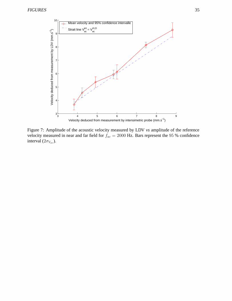
speaker. Figures 5, 6 and 7 show the acoustic velocity amplitude measured by LDV as a function

of the reference velocity amplitude forfac = 500 Hz, 1000 Hz and2000 Hz respectively. Each

velocity amplitude is obtained by averaging50 estimated values for the LDV and the reference

technique. Assuming that the statistical distribution of the acoustic velocity measured by LDV

is Gaussian, the bars represent the double of the standard deviationσVac(confidence interval at

95 %) of the50 measurements. The relative uncertainty in the acoustic velocity amplitude is

given by

uVac

Vac

=1

N

2σVac

Vac

, (14)

whereN is the number of measurement (50). The uncertainties are estimated to be±2% at500

Hz,±3% at1000 Hz and±2% at2000 Hz.

The bars representing the uncertainty in the reference velocity are lower than0.1 mm.s−1

which explains that they are not shown on the figures.




B Gazengel et al 15

Forfac = 500 Hz, the acoustic velcity amplitude measured by LDV and estimated by means

of the sound intensity probe agree. Forfac = 1000 Hz, the velocity amplitude measured with

LDV is near from the reference velocity. However, the variance in the LDV measured velocity

is greater than forfac = 500 Hz. Forfac = 2000 Hz, the acoustic velocity amplitude measured

by means of LDV is overestimated compared with the velocity deduced from the intensity

probe. The bias observed between the two curves can be explained by the bias due to the signal

processing (see section 2.2). Indeed, the signal processing leads to overestimate the acoustic

velocity amplitude, the bias observed between the two curves (reference velocity and measured

velocity) being the same order of magnitude than the bias observed in [26] due to the signal

processing. Morever, this difference may be explained by the fact that the two measurements

(LDV and reference) are not performed at the same point, the LDV probe being placed at a few

millimeters from the sound intensity probe.

5.1.2 Acoustic velocity phase measurement assessment

The phase difference between the acoustic velocity estimated by LDV and by the reference

technique (two microphone probe) are studied forfac = 500, 1000, 2000 Hz and in the near

and far field of the loudspeaker. The position of the probe on the loudspeaker axis are the same

as those used in the section 5.1.1. The phase characteristics (mean, variance) are estimated by

acquiring120 Doppler signal, each signal duration being1 second.

Results are the following. We obtain atfac = 500Hz a mean phase difference of10.31o

and a standard deviation of8.8o, at fac = 1000Hz a mean phase difference of17.7o and a

standard deviation of9.47o, atfac = 2000Hz a mean phase difference of1.57o and a standard

deviation of11.84o. These results show that it is possible to estimate a mean phase with a

B Gazengel et al 16

standard deviation less than20 degrees.

5.1.3 Discussion

The measurement of the acoustic velocity amplitude and phase with LDV can be performed in

free field using the Short Time Fourier Transform (STFT) for frequencies ranging from500 Hz

to 2000 Hz for acoustic velocity amplitudes greater than2 mm/s at500 Hz, 3 mm/s at1000 Hz,

4 mm/s at2000Hz corresponding to 92, 95.5 and 98 dB SPL in free field. The low frequency

limitation (500 Hz) is due to the flow velocity amplitude (smaller than50 mm/s) and to the

signal processing technique which requires that a single acoustic period is analysed during a

burst duration (see eq. 7). The amplitude limitation is due to the signal processing method,

which is adapted for high acoustic levels [26] corresponding to acoustic velocity amplitude

greater thani.fac (see equation 4).

5.2 Loudspeaker radiation model limits

This section presents the evaluation of the loudspeaker radiation model by comparing the on-

axis velocity measured by LDV and by the sound intensity probe with the on-axis velocity

calculated by means of the model described in appendix A. Theparameters used for the model

are estimated experimentally using the techniques described in appendix B and the acoustic

velocity is calculated using equation 15. The experiment isconducted forfac = 500 Hz in order

to be able to use the model presented in section 3 which assumes that the acoustic wavelenght

is much greater than the dimensions of the back cavity. The comparison of theoretical and

experimental pressure profile (see figure 11), shows that themodel is valid up tox = 10 cm.

After this limit, the experimental boundary conditions do not satisfy the hypothesis of the model.

B Gazengel et al 17

5.2.1 Far field radiation

The far field velocity pattern is presented in figure 8. Each point represents the mean value of50

estimations of acoustic velocity and the confidence interval at 95 % (2σVac) made by the LDV

probe, the sound intensity probe and the physical model.

As shown in the previous section, the acoustic velocity amplitude measured by means of

LDV and estimated by the sound intensity probe agree, the acoustic frequeny being low enough

for enabling precise estimations by means of LDV. The acoustic velocity amplitude estimated by

means of the propagation model has the same profile as this of the measured velocity. However,

a bias can be observed between the measured and the calculated velocity (about3 mm/s).

This bias is due to the error made in the physical parameters estimation which is based on a

model assuming a free field propagation whereas the far field propagation does not respect the

Sommerfeld condition because of the experimental conditions (finite dimension of the table

supporting the loudspeaker mounted in the baffle). This biascan be also observed on figure 11

giving the theoretical and experimental pressure profile.


5.2.2 Near field radiation


The near field velocity pattern is presented in figure 9. Each point represents the mean value

of 50 estimations of acoustic velocity and the confidence interval at 95 % (2σVac) made by the

LDV probe, the sound intensity probe and the physical model.The acoustic velocity amplitude

estimated by means of the propagation model is near from thismeasured by means of LDV, the

B Gazengel et al 18

bias being about1 mm/s. This bias is very low and confirms that the estimation ofradiation

model parameters (Ca andb0) is based on the analysis of pressure measured in the near field of

the loudspeaker as shown in appendix B. Figure 9 shows two different regions.

• For x < 10 cm, the acoustic level is high (110 dBSPL) and the frequency is low

(500 Hz), which enables to use LDV with confidence. The velocity measured by means

of LDV agrees with the theoretical velocity, the maximum bias being less than0.5 mm/s

(less than0.4 dB). This bias is also shown by figure 11 for the pressure profile. The ve-

locity estimated by means of the probe intensity differs from the theoretical one and from

the LDV measurement. The evanescent nature of the acoustic field in this region (near

field) may introduce many estimation errors of the velocity using the two microphone

method due to amplitude and phase mismatch [35, 33]. A more complete explanation of

this phenomenon would need a complementary study of the intensity probe located near

a sound source.

• Forx > 10 cm, the acoustic velocity amplitude measured by means of LDV and estimated

by the sound intensity probe agree, the bias being lower than0.5 dB. The bias observed

between the experimental and theoretical velocities is1mm/s (≃ 1 dB) as shown in

figure 11).

6 Conclusion

In this paper, the performances of a measuring LDV system areassessed for measuring acoustic

particle velocities in free field. In this context, the acoustic velocity is estimated by taking into

acccount the flow velocity due to natural convection. Once the frequency and amplitude range

B Gazengel et al 19

are determined, this system is used for characterizing the acoustic radiation of a loudspeaker.

In these experiments, the LDV bench is used in the back scattering configuration. The ve-

locity measured by means of LDV is estimated using three steps. At first, bursts are detected

with a threshold technique. This enables to estimate the beginning an ending time of each burst

and to derive the signal to noise ratio of the doppler signal for each burst. In a second step, the

instantaneous frequency of the doppler signal is estimatedusing a Short Time Frequency Trans-

form (STFT). Finally a post-processing is applied on the instantaneous frequency at different

times corresponding to the existence of bursts. This enables to estimate the velocity parameters

(acoustic amplitude and phase, flow velocity). The uncertainty in the acoustic velocity ampli-

tude and phase estimation is calculated using the standard deviation of 50 estimations of these

parameters. The reference velocity is estimated using a sound intensity probe put in the vicinity

of the probe volume. The uncertainty in the reference velocity are minimized using a relative

calibration of the probe.

Taking into account the constraints associated with the signal processing techniques, the

LDV bench is assessed in the [500 Hz - 2000 Hz] range. Results show that the LDV bench as-

sociated with the signal processing techniques described above enables to estimate the acoustic

velocity amplitude for500, 1000 Hz and2000 Hz for amplitude greater than2 mm/s. Differ-

ence observed between LDV measured velocity and reference velocity are the same order of

magnitude than these observed by numerical simulations formeasurement performed without

flow [26]. Concerning the acoustic velocity phase, the measurement of many bursts enables to

estimate the phase with a standard deviation less than20 degrees.

B Gazengel et al 20

The acoustic radiation of a loudspeaker is studied at 500 Hz using the LDV bench. The

acoustic velocity is calculated using a physical model and is measured by means of the LDV

probe and by means of a sound intensity probe. The parametersused in the physical model are

estimated by comparing the measured and calculated acoustic pressure on the axis of the loud-

speaker in the near field and far field. In the far field, resultsshow that the LDV probe and sound

intensity probe agree whereas the radiation model does not predict well the acoustic velocity.

This difference (about3 mm/s) is explained by the fact that the experimental conditions do not

respect the hypothesis used in the model. In the near field, the velocitiy amplitudes measured

by LDV, estimated by the sound intensity probe and calculated using the propagation model dif-

fer from about1 mm/s. The difference observed between the three velocity amplitudes (LDV,

sound intensity probe, model) in the far field are mainly explained by the bad estimation (due

to the experimental configuration) of the physical parameters used in the radiation model. The

difference observed in the near field are explained by the fact that the acoustic field is mainly

reactive in the near field of the loudspeaker. In this case, the amplitude and phase mismatch of

the two microphone can affect the acoustic velocity estimation [33].

These results show that it is possible to measure the acoustic velocity of a radiating struc-

ture in free field and encourage to characterize the near fieldacoustic radiation of a vibrating

structure, for which the flow velocity should be low due to viscous effect on the structure. The

accuracy of the LDV system should be increased by using a front scattering optical arrangement

or by using a more powerful laser beam in order to get a higher signal to noise ratio. The use

of other frequency demodulation technique should enable todecrease the minimum measurable

acoustic displacement,i.e., to decrease the minimum measurable acoustic velocity amplitude

B Gazengel et al 21

or to increase the maximum measurable acoustic frequency. The use of other detection process

should enable to increase the useful duration of burst (apparent length of the probe volume) and

then to decrease the minimum measurable frequency [36].

References

[1] C. G. Lomas.Fundamentals of Hot Wire Anemometry. Cambridge University Press, 1986.

[2] H. H. Bruun. Hot-Wire Anemometry, Principles and Signal Analysis. Oxford Science

Publications, 1995.

[3] H.E. de Bree. An overview of microflown technologies.Acta Acustica, 89:163–172, 2003.

[4] R. Lanoye, G. Vermeir, W. Lauriks, R. Kruse, and V. Mellert. Measuring the free field

acoustic impedance and absorption coefficient of sound absorbing materials with a com-

bined particle velocity-pressure sensor.J. Acous. Soc. Am., 119(5):2826–2831, 2006.

[5] F. Jacobsen and H. E. de Bree. A comparison of two different sound intensity measurement

principles.J. Acous. Soc. Am., 118(3):1510–1517, 2005.

[6] D.M. Campbell, J.A. Cosgrove, C.A. Greated, S.H. Jack, and D. Rockliff. Review of

LDA and PIV applied to the measurement of sound and acoustic streaming. Optics &

laser technology, 32(8):629–639, 2000.

[7] D.B. Hann and C.A. Greated. The measurement of flow velocity and acoustic particle

velocity using particle-image velocimetry.Meas. Sci. Tech., 8(12):1517–1522, 1997.

B Gazengel et al 22

[8] S. Moreau, R. Boucheron, J.C. Valiere, and H. Bailliet.Mesures LDV et PIV dans les

couches limites acoustiques. In9e Congres Francophone de Velocimetrie Laser, 2004.

Brussels, Belgium, september 2004.

[9] M. Michard, P. Blanc Benon, N. Grosjean, and C. Nicot. Apport de la vlocimtrie par im-

ages de particules pour la caractrisation duchamp de vitesse acoustique dans une maquette

de rfrigrateur thermoacoustique. In9e Congres Francophone de Velocimetrie Laser, 2004.

Brussels, Belgium, september 2004.

[10] H. Yeh and H.Z. Cummins. Localized fluid flow measurements with a He-Ne laser spec-

trometer.Appl. Phys. Lett., 4:176–178, 1964.

[11] K.J. Taylor. Absolute calibration of microphone by a laser-doppler technique.J. Acoust.

Soc. Am., 70(4):939–945, 1981.

[12] M.R. Davis and K.J. Hews Taylor. Laser doppler measurement of complex impedance.J.

Sound. Vib., 107(3):451–470, 1986.

[13] R. Raangs, T. Schlicke, and R. Barham. Calibration of a micromachined particle velocity

microphone in a standing wave tube using a lda photon-correlation technique.Meas. Sci.

Technol., 16:1099–1108, 2005.

[14] M. W. Thompson and A. A. Atchley. Simultaneous measurement of acoustic and stream-

ing velocities in a standing wave using laser doppler anemometry. J. Acoust. Soc. Am.,

117(4):1828–1838, 2005.

B Gazengel et al 23

[15] G. Lartigue, U. Meier, and C. Brat. Experimental and numerical investigation of self-

excited combustion oscillations in a scaled gas turbine combustor.Applied Thermal Engi-

neering, 24(11-12):1583–1592, 2004.

[16] J.C. Valiere, P. Herzog, V. Valeau, and G. Tournois. Acoustic velocity measurements in

the air by means of laser Doppler velocimetry : dynamic and frequency range limitations

and signal processing improvements.J. Sound and Vib., 229(3):607–626, 2000.

[17] C. Mellet, J.C. Valiere, and V. Valeau. Use of frequency trackers in laser doppler ve-

locimetry for sound field measurement : comparative study oftwo estimators.Mechanical

system and signal processing, 17(2):329–344, 2003.

[18] V. Valeau, J.C Valiere, and C. Mellet. Instantaneous frequency tracking of a sinusoidally

frequency-modulated signal with low modulation index: application to laser measure-

ments in acoustics.Signal Processing, 84(7):1147–1165, 2004.

[19] A. Le Duff, G. Plantier, J.C Valiere, and B. Gazengel. Acoustic velocity measurement in

weak flow by means of Laser Doppler Velocimetry : performanceof the Extended Kalman

Filter. J. Acous. Soc. Am., 2005. submitted.

[20] B. Gazengel, S. Poggi, and J.C. Valiere. Measurement of acoustic particle velocities in

enclosed sound field: Assessment of two laser doppler velocimetry measuring systems.

Applied Acoustics, 66(1):15–44, 2005.

[21] M.K. Mazumder, R.L. Overbey, and M.K. Testerman. Directional acoustic measurement

by laser doppler velocimeters.Applied Physics Letters, 29(7):416–418, 1976.

[22] C.A Greated. Measurement of acoustic velocity fields.Strain, 22:21–24, 1986.

B Gazengel et al 24

[23] G. Souchon, B. Gazengel, O. Richoux, and A. Le Duff. Characterization of dipole radi-

ation by laser doppler velocimetry. In7eme Congres Francais d’Acoustique, CFA, Stras-

bourg, 22-25 Mars 2004.

[24] H. E. Albrecht, N. Damaschke, M. Borys, and C. Tropea.Laser Doppler and Phase

Doppler Measurement Techniques. Springer Verlag, 2003.

[25] A. Degroot, O. Richoux, and L. Simon. Joint measurementof particle acoustic velocity

and flow velocity by means of laser Doppler velocimetry (LDV). In Actes du PSIP’2005,

pages 295–300, Toulouse, 31 janvier-2 fvrier 2005.

[26] B. Gazengel, S. Poggi, and J.C. Valiere. Evaluation ofthe performance of two acquisition

and signal processing systems for measuring acoustic particle velocities in air by means

of laser doppler velocimetry.Meas. Sci. Technol., 14(12):2047–2064., 2003.

[27] P. Rouquier, B. Gazengel, O. Richoux, L. Simon, G. Tournois, and M. Bruneau. Acoustic

particle velocities measurement by means of laser doppler velocimetry : application to

harmonic acoustic field in free space with weak flow. InProceedings of Forum Acusticum,

Seville, 16-20 septembre 2002.

[28] P. Rouquier.Mesure de vitesses particulaires acoustiques en champ libre par Vlocimtrie

Laser Doppler : dveloppement du banc de mesure et valuation des performances. PhD

thesis, Universite du Maine, Le Mans, septembre 2004.

[29] L. Simon, O. Richoux, A. Degroot, and L. Lionet. Laser doppler velocimetry joint mea-

surements of acoustic and mean flow components : Lms-based algorithm and crb calcula-

tions. submitted, 2006.

B Gazengel et al 25

[30] J. Zemanek. Beam behavior within the nearfield of a vibrating piston.J. Acoust. Soc. Am.,

49(1B):181–191, 1970.

[31] E. Geddes. Source radiation characteristics.J. Audio. Eng. Soc., 34(6):464–478, 1986.

[32] J.C. Pascal and C. Carles. Systematic measurement errors with two microphone sound

intensity meters.J. Sound Vib., 83(1):53–65, 1982.

[33] F. Jacobsen. A note on finite difference estimation of acoustic particle velocity.J. Sound.

Vib., 256(5):849–859, 2002.

[34] G. Gouesbet. On the scattering of light by a mie scatter center located on the axis of an

axisymmetric light profile.J. Opt., 13:97–103, 1982.

[35] G.C. Steyer, R. Singh, and D.R. Houser. Alternative spectral formulations for acoustic

velocity measurement.J. Acoust. Soc. Am., 81(6):1955–1961, 1987.

[36] A. Degroot, S. Montresor, B. Gazengel, O. Richoux, and L. Simon. Doppler signal de-

tection and particle time of flight estimation using wavelettransform for acoustic velocity

measurement. InICASSP, Toulouse, France, May 14-19 2006.

[37] J.C. Le Roux.Le haut-parleur lectrodynamique : estimation des paramtres lectroacous-

tiques aux basses frquences et modlisation de la suspension. PhD thesis, Universite du

Maine, Le Mans, avril 1994.

B Gazengel et al 26

A On-axis acoustic velocity

Considering that the loudspeaker is mounted in an infinite baffle and that it radiates in a half

space, the radiated field at position~r (in (x,y) frame) is calculated using the Rayleigh integral

p(~r) =jkρc

2πVp

∫

Sp

e−jk|~r−~r0|

|~r − ~r0|dS0, (15)

whereSp is the surface of the piston,Vp is the piston velocity,k = ωac/c = 2πfac/c is the

wavenumber,ρ is the air density andc is the sound speed.~r0 is the position of an elementary

source of the piston in the piston reference frame anddS0 is the surface of the elementary

source. For a circular piston of radiusRp, the pressure along the piston axis is

p(x) = ρcVpe−jkx(1 − e−jk

√x2+R2

p−x). (16)

Using the Euler equation, the velocity along the piston axisis

v(x) = Vpe−jkx(1 − x

√

x2 + R2p

e−jk√

x2+R2p−x). (17)

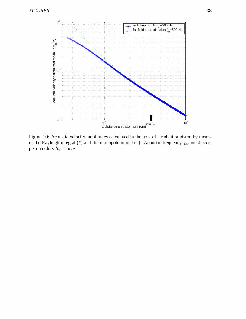
The far field approximation (given byRp << x) leads to the expression of the far field acoustic

velocity

vff (x) =1 + jkx

2π

Qp

x2e−jkx, (18)

whereQp = πR2pVp is the acoustic volume velocity of the loudspeaker. Equation 18 gives the

expression of the acoustic velocity due to a monopole of volume velocityQp. The comparison

of the equations 9 and 18 enables to define the near field of the loudspeaker. Figure 11 shows

the two velocty profiles forfac = 500Hz andRp = 5cm (see section B). The near field of the

loudspeaker is arbitrarily defined when the two velocity amplitudes differ from1%. This leads

in this particular case to a near field limitdff = 37cm in this case.


B Gazengel et al 27

B Radiation model parameters estimation

The equivalent piston radiusRp is estimated by measuring the diameter of the suspension as

proposed by Le Roux [37].

In order to estimate the velocity of the pistonVp used in the propagation model, the volume

velocity generated by the loudspeaker is measured. This is done by using a closed cavity at the

back of the loudspeaker. Assuming that there is no leakage, the volume velocity generated by

the loudspeakerQp is deduced from the pressure measured inside the cavitypc, for a harmonic

excitation at angular frequencyωac, by

Qp = jωacCapc, (19)

whereCa is the acoustic compliance of the back cavity. The estimation of the membrane surface

Sp using the measured radiusRp enables to deduce the membrane mean velocity.

The value of the acoustic complianceCa of the back cavity is estimated by measuring the

acoustic pressure amplitude profile along the loudpseaker axis given by

∣

∣

∣

∣

∣

p(x)

pc

∣

∣

∣

∣

∣

2

= 2

(

ωacρcCa

Sp

)2[

1 − cos[

k(√

(x − xp)2 + R2p − (x − xp))

]]

(20)

Using the measured acoustic pressure on the loudpseaker axis, a least square method enables to

estimate the two parametersCa andxp [28]. The experimental and calculated pressure pattern

are presented in figure 11. This shows that the values of parametersCa andxp enable to predict

well the very near field pressure (x < 10cm).


B Gazengel et al 28

List of Figures

1 Optical set-up of the LDV system. The probe volume is ellipsoidal and containsfringes. Particles are represented by black circles. Arrows represent the particlevelocities. . . . . . . . . . . . . . . . . . . . . . . . . . . . . . . . . . . . . . 29

2 General principle of the signal processing for acoustic velocity estimation. . . . . . . 303 Schematic view of the loudspeaker.xp is the abscissa of the equivalent piston

in the loudspeaker reference frame (x0, y0). . . . . . . . . . . . . . . . . . . . 314 Schematic view of the experimental system . . . . . . . . . . . . . .. . . . . 325 Amplitude of the acoustic velocity measured by LDVvsamplitude of the refer-

ence velocity measured in near and far field forfac = 500 Hz. Bars representthe95 % confidence interval (2σVac

). . . . . . . . . . . . . . . . . . . . . . . . 336 Amplitude of the acoustic velocity measured by LDVvsamplitude of the refer-


). . . . . . . . . . . . . . . . . . . . . . . . 347 Amplitude of the acoustic velocity measured by LDVvsamplitude of the refer-


). . . . . . . . . . . . . . . . . . . . . . . . 358 Far field acoustic velocity amplitude as a function of distancex from the loud-

speaker forfac = 500 Hz. LDV measurement (star), probe measurement(square), model (circle). . . . . . . . . . . . . . . . . . . . . . . . . . . . .. . 36

9 Near field acoustic velocity amplitude as a function of distancex from the loud-speaker forfac = 500 Hz. LDV measurement (*), probe measurement (), model(o). . . . . . . . . . . . . . . . . . . . . . . . . . . . . . . . . . . . . . . . . . 37

10 Acoustic velocity amplitudes calculated in the axis of a radiating piston bymeans of the Rayleigh integral (*) and the monopole model (-.). Acoustic fre-quencyfac = 500Hz, piston radiusRp = 5cm. . . . . . . . . . . . . . . . . . 38

11 Acoustic pressure amplitudes in the axis of a radiating piston. Acoustic fre-quencyfac = 500Hz, piston radiusRp = 5cm. x : experimental. - : calculated. 39

FIGURES 29

��

x

yz

PM

emitting

receivingoptics

Beamsplitter

1W Argon laser

optics

cell

Bragg

θ

dx

Figure 1: Optical set-up of the LDV system. The probe volume is ellipsoidal and containsfringes. Particles are represented by black circles. Arrows represent the particle velocities.

FIGURES 30

DetectionEstimationValidation

Frequency

Demodulation

(sinusoïdal)Excitation signal

System under

investigation

Instantaneous

measuredLDV system

Central time

Excitation frequency

Doppler signal

Time of flight

Frequency

Velocity to be

Threshold

SNR

estimationParametric

Vac φac Vf,q

Figure 2:General principle of the signal processing for acoustic velocity estimation.

FIGURES 31

px

y0

x0

Equivalent piston

Reference frame

y

x

Figure 3: Schematic view of the loudspeaker.xp is the abscissa of the equivalent piston in theloudspeaker reference frame (x0, y0).

FIGURES 32

Probe volume

Loudspeaker axis

RearMicrophone

Screen

Rear cavity

IntensimØtric probe

��

��

Emitting optics

Receiving optics

Laser beams

Loudspeaker

x~ex

Figure 4: Schematic view of the experimental system

FIGURES 33

1 2 3 4 5 6 7 8 9 101

2

3

4

5

6

7

8

9

10

Velocity deduced from measurement by intensimetric probe (mm.s−1)

Vel

ocity

ded

uced

from

mea

sure

men

t by

LDV

(m

m.s

−1 )

Mean velocity and 95% confidence intervalle Strait line V

acint = V

acVLD

Figure 5: Amplitude of the acoustic velocity measured by LDVvsamplitude of the referencevelocity measured in near and far field forfac = 500 Hz. Bars represent the95 % confidenceinterval (2σVac

).

FIGURES 34

3 3.5 4 4.5 5 5.5 6 6.5 7 7.5 82

3

4

5

6

7

8

9

10


Vel

ocity

ded

uced

from

mea

sure

men

t by

LDV

(m

m.s

−1 )


acint = V

acVLD


).

FIGURES 35

3 4 5 6 7 8 93

4

5

6

7

8

9

10


Vel

ocity

ded

uced

from

mea

sure

men

t by

LDV

(m

m.s

−1 )


acint = V

acVLD


).

FIGURES 36

30 40 50 60 70 80 90 1000

2

4

6

8

10

12

14

Measurement point position x0 (cm)

Aco

ustic

par

ticle

vel

ocity

(m

m.s

−1 )

LDV velocityModel velocityProbe velocity

Figure 8: Far field acoustic velocity amplitude as a functionof distancex from the loudspeakerfor fac = 500 Hz. LDV measurement (star), probe measurement (square), model (circle).

FIGURES 37

8 9 10 11 12 13 14 15 16 174

6

8

10

12

14

16

Measurement point position x0 (cm)

Aco

ustic

par

ticle

vel

ocity

(m

m.s

−1 )

LDV velocityModel velocityProbe velocity

Figure 9: Near field acoustic velocity amplitude as a function of distancex from the loudspeakerfor fac = 500 Hz. LDV measurement (*), probe measurement (), model (o).

FIGURES 38

10−1

100

10−2

10−1

100

Aco

ustic

vel

ocity

nor

mal

ized

mod

ulus

vac

(z)

x distance on piston axis (cm)37,5 cm

radiation profile fac

=500 Hzfar field approximation f

ac=500 Hz

Figure 10: Acoustic velocity amplitudes calculated in the axis of a radiating piston by meansof the Rayleigh integral (*) and the monopole model (-.). Acoustic frequencyfac = 500Hz,piston radiusRp = 5cm.

FIGURES 39

10−3

10−2

10−1

100

10−4

10−3

10−2

10−1

100

20 cmx0 distance (m)

Pre

ssur

e p ac

on

pres

sure

par

rat

io

Theoretical profileExperimental profile

Figure 11: Acoustic pressure amplitudes in the axis of a radiating piston. Acoustic frequencyfac = 500Hz, piston radiusRp = 5cm. x : experimental. - : calculated.

characterization of a loudspeaker free ï¬eld radiation by

Documents