characterization of airflow through an air …
TRANSCRIPT

CHARACTERIZATION OF AIRFLOW THROUGH AN AIR HANDLING UNIT
USING COMPUTATIONAL FLUID DYNAMICS
by
Andrew Evan Byl
A thesis submitted in partial fulfillment
of the requirements for the degree
of
Master of Science
In
Mechanical Engineering
MONTANA STATE UNIVERSITY
Bozeman, Montana
November 2015

©COPYRIGHT
by
Andrew Evan Byl
2015
All Rights Reserved
ii
TABLE OF CONTENTS
1. INTRODUCTION ...........................................................................................................1
2. BACKGROUND .............................................................................................................5
HVAC Systems .............................................................................................................. 5
Air Filters ................................................................................................................ 6
Flow Conditioners and Baffles ............................................................................... 7
Fan Types ................................................................................................................ 8
Heat Exchangers ................................................................................................... 12
Computational Fluid Dynamics ................................................................................... 15
CFD in the HVAC Industry .................................................................................. 17
Methods of Characterizing Flow .................................................................................. 21
Flow Visualization ................................................................................................ 21
Numerical Methods for Characterizing Flow ....................................................... 24
3. EXPERIMENTAL PROCEDURE ................................................................................28
Straight Duct ................................................................................................................ 29
Test Setup.............................................................................................................. 29
Full AHU ...................................................................................................................... 31
Test Setup.............................................................................................................. 31
Baffles .......................................................................................................................... 32
4. COMPUTATIONAL FLUID DYNAMICS METHODOLOGY ..................................34
Computational Fluid Dynamics Models ...................................................................... 34
Heating and Cooling Coils .................................................................................... 35
Full AHU .............................................................................................................. 37
Simplified AHU .................................................................................................... 38
Baffle Design ........................................................................................................ 41
Meshing ........................................................................................................................ 42
CFD Flow Characterization ......................................................................................... 44
5. RESULTS ......................................................................................................................51
Straight Duct ................................................................................................................ 51
Full AHU ...................................................................................................................... 53
Base AHU ............................................................................................................. 53

iii
TABLE OF CONTENTS – CONTINUED
AHU with Wing Baffle ......................................................................................... 56
Full Versus Simplified AHU ........................................................................................ 60
Base AHU ............................................................................................................. 61
AHU with Wing Baffle ......................................................................................... 67
Simplified AHU ........................................................................................................... 72
Assessing Performance ................................................................................................ 74
Flow Characteristics.............................................................................................. 74
Heating Coil .......................................................................................................... 83
6. CONCLUSION ..............................................................................................................90
REFERENCES CITED ......................................................................................................94

iv
LIST OF TABLES
Table Page
5.1: Uniformity and Turbulence Values for Plane 1, 1000 RPM ......................... 76
5.2: Uniformity and Turbulence Values for Plane 2, 1000 RPM ......................... 76
5.3: Uniformity and Turbulence Values for Plane 3, 1000 RPM ......................... 76
5.4: Uniformity and Turbulence Values for Plane 1, 1800 RPM ......................... 78
5.5: Uniformity and Turbulence Values for Plane 2, 1800 RPM ......................... 78
5.6: Uniformity and Turbulence Values for Plane 3, 1800 RPM ......................... 78
5.7: Vorticity Values for Plane 1, 1000 RPM ....................................................... 80
5.8: Vorticity Values for Plane 2, 1000 RPM ....................................................... 81
5.9: Vorticity Values for Plane 3, 1000 RPM ....................................................... 81
5.10: Vorticity Values for Plane 1, 1800 RPM ..................................................... 82
5.11: Vorticity Values for Plane 2, 1800 RPM ..................................................... 82
5.12: Vorticity Values for Plane 3, 1800 RPM ..................................................... 82
5.13: Heat transfer rate with pressure resistance coefficients ............................... 84
5.14: Heat transfer rate, no pressure resistance coefficients ................................. 84
5.15: Uniformity and turbulence values for Plane 1, 1000 RPM .......................... 86
5.16: Uniformity and turbulence values for Plane 2, 1000 RPM .......................... 86
5.17: Uniformity and turbulence values for Plane 3, 1000 RPM .......................... 86
5.18: Uniformity and turbulence values for Plane 1, 1800 RPM .......................... 86
5.19: Uniformity and turbulence values for Plane 2, 1800 RPM .......................... 87
5.20: Uniformity and turbulence values for Plane 3, 1800 RPM .......................... 87
5.21: Vorticity values for Plane 1, 1000 RPM ...................................................... 88

v
LIST OF TABLES – CONTINUED
Table Page
5.22: Vorticity values for Plane 2, 1000 RPM ...................................................... 88
5.23: Vorticity values for Plane 3, 1000 RPM ...................................................... 88
5.24: Vorticity values for Plane 1, 1800 RPM ...................................................... 88
5.25: Vorticity values for Plane 2, 1800 RPM ...................................................... 89
5.26: Vorticity values for Plane 3, 1800 RPM ...................................................... 89
vi
LIST OF FIGURES
Figure Page
2.1: Diagram of an air conditioning system [15] .................................................... 6
2.2: Axial flow fan wheel (left) and airflow direction (right) ............................... 10
2.3: Centrifugal fan impeller wheel (left) and airflow direction (right) [23] ........ 10
2.4: Forward curved vs backward curved centrifugal fan blade designs [23] ...... 11
2.5: Fan housing .................................................................................................... 12
2.6: Rotary wheel heat exchanger [24] ................................................................. 13
2.7: A fin tube heat exchanger [25] ...................................................................... 14
2.8: Contours as a visual representation (velocity magnitude) ............................. 23
2.9: Vectors as a visual representation (velocity on a plane) ................................ 23
2.10: Streamlines as a visual representation (colored to velocity magnitude) ...... 24
2.11: Isosurface as a visual, velocity range 2-3 m/s ............................................. 24
3.1: Straight duct experiment ................................................................................ 30
3.2: AAON V3-A Air Handling Unit ................................................................... 32
3.3: Wing baffle used in experiments ................................................................... 33
3.4: Wing baffle location ...................................................................................... 33
4.1: Full AHU model with regions ....................................................................... 38
4.2: Simplified AHU with heating coil region ...................................................... 40
4.3: Location of Planes 1, 2, and 3 and Lines 1, and 2 ......................................... 40
4.4: First perforated plate: uniform hole pattern using 0.025 m diameter holes ... 42
4.5: Second perforated plate. ................................................................................ 42
5.1: Simulated vs experimental pressure drop data for the cooling coil ............... 52

vii
LIST OF FIGURES – CONTINUED
Figure Page
5.2: Base AHU 1000 RPM experimental vs simulated velocity
data from Line 1 ............................................................................................ 54
5.3: Base AHU 1000 RPM experimental vs simulated velocity
data from Line 2 ............................................................................................ 55
5.4: Base AHU 1800 RPM experimental vs simulated velocity
data from Line 1 ............................................................................................ 55
5.5: Base AHU 1800 RPM experimental vs simulated velocity
data from Line 2 ............................................................................................ 56
5.6: AHU with wing baffle, 1000 RPM experimental vs simulated
velocity data from Line 1 .............................................................................. 58
5.7: AHU with wing baffle, 1000 RPM experimental vs simulated
velocity data from Line 2 .............................................................................. 58
5.8: AHU with wing baffle, 1800 RPM experimental vs simulated
velocity data from Line 1 .............................................................................. 59
5.9: AHU with wing baffle, 1800 RPM experimental vs simulated
velocity data from Line 2 .............................................................................. 59
5.10: Velocity and linear regression values on Plane 2 for the
full AHU model, 1000 RPM. ....................................................................... 61
5.11: Contour plots from Plane 1 of the full AHU model, 1000 RPM ................. 62
5.12: Contour plots from Plane 1 of the transient simplified
AHU model, 1000 RPM .............................................................................. 63
5.13: Contour plots from Plane 1 of the steady-state simplified
AHU model, 1000 RPM .............................................................................. 63
5.14: Contour plots from Plane 2 of the full AHU model, 1000 RPM ................. 63
5.15: Contour plots from Plane 2 of the transient simplified
AHU model, 1000 RPM .............................................................................. 63
5.16: Contour plots from Plane 2 of the steady-state simplified
AHU model, 1000 RPM .............................................................................. 64

viii
LIST OF FIGURES – CONTINUED
Figure Page
5.17: Contour plots from Plane 3 of the full AHU model, 1000 RPM ................. 64
5.18: Contour plots from Plane 3 of the transient simplified
AHU model, 1000 RPM .............................................................................. 64
5.19: Contour plots from Plane 3 of the steady-state simplified
AHU model, 1000 RPM .............................................................................. 64
5.20: Contour plots from Plane 1 of the full AHU model, 1800 RPM ................. 65
5.21: Contour plots from Plane 1 of the transient simplified
AHU model, 1800 RPM .............................................................................. 65
5.22: Contour plots from Plane 1 of the steady-state simplified
AHU model, 1800 RPM .............................................................................. 65
5.23: Contour plots from Plane 2 of the full AHU model, 1800 RPM. ................ 65
5.24: Contour plots from Plane 2 of the transient simplified
AHU model, 1800 RPM .............................................................................. 66
5.25: Contour plots from Plane 2 of the steady-state simplified
AHU model, 1800 RPM .............................................................................. 66
5.26: Contour plots from Plane 3 of the full AHU model, 1800 RPM ................. 66
5.27: Contour plots from Plane 3 of the transient simplified
AHU model, 1800 RPM .............................................................................. 66
5.28: Contour plots from Plane 3 of the steady-state simplified
AHU model, 1800 RPM .............................................................................. 67
5.29: Contour plots from Plane 1 of the full wing baffle model, 1000 RPM ....... 67
5.30: Contour plots from Plane 1 of the transient simplified
wing baffle model, 1000 RPM ..................................................................... 68
5.31: Contour plots from Plane 1 of the steady-state simplified
wing baffle model, 1000 RPM ..................................................................... 68
5.32: Contour plots from Plane 2 of the full wing baffle model, 1000 RPM ....... 68
ix
LIST OF FIGURES – CONTINUED
Figure Page
5.33: Contour plots from Plane 2 of the transient simplified
wing baffle model, 1000 RPM ..................................................................... 68
5.34: Contour plots from Plane 2 of the steady-state simplified
wing baffle model, 1000 RPM ..................................................................... 69
5.35: Contour plots from Plane 3 of the full wing baffle model, 1000 RPM ....... 69
5.36: Contour plots from Plane 3 of the transient simplified
wing baffle model, 1000 RPM ..................................................................... 69
5.37: Contour plots from Plane 3 of the steady-state simplified
wing baffle model, 1000 RPM ..................................................................... 69
5.38: Contour plots from Plane 1 of the full wing baffle model, 1800 RPM ....... 70
5.39: Contour plots from Plane 1 of the transient simplified
wing baffle model, 1800 RPM ..................................................................... 70
5.40: Contour plots from Plane 1 of the steady-state simplified
wing baffle model, 1800 RPM ..................................................................... 70
5.41: Contour plots from Plane 2 of the full wing baffle model, 1800 RPM ....... 70
5.42: Contour plots from Plane 2 of the transient simplified
wing baffle model, 1800 RPM ..................................................................... 71
5.43: Contour plots from Plane 2 of the steady-state simplified
wing baffle model, 1800 RPM ..................................................................... 71
5.44: Contour plots from Plane 3 of the full wing baffle model, 1800 RPM ....... 71
5.45: Contour plots from Plane 3 of the transient simplified
wing baffle model, 1800 RPM ..................................................................... 71
5.46: Contour plots from Plane 3 of the steady-state simplified
wing baffle model, 1800 RPM ..................................................................... 72
5.47: Streamlines for a) base AHU model b) wing baffle model, 1000 RPM ...... 73
5.48: Streamlines for AHU model, 1000 RPM with
a) perforated plate 1 b) perforated plate 2 ................................................... 73

x
ABSTRACT
HVAC equipment manufacturers spend a considerable amount of time and effort
updating existing product lines in order to meet the ever-increasing demand for energy
efficient systems. As a major part of HVAC systems, an air handling unit (AHU) controls
the airflow through the system and regulates the indoor air quality. Plenum fans used in
AHUs inherently produce a rotational airflow, which can create highly unstructured airflow
as it enters a heat exchanger located downstream. This in turn leads to lower heat transfer
rates and premature heat exchanger failure. As such, airflow uniformity is presently
regarded as an important consideration in designing these systems. Through advancements
in computer technologies within the last decade, computational fluid dynamics (CFD) has
become an economical solution allowing HVAC equipment designers to numerically
model prototypes and reduce the time required to optimize a given design and identify
potential failure points. While CFD analysis also offers the ability to visualize and
characterize the airflow through an AHU system, it has often been used to model individual
components such as fans or heat exchangers without analyzing them as a single unit. This
work presents the CFD models used to characterize the airflow within an AHU in order to
aid in understanding the effects that flow uniformity has on heat exchanger performance.
The airflow uniformity was analyzed over a range of volumetric flow rates, and
experiments were used to validate the baseline simulations. Different baffle designs were
then added into the validated simulations to observe their influence on both airflow
uniformity and heat transfer performance. Results indicate that airflow uniformity is, by
itself, an insufficient metric to predict heat transfer performance. Additionally, steady-state
CFD analyses performed on simplified geometries are shown to provide a sufficient model
to be used for further optimization, when the inlet conditions are well specified.
1
1 INTRODUCTION
For most buildings around the world, the heating, ventilation, and air conditioning
(HVAC) systems consume a large amount energy. 47% of the total energy usage in
residential buildings was used towards heating and air conditioning in 2009 [1].
Furthermore, in 2014 41% of the total U.S. energy consumption was consumed in both
residential and commercial buildings [2]. As a major part of these systems, air handling
units (AHU) are used to distribute conditioned air to spaces within a building to improve
indoor air quality. In a time now where energy efficiency and sustainability is becoming a
must, the efficiency of these units have become highly important. Of all the factors that can
contribute to unit efficiency, one that has not gathered much attention is the effect that
airflow quality has on the overall performance of an AHU system.
HVAC technologies provide a comfortable indoor living environment around the
world. Of the three types of processes included in HVAC, ventilation is perhaps the most
important one as far as indoor air quality goes. Proper ventilation allows the removal of
airborne particulates such as bacteria, dust, and smoke to provide clean air to indoor
habitants. It also controls the humidity as well as the volume of air that gets recirculated
through a building. The method of ventilation most commonly used is through
mechanically forcing the air via an air handling unit. AHUs are made up of a number of
individual components, with the most basic designs being connected to ventilation ducting
and consisting of a fan unit to move air, and heating and/or cooling elements to condition
it. Each of these components have a number of efficiencies, which contributes to the
effectiveness of the whole system. These efficiencies can include that of the fan motor, the

2
loss from a belt drive, the fan design, the heat transfer properties of heat exchangers, and
the uniformity of the air flow downstream of the fan. Looking closer at the latter of these,
research has found that non-uniform airflow across a heat exchanger can have a substantial
effect, causing the average heat transfer coefficient to drop [3]. This non-uniform flow
comes from the centrifugal effects of the fan itself [4], and due to the drop in the heat
transfer coefficient, more air must be drawn across a heat exchange to transfer the same
amount of heat as would be required with a uniform flow.
In the past, the design and optimization progression for air handling units has been
that of an iterative process, involving the physical construction and testing of a complete
system. This method of optimization does work; however, it is time consuming and costly,
requiring new components, and potentially a full unit from scratch, to be built and tested
for each iteration. Furthermore, the experimental flow field measurements used to indicate
a complex flow generally lack the detail to provide a larger-scale picture.
Flow visualization is a technique that is able to minimally provide a depiction of
the large scale flow patterns, which can indicate areas of flow recirculation, flow separation
caused by the fluid interactions with the fan, and any potential obstructions in the flow
path. Advanced visualization techniques can be leveraged to provide quantitative
assessments of the flow. One such method of flow visualization is particle image
velocimetry (PIV), which uses lasers to track particles which have been injected into the
flow. PIV has been used in the past to measure the air velocity profiles across finned-tube
heat exchangers [5], and to measure an indoor airflow field [6]. However, this technique
can greatly add to the cost of testing depending on the accuracy of the equipment used, and

3
does not eliminate the need to build a physical model for each test.
Alternatively, the use of computational fluid dynamics (CFD) can be a powerful
tool in this application space as it allows the designer to model multiple iterations at a time,
visually see airflow patterns, and provide definitive numbers of flow rate, heat transfer,
turbulence, etc. without requiring a physical prototype for each simulation. The HVAC
industry has recently started using CFD analysis with increasing frequency, which has
already proven to be a valuable tool in other fields [7, 8, 9]. In the past, it had been primarily
used as a secondary check after the primary design has been built, but has since moved into
one of the principal steps in the design process. Over the last decade, within the HVAC
industry, there has been a number of research projects involving CFD analysis, with topics
ranging from the airflow in a hospital operating room [10] and data centers [11] to the flow
across a heat exchanger [12] or through a fan [13]. The main motivation of this previous
research has been to characterize airflow within individual components, such as ventilation
ducting, centrifugal fans, and heating and cooling coils. The focus on these projects,
though, has been mainly to illustrate a picture of the airflow as a reference, rather than as
a simultaneous part of the design process. This limited use of CFD analysis in the HVAC
industry means that many manufacturers still either spend substantial time and money
physically testing these units, or they opt not to redesign them at all.
The purpose of this research is to 1) effectively characterize the airflow patterns
occurring in a prototype air handling unit manufactured by AAON, Inc. using CFD
analysis, and 2) to insert different baffle designs into the system and illustrate the effect
each has on the downstream flow regime. An air handler unit was modeled using 3D CAD

4
techniques, then imported into the commercially available CFD code, Star-CCM+®, to
characterize the uniformity in the air flow across a heating exchanger section. This model
was then validated using experimental data, and different baffle designs were incorporated
into the model. The effects due to these baffles were then analyzed using CFD to observe
the predicted flow patterns.
5
2 BACKGROUND
This section introduces the use of computational fluid dynamics, focusing on the
HVAC industry. Firstly, air handling units and the components they are made up of are
discussed. Secondly, the methods for physically and numerically characterizing fluid flow
are considered. Finally, a brief history of computational fluid dynamics (CFD) and its role
in the HVAC industry is examined.
HVAC Systems
HVAC refers to the technology that controls the indoor environment with a goal to
provide thermal comfort and acceptable indoor air quality for residential, commercial, and
industrial buildings [14]. These systems vary greatly in size, shape, and number of
components depending on the intended application. As a major element of an HVAC
system, an AHU is designed to meet a variety of objectives, which includes providing air
movement, ventilation to allow fresh air to enter the system, cleaning the air,
humidification or dehumidification, and the heating or cooling of the air through the
system. An AHU generally consists of a number of components to complete these
objectives, such as a fan, filter, humidifier, heating coil, and a cooling coil. An example
configuration of an AHU can be seen in Figure 2.1. Each of these components affects the
airflow in some way. How the components change the airflow relates back not only to the
overall efficiency of each individual component. For example, the pressure drop created
by one of these components causes a resistance for the air to flow, which then requires the
fan to use more energy to achieve the same flow rate as before. This in turn increases the

6
power consumption of the AHU and negatively impacts the maintenance cost of the fan
unit.
Figure 2.1: Diagram of an air conditioning system [15]
Air Filters
The average American spends approximately 90% their day inside environments
such as a building or vehicle [16]. These environments contain particulates, where the
health of occupants is related to particulate concentration [17]. Air filters are used in HVAC
systems to remove these particulates from the air before it is circulated through the
building. These filters are placed upstream of the evaporator coil, and can be placed in
strategic slots in the ducting system depending on indoor air quality requirements. The
filters remove particulates by trapping them within the filter material which has pores that
are slightly larger than the largest particle that is allowed to pass, thus allowing air and only
the smallest particles to pass through. As the filter collects more particulates, it becomes
increasingly dense and more efficient at blocking additional objects. This also increases

7
the resistance, reducing the airflow and causing the fan to experience more static energy.
Furthermore, if the filter becomes too full of particles, it can become a source of air
pollution. Removing the filter can solve these problems, but would allow the particles up
on other components, such as the cooling coil, which would eventually cause it to fail [18].
High-Efficiency Particulate Air (HEPA) filters and Electrostatic precipitators (ESPs) are
commonly used to filter airflow in an AHU. HEPA filters are a pleated filter type that needs
to be replaced periodically as they can eventually contribute to air pollution instead of
preventing it. ESPs use an electric field to collect particulates instead of material stretched
across the duct, which greatly reduces the pressure drop compared to traditional filters, but
it also has a low collection efficiency [19].
Flow Conditioners and Baffles
A fully developed flow is where the velocity profile does not change within in the
fluid flow direction. Flow meters are used to measure fully-developed flow through a pipe
or duct of a manufacturer specified length. However, the length of ducting required to reach
a fully developed flow is rarely achievable in industry. Flow conditioners are normally
used to reduce any disturbances that may be present in the flow that can result from fans,
elbows, valves, and expansions within the system. This allows a shorter duct or pipe run to
be used to achieve a fully-developed flow. Different flow conditioners exist that can be
used to help develop the flow. Research has been performed comparing the performance
of many of these designs [20, 21, 22]. Many of these conditioners are evolved forms of
honeycomb, vanes, and screens used in early wind tunnel test research. Tube bundles and
perforated plates are ruggedized versions of honeycombs and screens. These types

8
generally remove swirling and reduce turbulence levels. While good at removing flow
distortions, they are limited by the total static pressure drop added to the system. The tab-
type conditioner actually increases a fluid’s turbulence level by creating vortices in the
flow. This accelerates the swirl reduction and velocity profile correction that occurs
naturally in longer straight-pipe lengths. Tab-conditioners generally cause a low pressure
drop and are not as susceptible to fouling as many other kinds are, and hence require less
maintenance to clean. The main limitation with using tab-conditioners is that they are not
well suited for flows that have a Reynolds number of less than 20,000 [20]. As the Reynolds
number can be greatly influenced by the individual geometries and range of flow rates in
an HVAC system, tab-conditioners should be considered on a case-by-case basis.
Baffles and diffusers are another tool to control airflow within an AHU. While flow
conditioners generally decrease swirling and turbulence in a fluid in order to straighten the
flow, baffles and diffusers are designed to enhance mixing. The simplest form of a baffle
is a straight metal plate which is oriented in a manner that redirects the airflow in a desired
direction. This same baffle can also be used to control the amount of airflow entering a
system, such as with an outside air damper for an AHU.
Fan Types
There are several different design characteristics of fans that can be utilized in an
AHU. Some can include the fan drive-train, mounting style and orientation, fan blade
design, and whether the fan is encased. Performance curves show the RPM, static pressure,
power, and efficiency for various flow rates of any fan. For a given fan, the static pressure
required to move a certain flow through is characterized by the system curve. Most often
9
for a specific fan geometry, designers will only test a few sizes at preset speeds instead of
an evaluation of each fan at ever operating condition. The data from these tests is used to
calculate fan curve values at specific points. In order to find the rest of the curve, the
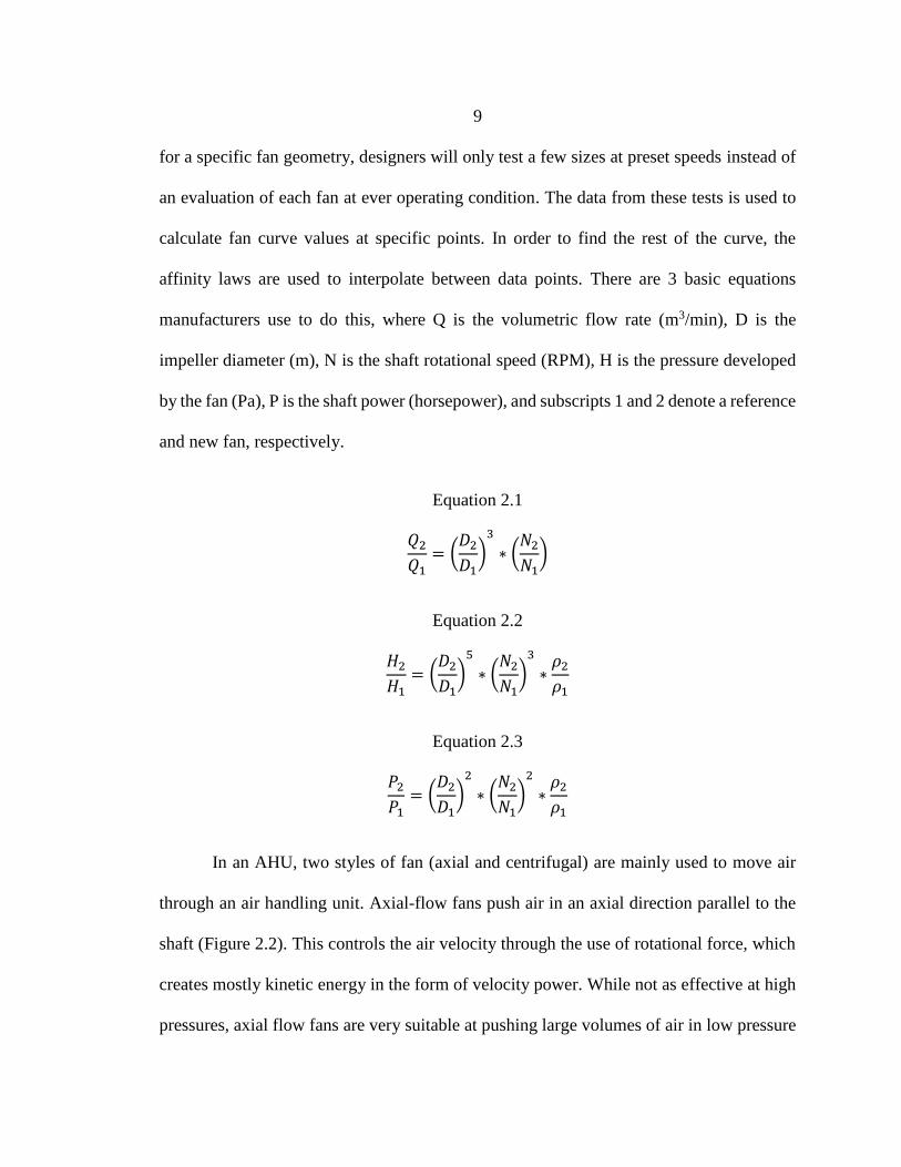
affinity laws are used to interpolate between data points. There are 3 basic equations
manufacturers use to do this, where Q is the volumetric flow rate (m3/min), D is the
impeller diameter (m), N is the shaft rotational speed (RPM), H is the pressure developed
by the fan (Pa), P is the shaft power (horsepower), and subscripts 1 and 2 denote a reference
and new fan, respectively.
Equation 2.1
𝑄2
𝑄1= (
𝐷2
𝐷1)
3
∗ (𝑁2
𝑁1)
Equation 2.2
𝐻2
𝐻1= (
𝐷2
𝐷1)
5
∗ (𝑁2
𝑁1)
3
∗𝜌2
𝜌1
Equation 2.3
𝑃2
𝑃1= (
𝐷2
𝐷1)
2
∗ (𝑁2
𝑁1)
2
∗𝜌2
𝜌1
In an AHU, two styles of fan (axial and centrifugal) are mainly used to move air
through an air handling unit. Axial-flow fans push air in an axial direction parallel to the
shaft (Figure 2.2). This controls the air velocity through the use of rotational force, which
creates mostly kinetic energy in the form of velocity power. While not as effective at high
pressures, axial flow fans are very suitable at pushing large volumes of air in low pressure

10
applications. These types of fans are used in applications such as industrial dryers, or air
conditioning units. Efficiencies of axial fan types are generally around 70-72% [23].
Figure 2.2: Axial flow fan wheel (left) and airflow direction (right)
Figure 2.3: Centrifugal fan impeller wheel (left) and airflow direction (right) [23]
Centrifugal fans are the most common type of fan utilized in an AHU (Figure 2.3).
Both centrifugal force and rotational velocity of the blades propel air in the radial direction
perpendicular to the shaft. This produces energy in the form of both static and dynamic
pressure. Centrifugal fans are best suited for high-pressure applications, such as for
drawing air through the total resistance in a HVAC system. Where axial fans have straight

11
blades extruding out from a central hub, centrifugal fans can choose from both forward and
backward curved impeller blade designs (Figure 2.4). Forward curved (FC) fans generally
operate at lower speeds and pressures, allowing lighter construction for fan components.
This results in a low-cost fan that can move large amounts of air at lower static pressures.
FC fans can become unstable and inefficient as a plenum (unhoused) fan, and require the
use of a fan housing (Figure 2.5) to help convert the higher levels of dynamic pressure
created by the fan into static pressure. The efficiency of FC fans can be in the range of 65-
70%, although their performance is highly dependent on the housing used to redirect the
flow [23]. Backward curved (BC) fans are more heavily constructed as they generally
rotate at higher speeds than forward curved fans do for the same static pressure rise. This
means that BC centrifugal fans have a larger upfront cost, but they are capable of being
used for applications with higher static pressure requirements and recovers the cost in the
long-term. Efficiencies are better than that of FC fans, being in the 75-80% range [23].
Because more of the energy of a BC fan is in the form of static pressure than a FC fan, it
loses less energy converting dynamic pressure to static pressure and is suitable for use
without a house.
Figure 2.4: Forward curved vs backward curved centrifugal fan blade designs [23]

12
Figure 2.5: Fan housing
Heat Exchangers
Heat exchangers, otherwise referred to as heating or cooling coils, are used to
transfer heat from one medium to another in many HVAC applications including space
heating, refrigeration, and air conditioning. There are many forms of heat exchangers,
however two of the main types will be briefly discussed below as they are commonly used
in HVAC systems.
A rotary-wheel heat-exchanger is a kind of heat-recovery system. Unlike most
types of heat exchangers, a rotary-wheel heat-exchanger does not use a second fluid or gas
to transfer heat from an external source to the airflow within an AHU. A large, permeable
wheel is rotated by a motor and allows air to pass through it. This material absorbs both
sensible (change in temperature) and latent (change in humidity)heat from the warmer air
side and transfers it to the colder air side where the airflow is traveling in the opposite
direction (Figure 2.6). This setup transfers the indoor conditions from the exhaust air to the
supply air just entering the building, reducing the amount of energy required for the AHU
to condition the fresh air.
13
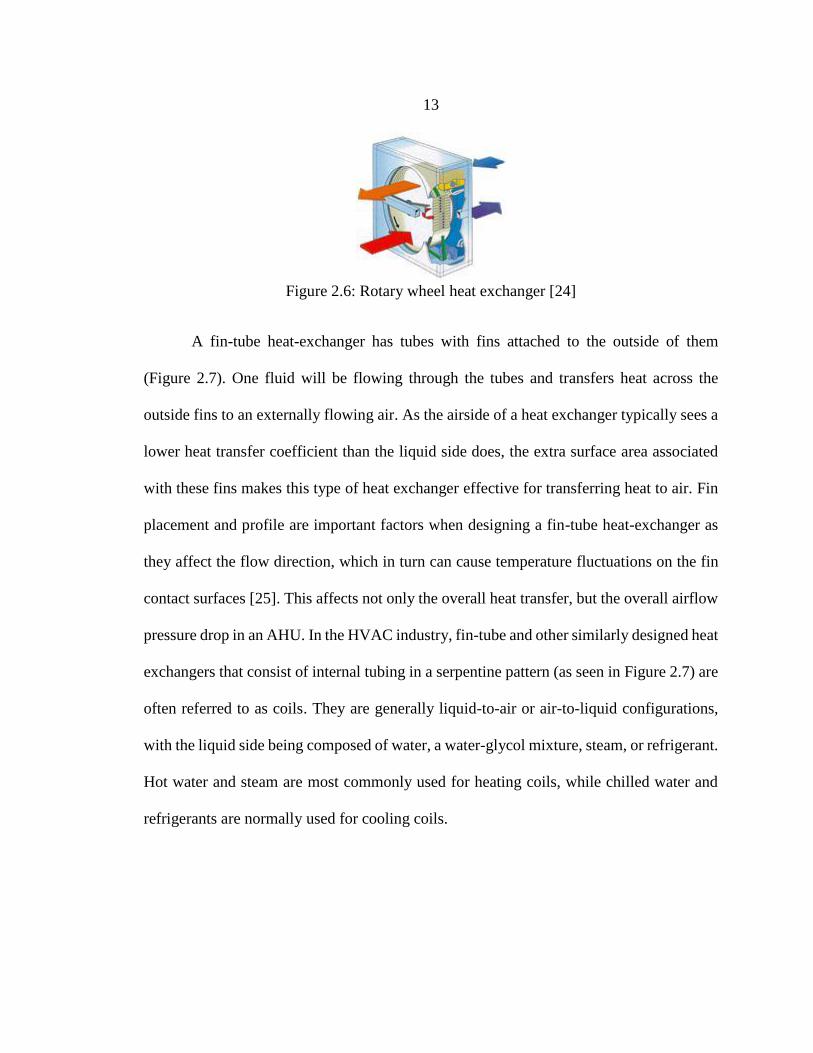
Figure 2.6: Rotary wheel heat exchanger [24]
A fin-tube heat-exchanger has tubes with fins attached to the outside of them
(Figure 2.7). One fluid will be flowing through the tubes and transfers heat across the
outside fins to an externally flowing air. As the airside of a heat exchanger typically sees a
lower heat transfer coefficient than the liquid side does, the extra surface area associated
with these fins makes this type of heat exchanger effective for transferring heat to air. Fin
placement and profile are important factors when designing a fin-tube heat-exchanger as
they affect the flow direction, which in turn can cause temperature fluctuations on the fin
contact surfaces [25]. This affects not only the overall heat transfer, but the overall airflow
pressure drop in an AHU. In the HVAC industry, fin-tube and other similarly designed heat
exchangers that consist of internal tubing in a serpentine pattern (as seen in Figure 2.7) are
often referred to as coils. They are generally liquid-to-air or air-to-liquid configurations,
with the liquid side being composed of water, a water-glycol mixture, steam, or refrigerant.
Hot water and steam are most commonly used for heating coils, while chilled water and
refrigerants are normally used for cooling coils.

14
Figure 2.7: A fin tube heat exchanger [25]
Like with fans, the performance of a heat exchanger is often measured by its
efficiency, where the efficiency can be defined by the ratio of the actual observed rate of
heat transfer to what the ideal calculated heat transfer is. The efficiency of a heat exchanger
can vary due to a number of causes. A decrease in thermal performance can occur due to
heat loss to the surrounding areas. Improper heat exchanger design can cause fouling of the
heat transfer fluid within the tubes which can create fluctuations in the heat transfer
coefficient across a heat exchanger, creating an uneven heat transfer profile. In this study,
of most importance is the uniformity of the flow across the heat exchanger as research has
shown that a non-uniform flow can lower the heat transfer rate across a heat exchanger [3].
While experimental measurements may locally indicate a complex flow occurring through
the heat exchanger, other methods of characterizing the flow are often required to show the
flow patterns that might indicate potential causes for flow non-uniformity upstream of a
heat exchanger in an AHU.

15
Computational Fluid Dynamics
CFD is a numerical method used to analyze fluid flow problems as a fluid travels
either through or around a specified domain. The two most commonly used formulations
for discretizing and solving the Navier-Stokes equations are the finite difference method
and the finite volume method [28]. The finite difference method (FDM) approximates
partial differential equations (PDE) by using a Taylor series expansion. This method is
easy to implement for simple problems, but requires a structured grid to do so. The finite
volume method (FVM) splits the geometry into multiple control volumes and uses an
integral approach to solve the physical conservation laws. The discretization for FVM is
applied directly to integral equations written for finite control volumes. While FDM is easy
to use with a structured grid, FVM is a more robust model, allowing the use of unstructured
grids while also exactly reproducing the principle of conservation across the entire
computational domain. Because of these benefits, FVM is used by the majority of
commercial and research CFD programs [28]. These methods can be used to solve for
either a steady-state flow (the velocity profile holds constant over time) or a transient one
(the velocity profile changes from time step to time step).
There exist many approaches to numerically analyze the turbulence of a flow in
CFD. The most common technique is by using the Reynolds-Averaged Navier Stokes
(RANS) equations which models the flow profile by using Reynolds decomposition to
decompose an instantaneous flow quantity into time-averaged and fluctuating flow
quantities. The RANS equations use approximations based on flow turbulence properties
to produce a time-averaged solution for the fluid flow. This process has the lowest

16
computational cost when compared to other methods, but the error from the approximations
of these quantities can create a more inaccurate result than with the different simulation
approaches. Other methods include the large eddy simulation (LES), detached eddy
simulation (DES), and direct numerical simulation (DNS). The LES method directly
calculates the mean flow as well as the unsteady large-scale and intermediate-scale motions
of the flow. The small-scale fluctuations in the flow are modeled, which introduces a
modeling error, albeit this error is generally smaller than in a RANS model. The
computational cost of LES is much higher than that of the RANS method The DES method
divides the flow domain into two layers; a core layer which is simulated using the LES
approach, and a near-wall layer which is modeled using the RANS approach. Because of
the use of a RANS model for this near-wall layer, the computational cost can be less than
when using a pure LES model to solve for turbulence. DNS is the most accurate method
available for solving the turbulence in fluids, directly solving the Navier-Stokes equations
for all aspects of a flow across a fine mesh. Of all the methods mentioned here, DNS has
the highest computational cost and is generally reserved for studies with simple flow
domains. [28]
Regardless of the methods used to solve for turbulence, CFD analysis has been
finding a wide application base in multiple areas of science and engineering, including the
aerodynamics of aircraft and vehicles, ship hydrodynamics, renewable energy, and even
biomedical engineering. The HVAC industry has increased their use of CFD as a design
tool in the past decade, looking at applications from server room temperature control to
characterizing the airflow across a cooling coil. Multiple examples where CFD is used to

17
analyze AHU components can be shown in the following section.
Although it is advised to initially validate CFD results from experimental data or
known solutions, once validation is completed, CFD can be used to model each iteration
of the optimization phase. The CFD model may not remain validated if the overall
geometry of the control volume is drastically changed. Depending on the computational
cost of the CFD simulations and the ability of the hardware used, multiple iterations with
a RANS formulation can be modeled and analyzed simultaneously on a single workstation.
The use of computational fluid dynamics in this study provides an easy method to
investigate a range of AHU configurations to and how it impacts flow uniformity and total
heat exchanged.
CFD in the HVAC Industry
Use of CFD analysis is by no means a new concept in the HVAC industry, and
there exists many studies which utilize CFD to analyze individual AHU components [29,
30]. Jain and Deshpande used CFD analysis to model the flow through an axial flow
radiator fan with right and left oriented blades, showing that the geometry of this type of
fan can create a high flow region along the outer diameter of the fan blades and a
low/reverse flow region directly behind the central hub of the fan [29]. Numerical results
showed a good correlation when compared with experimental data, with lower errors being
observed at higher flow rates. Chaudhary et al. numerically modeled a backwards curved
centrifugal fan to show that blades positioned at an increased angle to the flow produce a
larger pressure rise [30].
Although fans tend to create a rather turbulent flow regime where a transient

18
solution is more commonly desired, CFD analysis using a steady-state approximation is
possible. Atre and Thundil use a moving reference frame (MRF) with a steady-state
approximation to analyze the flow through a backwards curved centrifugal fan and
compare it with design data, showing a maximum deviation of 10% for all parameters
observed [31]. Sing et al. [32] also utilized a steady state MRF model for two different
prototype fans, showing a maximum error of 3% between the numerical and experimental
velocities at the fan casing outlet. The torque values required to run the fans also showed a
strong correlation at lower fan speeds; however, it is believed that frictional resistance of
the fan and mounting plate, as well as torsional vibration loads on the mounting shaft,
caused lower experimental values. CFD results diverged from experimental values at
higher fan speeds.
There are many examples of CFD analysis being used for different applications
with various types of heat exchangers, such as fluid flow uniformity, fouling, pressure drop,
and thermal analysis in both the design and optimization phase [33]. Ramachandran et al.
[34] studied the heat transfer and pressure drop characteristics over a ranger of Reynolds
numbers of plain fin and wavy fin heat exchangers in the external airside. CFD results were
validated using experimental data, and the solution showed that the number of tube rows
affected the heat transfer coefficient less as the number of rows increased. Also, tube
layouts in a staggered condition were observed to have better performance than in-lined
conditions for both types of heat exchangers. Knudsen et al. [12] analyzed the flow
structure and heat transfer in a vertical mantle heat exchanger. Experimental results found
using a PIV system showed a good correlation with numerical results, indicating that the

19
CFD model is able to simulate both the flow in the mantle and inner tank. Thermal analysis
also shows that a vertical mantle heat exchanger is also able to promote thermal
stratification, even with a negative heat flux at the tank walls.
Heat exchanger geometries can be highly complex, especially when creating a
numerical model of one. Incorporating these geometries into a CFD code can create a
higher computational cost. This longer computing time can be avoided by finding ways to
simplify the geometry. Kritikos et al. [35] modeled a heat exchanger using both the exact
geometry, as well as a porous medium. The porous medium behavior was described by
experimentally derived pressure drop as well as the heat transfer laws, where heat transfer
performance was characterized by the local Nusselt number. Numerical results from both
CFD models were in agreement with each other and with experimental results, indicating
that a porous medium can be used to model more complicated geometries. Hayes et al. [36]
similarly compared experimental data with results from a porous media model. Once the
accuracy of the numerical model was determined, it was modified to better simulate a
matrix heat exchanger. The modified CFD model results showed good agreement with
experimental results for Nusselt heat transfer correlations.
Flow non-uniformity within a system is a primary reason which results in poor
performance of heat exchangers. Non-uniformity in flow may be attributed to a number of
obstacles within the flow, such as improper design of flow inlets and outlets, baffles, and
even heat exchanger patterns. Many researchers have attempted to visualize or solve this
issue with the use of CFD [33, 37, 38]. Zhang et al. [37] simulated a plate fin heat exchanger
in order to optimize the header design at the inlet using the ratio of equivalent diameter.
20
CFD results showed a non-uniformity of the flow due to improper header design currently
used in industry. Two modified headers capable of two-stage distribution were then
analyzed and found to provide a more uniform fluid flow throughout the heat exchanger.
It was also found the flow was more uniform when the when the inlet and outlet diameters
are the same size. Wen and Li [38] have observed the effects that baffles with holes had on
fluid flow uniformity and effectiveness of plate heat exchangers. CFD analysis indicated
that baffles with smaller holes increased the uniformity from 0.05 to 0.68.
CFD analysis can be used to obtain the pressure drop across different filters. Feng,
et al. [39] assessed different turbulence models for predicting the airflow and pressure drop
through a pleated filter system (Figure 2.7), with the V2F (a particular set of turbulence
equations in the RANS formulation), DES, and LES models providing acceptable pressure
drop and velocity distribution values when compared with experimental data. The flow
uniformity was found for multiple types of filters using the relative root mean square error
(RRMSE) method, which compares the non-dimensionalized standard deviation of the
flow with the averaged measured velocity.
While there are many examples of how CFD has been used to model isolated AHU
components in an ideal setting, many of these studies do not take into account the real
world effects a full AHU system may incur on these components. Research involving these
real world effects taking into account the full AHU is limited to automotive HVAC
systems, such as in Jairazbhoy et al. [4], which used CFD to optimize the air flow through
a heat exchanger in an automotive HVAC system. The tight constraints imposed on these
automotive HVAC systems mean that the design is drastically different from a building
21
HVAC system. Because of this, a separate study is needed in order to verify CFD is a viable
alternative to the other physical methods of flow visualization, as well as to characterize
the airflow through a fully assembled AHU and to see the effects the flow structure may
have on heat exchanger performance.
Methods of Characterizing Flow
Flow Visualization
Flow-visualization techniques are useful for observing the large-scale flow-patterns
within a control volume. In an AHU, flow visualization can show areas of flow
recirculation within the geometry, flow separation along the AHU walls and the fan blades,
and potential obstructions in the flow path that could create a non-uniform flow. There
exists a number of ways to visualize flow; particle image velocimetry (PIV) uses a laser
light plane to illuminate small tracer particles that have been released into the fluid. Two
cameras then take images of this velocity field. PIV systems can provide excellent velocity
information at the inlet and outlet of the AHU; however, it requires high optical-access,
which proves difficult when trying to obtain data across the fan or other components. Laser
doppler anemometry (LDA) uses a laser beam split into two beams to measure the doppler
shift between the incident and scattered light caused by the particles within the flow. The
required optical access to the flow with LDA is significantly less than that of PIV systems,
which makes this method more suitable for observing the interior flow characteristics of
an AHU. While both PIV and LDA methods can be used to obtain an accurate
representation of the flow path, they are also rather expensive, requiring the purchase of
costly laser and camera equipment as well as a physical test model to be built. A less costly

22
method for flow visualization is smoke injection where smoke is added to the flow stream
and is used to show the flow path. This method can use multiple colors of smoke to show
any mixing that is occurring in the flow as well, but a physical test model is, again, required
and does not provide quantitative measurements.
As the method of particular interest in this study, CFD offers the ability to
numerically model an AHU. Although experimental data from a physical model is advised
to validate simulated results, it is not required for every iteration in the optimization process
and multiple geometric changes can be made to the base design to observe effects on the
flow profile simultaneously, such as the addition of baffles. The flow from CFD analysis
can be visualized using a number of different methods. Contour plots of scalar quantities
(Figure 2.8) can be used to show the velocity and pressure magnitudes which can indicate
the uniformity of the flow. Vector plots (Figure 2.9) can be used to show the direction of
the flow across a plane and magnitudes can be represented by both color and length of the
vector. Streamlines can show the flow path through a control volume, indicating potential
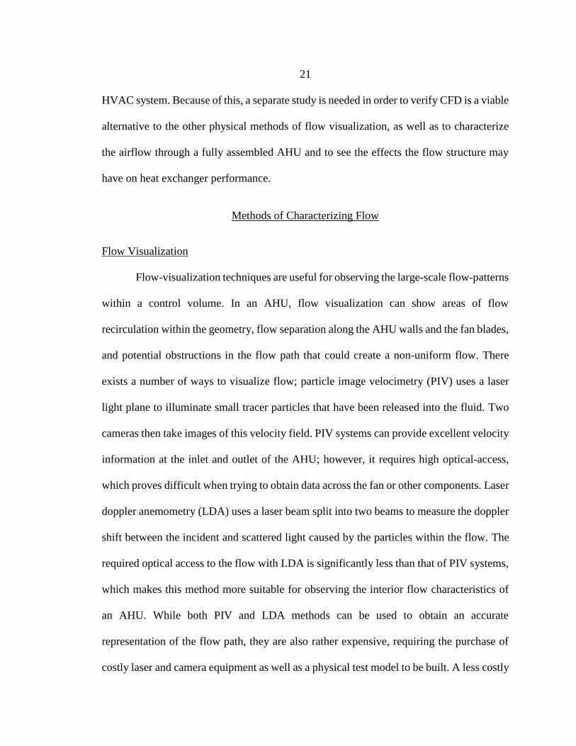
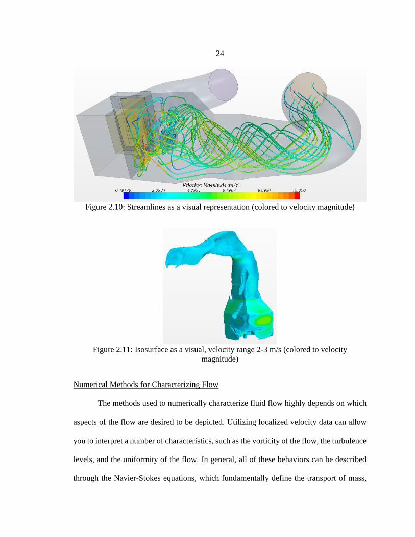
locations of turbulence, swirl, stagnating regions, etc. (Figure 2.10). An isosurface (Figure
2.11) is a surface that represents points of a specific value in a volume, and can be used to
show either a single value or a range of values.

23
Figure 2.8: Contours as a visual representation (velocity magnitude)
Figure 2.9: Vectors as a visual representation (velocity on a plane)
24
Figure 2.10: Streamlines as a visual representation (colored to velocity magnitude)
Figure 2.11: Isosurface as a visual, velocity range 2-3 m/s (colored to velocity
magnitude)
Numerical Methods for Characterizing Flow
The methods used to numerically characterize fluid flow highly depends on which
aspects of the flow are desired to be depicted. Utilizing localized velocity data can allow
you to interpret a number of characteristics, such as the vorticity of the flow, the turbulence
levels, and the uniformity of the flow. In general, all of these behaviors can be described
through the Navier-Stokes equations, which fundamentally define the transport of mass,

25
momentum, and energy of a fluid, or multiple fluids.
The velocity of the flow can tell us many things about the flow structure such as
the turbulence level, the uniformity of the flow, or identifying any vortices. As discussed
previously, the uniformity of the fluid flow has potential to impact the overall efficiency
of a system. The simplest definition of flow uniformity can be described as the deviation
of the velocity magnitude and direction from the average velocity across a control surface
or volume. In this study, this is achieved in two different ways. The first is by finding the
variance of the velocity values across a control surface or volume, where the velocity is
split into component values and the standard deviation values are found and non-
dimensionalized. This technique takes into account the standard deviation of each velocity
component value separately. The second method finds the unit vectors of both the average
velocity and the observed face velocity and finds the directional differences between the
two.
One of the major defining quantities when determining flow type is the Reynolds
number. The Reynolds number (Re) is a non-dimensional number used to determine if a
flow is laminar or turbulent, and is defined as the ratio between the inertial and viscous
forces acting on the fluid [26]. Lower Re values correlate with a laminar flow, but as the
velocity increases, the laminar boundary layer will become unstable and begin to transition
into a turbulent flow. For a pipe of diameter D, experimental observations show that a
laminar flow occurs when ReD < 2100 and turbulent flow occurs when ReD > 4000 [27]. A
flow with a ReD number between these values can have either laminar or turbulent flow
properties and is referred to as a transitional flow regime. Of course these values are for a

26
specific case with fully developed flow, and is subject to change depending on the
boundary conditions and fluid properties.
Turbulence is a classification of flow that can be described by highly-irregular
chaotic structures in the velocity field. The turbulence level of a flow can be characterized
through a number of different equations. Turbulence kinetic energy (TKE) is the mean
kinetic energy per unit mass in a flow as it deviates from the average, local velocity. TKE
is calculated as the root mean square (RMS) of the velocity fluctuations. This value can be
used to show the amount of kinetic energy in the flow across a region, or at localized points.
Another important quantity defining turbulence is the turbulence intensity (TI), which is
also referred to as the turbulence level, and is defined by the ratio of the root mean square
of the velocity fluctuations and the absolute value of mean velocity [28]. The turbulence
intensity provides a normalized value of how much the velocity fluctuates from the average
as a percentage. Without external forces, e.g. solar irradiation of the ground and the
corresponding temperature gradients, turbulent flows generally dissipate as it moves. This
dissipation, which is characterized by the turbulence dissipation rate, ε, is caused by the
kinetic energy braking into smaller turbulent structures before finally being converted into
thermal energy via viscous shear stress. The value of ε shows the reduction in the kinetic
energy of the flow due to the work performed in resisting fluid deformation by the
fluctuating strain rates.
A vortex can be visually recognized at points where there is rotational flow,
although the term itself lacks a firm definition. The analytic definition of vorticity is
defined as the curl of the velocity, and is equal to twice the rotation of the fluid at any point

27
in the flow-field [26]. Although this definition identifies regions of vorticity with a
corresponding magnitude, it does not specify which motions are caused by the rotational
energy in the flow (swirling motions) and those caused by the internal shear forces of the
fluid acting on itself (shearing motions). Three alternative definitions of vorticity can
provide additional information. Helicity is a scalar value generally seen as the amount of
swirl in the system and can be defined by the dot product of the velocity and vorticity, with
a higher value indicating a higher amount of swirl in the flow. The λ2-criterion searches
for a pressure minimum which can specify the low-velocity core at the center of a vortex.
This is done by splitting the Navier-Stokes equations into symmetric and anti-symmetric
parts. The Q-criterion defines a vortex as an area where the magnitude of vorticity is greater
than the rate-of-strain magnitude in the flow. Essentially, a vortex exists if the vorticity
tensor dominates the flow (Q > 0).

28
3 EXPERIMENTAL PROCEDURE
All experiments for this study took place in the psychrometric chamber inside the
HVAC lab at Montana State University. Three different experiments were conducted, the
first performed to obtain suitable pressure resistance coefficients to be used as the source
of the pressure drop from the cooling coil. The last two experiments were performed to
obtain experimental velocity values from the AHU without and with a baffle installed in
order to validate CFD results. The equipment used in these experiments to control the
airflow included an AAON V3-A AHU, and the custom unitary heat pump in the HVAC
lab. The AAON V3-A AHU, otherwise referred to as the AHU from this point, uses a
variable speed direct-drive, backward-curved plenum fan which produces a nominal flow
rate of 0.21-0.57 m3/s through the unit. This custom heat pump unit, otherwise referred to
the code tester from this point on, was built to match ASHRAE standards 37-2009 and 116-
2010, and produces a flow rate of up to approximately 0.81 m3/s. Equipment used to
measure experimental data included an Alnor 6050P-1 anemometer (±2% error) to measure
the air velocity, an Alnor AXD 560 micro manometer (±1% error) with Dwyer A-493
straight tip static pressure probes (±5% error) to obtain pressure data, and a Monarch Nova
Strobe DB Plus 115 stroboscope (±0.001% error) to measure the rotational speed of the
fan. The total error of the experimental velocity readings, shown in the results section of
this thesis, was computed as an accrual from the anemometer, the stroboscope, and the
variation seen in the fan speed. The error of the anemometer included not only the ±2%
from the device, but also a ±10 fpm due to the analog interface the flow rates were read
from. The minimum flow which could be read via this analog interface was 200 fpm,

29
meaning that lower velocity values hold a larger error than the higher flow rates do. During
the experiments, a shift in the fan speed of approximately ±2.5% was seen on a regular
basis as well.
Straight Duct
As will be discussed in more detail in the heating and cooling coil subsection of
Chapter 4, the heating and cooling coils were modeled as a porous region which prevented
the requirement for creating a more complex geometry and increasing the total
computational cost to run each simulation. These porous regions require the input of
resistance values to model the effects on the overall airflow within the AHU. Without
knowing these values, it becomes very difficult to predict the true flow characteristics. The
easiest way to obtain these values is to experimentally find the pressure drop across the
coil in question over a range of flow rates. The required coefficients can then be extracted
from this data and input into a numerical model as the coefficients for the Darcy-
Forchheimer law (Equation 4.1).
Test Setup
The pressure drop across the cooling coil installed in the inlet section of the AHU
needed to be found in order to properly model the air flow, as a change in the pressure drop
caused by the coil changes the flow rate through the coil, which can then change the
downstream flow conditions in the AHU. The first experiment achieved this by using a
straight duct (Figure 3.1), and the cooling coil from the AHU to find the pressure drop
across the coil over various flow rates. This experiment used the lab code tester unit as the
30
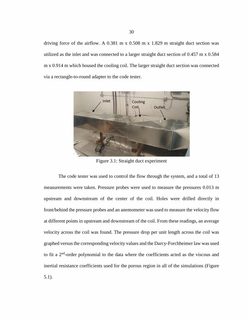
driving force of the airflow. A 0.381 m x 0.508 m x 1.829 m straight duct section was
utilized as the inlet and was connected to a larger straight duct section of 0.457 m x 0.584
m x 0.914 m which housed the cooling coil. The larger straight duct section was connected
via a rectangle-to-round adapter to the code tester.
Figure 3.1: Straight duct experiment
The code tester was used to control the flow through the system, and a total of 13
measurements were taken. Pressure probes were used to measure the pressures 0.013 m
upstream and downstream of the center of the coil. Holes were drilled directly in
front/behind the pressure probes and an anemometer was used to measure the velocity flow
at different points in upstream and downstream of the coil. From these readings, an average
velocity across the coil was found. The pressure drop per unit length across the coil was
graphed versus the corresponding velocity values and the Darcy-Forchheimer law was used
to fit a 2nd-order polynomial to the data where the coefficients acted as the viscous and
inertial resistance coefficients used for the porous region in all of the simulations (Figure
5.1).

31
Full AHU
Test Setup
For this thesis, experiments were run using a prototype AAON V3-A air handling
unit (Figure 3.2) in order to compare experimental data with CFD solutions. Equipment
used to measure the airflow velocity through the AHU included a stroboscope, and an
anemometer. Data taken included the velocity leaving the heating coil section of the AHU
(See Lines 1 and 2, Figure 4.3). Both the pressure drop and velocity data were taken at fan
rotational speeds of 1000 and 1800 rpm. The inlet and outlet of the AHU were each
attached to 0.5 m diameter openings via flexible duct which lead into the indoor room of
the psychrometric chamber. This allowed for the CFD model to initialize the flow coming
into the inlet duct as the cooling coil is located approximately 0.15 m from the opening.
Fan speed was controlled by a potentiometer dial located in the control box of the AHU.
The Stroboscope was used to confirm the rotational speed of the fan before any
experimental data was recorded. A marker was used on the top of the fan as an indicator to
see when the stroboscope was set to the right flash rate. Values of flash rate were directly
related to revolutions per minute (RPM) and no additional conversion was required to
obtain the true fan speed.
Velocity readings were taken across a plane in the outlet region, perpendicular to
the air flow direction. Holes just large enough to accommodate the anemometer were
drilled at the center point of the width and height of the duct at the locations of this plane.
Data was recorded in increments of 1 in along a straight line across the ducts at these points.
Across this plane, velocity values were taken in directions parallel and perpendicular to the

32
flow as allowed. Minimum, maximum, and average values were recorded at all points for
five separate samples in order to account for the transient nature of the airflow, as well as
with the inaccuracies that are inherent with an analog anemometer. Data collection was
performed this way with a fan speed of both 1000 rpm and 1800 rpm.
Figure 3.2: AAON V3-A Air Handling Unit
Baffles
Two wing baffles (Figure 3.3) were created and installed into the V3-A AHU
directly downstream of the fan before the reduced duct section (Figure 3.4). These baffles
were installed with the hopes that the rotational airflow seen in the previous experiment
would be funneled towards the center of the AHU before heading downstream. This would
ideally have the effect of improving flow uniformity. The previous experimental procedure
was repeated with velocity data being taken at each specified point across the same plane
as before. The change in experimental data caused by the baffles can be seen in the results
section

33
Figure 3.3: Wing baffle used in experiments
Figure 3.4: Wing baffle location
34
4 COMPUTATIONAL FLUID DYNAMICS METHODOLOGY
CFD has the capability to allow designers to visualize the airflow characteristics
through an AHU numerically in order to optimize the heating and cooling process without
building a physical test unit. The goal for this thesis was to utilize CFD to model the airflow
structure through an AHU and to quantify and visualize the effects that different baffles
and flow straighteners had on this flow structure. This section will summarize the methods
used to model an AHU with CFD and how the flow was numerically characterized.
Computational Fluid Dynamics Models
For this thesis a commercial CFD program, Star-CCM+®, was used to numerically
characterize the airflow pattern through an air handling unit. First, the cooling coil and its
physical parameters were calibrated using real world data, as detailed in Chapter 3. Next,
the CFD model for the AHU was created, which included all major items utilized in the
physical experiment. To reproduce the experimental results, a 3D parametric modeling
program was used to model all geometries, where the native file was then used to import
the geometry into Star-CCM+®. Simulated results were validated against experimental data
to set a reference for unobstructed flow through the unit. Different baffles and flow
straighteners were added to the CFD model then to analyze the effects they had on airflow.
The main interest was characterizing the downstream flow profile the fan created and
which methods were most efficient in creating a uniform flow profile.
35
Heating and Cooling Coils
Heating and cooling coils in general have a fairly complex geometry, which are
time consuming to recreate numerically and as a geometry sufficient for fluid modeling.
Even more so, when simulated using CFD, this geometry can greatly add to the
computational cost. In this study, replacing the actual cooling coil geometry with a
rectangular region proves to be a much more time-efficient practice and is much easier to
model utilizing Star-CCM+® due to there being no tube or fin geometry. While this
simplified geometry provides a less accurate solution by removing the mixing effects that
are normally caused by coil geometries, it greatly reduces the computational time required
to obtain a solution and still allows the coil to produce a pressure drop. This was acceptable
as the cooling coil was located upstream of the fan and was used primarily to model the
effect it had on the mass flow rate through the AHU. To achieve the pressure drop across
the cooling coil, porous viscous and inertial resistance values are assigned to this medium,
which are represented by the Darcy-Forchheimer Law (Equation 4.1), where β is the porous
viscous resistance, α is the porous inertial resistance, and 𝑈𝑛 is the superficial velocity
normal to the surface. What this represents is the pressure drop per length across the porous
medium. An experiment was created to calibrate the viscous and inertial losses, which can
be seen in the experimental procedure.
Equation 4.1: Darcy-Forchheimer Law
𝜕𝑝
𝜕𝑥= −𝛽 ∗ 𝑈𝑛 − 𝛼 ∗ |𝑈𝑛| ∗ 𝑈𝑛
A numerical model of the straight duct experiment was created to fine tune these

36
resistance values. The CFD model used to numerically model this experiment consisted of
only the inlet, outlet, and rectangle-to-round adapter geometries. A rectangular region was
created to model the coil geometry and was set as a porous region. The coefficients derived
from the experimental data shown in Figure 5.1 were used for the porous viscous resistance
(kg/m3-s) and porous inertial resistance (kg/m4) values in the airflow direction. Because it
was not desirable to characterize the flow disturbance caused by the coil itself, a value of
10,000 kg/m3-s and 10,000 kg/m4 were set for the resistance values in the lateral directions
(parallel to the x and z axis). This kept the flow unidirectional as it flows through the coil
in order to model drop in velocity values. The inlet boundary condition was set as a velocity
inlet, which controlled the flow rate in the model. The outlet boundary condition at the end
of the rectangle-to-round adapter was set as a pressure outlet. Inlet and outlet pressure
values were referenced to zero gauge at standard atmospheric conditions. The inlet velocity
was set to the same values as recorded in the experimental data. The pressure drop across
the coil was recorded and compared with the experimental data, shown as the pressure drop
per unit length (seen in Figure 5.1).
While heat transfer data was not experimentally recorded in this study, a heating
coil was included into some of the CFD models to assess how the baffles impacted the
amount of heat transferred to the flow. Like with the cooling coil region, the physical
characteristics of this heating coil were not based off of real world properties but instead
as a rectangular porous region. In addition to the assumption that this region produced the
same pressure drop per unit length as the cooling coil, the porosity was also set to 0.4,
which reduced the available open space within the region to 40%. This algorithmically

37
affected the density in the momentum equations when dealing with heat transfer. An input
of 15 kW was used as the heat source which drove the heat transfer through the region.
Full AHU
Air handling units can come in many different sizes and configurations, and can
include many different components. Only one air handling unit layout was used for this
thesis, which focused on characterizing the airflow in the area of interest, downstream of
the blower unit. The CFD models of the AHU included the same components used in the
experimental tests, which included the base assembly, blower unit, the cooling coil, and
the flexible duct attached to both the inlet and outlet. The inlet was modeled to obtain a
more developed flow as it enters the blower unit, and the cooling coil to produce an
accurate drop in velocity. The AHU was split into 4 different regions for the inlet, the
cooling coil, the fan, and the outlet (Figure 4.1). Like in the experiment, the blower unit
acted as the driving force of the airflow. To represent this, a cylindrical rotating region was
created and centered on the rotational axis of the fan. This resulted in setting the inlet
boundary condition as a stagnation inlet to allow the proper amount of air to be drawn
through the system towards the blower unit, and the outlet boundary condition as a pressure
outlet, with both boundaries being referenced at standard atmospheric conditions and gauge
pressure. Rotational speeds of 1000 and 1800 rpm were applied to the rotating region to
mimic the fan speeds used during the experimental procedures. While all other boundaries
besides the inlet and outlet were set as a wall boundary type, neighboring regions were
connected through stationary interfaces, allowing the air to flow between regions as
required. As explained previously, the cooling coil was modeled as a porous region to

38
simulate the pressure drop observed from real world data. Separate CFD models of the
AHU were created to include the wing baffle seen in the experimental procedure.
Figure 4.1: Full AHU model with regions
Simplified AHU
Computers using an Intel® Xeon ® CPU E5-1607 processor and 32 GB of installed
memory (RAM) were used to run the full AHU models with a fan rotation of 5o per time
step. While a solution time of approximately 3 to 4 seconds provided enough time to reach
a fully developed flow in the AHU, a minimum solution time of 7 seconds was required to
verify this. Using a total of 4 cores from the processor allowed a fully developed flow to
be verified in 2 weeks real time. To reduce the computational time, a simplified AHU
model was created to exclude unnecessary geometries in the CFD model (Figure 4.2). To
accomplish this, any geometry upstream of Plane 1 (Figure 4.3) was removed from the
AHU model. This eliminated the regions with the highest computational cost (the rotational
region and the cooling coil), and any other geometry that was not of interest to this study

39
(the inlet region). As the full AHU utilized the rotational motion of the fan to produce a
velocity and pressure field, the exclusion of this region required new initial conditions to
be found. To provide these initial conditions, velocity, TKE, and turbulence dissipation
rate data from the transient flow was recorded on Plame 1 from the full AHU model (Figure
4.3) over multiple time steps.
Up until this point, all of the CFD models created in this study utilized a transient
solution to solve for the flow due to the rotational motion created by the fan. In fluid
mechanics, transient flow refers to the condition where the fluid properties at each specific
point in a system changes from time step to time step. In CFD, the computational cost can
be dominated by necessarily reaching a fully developed flow from initial conditions. This
can be substantially reduced if a steady-state simulation is utilized under appropriate
conditions, which ultimately can allow the accrual of usable data at a much quicker rate.
With the fan region removed, the simplified CFD models could potentially utilize a steady-
state flow solution to further reduce the time required to obtain a fully developed flow from
simulated data. In order to justify the use of a steady-state solution, the variance of the
velocity components in each cell across Planes 1, 2, and 3 were found, with a variance of
0 m/s indicating the flow does not change at all. Additionally, a linear regression study was
conducted for the cells to see how the average velocity value changed over time. With this
method, a line slope of 0 m/s2 indicated a steady state flow could indeed be used. Each
simplified AHU model was then run with both a transient and a steady-state simulation and
compared to the solutions from the full AHU model. The time-averages across Plane 1
were used as the inlet initial conditions in the simplified AHU models. Once the flow

40
characteristics were observed from these models, a heating coil region was added to each
one to observe the effects that different flow structures had on the heat transfer in the AHU.
Figure 4.2: Simplified AHU with heating coil region
Figure 4.3: Location of Planes 1, 2, and 3 and Lines 1, and 2

41
Baffle Design
Once the simplified AHU models had been validated, different baffles were added
to the geometry downstream of the fan as wall boundaries. The purpose of this was to
observe the effect it had on the airflow characteristics in addition to the heating coil
performance. Baffles were created in a 3D CAD program and imported much like the
original AHU model was. Three different baffle designs were analyzed, which were added
to the outlet geometry and meshed using the same models, although smaller mesh sizes
were assigned to the baffle volumes as required to obtain a better mesh quality around the
perforated holes. The wing baffle (Figure 3.3) was designed to redirect air from the outer
walls of the AHU back to the center where a deficit in the airflow appeared to occur directly
downstream of the fan motor in the base AHU model. The other two designs included
perforated plates of two different geometries which spanned across the entire Plane 1 cross
section. The first of these perforated plates utilized 0.025 m diameter holes, uniformly
spaced across the entire plate, which was intended to straighten the flow and allow the
same amount of airflow through each hole (Figure 4.4). The second perforated plate
utilized three different diameter sized holes, with 0.013 m diameter holes along the border
of the plate, followed by 0.019 m holes closer to the center of the duct and 0.025 m holes
in the direct center of the plate (Figure 4.5). The intention of this design was to allow more
airflow through the plate where a velocity deficit occurs (the center), thus creating a more
constant volumetric flow rate across the plate and an even more uniform flow in the
downstream flow regime. While not normally used as a baffle design in an AHU, the
overall objective with using either perforated plate was to straighten the flow and help

42
dissipate the rotational pattern created by the blower unit in an effort to induce a drastic
change in the flow uniformity and turbulence levels. The inlet conditions used for the
simplified wing baffle model came from the full wing baffle AHU model. As a full AHU
model with either perforated plate was not previously created, both the simplified
perforated plate models used inlet conditions across Plane 1 from the base AHU. This was
deemed appropriate for rapidly creating a model with either perforated plate, as they were
meant to straighten out the flow.
Figure 4.4: First perforated plate: uniform hole pattern using 0.025 m diameter holes
Figure 4.5: Second perforated plate: a layer of 0.013 m holes around the edge, 0.019 m
holes in between this layer and the center, and 0.025 m holes in the center.
Meshing
Meshing a geometry splits it into a finite amount of control volumes, where the
conditions of the flow are solved for at the center of each of these control volume
43
individually. The CFD simulations used a surface remesher model to create a surface mesh
of the geometry of each of the 4 regions. Two main types of volume meshes are used in
CFD, tetrahedral and polyhedral. A tetrahedral mesh could easily have been used to provide
the volume mesh, however polyhedral meshes were used due to it providing the same level
of accuracy while using approximately five times fewer cells when compared to an
equivalent tetrahedral mesh [40]. A prism layer mesher was used around the fan and outlet
regions to increase the accuracy of the solution around both the smaller dimensions of the
fan blades and the interaction of the fluid flow with the duct walls. Star-CCM+® controls
the size of the surface and volume meshes in each continuum by specifying a base size.
Mesh cell sizes can then be fine-tuned by setting the target and minimum mesh sizes as
required, and can further be refined by assigning a specific mesh size to individual
boundary surfaces as well. The mesh size across a specific volume or surface within a
region can be controlled separately with the use of a surface or volumetric control, which
uses existing surfaces or separately created volumetric shapes to bound the chosen
area/volume and allows for a more desirable mesh to override the base mesh conditions.
Before the regions were created, a surface wrapper model was used to obtain an initial
surface mesh for the rotating region. This was required to obtain a sufficient, closed
geometry due to the complexity of the fan. Once an acceptable surface mesh was obtained,
the regions were created for the inlet, cooling coil, fan, and outlet and a volume mesh was
generated for each. A base size of 0.04 m was used, with a minimum size of 0.01 m and a
target size the same as the base size. A courser base mesh was chosen due to the less
complex geometry of the majority of the AHU. The rotational region specified a surface
44
size of 0.0005 m to account for the smaller geometry of the fan, and a volumetric control
was created directly around the fan geometry, using a mesh size of 0.015m. The fan region
used a smaller sized mesh as the rotating region required more detail to accurately simulate
airflow reaction with the fan blades. The outlet region utilized a total of 3 more volumetric
controls, the first being used to refine the mesh directly around the fan (and baffles). The
mesh used in this volumetric control was assigned to 0.0175 m in order to better
characterize the vortex shedding caused by the fan blades and the shear rate caused by the
fluids interaction to the duct walls. The next volumetric control continued downstream
from the first, through the reduced duct section, and used a mesh size of 0.02 m. The third
used a cylindrical volume, focusing on the center of the duct. A 0.01 m mesh size was
chosen for this control, as it was desirable to obtain a more detailed picture of any vorticity
occurring in this section. Both the inlet and the evaporator regions, as well as the remainder
of the outlet region, used the base mesh conditions as a detailed observation of the flow in
these sections was not a part of this study. The final mesh count for the full AHU models
varied between approximately 579,000 cells to 720,000 cells.
CFD Flow Characterization
As described before, many ways exist to numerically portray the flow through an
AHU. For this thesis, the Reynolds Average Navier-Stokes (RANS) equation (Equation
4.2) was used to model the airflow through the air handling unit. This method is perhaps
the most widely used CFD solver, and uses Reynolds decomposition to separate the
fluctuating and time averaged quantities from the Navier-Stokes equations. Although the
LES model may provide a more exact solution by discretely solving for the large and

45
intermediate-scale motions of the flow, the accuracy versus computational cost of the
RANS equation was desirable. The simulated airflow showed very small changes in
temperature, density, and pressure relative to the velocity, which allowed an
incompressible flow assumption to be used. Due to the rotational flow caused by the blower
unit, a fully turbulent assumption can be considered accurate for this case as the airflow
moves downstream of the fan. Because of this assumption, a k-ε turbulence model was
paired with the RANS equations to solve for the turbulence flow structure.
Equation 4.2: Reynolds average navier-stokes equations
𝜌𝜕𝑈𝑖̅̅ ̅
𝜕𝑡+ 𝜌
𝜕
𝜕𝑥𝑗(𝑈�̅�𝑈�̅�) = −
𝜕�̅�
𝜕𝑥𝑖+ 𝜇𝛻2𝑈�̅� −
𝜕𝜏𝑖𝑗
𝜕𝑥𝑗,
𝜕𝑈𝑖̅̅ ̅
𝜕𝑥𝑖= 0
The k-ε turbulence model was chosen as it is the most widely used turbulence model
which requires initial and boundary conditions, and turbulence parameters to be run.
Methods for numerically characterizing the turbulence of the flow included the turbulent
kinetic energy (Equation 4.3) and the turbulence intensity (Equation 4.4). As stated
previously, the turbulent kinetic energy (TKE), k, can be described as the mean kinetic
energy per unit mass associated with eddies in turbulent flow, and can be characterized by
the mean of the turbulence normal stresses [41]. TKE can be a result of fluid shear, friction
acting on the fluid from an object, or external forces. If the turbulent kinetic energy is
known, then the turbulence intensity (TI), or the turbulence level of the flow, can be found.
Turbulence intensity can be described as the ratio of the root-mean-square of the turbulent
velocity fluctuations, 𝑈𝑖′, to the mean velocity of the flow, which is computed from the
three mean velocity components [42].

46
Equation 4.3: Turbulent kinetic energy
𝑘 =1
2[𝑈𝑥
′𝑈𝑥′̅̅ ̅̅ ̅̅ ̅̅ ̅ + 𝑈𝑦
′𝑈𝑦′̅̅ ̅̅ ̅̅ ̅̅ ̅ + 𝑈𝑧
′𝑈𝑧′̅̅ ̅̅ ̅̅ ̅̅ ]
Equation 4.4: Turbulence intensity
𝑇𝐼 =(2𝑘 3⁄ )1 2⁄
(𝑈𝑥̅̅̅̅ 2
+ 𝑈𝑦̅̅̅̅ 2
+ 𝑈𝑧̅̅ ̅2
)
In addition to the RANS and k-ε turbulence models, a segregated flow solver was
chosen as the flow regime solver for this model. Compared to a coupled flow solver, the
segregated solver requires less computational time and memory to run as it solves the
governing equations (continuity, momentum, and energy) sequentially. It is also ideally
suited for incompressible flow, whereas the coupled flow model would be the better choice
for compressible, supersonic flow models. Because the segregated flow and turbulence
models were chosen, an implicit unsteady transient model was selected for the AHU model.
Two different methods were used to characterize the uniformity of the airflow, the
relative root mean square error and flow uniformity. The relative root mean square error
(RRMSE) method (Equation 4.5), used in Feng et al. [39], is used in this thesis as the first
of these two methods with 𝑈𝑖 being the vector-component of the observed velocity value,
�̅�𝑖 being the average velocity value, and N being the number of total points the velocity
data is taken from. The main difference seen in this study is that the flow being observed
is multi-directional, whereas in Feng et al. it was unidirectional as it traveled through a
pleated filter. Flow uniformity is also calculated from the dot product of the unit vector of
the observed velocity with the unit vector of the average velocity (Equation 4.6). This
47
method is able to assign a length of 1 to both vectors, still pointed in the direction of the
original vector, and uses the dot product to compare the direction of the observed velocity
values with average values. Scalar resultants from the dot product can then be used to show
the flow uniformity as a percentage of how much the actual flow deviates from a fully
uniform flow. While both methods are used to measure the differences between the
detected and average values, the RRMSE methods seeks to measure the variance in the
values of each velocity component, where the uniformity method in Equation 4.5 finds the
difference in direction between the velocity vectors and average velocity vectors.
Equation 4.5: Relative root mean square error
𝑅𝑅𝑀𝑆𝐸 = √∑ (𝑈𝑖 − 𝑈𝑖)2
𝑁1
𝑁 − 1𝑈𝑖⁄
Equation 4.6: Flow uniformity
𝑈𝑛𝑖𝑓𝑜𝑟𝑚𝑖𝑡𝑦 = 𝑈𝑖
|𝑈𝑖|∙
𝑈�̅�
|𝑈�̅�|
Many of the methods used to characterize the vorticity of the flow are explained in
depth in Holmen et al. [26], and are based off of the velocity gradient tensor, Dij (Equation
4.7), which is a second order tensor consisting of both a symmetric and skew-symmetric
part. The symmetric part, Sij, is known as the rate-of-strain tensor (Equation 4.8) and the
skew-symmetric part, Ωij, is the vorticity tensor (Equation 4.9).
Equation 4.7: Velocity gradient tensor
𝐷ij = 𝑆ij + 𝛺ij

48
Equation 4.8: Symmetric part of the velocity gradient tensor
𝑆ij =1
2(𝜕𝑈𝑖
𝜕𝑥𝑗+
𝜕𝑈𝑗
𝜕𝑥𝑖)
Equation 4.9: Skew-symmetric part of the velocity gradient tensor
Ωij =1
2(𝜕𝑈𝑖
𝜕𝑥𝑗−
𝜕𝑈𝑗
𝜕𝑥𝑖)
Finding the characteristic equation for the velocity gradient tensor (Equation 4.10),
∇U, provides the three invariants of the velocity gradient tensor, with λ being the
eigenvalues of ∇U. These invariants, P, Q, and R, can be expressed as shown in Equations
4.11, 4.12, and 4.13 below. The Q-criterion uses the second invariant of the velocity
gradient tensor (Equation 4.12) to define a vortex as a spatial region where the Euclidean
norm of the vorticity tensor, Ωij, dominates that of the rate of strain tensor, Sij [43]. Simply
stated, if the vorticity magnitude is greater than the magnitude of the rate of strain tensor,
then Q > 0 and a vortex can be said to exist within the flow.
Equation 4.10: Velocity Gradient Tensor, ∇u
𝛻𝑈 = 𝜆3 + 𝑃𝜆2 + 𝑄𝜆 + 𝑅 = 0
Equation 4.11: First Invariant of the Velocity Gradient Tensor, P
𝑃 = −𝑡𝑟(𝐷)
Equation 4.12: Second Invariant of the Velocity Gradient Tensor, Q
𝑄 =1
2‖𝛺ij‖
2− ‖𝑆ij‖
2

49
Equation 4.13: Third Invariant of the Velocity Gradient Tensor, R
𝑅 = −𝑑𝑒𝑡 (𝐷)
The λ2-criterion (Equation 4.14) uses part of the gradient of the Navier-Stokes
equations, eliminating the unsteady irrotational straining and viscous effects, or S2 + Ω2.
This equation is used to determine if there is a local pressure deficit which indicates a
vortex is present in the flow or not. In this case, a vortex is defined as “a connected region
with a negative eigenvalue of S2 + Ω2”, which indicates λ2 is a real, negative value when a
vortex is present [26].
Equation 4.14: λ2-criterion
−1
𝜌𝑝𝑖𝑗 = Ω𝑖𝑗Ω𝑘𝑗 + 𝑆𝑖𝑘𝑆𝑘𝑗
The vorticity, ω, is found via the curl of the velocity (Equation 4.15). Like with
quantities such as velocity, pressure, and temperature, a vortex can be visualized using
isosurfaces, however the threshold used in 3D flows can have a tremendous effect on the
visualized vortex structure since vorticity can often span over many orders-of-magnitude
in a flow field.
Equation 4.15: Vorticity
𝜔 = 𝛻 × 𝑈
Helicity is a quadratic invariant of the Euler equations for ideal-fluid flow, which
represents the degree of linkage of the vortex lines, or the line which is everywhere tangent
to the vorticity vector [44]. While the vorticity is a vector field, the helicity is a scalar value
that expresses the connection between the spinning motion and the linear motion of a flow.
50
This scalar value can be found through the dot product between the velocity and the
vorticity (Equation 4.16).
Equation 4.16: Helicity
𝐻 = 𝑈 ∙ 𝜔
The methods previously described in this section will be used in this study to
characterize the airflow through an AHU. Values for the uniformity (Equation 4.5,
Equation 4.6), turbulence (Equation 4.3, Equation 4.4), and vorticity (Equation 4.12,
Equation 4.14, Equation 4.15, Equation 4.16) will be analyzed. From here, different baffles
will be included in the AHU geometry, and the effects that these baffle geometries have on
the downstream flow characteristics of the AHU will be compared with base values to see
if the flow uniformity has improved or not.

51
5 RESULTS
The results from the experiments and CFD models previously mentioned in this
thesis will be used to further investigate the airflow characteristics through each model,
and the effects that different baffles may have on the performance level of this particular
AHU. Experimental results from the straight duct experiment were first used to find the
required resistance coefficients used to simulate the pressure drop through the cooling coil.
Velocity values from the base and wing baffle AHU models were then compared with
experimental data, with a good correlation being seen overall. Data was then compared
between the full and simplified AHU models, where a simplified, steady-state AHU model
provided to be an excellent surrogate to rapidly simulate models with perforated plate
baffles. The results from these simplified AHU models were then numerically
characterized to present the effects each baffle had on the downstream flow structure
relative to baseline results. Finally, the models were then used to assess the impact each
baffle had on the heat transfer through a heating coil region compared to values seen from
the base AHU model.
Straight Duct
The pressure measurements taken from the straight duct experiment were used to
understand the specific loss the cooling coil would have on the system. Because the CFD
model represented the coil as a porous continuum, and not as an explicit geometry, the
experimental data are used to determine the porous inertial and viscous resistance
coefficients according to the Darcy-Forchheimer law (Equation 4.1). The parameters

52
simulate the pressure drop, as a function of velocity, and alter the body force in the
momentum equations. Due to the polynomial order of the Darcy-Forchheimer law a
quadratic equation was best-fit to the experimental data and gave a porous inertial
resistance of 44.658 kg/m4 and viscous resistance of 109.36 kg/m3-s. CFD simulations were
performed with the inertial and viscous losses applied to the porous region over a range of
flow rates between 0.17-0.80 m3/s. Figure 6.1 shows the experimental and simulated results
from the straight duct experiment. The porous region approximation provides a very good
fit at lower velocities, but begins to increase in error after flows of approximately 2.5 m/s.
This deviation from the quadratic fit may be due to transition in the system from laminar
to turbulent flow, and the growing error is a possible contributor to any potential
inaccuracies seen in the AHU models in the next sections.
Figure 5.1: Simulated vs experimental pressure drop data for the cooling coil

53
Full AHU
Base AHU
Experimental data shows a highly non-uniform flow in the downstream section of
the AHU. The velocity magnitude and direction were broken into Cartesian components,
with a z-part traveling in the downstream direction and x- and y-parts traveling laterally
across Lines 1 and 2 from Figure 4.3. It is important to note that due to the orientation of
the AHU in the HVAC lab the measurement equipment was not able to collect data along
the entirety of Line 1, missing 0.17 m. Velocity component data for the 1000 RPM fan
speed shows a distinctive deficit in the airflow structure, with observed downstream
component velocity values showing a low flow of 0 m/s in the center of the duct and a high
of 1.5 m/s near the walls of the AHU. The lateral components at this fan speed indicate a
highly rotational flow with, again, very low velocity values located in the center of the duct
and a high of 2 m/s near the AHU walls. This deficit becomes more apparent at the 1800
RPM fan speed, with velocities near the wall doubling in value while the downstream
component of velocity increases to 1 m/s in the center of the duct. These experimental
values show a flow structure that is highly dominated by rotational flow, creating a low
flow area in the center of the duct and allowing the majority of the flow to travel along the
walls of the AHU.
Comparing the experimental measurements from the AHU to simulated results
shows the value of CFD simulations as a tool for design and analysis. The comparison of
component-velocity data taken along Lines 1 and 2 (Figure 4.3) for the baseline AHU can
be seen in Figures 6.2-6.5, with (a) representing the downstream component and (b) the

54
lateral components. There is good agreement between experimental and simulated values
for the lateral components of velocity (Figure 6.2(b)). The z-component of velocity in
Figure 6.2(a) shows a profile similar to the one seen from experimental data; however, an
offset is evident between experimental and simulated values of approximately 0.5-1 m/s
(1.64 – 3.28 ft/s) near the center of the duct. A similar offset of velocity values is also seen
at the walls for both the lateral and downstream velocity components in each of the data
sets. The simulations did not fully capture the plug-like flow that existed directly over the
blower, although the discrepancies seen in this comparison are possibly due to additional
error associated with the low velocity range of the anemometer used in the experiments.
Different turbulence models should be evaluated as well, as it is possible the flow-field is
mixing too much and diffusing the flow structure evident in the experimental
measurements.
Figure 5.2: Base AHU 1000 RPM experimental vs simulated velocity data from Line 1
(a) z-component (b) x-component velocity

55
Figure 5.3: Base AHU 1000 RPM experimental vs simulated velocity data from Line 2
(a) z-component (b) y-component velocity
Figure 5.4: Base AHU 1800 RPM experimental vs simulated velocity data from Line 1
(a) z-component velocity (b) x-component velocity

56
Figure 5.5: Base AHU 1800 RPM experimental vs simulated velocity data from Line 2
(a) z-component velocity (b) y-component velocity
AHU with Wing Baffle
The goal of using the wing baffle design seen in Figure 3.3 was to redirect some of
the airflow traveling along the walls of the AHU to the center of the duct where a velocity
deficit was obvious. Experimental data from the AHU with this baffle installed showed
that while downstream velocity values along the AHU walls remained mostly unchanged,
velocity values in the center of the flow were increased. Data seen for the downstream
velocity component across both lines show an increase in the minimum values of
approximately 0.8 m/s; however, the flow structure across Line 1 appears to have
potentially shifted in a manner that moves the velocity deficit away from the center of the
duct. Observation of the lateral velocity components show a decrease of 0.5 m/s in the
maximum velocity magnitudes as well, indicating that the baffle has helped to reduce the
rotational aspect of the flow in favor of a more downstream trajectory.
This reduction in the rotation of the flow is also seen in the simulated results,

57
showing in Figures 5.6(b) - 5.9(b) that the CFD model again is able to match the rotational
portion of the flow observed from the experimental data. Some overestimation in the CFD
solution still occurs along the walls of the AHU, which may be the result of the anemometer
wand affecting the near wall flow structure in the experiments. Observation of the velocity
z-component data across Line 1 (Figure 5.6(a), Figure 5.8(a)) shows that while the
minimum velocity values was increased by approximately 0.25 m/s when compared to
baseline values, the CFD results did not follow the apparent shift seen in the experimental
data, and the simulated velocity deficit still remains at the center of the duct. More so,
simulated values on Line 1 show a larger overestimation in the velocity values of
approximately 1 m/s at one of the AHU walls. While the velocity values appeared to have
reached steady state conditions (discussed in the next section), there could also be a flow-
structure evolution operating on a different time scale. Additionally, the choice of
turbulence model may have impacted the results across Line 1. Z-component velocity
values across Line 2 (Figure 5.7(a), Figure 5.9(a)) show a closer agreement between
experimental and simulated data, although values adjacent to the walls show a large
overestimation by the simulations and again may be impacted by the choice of turbulence
models, or an unknown flow structure development.

58
Figure 5.6: AHU with wing baffle, 1000 RPM experimental vs simulated velocity data
from Line 1 (a) z-component (b) x-component velocity
Figure 5.7: AHU with wing baffle, 1000 RPM experimental vs simulated velocity data
from Line 2 (a) z-component (b) y-component velocity

59
Figure 5.8: AHU with wing baffle, 1800 RPM experimental vs simulated velocity data
from Line 1 (a) z-component (b) x-component velocity
Figure 5.9: AHU with wing baffle, 1800 RPM experimental vs simulated velocity data
from Line 2 (a) z-component (b) y-component velocity
Overall, it appears that the addition of the wing baffle reduces the high velocity
deviation seen between the center and along the walls of the AHU with the central part of
the flow structure showing an increase in velocity z-component values of 0.8-1 m/s for

60
experimental data and 0.25 m/s for simulated results. A decrease in the amount of rotation
in the flow is also seen, with lateral velocity components showing a reduction of 0.5 m/s
in the velocity magnitudes. For future studies, collecting measurements across all of Plane
3 with finer spacing, instead of the two lines used here, would better identify the source
and amount of discrepancy.
Full Versus Simplified AHU
It was highly desirable to create a simplified AHU model in order to greatly reduce
the required computational time. Demonstrating that a near-steady flow exists at every
location on Planes 1, 2, and 3 was crucial for further simplifying the simulation. To do this,
component-velocity values were obtained for each cell across all three planes. A linear
regression equation and variance values of the velocity at each cell were calculated using
data from these planes. Figure 5.10 illustrates an example of the velocity values and the
linear regression lines typically seen from the base AHU simulated data. Velocity values
taken from the cells across Planes 1, 2, and 3 show a transient pattern that oscillates about
an average velocity value. Although the velocity acted in a transient nature, the variance
values indicated that the maximum variance values seen were negligible (on the order of
1e10-5 m/s), and the linear regression study showed the rate of change in the average
velocity values at each cell were insignificant. While Figure 5.10 shows fully developed
flow data over the course of 1.4 s, baseline AHU data was taken over approximately 14
seconds of simulation time (29,000 time-steps) which again confirmed these findings.
Although the downstream flow in the AHU appeared to be relatively turbulent and
rotational, this discovery verified that a steady-state flow assumption could be used. This

61
permitted the use of a much simplified geometry, consisting of only the portion of the full
AHU downstream of the blower, and a steady-state velocity profile in order to reduce
computational time.
Figure 5.10: Velocity and linear regression values on Plane 2 for the full AHU model,
1000 RPM, showing the a) x-component b) y-component c) z-component of velocity.
Base AHU
Once it was determined that the velocity data from Planes 1, 2, and 3 could be
considered acting at steady state, a simplified base AHU model was created. The inlet to
this new model uses the component-velocity and turbulence values from the full AHU at
Plane 1. The models were run as both transient and steady-state flows in order to compare
the accuracy of the results with data from the full AHU models. While the previous analysis
demonstrated nearly steady flows at all three planes, it needed to be ensured that moving
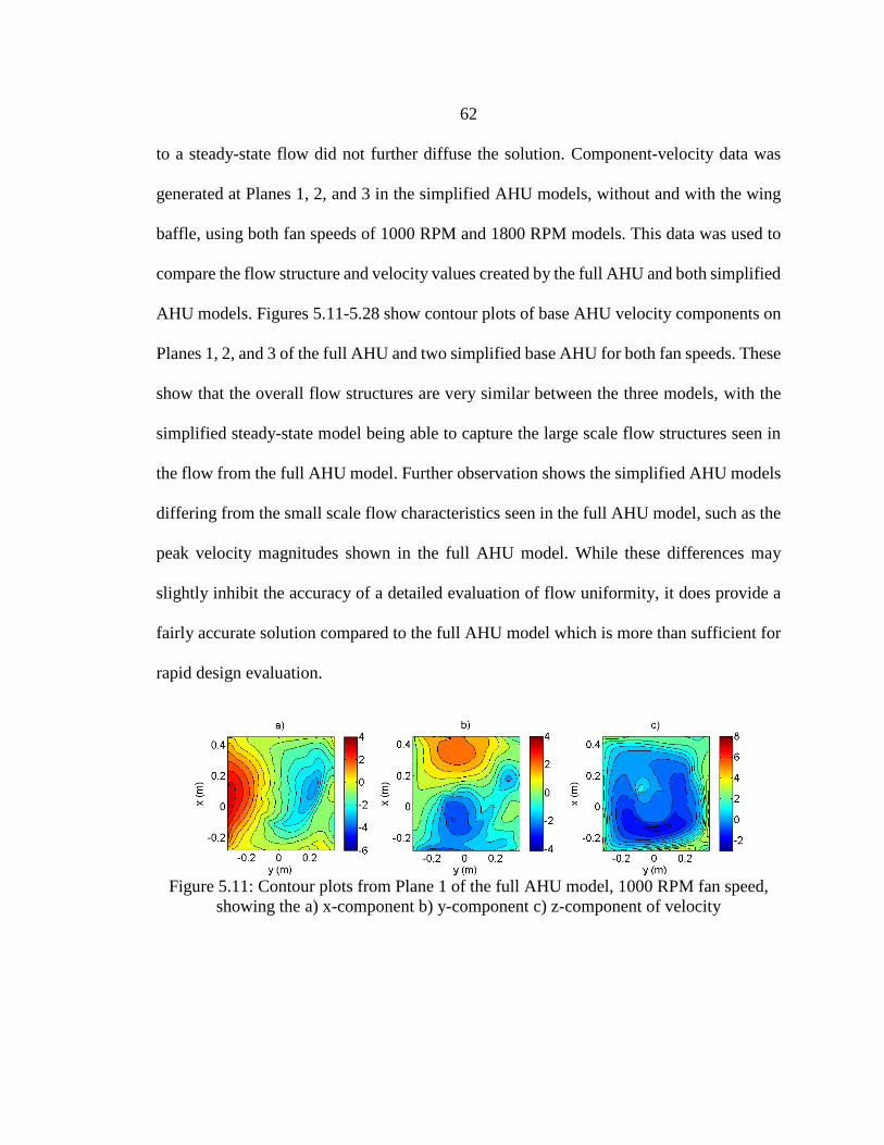
62
to a steady-state flow did not further diffuse the solution. Component-velocity data was
generated at Planes 1, 2, and 3 in the simplified AHU models, without and with the wing
baffle, using both fan speeds of 1000 RPM and 1800 RPM models. This data was used to
compare the flow structure and velocity values created by the full AHU and both simplified
AHU models. Figures 5.11-5.28 show contour plots of base AHU velocity components on
Planes 1, 2, and 3 of the full AHU and two simplified base AHU for both fan speeds. These
show that the overall flow structures are very similar between the three models, with the
simplified steady-state model being able to capture the large scale flow structures seen in
the flow from the full AHU model. Further observation shows the simplified AHU models
differing from the small scale flow characteristics seen in the full AHU model, such as the
peak velocity magnitudes shown in the full AHU model. While these differences may
slightly inhibit the accuracy of a detailed evaluation of flow uniformity, it does provide a
fairly accurate solution compared to the full AHU model which is more than sufficient for
rapid design evaluation.
Figure 5.11: Contour plots from Plane 1 of the full AHU model, 1000 RPM fan speed,
showing the a) x-component b) y-component c) z-component of velocity

63
Figure 5.12: Contour plots from Plane 1 of the transient simplified AHU model, 1000
RPM fan speed, showing the a) x-component b) y-component c) z-component of velocity
Figure 5.13: Contour plots from Plane 1 of the steady-state simplified AHU model, 1000
RPM fan speed, showing the a) x-component b) y-component c) z-component of velocity
Figure 5.14: Contour plots from Plane 2 of the full AHU model, 1000 RPM fan speed,
showing the a) x-component b) y-component c) z-component of velocity
Figure 5.15: Contour plots from Plane 2 of the transient simplified AHU model, 1000
RPM fan speed, showing the a) x-component b) y-component c) z-component of velocity

64
Figure 5.16: Contour plots from Plane 2 of the steady-state simplified AHU model, 1000
RPM fan speed, showing the a) x-component b) y-component c) z-component of velocity
Figure 5.17: Contour plots from Plane 3 of the full AHU model, 1000 RPM fan speed,
showing the a) x-component b) y-component c) z-component of velocity
Figure 5.18: Contour plots from Plane 3 of the transient simplified AHU model, 1000
RPM fan speed, showing the a) x-component b) y-component c) z-component of velocity
Figure 5.19: Contour plots from Plane 3 of the steady-state simplified AHU model, 1000
RPM fan speed, showing the a) x-component b) y-component c) z-component of velocity
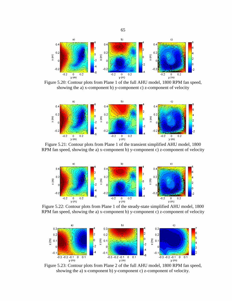
65
Figure 5.20: Contour plots from Plane 1 of the full AHU model, 1800 RPM fan speed,
showing the a) x-component b) y-component c) z-component of velocity
Figure 5.21: Contour plots from Plane 1 of the transient simplified AHU model, 1800
RPM fan speed, showing the a) x-component b) y-component c) z-component of velocity
Figure 5.22: Contour plots from Plane 1 of the steady-state simplified AHU model, 1800
RPM fan speed, showing the a) x-component b) y-component c) z-component of velocity
Figure 5.23: Contour plots from Plane 2 of the full AHU model, 1800 RPM fan speed,
showing the a) x-component b) y-component c) z-component of velocity.

66
Figure 5.24: Contour plots from Plane 2 of the transient simplified AHU model, 1800
RPM fan speed, showing the a) x-component b) y-component c) z-component of velocity
Figure 5.25: Contour plots from Plane 2 of the steady-state simplified AHU model, 1800
RPM fan speed, showing the a) x-component b) y-component c) z-component of velocity
Figure 5.26: Contour plots from Plane 3 of the full AHU model, 1800 RPM fan speed,
showing the a) x-component b) y-component c) z-component of velocity
Figure 5.27: Contour plots from Plane 3 of the transient simplified AHU model, 1800
RPM fan speed, showing the a) x-component b) y-component c) z-component of velocity

67
Figure 5.28: Contour plots from Plane 3 of the steady-state simplified AHU model, 1800
RPM fan speed, showing the a) x-component b) y-component c) z-component of velocity
AHU with Wing Baffle
The same approach was taken to compare the full vs simplified models with the
wing baffle installed. Figures 5.29-5.46 shows solutions from the full wing baffle AHU,
and the transient and steady-state simplified wing baffle models, which once more showed
a good correlation when compared. While there exist similar differences seen between the
base full and simplified AHU models, the solutions showed that once again a steady-state
assumption is more than sufficient to provide a rapid evaluation of how small geometric
changes can affect the downstream flow regime.
Figure 5.29: Contour plots from Plane 1 of the full wing baffle model, 1000 RPM,
showing the a) x-component b) y-component c) z-component of velocity

68
Figure 5.30: Contour plots from Plane 1 of the transient simplified wing baffle model,
1000 RPM, showing the a) x-component b) y-component c) z-component of velocity
Figure 5.31: Contour plots from Plane 1 of the steady-state simplified wing baffle model,
1000 RPM, showing the a) x-component b) y-component c) z-component of velocity
Figure 5.32: Contour plots from Plane 2 of the full wing baffle model, 1000 RPM,
showing the a) x-component b) y-component c) z-component of velocity
Figure 5.33: Contour plots from Plane 2 of the transient simplified wing baffle model,
1000 RPM, showing the a) x-component b) y-component c) z-component of velocity

69
Figure 5.34: Contour plots from Plane 2 of the steady-state simplified wing baffle model,
1000 RPM, showing the a) x-component b) y-component c) z-component of velocity
Figure 5.35: Contour plots from Plane 3 of the full wing baffle model, 1000 RPM,
showing the a) x-component b) y-component c) z-component of velocity
Figure 5.36: Contour plots from Plane 3 of the transient simplified wing baffle model,
1000 RPM, showing the a) x-component b) y-component c) z-component of velocity
Figure 5.37: Contour plots from Plane 3 of the steady-state simplified wing baffle model,
1000 RPM, showing the a) x-component b) y-component c) z-component of velocity

70
Figure 5.38: Contour plots from Plane 1 of the full wing baffle model, 1800 RPM,
showing the a) x-component b) y-component c) z-component of velocity
Figure 5.39: Contour plots from Plane 1 of the transient simplified wing baffle model,
1800 RPM, showing the a) x-component b) y-component c) z-component of velocity
Figure 5.40: Contour plots from Plane 1 of the steady-state simplified wing baffle model,
1800 RPM, showing the a) x-component b) y-component c) z-component of velocity
Figure 5.41: Contour plots from Plane 2 of the full wing baffle model, 1800 RPM,
showing the a) x-component b) y-component c) z-component of velocity
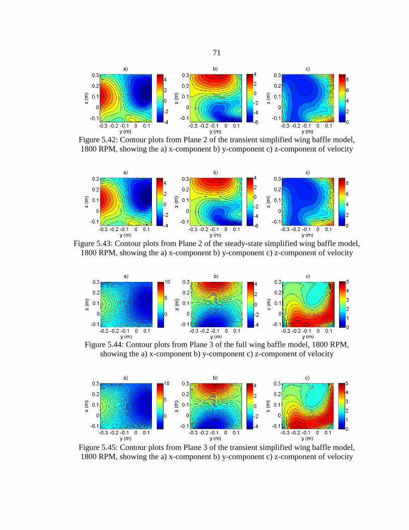
71
Figure 5.42: Contour plots from Plane 2 of the transient simplified wing baffle model,
1800 RPM, showing the a) x-component b) y-component c) z-component of velocity
Figure 5.43: Contour plots from Plane 2 of the steady-state simplified wing baffle model,
1800 RPM, showing the a) x-component b) y-component c) z-component of velocity
Figure 5.44: Contour plots from Plane 3 of the full wing baffle model, 1800 RPM,
showing the a) x-component b) y-component c) z-component of velocity
Figure 5.45: Contour plots from Plane 3 of the transient simplified wing baffle model,
1800 RPM, showing the a) x-component b) y-component c) z-component of velocity

72
Figure 5.46: Contour plots from Plane 3 of the steady-state simplified wing baffle model,
1800 RPM, showing the a) x-component b) y-component c) z-component of velocity
Simplified AHU
All CFD models from this point on utilized the simplified AHU model (Figure 4.2)
with a steady-state flow assumption to solve for the flow structure. This allowed for two
additional baffle types to be quickly modeled to show the effects had on the downstream
flow regime. These two baffles were both perforated plate type flow conditioners which
were designed to straighten the airflow. Streamlines of the velocity flow path in each
model can be seen below, and were used to visually compare the flow profile between the
base AHU, the wing baffle, and both perforated plates. The flow structure from the base
AHU model (Figure 5.47(a)) shows a highly rotational flow which eventually dissipates
part way through the flex duct towards the outlet of the model. Figure 5.47(b) shows the
rotational flow profile created by the wing baffle AHU model, which appears to dissipate
at a much quicker rate than the baseline model. Figure 5.48(a) shows a slightly helical flow
structure created by the first perforated plate (Figure 4.4), although the majority of the
velocity is traveling at a much quicker rate in the downstream direction. Finally, the second
perforated plate (Figure 4.5) creates a completely straightened flow with any turbulence
being dissipated as it traveled through the plate.

73
Figure 5.47: Streamlines for a) base AHU model b) wing baffle model, 1000 RPM
Figure 5.48: Streamlines for AHU model, 1000 RPM with a) perforated plate 1
b) perforated plate 2

74
Assessing Performance
While streamlines and contour plots provide a good visual of the flow structure, it
was desirable to quantitatively characterize the flow uniformity, turbulence levels, and the
amount of rotation in the flow to better compare data between the four different AHU
models. This section will review the calculations from these models to better understand
the effects had on the downstream flow regime, followed by the effects had on the heating
transfer performance through the heating coil region. Values assessed include the RRMSE,
and planar averaged values for flow uniformity, TKE, turbulence intensity, Vorticity,
Helicity, the Q-criterion, and the λ2-criterion.
Flow Characteristics
As previously stated, the flow uniformity is considered to effect the overall
performance of a heat exchanger inside an AHU [3]. The uniformity of the flow was
evaluated at Planes 1, 2 and 3 using the methods previously discussed in the background
and methodology sections as the assessment criterion. Tables 5.1 through 5.3 show the
RRMSE, uniformity, turbulence kinetic energy, and turbulence intensity values as an
average value of all the cells seen across Planes 1, 2, and 3 for a fan speed of 1000 RPM
for the AHU models without and with a baffle. While Plane 1 is the inlet for the simplified
AHU, the values shown in Table 5.1 vary from the boundary conditions. This is due to the
averaging within the first layer of cells at the of inlet, combining the inlet values those of
the flow recirculating due to interactions with the duct walls and the close proximity to any
of the baffles that have been added into the simulation.

75
RRMSE values for the z-component of velocity across Plane 1 show an increased
value when each of the baffles are installed, coinciding with a decrease in the overall
uniformity values. However, RRMSE values for the lateral velocity components show an
increase with the addition of the wing baffle into the system, and a decrease with the
addition of either of the perforated plates. For Planes 2 and 3, The RRMSE values for the
x-component of velocity appear to decrease with the addition of a baffle, whereas the
RRMSE values for the y-component of velocity appear to increase. When observing the z-
component values, a decrease is seen when either the wing baffle or the second perforated
plate is installed, while an increase is seen with the first perforated plate. While there
appears to be no consistent pattern between RRMSE values and the addition of each baffle,
all cases show that the addition of each selected baffle increased the overall flow uniformity
across both Planes 2 and 3 relative to base values. Out of all three baffle types, the second
perforated plate showed the largest increase in uniformity, with a 36% improvement across
Plane 2 and a 30.1% improvement across Plane 3 relative to baseline AHU values. The
wing baffle came last in this category, although is still managed to increase the flow
uniformity by 12% across Plane 2 and by 12.9% across Plane 3 relative to base values.
Observation of the TKE and TI values show that the wing baffle actually increases the
turbulence energy and level of the flow, while both perforated plates drastically decreased
the turbulence levels of the flow downstream of their location. While this decrease was
expected from the perforated plates as they are designed to straighten the flow, the increase
in turbulence levels caused by the wing baffle was not anticipated. This rise of turbulent
energy could potentially accelerate the mixing process within the flow and increase the
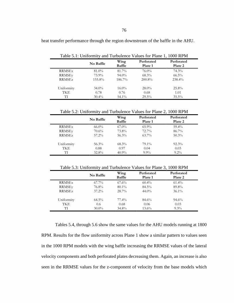
76
heat transfer performance through the region downstream of the baffle in the AHU.
Table 5.1: Uniformity and Turbulence Values for Plane 1, 1000 RPM
No Baffle
Wing Baffle
Perforated Plate 1
Perforated Plate 2
RRMSEx 81.0% 81.7% 76.0% 74.3% RRMSEy 73.9% 94.0% 68.3% 66.5% RRMSEz 155.8% 186.7% 200.8% 238.4%
Uniformity 34.0% 16.0% 28.0% 25.8%
TKE 0.78 0.76 0.68 1.01 TI 30.4% 54.1% 29.5% 35.5%
Table 5.2: Uniformity and Turbulence Values for Plane 2, 1000 RPM
No Baffle
Wing Baffle
Perforated Plate 1
Perforated Plate 2
RRMSEx 66.0% 67.0% 65.9% 59.4% RRMSEy 70.6% 73.8% 72.7% 86.7% RRMSEz 57.2% 56.3% 63.7% 50.3%
Uniformity 56.3% 68.3% 79.1% 92.3%
TKE 0.88 0.97 0.04 0.03 TI 32.8% 40.9% 9.9% 9.2%
Table 5.3: Uniformity and Turbulence Values for Plane 3, 1000 RPM
No Baffle
Wing Baffle
Perforated Plate 1
Perforated Plate 2
RRMSEx 67.7% 67.6% 60.4% 61.4% RRMSEy 76.8% 80.1% 84.5% 89.8% RRMSEz 37.2% 28.7% 44.0% 36.1%
Uniformity 64.5% 77.4% 84.6% 94.6%
TKE 0.6 0.68 0.06 0.03 TI 30.0% 34.8% 13.6% 9.3%
Tables 5.4, through 5.6 show the same values for the AHU models running at 1800
RPM. Results for the flow uniformity across Plane 1 show a similar pattern to values seen
in the 1000 RPM models with the wing baffle increasing the RRMSE values of the lateral
velocity components and both perforated plates decreasing them. Again, an increase is also
seen in the RRMSE values for the z-component of velocity from the base models which

77
correlates well with the decrease in the flow uniformity with the addition of each baffle.
Observing the RRMSE values across Planes 2 and 3, however, shows a slightly different
pattern than seen in the simulations run at 1000 RPM. The wing baffle and first perforated
plate demonstrate an increase for all three velocity components across Plane 2. Although
RRMSE values indicate that the faster blower speed may increase the variance in fluid flow
at each plane, flow uniformity values from both Planes 2 and 3 still show that each baffle
actually increases the uniformity of the flow. This increase in RRMSE values can
potentially be influenced by geometric changes near where the data was taken from. As
can be seen in Figure 4.3, Planes 1 and 2 are located near the downstream side of a
reduction in the AHU geometry, and velocity values across these planes are still trying to
recover from a sudden shift in direction. It is seen once more that both perforated plates
drastically reduce turbulence levels relative to baseline data. The wing baffle still produces
higher turbulence intensity levels than the other models across Planes 1 and 2, although
TKE values decreased by 12-27% when compared with baseline data. By the time the flow
reaches Plane 3, turbulence values drop to just below baseline values. Although the wing
baffle shows elevated turbulence levels relative to baseline values, further observation of
the data shows that these levels drop as the flow travels from Plane 2 to Plane 3, unlike the
baseline values which shows an increase in turbulence from Plane 2 to Plane 3.
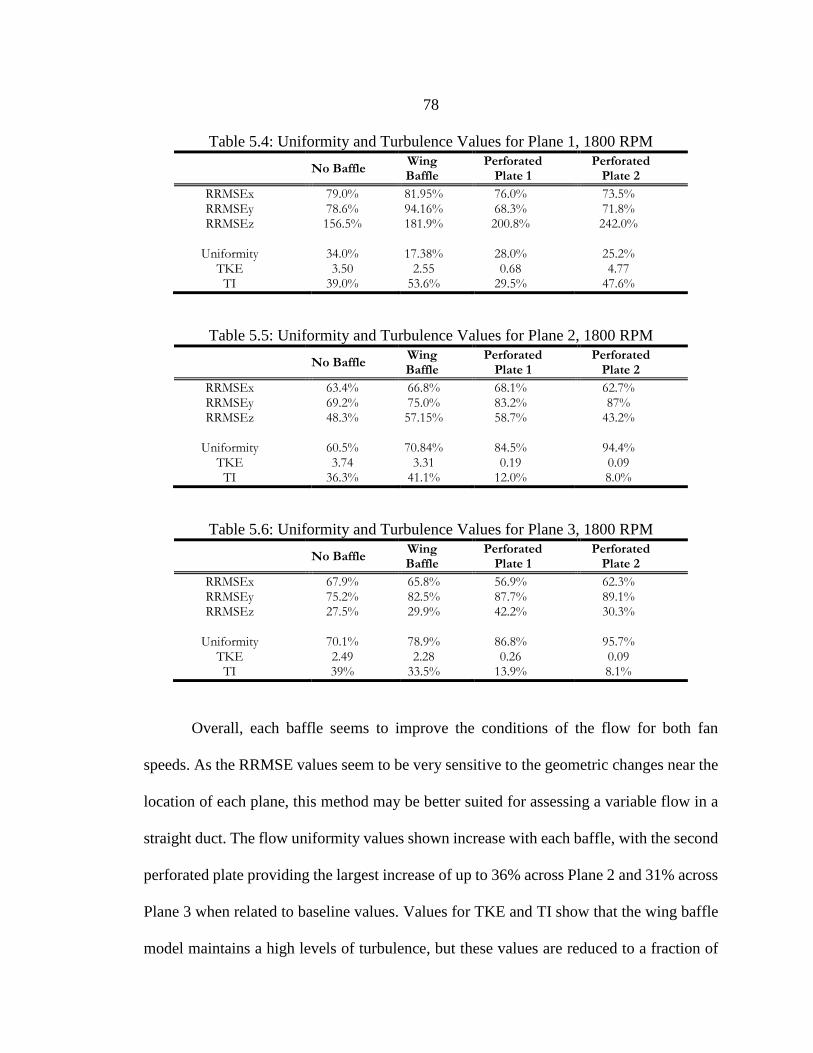
78
Table 5.4: Uniformity and Turbulence Values for Plane 1, 1800 RPM
No Baffle
Wing Baffle
Perforated Plate 1
Perforated Plate 2
RRMSEx 79.0% 81.95% 76.0% 73.5% RRMSEy 78.6% 94.16% 68.3% 71.8% RRMSEz 156.5% 181.9% 200.8% 242.0%
Uniformity 34.0% 17.38% 28.0% 25.2%
TKE 3.50 2.55 0.68 4.77 TI 39.0% 53.6% 29.5% 47.6%
Table 5.5: Uniformity and Turbulence Values for Plane 2, 1800 RPM
No Baffle
Wing Baffle
Perforated Plate 1
Perforated Plate 2
RRMSEx 63.4% 66.8% 68.1% 62.7% RRMSEy 69.2% 75.0% 83.2% 87% RRMSEz 48.3% 57.15% 58.7% 43.2%
Uniformity 60.5% 70.84% 84.5% 94.4%
TKE 3.74 3.31 0.19 0.09 TI 36.3% 41.1% 12.0% 8.0%
Table 5.6: Uniformity and Turbulence Values for Plane 3, 1800 RPM
No Baffle
Wing Baffle
Perforated Plate 1
Perforated Plate 2
RRMSEx 67.9% 65.8% 56.9% 62.3% RRMSEy 75.2% 82.5% 87.7% 89.1% RRMSEz 27.5% 29.9% 42.2% 30.3%
Uniformity 70.1% 78.9% 86.8% 95.7%
TKE 2.49 2.28 0.26 0.09 TI 39% 33.5% 13.9% 8.1%
Overall, each baffle seems to improve the conditions of the flow for both fan
speeds. As the RRMSE values seem to be very sensitive to the geometric changes near the
location of each plane, this method may be better suited for assessing a variable flow in a
straight duct. The flow uniformity values shown increase with each baffle, with the second
perforated plate providing the largest increase of up to 36% across Plane 2 and 31% across
Plane 3 when related to baseline values. Values for TKE and TI show that the wing baffle
model maintains a high levels of turbulence, but these values are reduced to a fraction of
79
the baseline values in both perforated plate models. Although the wing baffle only
increased uniformity by 8-13% relative to the base AHU model, the higher turbulent kinetic
energy and turbulence intensity values may provide desirable a flow structure for heat
transfer than the straight flow produced by either perforated plate.
Different than direct evaluations of the velocity vectors and magnitudes, Tables 5.7
through 5.9 show the vorticity data from all three planes for the 1000 RPM fan speed,
including the vorticity magnitude, vorticity component values, helicity, λ2-criterion, and
Q-criterion values. The vorticity values from Planes 2 and 3 show a more consistent decline
with the addition of each baffle, specifically with the magnitude and z-components. While
the wing baffle does decrease the downstream vorticity magnitude slightly, the first
perforated plate decreases the magnitude by approximately 33%-42% and the second
perforated plate by more than 57% relative to baseline values. Further observation shows
that both perforated plates cause an even larger decrease in the z-component of vorticity
when compared to the AHU model without a baffle. As the measure of the amount of swirl
in the fluid flow, helicity is the dot product between the velocity and the vorticity. Both the
helicity and vorticity directions can be depicted by either a negative or positive sign value,
which can be linked to the common practice of using the right hand rule for rotation to
determine direction. For the simulations with no baffle, the first perforated plate, and the
second perforated plate, the average helicity magnitude consistently shows a decrease
between from Plane 1 to both 2 and 3. The addition of the wing baffle, however, shows a
decrease in the helicity magnitude between Planes 1 and 2, but a noticeable increase
between Planes 2 and 3. This may be a result of the higher turbulence values produced by

80
the wing baffle, creating more kinetic energy in the flow which then reacts with shear
stresses along the walls.
Observation of the λ2-criterion and Q-criterion values indicate a different flow
regime compared to the helicity and vorticity values. As stated in the methodology section
of this thesis, for vorticity to be present, the λ2-criterion should be a negative value
designating a low pressure while Q > 0 suggests that the flow is vorticity dominated. As
averages across each plane, the baseline value of λ2 across Plane 2 was the only value that
suggested a low-pressure core dominated the flow, which is required for a vortex core to
be present. Q-criterion values also specify that the flow across both Planes 2 and 3 for all
of the AHU cases without and with a baffle is predominately strain-based. Further
investigation shows that highly negative λ2 as well as positive Q-criterion values are seen
in the central area of Planes 2 and 3 for the baseline and wing baffle model, indicating that
there are vortex cores of varying magnitudes present for all cases, but not dominating the
flow structure of the whole duct. Along the duct walls on Planes 2 and 3 there exists
sufficiently large values for the λ2 and Q-criterion that suggest a vortex core is not present.
This is possibly due to the shear effects occurring closely along the walls, and may partially
explain why the overall average values would indicate that a vortex core is not present.
Table 5.7: Vorticity Values for Plane 1, 1000 RPM
No Baffle
Wing Baffle
Perforated Plate 1
Perforated Plate 2
Vorticity 28.9 41.59 38.7 58.62 Vorticity (x) 1.71 0.9 5.43 11.58 Vorticity (y) 0.62 1.29 5.38 -1.94 Vorticity (z) 5 3.01 6.87 7.44
Helicity -23.31 -16.08 -41.8 -69.35
λ2-Criterion 8.47 45.49 -202.61 -414.1
Q-Criterion -39.0 -180.37 193.7 416.57

81
Table 5.8: Vorticity Values for Plane 2, 1000 RPM
No Baffle
Wing Baffle
Perforated Plate 1
Perforated Plate 2
Vorticity 29.45 27.14 17.02 12.42 Vorticity (x) -1.51 -4.66 2.04 1.5 Vorticity (y) 0.47 0.84 -1.39 -0.49 Vorticity (z) 11.57 7 3 0.11
Helicity -5.41 3.66 3 -1.5
λ2-Criterion 68.18 184.1 68.42 21.94
Q-Criterion -147.99 -321.58 -11.59 -32.47
Table 5.9: Vorticity Values for Plane 3, 1000 RPM
No Baffle
Wing Baffle
Perforated Plate 1
Perforated Plate 2
Vorticity 29 24.75 19.34 12.4 Vorticity (x) -0.05 -0.74 -0.06 -0.97 Vorticity (y) 1.35 0.77 -2.09 -0.38 Vorticity (z) 9.9 4.12 1.38 0.16
Helicity 2.67 11.02 3.39 -0.38
λ2-Criterion -28.74 22.59 38.29 31.97
Q-Criterion -15.23 -57.36 -58.03 -44.89
Average vorticity values across Planes 2 and 3 for a fan speed of 1800 RPM also
indicate that the addition of any of the baffles helps to dissipate the vortex core at a quicker
rate. Vorticity values from the wing baffle simulation show a consistent decrease between
Planes 1 and 3, while vortex dissipation in both of the perforated plate AHU models appears
to occur more instantaneously due to their flow conditioning nature. A drastic decrease in
helicity magnitudes is again seen between Plane 1 to Planes 2 and 3 for the base AHU and
both perforated plate models (Tables 5.10 through 5.12) at this fan speed. Helicity values
for the wing baffle model again show a noticeable increase between Planes 2 and 3, which
may be due to any secondary flow (minor flows superimposed onto the primary flow)
caused by the wing baffle.
Q and λ2-criterion values maintain a similar pattern to what is seen from the 1000
RPM AHU models, with a very localized vortex core in the baseline and wing baffle AHU

82
models. The shear stress acting on the fluid along the wall surface produces large values
for Q and λ2 that indicate a vortex core does not occur when looking at the average planar
values.
Table 5.10: Vorticity Values for Plane 1, 1800 RPM
No Baffle
Wing Baffle
Perforated Plate 1
Perforated Plate 2
Vorticity 56.92 76.01 77.58 120.79 Vorticity (x) 1.99 2.54 13.83 29.13 Vorticity (y) 4.61 3.29 12.07 0.2 Vorticity (z) 10.37 7.11 12.94 13.44
Helicity -96.2 -40.33 -164.6 -268.2
λ2-Criterion -1.49 201.45 -896.32 -1724.6
Q-Criterion -96.4 -676.47 876.82 1822
Table 5.11: Vorticity Values for Plane 2, 1800 RPM
No Baffle
Wing Baffle
Perforated Plate 1
Perforated Plate 2
Vorticity 45.85 48.58 28.38 20.79 Vorticity (x) -1.79 -9.28 2.94 2.51 Vorticity (y) 0.355 -1.04 -2.04 -0.98 Vorticity (z) 23.85 14.09 5.46 0.154
Helicity 21.44 17.03 6.23 -6.00
λ2-Criterion 256.6 835.45 250.1 118.35
Q-Criterion -567.16 -1414 -403.78 -163.12
Table 5.12: Vorticity Values for Plane 3, 1800 RPM
No Baffle
Wing Baffle
Perforated Plate 1
Perforated Plate 2
Vorticity 43.19 39.3 31.69 20.77 Vorticity (x) 0.5 0.39 -1.66 -0.61 Vorticity (y) 3.99 2.03 -4.05 -0.57 Vorticity (z) 22.31 12.35 2.7 0.52
Helicity 49.81 50.44 9.53 -1.8
λ2-Criterion -84.25 67.17 152.87 125.51
Q-Criterion -24.04 -170.35 -215.66 -167.95
Overall, a visual comparison, as quantification of the simulated results,
demonstrates that the addition of a baffle to the AHU shows a definitive change in the flow
structure and overall improved uniformity. Further investigation shows that the perforated

83
plates increased the uniformity the most by acting as flow straighteners and greatly
reducing the vorticity of the flow; with the wing baffle showing the least amount of
improvement (9-13% improvement in flow uniformity relative to base values), but
managing to conserve or increase the inflow turbulence levels and the rotational energy.
Heating Coil
The addition of a heating coil into the model allowed heat transfer to be assessed
relative to differences in the flow structure without and with baffles. A heat transfer rate of
15 kW was added into the simplified AHU models. Table 5.13 shows the heat transfer
values for the heating coil when the inertial and viscous resistance coefficients are included
and the percent change in heat exchanger performance caused by each baffle versus the
baseline values. Table 5.14 shows the same data, but for the heating coil region set as
completely open, i.e. the pressure resistance coefficients are set to 0. It is important to
reiterate that the values for heat transfer are shown in order to provide the predicted effects
of adding a baffle into an AHU system and that they have not been compared against
experimental data. While not verified for heat transfer, the models without the heating coil
compared well to the experiments and should be representative of expected data for the
new models. Therefore, these values should be able to provide initial insight into the
strength and weakness of each baffle when used inside this particular AHU geometry.
Observation of the heat transfer values shows that the addition of a baffle does not
dependably increase or decrease the heat exchanger performance, even though all the
baffles improved flow uniformity. The addition of the wing baffle into the flow appears to
increase the heat transfer from baseline values for 75% of the cases shown, with the case

84
utilizing the pressure resistance coefficients at a blower speed of 1800 rpm remaining
nearly unchanged compared to the baseline. Both perforated plates show a pattern of
decreasing heat exchanger performance in most of the cases. More so, in the two instances
where more than one of the baffles managed to increase the total heat transfer through the
system, the wing baffle still provided are larger increase.
Table 5.13: Heat transfer rate with pressure resistance coefficients
No Baffle
Wing Baffle
Perforated Plate 1
Perforated Plate 2
1000 RPM Heat Transfer (W) 16341.07 16454.25 16430.66 16291.02
% Performance Change 0.69% 0.55% -0.31%
1800 RPM Heat Transfer (W) 16962.91 16934.32 16944.64 16819.57 % Performance Change -0.17% -0.11% -0.85%
Table 5.14: Heat transfer rate, no pressure resistance coefficients
No Baffle
Wing Baffle
Perforated Plate 1
Perforated Plate 2
1000 RPM Heat Transfer (W) 18993.31 19033.34 18826.96 18815.03
% Performance Change 0.21% -0.88% -0.94%
1800 RPM Heat Transfer (W) 16333.43 16616.44 16315.89 16466.29 % Performance Change 1.73% -0.11% 0.81%
The simulations where the heating coil had no pressure losses had a negligible
impact on the flow characteristics. Uniformity values across Plane 2 appear to stay very
similar to values seen without the heating coil included, while uniformity data from Plane
3 for all of the simulations indicates that downstream flow becomes increasingly uniform
as it passes through the heating coil; essentially, the porous medium acts as a flow
straightener, even with isotropic pressure loss characteristics, and the flow data across all
simulations contains very little variance when compared. At Plane 3 though, the x-
component of velocity shows very little change in flow uniformity and the y-component
85
shows a large increase in non-uniformity compared to results from the CFD models where
the heating coil region was omitted. This can be explained by the location of Plane 3, which
is located directly along a shift in the duct size along the y axis. As the lateral velocity-
components are nearly zero across the majority of Plane 3, this slight shift in geometry is
enough to create what appears as a large variance occurring along the walls and a large
increase in flow non-uniformity. The location of Plane 3 was chosen to match where the
experimental data was taken. Future studies should, where possible, measure further away
from changes in the geometry which may include any include any seams or lips between
pieces of sheet metal.
The addition of the heating coil with the pressure resistance coefficients appears to
reduce the overall turbulence of the flow. These values are shown in Tables 5.15 through
5.20. Comparing results between the all of the AHU models with this porous heating coil
region show a variety of changes in the RRMSE values, but again show no pattern
suggesting they have a direct connection with the actual uniformity of the flow. A similar
pattern from before does emerge regarding the expected turbulence levels downstream of
each baffle, mainly that the wing baffle again produces larger turbulence levels than either
perforated plates do, although the turbulence levels appear to be reduced when compared
to the CFD models with the heating coil region omitted.

86
Table 5.15: Uniformity and turbulence values for Plane 1, 1000 RPM
No Baffle
Wing Baffle
Perforated Plate 1
Perforated Plate 2
RRMSEx 76.1% 73.8% 76.2% 76.1% RRMSEy 68.5% 70.1% 68.5% 68.6% RRMSEz 195.6% 206.5% 195.4% 195.6%
Uniformity 28.2% 28.4% 28.3% 28.2%
TKE 3.09 4.16 0.71 1 TI 67.6% 44.4% 30.2 35.0%
Table 5.16: Uniformity and turbulence values for Plane 2, 1000 RPM
No Baffle
Wing Baffle
Perforated Plate 1
Perforated Plate 2
RRMSEx 70.9% 63.7% 63.2% 61.1% RRMSEy 69.3% 70.6% 64.4% 60.2% RRMSEz 26.1% 30.6% 41.4% 29.47%
Uniformity 63.2% 67.4% 79.5% 91.5%
TKE 1.28 0.70 0.09 0.06 TI 35.4% 28.12% 11.3% 11.1%
Table 5.17: Uniformity and turbulence values for Plane 3, 1000 RPM
No Baffle
Wing Baffle
Perforated Plate 1
Perforated Plate 2
RRMSEx 124.5% 122.8% 126.3% 126.2% RRMSEy 71.2% 71.3% 71.3% 71.9% RRMSEz 5.1% 4.6% 4.8% 5.1%
Uniformity 99.2% 99.1% 99.2% 99.2%
TKE 0 0.01 0 0.01 TI 2.2% 1.9% 2.2% 2.2%
Table 5.18: Uniformity and turbulence values for Plane 1, 1800 RPM
No Baffle
Wing Baffle
Perforated Plate 1
Perforated Plate 2
RRMSEx 75.0% 73.8% 75.0% 75.0% RRMSEy 73.2% 70.1% 73.3% 73.3 RRMSEz 197.1% 206.5% 197.0% 197.0%
Uniformity 28.1% 28.4% 28% 28.1%
TKE 3.6 4.16 3.22 4.75 TI 42.0% 44.4% 38.6% 46.4%

87
Table 5.19: Uniformity and turbulence values for Plane 2, 1800 RPM
No Baffle
Wing Baffle
Perforated Plate 1
Perforated Plate 2
RRMSEx 66.4% 62.5% 64.3% 60.4% RRMSEy 68.2% 68.3% 68.7% 60.5% RRMSEz 32.8% 30.9% 40.5% 28.4%
Uniformity 62.7% 71.6% 83% 93.0%
TKE 3.57 2.89 0.44 0.21 TI 29.8% 31.6% 13.9% 10.9%
Table 5.20: Uniformity and turbulence values for Plane 3, 1800 RPM
No Baffle
Wing Baffle
Perforated Plate 1
Perforated Plate 2
RRMSEx 123.2% 122.8% 125.4% 125.3% RRMSEy 72.7% 71.3% 72.3% 73.2% RRMSEz 4.6% 4.6% 4.3% 4.5%
Uniformity 99.2% 99.1% 99.2% 99.2%
TKE 0.01 0.01 0.01 0.01 TI 1.9% 1.9% 1.8% 1.9%
Helicity and vorticity values across Planes 2 and 3 (Tables 5.21 -5.26) show very
similar patterns between all 4 models which indicate that the addition of a heating coil into
the system affects the upstream and downstream flows surrounding it. Similar to the 1000
RPM models, the planar averaged Q and λ2-Criterion values continue to indicate that
vortices do not exist in the flow. Visualizing the velocity data via scalar plots shows that
these values also appear to be accurate in this case as the flow is highly uniform and
unidirectional due to the flow straightening effect from the heating coil region.

88
Table 5.21: Vorticity values for Plane 1, 1000 RPM
No Baffle
Wing Baffle
Perforated Plate 1
Perforated Plate 2
Vorticity 31.94 65.5 43.6 63.79 Vorticity (x) 1.43 -8.93 4.9 13.59 Vorticity (y) 4.62 7.05 5.42 -40.07 Vorticity (z) 6.78 6.25 6.74 6.70
Helicity -26.1 -19.78 -40.18 -70.79
λ2-Criterion -34.7 171.59 -186.68 -414.88
Q-Criterion -9.93 -379.12 165.25 414.11
Table 5.22: Vorticity values for Plane 2, 1000 RPM
No Baffle
Wing Baffle
Perforated Plate 1
Perforated Plate 2
Vorticity 23.48 26.46 26.57 22.00 Vorticity (x) -0.66 -0.03 -0.624 0.76 Vorticity (y) -0.53 -0.81 -2.15 -1.21 Vorticity (z) 9.88 5.98 2.6 0.21
Helicity 20.77 5.06 6.16 -1.30
λ2-Criterion 115.91 90.16 113.81 18.73
Q-Criterion -197.05 -156.85 -210.35 -46.4
Table 5.23: Vorticity values for Plane 3, 1000 RPM
No Baffle
Wing Baffle
Perforated Plate 1
Perforated Plate 2
Vorticity 4.972 5.27 4.56 5.046 Vorticity (x) 0.092 0.181 0.069 0.18 Vorticity (y) 0.29 0.297 0.407 0.236 Vorticity (z) -0.003 0.003 0.001 0.0
Helicity -0.007 -0.011 -0.005 -0.013
λ2-Criterion 41.91 42.23 41.25 42.21
Q-Criterion -4.72 -48.05 -46.09 -46.99
Table 5.24: Vorticity values for Plane 1, 1800 RPM
No Baffle
Wing Baffle
Perforated Plate 1
Perforated Plate 2
Vorticity 55.98 109.93 87.29 134.64 Vorticity (x) 5.18 -13.4 16.15 35.28 Vorticity (y) 4.55 11.38 12.32 -1.65 Vorticity (z) 12.68 10.76 12.69 12.63
Helicity -94.31 -78.4 -175.55 -290.53
λ2-Criterion -2.19 363.8 -844.5 -1745.8
Q-Criterion -200 -930.1 832.68 1853.4

89
Table 5.25: Vorticity values for Plane 2, 1800 RPM
No Baffle
Wing Baffle
Perforated Plate 1
Perforated Plate 2
Vorticity 48.91 41.61 42.26 36.77 Vorticity (x) -0.82 -1.74 -0.97 0.84 Vorticity (y) 0.31 -2.0 -2.87 -2.29 Vorticity (z) 15.84 13.32 5.02 -0.24
Helicity 36.3 38.1 14.14 -0.07
λ2-Criterion 498.23 398.2 520.94 127.37
Q-Criterion -840.45 -653.7 -898.94 -244.6
Table 5.26: Vorticity values for Plane 3, 1800 RPM
No Baffle
Wing Baffle
Perforated Plate 1
Perforated Plate 2
Vorticity 7.38 7.7 6.72 7.42 Vorticity (x) 0.2 0.3 0.12 0.26 Vorticity (y) 0.52 0.44 0.61 0.38 Vorticity (z) 0.002 0.01 0.01 -0.01
Helicity -0.005 -0.01 0.0063 -0.06
λ2-Criterion 146.41 148.64 143.04 147
Q-Criterion -162.4 -164.3 -157.04 -160.65
Based on the data shown in this section, it is believed that the wing baffle is the
only baffle reviewed that may effectively help increase the overall heat exchanger
performance in this AHU geometry. In 75% of the cases observed it managed to increase
the heat exchanger performance by the highest amount. In the one case which showed
otherwise (1800 RPM with resistance coefficients), the turbulence level was lower than the
simulation the pressure loss characteristics. While both perforated plate baffles managed
to consistently increase the downstream flow uniformity, they provided the least favorable
heat transfer values as well as the lowest downstream turbulence and vorticity levels. This
suggests that there may be an optimum flow uniformity to TKE ratio in which a baffle may
increase the overall heat exchanger performance in this specific geometry. A more in depth
study is required to fully understand the significant effects of different baffle types on the
heat exchanger performance within an AHU system.

90
6 CONCLUSION
This study was conducted to determine if there was an effective way for HVAC
manufacturers to characterize the airflow through an AHU system without having to build
a physical model for every design iteration, reducing the overall cost and material use of
the design process. In the past, much of the research conducted has been focused on isolated
components such as heat exchangers or blower units. This is useful for determining ideal
operating conditions; however much of that research does not take into account real world
scenarios that combine the heating coil, blower unit, and a cooling coil within an AHU.
The research presented in this thesis used computational fluid dynamics to model the
airflow through an AHU in order to understand the flow uniformity and its impact on heat
transfer, taking into account components normally found in an AHU system. A porous
region was used as a surrogate to the real geometry of the cooling coil, where the physical
parameters were calibrated against experiments conducted in the HVAC lab at Montana
State University. These tuned parameters provided the inertial and viscous resistance
coefficients used in the porous continuum. CFD analysis using an unsteady Reynolds-
Averaged Navier Stokes solver was then compared with experimental data.
Comparing the experimental data with numerical values showed a good correlation
for the base AHU models. While downstream-component velocity values are mostly within
the estimated error expected by experimental values, simulated values appear to trend
slightly higher in the center of the flow. Results from the AHU with the wing baffle again
correlate well with experimental data for the lateral-components of velocity; however,
while most of the simulated values show a good correlation for the downstream-component

91
of velocity, experimental data shows that there is an apparent shift in the low end of the
flow range between base and wing baffle AHU models. Unfortunately, there lacks a full
description of the flow profile within the experiments to fully observe this modification in
the flow structure due to limitations of the experimental setup. Both AHU models also
show an overestimation along the walls of the AHU for all velocity components. While the
correlation between experimental data and simulated values proves the usefulness of CFD
as a design tool, future studies should be performed to further investigate the sensitivity of
results in these systems to the particular turbulence model used.
This study also confirmed that it is possible to drastically reduce the required
computational time by omitting the blower unit and switching from a transient to a steady-
state solution. Although the blower induced flow is transient by nature, it was seen that
once a developed flow in the downstream flow regime occurred, the transient velocity
oscillated about an average with a small variance. To demonstrate this, velocity data from
the full AHU models was taken over a range of time, and the linear regression of the
velocity values showed that the change in average velocity along each mesh cell was
insignificant and that a steady state model could potentially replace the transient one. Next,
a simplified AHU model was created, which only contained everything downstream of the
blower and utilized average velocity values from that location as the inlet conditions.
Velocities and turbulence values for transient and steady-state simulations of this
simplified AHU showed a very strong correlation when compared with values from the full
AHU models. This justified the use of the simplified models to observe the change in the
downstream flow characteristics caused by the addition of each baffle. Although in this

92
case a full AHU model was first required to obtain the appropriate inlet velocities and
turbulence conditions, The ability to use a steady-state solution and physically neglect
upstream geometries may allow designers and manufacturers to create a base model for
each unit and then quickly optimize the airflow through it by adding baffles, or making
minor geometric changes to the system.
Velocity, turbulence, and vorticity data were able to show the effects each baffle
had on the system when compared to the baseline AHU model without a baffle. While all
baffles appeared to have increased the overall downstream flow uniformity, with the wing
baffle showing the smallest increase and the second perforated plate showing the largest
increase in uniformity. Although the wing baffle provided the lowest increase in velocity
uniformity, approximately 9-13% relative to base AHU values, it was able to increase the
turbulence by 5-13%. Both of the perforated plates acted as a flow straightener, reducing
the downstream turbulence, helicity, and vorticity levels to a minimum.
With the addition of a heating coil into the system, the wing baffle provided the
largest increase in heat transport compared to baseline values, with a decrease in
performance being seen by all three baffles in the case using a blower speed of 1800 RPM
and prescribed pressure loss in the heating coil. This increase in performance seen by the
wing baffle is possibly related to the combination of increased uniformity over the baseline
with higher turbulence levels, although this is likely to be highly dependent on specific
heating coil parameters, as well as the geometry of the AHU system.
The research presented in this thesis could be expanded in multiple ways. In order
to further validate the turbulence model, simulations using an LES model should be

93
performed and compared to data collected in this study. It would also be useful to collect
experimental data on a grid across multiple planes to obtain a more detailed description of
the real world flow conditions. Any number of baffle geometries can be applied to this
baseline AHU model to achieve a better understanding of what may constitute an optimal
design for improving the quality of the flow and heat transfer. The, evaluation of heat
exchanger performance can be improved upon by obtaining parameters from a real world
heating coil, or even utilizing actual geometries as opposed to a porous region.

94
REFERENCES CITED
[1] "Residential Energy Consumption Survey (RECS)," U.S. Energy Information
Administration, 2009.
[2] "U.S. Energy Information Administration," 3 April 2015. [Online]. Available:
http://www.eia.gov/tools/faqs/faq.cfm?id=86&t=1. [Accessed 1 July 2015].
[3] C. T'Joen, M. De Paepe and F. Vanhee, "HEAT EXCHANGER BEHAVIOUR IN
NON UNIFORM FLOW," Experimental Heat Transfer, pp. 281-296, 2006.
[4] V. A. Jairazbhoy, L. Wang, M. Shahabi, R. Nimbalkar and S. Earla,
"OPTIMIZATION OF AIRFLOW THROUGH A HEAT EXCHANGER IN AN
AUTOMOTIVE HVAC," in 3rd ANSA & μETA International Conference,
Halkidiki, Greece, 2009.
[5] D. Yashar, H. Cho and P. Domanski, "Measurement of Air-Velocity Profiles for
Finned-Tube Heat Exchangers Using Particle Image Velocimetry," in International
Refrigeration and Air Conditioning Conference, West Lafayette, 2008.
[6] X. Cao, J. Liu, N. Jiang and Q. Chen, "Particle Image Velocimetry measurement of
indoor airflow field: A review of the technologies and applications," Energy and
Building, no. 69, pp. 367-380, 2014.
[7] X. Sun, Numerical and Experimental Investigation of Tidal Current Energy
Extraction, Edinburgh: The University of Edinburgh, 2008.
[8] L. Zhao, W. Qiao and L. Ji, "Computational fluid dynamics simulation of sound
propagation through a blade row," Acoustical Sociatey of America, vol. 132, no. 4,
pp. 2210-2217, 2012.
[9] B. Trimoreau, R. S. Lutzen, J. Vindahl Kringelum, A. Shajarati and P. Skjellerup,
"New achievements in underwater noise modelling for offshore pile driving," in
Inter-noise, Melbourne, 2014.
[10] C. A. Balaras, E. Dascalaki and A. Gaglia, "HVAC and indoor thermal conditions
in hospital operating rooms," Energy and Buildings, vol. 39, no. 4, pp. 454-470,
2007.

95
[11] W. A. Abdelmaksoud, H. E. Khalifa and T. Q. Dang, "IMPROVED CFD
MODELING OF A SMALL DATA CENTER TEST CELL," in IEEE, Las Vegas,
2010.
[12] S. Knudsen, G. L. Morrison, M. Behnia and S. Furbo, "Analysis of the flow
structure and heat transfer in a vertical mantle heat exchanger," Solar Energy, pp.
281-289, 2005.
[13] K. K. Patel and P. M. Patel, "PERFORMANCE IMPROVEMENT OF
CENTRIFUGAL FAN BY USING CFD," International Journal of Advanced
Engineering Research and Studies, vol. II, no. II, pp. 1-4, 2013.
[14] "HVAC," 28 June 2015. [Online]. Available: https://en.wikipedia.org/wiki/HVAC.
[15] Fundamentals of HVAC Systems, ASHRAE Self-Directed Learning, 2008.
[16] "Questions About Your Community: Indoor Air," United States Environmental
Protection Agency, 8 October 2015. [Online]. Available:
http://www.epa.gov/region1/communities/indoorair.html. [Accessed October 2015].
[17] C.-P. Chio and C.-M. Liao, "Assessment of atmospheric ultrafine carbon particle-
induced human health risk based on surface area dosimetry," Atmospheric
Environment, pp. 8575-8584, 2008.
[18] ASHRAE, "Top Ten Things About Air Conditioning," [Online]. Available:
https://www.ashrae.org/resources--publications/free-resources/top-ten-things-about-
air-conditioning#4. [Accessed 18 May 2015].
[19] L. Morawska, V. Agranovski, Z. Ristovski and M. Jamriska, "Effect of Face
Velocity and the Nature of Aerosol on the Collection of Submicrometer Particules
by Electrostatic Precipitator," Blackwell Publishing, Brisbane, Australia, 2002.
[20] J. Deane, "Conditioning flow disturbances for precision flow metering," Instrument
& Control Systems, San Marcos, CA, 1996.
[21] Y. A. El Drainy, K. M. Saqr, H. S. Aly and M. N. M. Jaafar, "CFD ANALYSIS OF
INCOMPRESSIBLE TURBULENT SWIRLING FLOW THROUGH ZANKER
PLATE," Engineering Applications of Computational Fluid Mechanics, pp. 562-
572, 2009.
96
[22] A. Erdal, "A numerical investigation of different parameters that affect the
performance of a flow conditioner," Flow Measurement and Instrumentation, vol.
8, no. 2, pp. 93-102, 1998.
[23] "Value in the Air, Why Direct Drive Backward Curved Plenum Fans?," AAON,
Inc., Tulsa, OK.
[24] Raunekk, "Types of Heat Exchangers Used in HVAC Systems," Bright Hub
Engineering, 9 March 2009. [Online]. Available:
http://www.brighthubengineering.com/hvac/28623-types-of-heat-exchangers-used-
in-hvac-systems/#. [Accessed 2015].
[25] P. Wais, "Fin-Tube Heat Exchanger Optimization," in Heat Exchangers - Basic
Design Applications, InTech, 2012, pp. 343-366.
[26] O. Zikanov, Essential Computational Fluid Dynamics, Hoboken: John Wiley &
Sons, Inc., 2010.
[27] S. Jain and Y. Deshpande, "CFD Modeling of a Radiator Axial Fan for Air Flow
Distribution," International Science Index Vol: 6, No: 11, pp. 1054 - 1059, 2012.
[28] S. Chaudhary and S. Kansal, "Performance Analysis of Backward Curved
Centrifugal Fan in Heating Ventilation and Air Conditioning," International
Journal of Science and Research Vol: 2, No: 6, pp. 170-172 , 2013.
[29] P. C. Atre and K. R. R. Thundil, "Numerical Design and Parametric Optimization
of Centrifugal Fans with Airfoil Blade Impellers," Research Journal of Recent
Sciences, Vol: 1, pp. 7-11, 2012.
[30] O. P. Singh, R. Khilwani, T. Sreenivasulu and M. Kannan, "PARAMETRIC
STUDY OF CENTRIFUGAL FAN PERFORMANCE: EXPERIMENTS AND
NUMERICAL SIMULATION," International Journal of Advances in Engineering
& Technology, pp. 33-50, 2011.
[31] M. M. A. Bhutta, N. Hayat, M. H. Bashir, A. R. Kahn, K. N. Ahmad and S. Kahn,
"CFD Applications in various heat exchangers design: A review," Applied Thermal
Engineering, pp. 1-12, 2012.
97
[32] S. K. Ramachandran, NUMERICAL ANALYSIS OF AIRSIDE CHARACTERISTICS
IN PLAIN AND WAVY HEAT EXCHANGERS IN THE TURBULENT FLOW
REGIME, Bozeman, MT: Montana State University, 2010.
[33] K. Kritikos, C. Albanakis, D. Missirlis, Z. Vlahostergios, A. Goulas and P. Storm,
"Investigation of the thermal efficiency of a staggered elliptic-tube heat exchanger
for aeroengine applications," Applied Thermal Engineering, 2009.
[34] A. M. Hayes, J. A. Kahn, A. H. Shaaban and I. G. Spearing, "The thermal modeling
of a matrix heat exchanger using a porous medium and the thermal non-equilibrium
model," International Journal of Thernal Sciences, pp. 1-10, 2007.
[35] Z. Zang and Y. Li, "CFD simulation on inlet configuration of plate-fin heat
exchangers," Science Direct, pp. 673-678, 2003.
[36] J. Wen and Y. Li, "Study of flow distribution and its improvement on the header of
plate-fin heat exchanger," Science Direct, pp. 823-831, 2004.
[37] Z. Feng, Z. Long and Q. Chen, "Assessment of various CFD models for predicting
airflow and pressure drop through pleated filter system," Building and
Environment, pp. 132-141, 2014.
[38] V. Holmen, "Methods for Vortex Identification," 2012.
[39] J. P. Holman, "Heat Transfer," McGraw-Hill, 2002, p. 207.
[40] "Mesh Models in STAR-CCM+," 21 November 2013. [Online]. Available:
http://theansweris27.com/mesh-models-in-starccm/. [Accessed 30 March 2015].
[41] "Introduction to turbulence/Turbulence Kinetic Energy," 13 December 2013.
[Online]. Available: http://www.cfd-
online.com/Wiki/Introduction_to_turbulence/Turbulence_kinetic_energy.
[Accessed 5 April 2015].
[42] "Turbulence Intensity," 3 January 2012. [Online]. Available: http://www.cfd-
online.com/Wiki/Turbulence_intensity. [Accessed 5 April 2015].
[43] G. Haller, "An objective definition of a vortex," Fluid Mechanics, vol. 525, no. 1,
pp. 1-26, 2005.
98
[44] H. K. Moffatt, "Helicity and singular structures in fluid dynamics," Proceedings of
the National Acadamy of Sciences of the United States of America, pp. 3663 - 3670,
2014.
[45] N. G. Deen, B. H. Hjertager and T. Solberg, "Comparison of PIV and LDA
Measurement Methods Applied to the Gas-Liquid Flow in a Bubble Column," in
10th International Symposium on Applications of Laser Techniques to Fluid
Mechanics, Lisbon, Portugal, 2000.
[47] "Wikipedia," 10 January 2015. [Online]. Available:
http://en.wikipedia.org/wiki/Flow_conditioning. [Accessed 20 May 2015].
[48] K. A. Hall, "COMPUTATIONAL FLOW MODEL OF WESTFALL'S LEADING
TAB FLOW CONDITIONER," Alden Research Laboratory, Inc., Holden, MA,
2009.
[49] P. C. Atre and K. R. R. Thundil, "Numerical Design and Parametric Optimization
of Centrifugal Fans with Airfoil Blade Impellers," Research Journal of Recent
Sciences, pp. 7-11, 2012.
[50] A. D. Jadhav and T. A. Koli, "CFD Analysis of Shell and Tube Heat Exchanger to
Study the Effect of Baffle Cut on the Pressure Drop," International Journal of
Research in Aeronautical and Mechanical Engineering, pp. 1-7, 2014.
[51] C. Winters, "What kind of furnace air filter do I need, and how often should I
change it?," Control Tech, November 2014. [Online]. Available:
http://controltech.biz/what-kind-of-furnace-air-filter-do-i-need-and-how-often-
should-i-change-it/. [Accessed September 2015].
[52] "Air Cooled Heat Exchanger for Marine Services," dougleschan.com, 6 February
2015. [Online]. Available: http://dougleschan.com/air-cooled-Heat-Exchanger-
marine-services/photos-of-fin-tubes-and-examples/.