characterizing gld via l-moments

8/7/2019 characterizing GLD via L-moments

http://slidepdf.com/reader/full/characterizing-gld-via-l-moments 1/17

a r X i v : m a t h / 0

7 0 1 4 0 5 v 2

[ m a t h . S

T ] 2 6 J u n 2 0 0 7

Characterizing the generalized lambda

distribution by L-moments

Juha Karvanen ∗

Department of Health Promotion and Chronic Disease Prevention, National Public

Health Institute, Mannerheimintie 166, 00300 Helsinki, Finland

Arto Nuutinen

University of Helsinki, V¨ ain¨ o Auerin katu 1, 00560 Helsinki, Finland

Abstract

The generalized lambda distribution (GLD) is a flexible four parameter distributionwith many practical applications. L-moments of the GLD can be expressed in closedform and are good alternatives for the central moments. The L-moments of the GLDup to an arbitrary order are presented, and a study of L-skewness and L-kurtosisthat can be achieved by the GLD is provided. The boundaries of L-skewness and L-

kurtosis are derived analytically for the symmetric GLD and calculated numericallyfor the GLD in general. Additionally, the contours of L-skewness and L-kurtosis arepresented as functions of the GLD parameters. It is found that with an exceptionof the smallest values of L-kurtosis, the GLD covers all possible pairs of L-skewnessand L-kurtosis and often there are two or more distributions that share the sameL-skewness and the same L-kurtosis. Examples that demonstrate situations wherethere are four GLD members with the same L-skewness and the same L-kurtosis arepresented. The estimation of the GLD parameters is studied in a simulation examplewhere method of L-moments compares favorably to more complicated estimationmethods. The results increase the knowledge on the distributions that belong to theGLD family and can be utilized in model selection and estimation.

Key words: skewness, kurtosis, L-moment ratio diagram, method of moments,method of L-moments

∗ Corresponding author. Tel. +358 9 4744 8641, Fax +358 9 4744 8338Email address: [email protected] (Juha Karvanen).

19 December 2010

http://lanl.arxiv.org/abs/math/0701405v2









































1 Introduction

The generalized lambda distribution (GLD) is a four parameter distribu-tion that has been applied to various problems where a flexible parametric

model for univariate data is needed. The GLD provides fit for a large rangeof skewness and kurtosis values and can approximate many commonly useddistributions such as normal, exponential and uniform. The applications of the GLD include e.g. option pricing (Corrado, 2001), independent componentanalysis (Karvanen et al., 2002), statistical process control (Pal, 2005), anal-ysis of fatigue of materials (Bigerelle et al., 2005), measurement technology(Lampasi et al., 2005) and generation of random variables (Ramberg and Schmeiser,1974; Karvanen, 2003; Headrick and Mugdadib, 2006).

The price for the high flexibility is high complexity. Probability density func-tion (pdf) or cumulative distribution function (cdf) of the GLD do not exist in

closed form but the distribution is defined by the inverse distribution function(Ramberg and Schmeiser, 1974)

F −1(u) = λ1 +uλ3 − (1− u)λ4

λ2

, (1)

where 0 ≤ u ≤ 1 and λ1, λ2, λ3 and λ4 are the parameters of the GLD.Equation (1) defines a distribution if and only if (Karian et al., 1996)

λ2

λ3uλ3−1 + λ4(1

−u)λ4−1

≥ 0 for all u ∈ [0, 1]. (2)

Karian et al. (1996) divide the GLD into six regions on the basis of the param-eters λ3 and λ4 that control skewness and kurtosis of the distribution. Theseregions are presented in Figure 1. The regions have different characteristics:the distributions in region 3 are bounded whereas the distributions in region 4are unbounded; the distributions in regions 1 and 5 are bounded on the rightand the distributions in regions 2 and 6 are bounded on the left. The bound-aries of the domain in each region are described e.g. by Karian and Dudewicz(2000) and Fournier et al. (2007).

The members of the GLD family have been traditionally characterized by

the central moments, especially by the central moment skewness and kurto-sis (Ramberg and Schmeiser, 1974; Karian et al., 1996). L-moments (Hosking,1990), defined as linear combinations of order statistics, are attractive al-ternatives for the central moments. Differently from the central moments,the L-moments of the GLD can be expressed in closed form, which allowsus to derive some analytical results and makes it straightforward to per-form numerical analysis. The parameters of the GLD can be estimated bymethod of L-moments (Karvanen et al., 2002; Asquith, 2007). Method of L-

2



- 3 - 2 - 1 1 2 3

- 3

- 2

- 1

1

2

3

Region3

Region4

Region1

Region2

R e g i o n 5

Region6

not valid

n o t v a l i d

λ4

λ3

Fig. 1. GLD regions as defined in (Karian et al., 1996). The distributions arebounded on the right in regions 1 and 5, bounded on the left in regions 2 and6, bounded in region 3 and unbounded in region 4.

moments can be used independently or together with other estimation meth-ods, analogously to what was done in (Su, 2007), (Fournier et al., 2007) and(Lakhany and Mausser, 2000) with numerical maximum likelihood, methodof moments, method of percentiles (Karian and Dudewicz, 1999), the leastsquare method (Ozturk and Dale, 1985) and the starship method (King and MacGillivray,

1999).

Karian and Dudewicz (2003) report that method of percentiles gives superiorfits compared to method of moments. They also study method of L-momentsin some of their examples where the overall performance looks comparable tothe overall performance of the percentile method. Method of percentiles andmethod of L-moments are related in sense that they both are based on orderstatistics. There are, however, some differences: L-moments are linear combina-tions of all order statistics whereas method of percentiles uses only a limitednumber of order statistics that need to be explicitly chosen. Fournier et al.(2007) study the choice of the order statistics for the percentile method and

conclude that there is no trivial rule for choosing them. Such problems areavoided in method of L-moments.

In this paper we analyze the GLD using L-moments and consider the estima-tion by method of L-moments. In Section 2 we present the L-moments of theGLD up to an arbitrary order. In Section 3 we analyze the symmetric case(λ3 = λ4) and derive the boundaries of L-kurtosis analytically and in Section 4we consider the general case (λ3 = λ4) and calculate the boundaries of the

3



GLD in the terms of L-skewness and L-kurtosis using numerical methods. Theboundaries are calculated separately for each GLD region. We also calculatethe contours of L-skewness and L-kurtosis as functions of λ3 and λ4. The ex-amples presented illustrate the multiplicity of the distributional forms of theGLD. In Section 5 we present an example on the estimation by method of

L-moments and compare the results to the results by Fournier et al. (2007).Section 6 concludes the paper.

2 L-moments and the GLD

The L-moment of order r can be expressed as (Hosking, 1990)

Lr = 1

0

F −1(u)P ∗r−1(u)du, (3)

where

P ∗r−1(u) =

r−1k=0

(−1)r−k−1

r − 1

k

r + k − 1

k

uk (4)

is the shifted Legendre polynomial of order r − 1. All L-moments of a real-valued random variable exists if and only if the random variable has a finitemean and furthermore, a distribution whose mean exists, is uniquely deter-mined by its L-moments (Hosking, 1990, 2006).

Similarly to the central moments, L1 measures location and L2 measures scale.

The higher order L-moments are usually transformed to L-moment ratios

τ r =Lr

L2

r = 3, 4, . . . (5)

L-skewness τ 3 is related to the asymmetry of the distribution and L-kurtosisτ 4 is related to the peakedness of the distribution. Differently from the centralmoment skewness and kurtosis, τ 3 and τ 4 are constrained by the conditions(Hosking, 1990; Jones, 2004)

−1 <τ 3 < 1 (6)

and

(5τ 23 − 1)/4 ≤τ 4 < 1. (7)

Distributions are commonly characterized using an L-moment ratio diagramin which L-skewness is on the horizontal axis and L-kurtosis is on the verticalaxis.

4



The L-moments of the GLD have been presented in the literature up to or-der 5 (Bergevin, 1993; Karvanen et al., 2002; Asquith, 2007). We generalizethe results for an arbitrary order r. The derivation is straightforward if wefirst note that

10

uλ3P ∗r−1(u)du =r−1k=0

(−

1)r−k−1r−1kr+k−1

k

k + 1 + λ3

(8)

and

1

0

(1− u)λ4P ∗r−1(u)du =−

1

0

(u)λ4P ∗r−1(1− u)du

=(−1)rr−1k=0

(−1)r−k−1r−1

k

r+k−1

k

k + 1 + λ4

, (9)

where the last equality follows from the property P ∗r−1(1

−u) = (

−1)r−1P ∗

r−1(u).

We obtain for r ≥ 2

λ2Lr =r−1k=0

(−1)r−k−1

r − 1

k

r + k − 1

k

1

k + 1 + λ3

+(−1)r

k + 1 + λ4

. (10)

The explicit formulas for the first six L-moments of the GLD are

L1 =λ1 − 1

λ2

1

1 + λ4

− 1

1 + λ3

, (11)

L2λ2 =− 1

1 + λ3

+2

2 + λ3

− 1

1 + λ4

+2

2 + λ4

, (12)

L3λ2 = 11 + λ3

− 62 + λ3+ 63 + λ3

− 11 + λ4+ 62 + λ4

− 63 + λ4, (13)

L4λ2 =− 1

1 + λ3

+12

2 + λ3

− 30

3 + λ3

+20

4 + λ3

− 1

1 + λ4

+12

2 + λ4

− 30

3 + λ4

+20

4 + λ4

, (14)

L5λ2 =1

1 + λ3

− 20

2 + λ3

+90

3 + λ3

− 140

4 + λ3

+70

5 + λ3

− 1

1 + λ4

+20

2 + λ4

− 90

3 + λ4

+140

4 + λ4

− 70

5 + λ4

, (15)

and

L6λ2 =− 1

1 + λ3

+30

2 + λ3

− 210

3 + λ3

+560

4 + λ3

− 630

5 + λ3

+252

6 + λ3

− 1

1 + λ4

+30

2 + λ4

− 210

3 + λ4

+560

4 + λ4

− 630

5 + λ4

+252

6 + λ4

. (16)

Note that the results in (Asquith, 2007) and (Bergevin, 1993) are the samebut expressed in a different form.

5



The mean of GLD and therefore also all L-moments exist if λ3, λ4 > −1. Thisimplies that the characterization by L-moments covers regions 3, 5 and 6 andthe subset of region 4 where λ3, λ4 > −1.

3 The L-moments of the GLD in the symmetric case

In this section we consider the special case λ3 = λ4, which defines a symmetricdistribution. The symmetric distributions can be bounded (in region 3) orunbounded (in region 4). Applying the condition λ3 = λ4 to equations (13)and (14) we find that τ 3 = 0 and

τ 4 =λ23 − 3λ3 + 2

λ23 + 7λ3 + 12

, λ3 = λ4 > −1. (17)

In Figure 2 τ 4 is plotted as a function of λ3. The value of τ 4 approaches to 1as λ3 approaches to infinity. The minimum of τ 4 is found to be

12− 5√

6

12 + 5√

6≈ −0.0102, (18)

and is obtained when λ3 = −1 +√

6.

1

10

0.8

0.6

8

0.4

0.2

642

τ 4

λ3

Fig. 2. L-kurtosis τ 4(λ3) for symmetric distributions λ3 = λ4.

In the symmetric case it is also possible to solve λ3 and λ4 as functions of τ 4(Karvanen et al., 2002)

λ4 = λ3 =3 + 7τ 4 ±

1 + 98τ 4 + τ 24

2(1− τ 4). (19)

It follows that if τ 4 > 1/6 there are symmetric GLD members available fromboth regions 3 and 4. If

12 − 5√

6

12 + 5√

6< τ 4 ≤ 1

6, (20)

6



there are two GLD members available from region 3, and if

τ 4 <12− 5

√6

12 + 5√

6, (21)

there are no symmetric GLD members available.

Examples of symmetric GLDs sharing the same τ 4 are presented in Figure 3.In Figure 3(a) the value of τ 4 is set to be equal to the τ 4 of the normaldistribution. Both GLDs are from region 3 and are bounded. The GLD for themore peaked distribution in Figure 3(a) has τ 6 ≈ 0.0004 whereas the otherGLD has τ 6 ≈ 0.043, which is very near to the τ 6 of the normal distribution.For comparison the pdf of the normal distribution is plotted (dotted line). Thedifferences with the normal distribution are appreciable only in the far tails.In Figure 3(b) τ 4 = 0.25, which means that equation (17) has one positive

and one negative root. The GLD with τ 6 ≈ 0.016 and the higher peak is fromregion 3 and has a bounded domain. The other GLD with τ 6 ≈ 0.121 is fromregion 4 and has unbounded domain.

−10 −5 0 5 10

0 .

0 0

0 .

0 5

0 .

1 0

0 .

1 5

0 .

2 0

0 .

2 5

0 .

3 0

(a) τ 4 ≈ 0.12260 (τ 4 of normal distribu-tion)

−10 −5 0 5 10

0 .

0

0 .

2

0 .

4

0 .

6

(b) τ 4 = 0.25

Fig. 3. Examples of symmetric GLDs sharing the same τ 4. The pdfs of the GLDs

are plotted with solid line and the pdf of normal distribution is plotted with dottedline. All distributions have λ1 = 0, λ2 = 1 and τ 3 = 0.

In addition to the symmetric case we may consider some other special cases.If λ3 = 0 we obtain

τ 3(λ4) =1− λ4

λ4 + 3(22)

7



and

τ 4(λ4) =λ24− 3λ4 + 2

λ24 + 7λ4 + 12

. (23)

If λ4 = 0 we obtain

τ 3(λ3) =λ3 − 1

λ3 + 3(24)

and

τ 4(λ3) =λ23 − 3λ3 + 2

λ23 + 7λ3 + 12

. (25)

Interestingly, equations (23) and (25) are identical to equation (17), whichindicates that the (λ3, λ4) pairs (λ, λ), (λ, 0) and (0, λ) lead to the same value

of τ 4.

4 Boundaries of the L-moment ratios of the GLD

In the general case it is difficult to derive analytical results and therefore weresort to numerical methods. Because the L-moments of the GLD are availablein closed form, we may choose a straightforward approach and calculate thevalues of τ 3 and τ 4 for a large number of (λ3, λ4) pairs. Naturally, the values

of (λ3, λ4) need to be chosen such a way that the essential properties of theGLD are revealed. In region 4, we use a grid of one million points where bothλ3 and λ4 are equally spaced in the interval [−1 + 10−10, 10−10]. In region 3we use an unequally spaced grid of 4104676 points. The grid is dense nearthe origin (λ3 and λ4 have minimum 10−10) and sparse for large values (λ3

and λ4 have maximum 1012). In region 5, λ3 is equally spaced in the interval[−1+10−10, 0] and λ4 is unequally spaced starting from −1. The grid contains1362429 valid points. The calculations thus result in a large number of (τ 3, τ 4)pairs. The results for region 6 can be obtained from the results for region 5by swapping λ3 and λ4. The problem is to find the boundaries of the GLD inthe (τ 3, τ 4) space on the basis of these data. Let (τ 3[i], τ 4[ j]) be the image of

the grid point (λ3[i], λ4[ j]), where i and j are the grid indexes. If the point(τ 3[i], τ 4[ j]) is not located inside the polygon defined by points (τ 3[i−1], τ 4[ j]),(τ 3[i], τ 4[ j + 1]), (τ 3[i + 1], τ 4[ j]) and (τ 3[i], τ 4[ j − 1]) it is considered to be apotential boundary point. The images of the points that are located on theboundary of the grid in the (λ3, λ4) space are also potential boundary pointsin the (τ 3, τ 4) space. The actual boundaries are found combining the potentialboundaries and finally it is checked that all (τ 3, τ 4) pairs are located inside theboundaries. The calculations are made using R (R Development Core Team,

8



2006) and the contributed R packages PBSmapping (Schnute et al., 2006) andgld (King, 2006) are utilized.

The boundaries are shown in Figure 4. It can be seen that region 3 covers mostof the (τ 3, τ 4) space; only the smallest values of τ 4 are unattainable. Region 4

largely overlaps with region 3 but cannot achieve τ 4 smaller than 1/6. Region5 and its counterpart, region 6, cover a rather small area of the (τ 3, τ 4) space.

−1.0 −0.5 0.0 0.5 1.0

− 0 .

2

0

. 0

0 .

2

0 .

4

0 .

6

0 .

8

1 .

0

τ3

τ4

(a) Region 3

−1.0 −0.5 0.0 0.5 1.0

− 0 .

2

0 . 0

0 .

2

0 .

4

0 .

6

0 .

8

1 .

0

τ3

τ4

(b) Region 4

−1.0 −0.5 0.0 0.5 1.0

− 0 .

2

0 .

0

0 .

2

0 .

4

0 .

6

0 .

8

1 .

0

τ3

τ4

(c) Region 5

−1.0 −0.5 0.0 0.5 1.0

− 0 .

2

0 .

0

0 .

2

0 .

4

0 .

6

0 .

8

1 .

0

τ3

τ4

(d) Region 6

Fig. 4. Boundaries of the GLD in the (τ 3, τ 4) space. The shading shows the values of L-skewness and L-kurtosis that are achievable by the GLD. The outer limits presentthe boundaries for all distributions.

Figure 5 shows the (τ 3, τ 4) area where there exist GLD members from regions 3,4 and 5, or from regions 3, 4 and 6. To illustrate these distributions we fix λ1 =0, λ2 = 1, τ 3 = 0.4 and τ 4 = 0.25 and seek for the solutions in regions 3, 4 and6. Table 1 and Figure 6 present the four distributions that are found. Although

9



Table 1Four different GLD members with L1 = 0, L2 = 1, τ 3 = 0.4 and τ 4 = 0.25.

Region λ1 λ2 λ3 λ4 τ 5 τ 6

3(a) 5.322 0.138 21.526 0.286 0.163 0.103

3(b) -1.168 0.124 5.417 92.608 -0.029 0.0674 -1.62 -0.157 -0.014 -0.212 0.158 0.121

6 -7.04 -0.194 11.905 -0.306 0.204 0.180

the first four L-moments of the distributions are the same, the differences of the pdfs are clearly visible. Distribution 3(a) has bounded domain with sharpleft limit. Distribution 3(b) is also bounded but characterized by the highpeak. Distribution 4 has unbounded domain but is otherwise almost similarto distribution 3(a). Distribution 6 is bounded from the left and characterizedby a minor ‘peak’ around x = 2.

−1.0 −0.5 0.0 0.5 1.0

− 0 .

2

0 .

0

0 .

2

0 .

4

0 .

6

0 .

8

1 . 0

τ4

τ3

Fig. 5. The (τ 3, τ 4) area where there exist GLD members from regions 3, 4 and 5(negative L-skewness), or from regions 3, 4 and 6 (positive L-skewness).

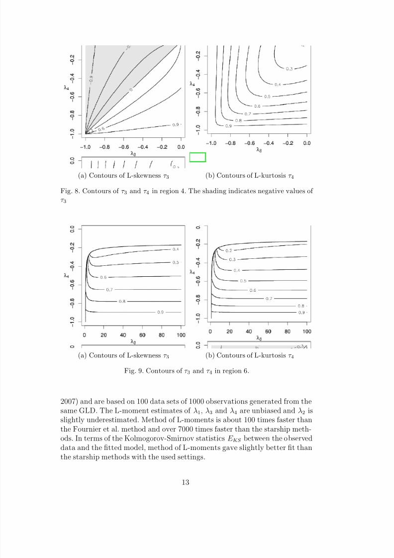
The contours of τ 3 and τ 4 in different GLD regions are shown in Figures 7, 8and 9. In region 3 the contours are rather complicated. From Figure 7(a) and7(c) it can be seen that there are three separate areas where τ 3 has negativevalues. It is also seen that besides the line λ3 = λ4, there are two curves whereτ 3 = 0. Naturally, the distributions defined by the curves are not symmetric;

they just have zero L-skewness.

5 Estimation by method of L-moments

In method of L-moments, we first calculate L-moments L1, L2, τ 3 and τ 4from the data. Then we numerically find parameters λ3 and λ4 that minimize

10



−10 −5 0 5 10 15

0 .

0

0 .

1

0 .

2

0 .

3

0 .

4

0 .

5

0 .

6

0 .

7

3(b)

3(a)

(a) from region 3

−10 −5 0 5 10 15

0 .

0

0 .

1

0 .

2

0 .

3

0 .

4

0 .

5

0 .

6

0 .

7

6

4

(b) from regions 4 and 6

Fig. 6. Pdfs of four GLDs with τ 3 = 0.4 and τ 4 = 0.25. The parameters of thedistributions are presented in Table 1.

some objective function that measures the distance between the L-skewnessand L-kurtosis of the data (τ 3, τ 4) and the L-skewness and L-kurtosis of theestimated model (τ 3(λ3, λ4), τ 4(λ3, λ4)). After that estimates λ1 and λ2 can besolved from equations (11) and (12). A natural objective function is the sumof squared distances

τ 3 − τ 3(λ3, λ4)

2+

τ 4 − τ 4(λ3, λ4)2

, (26)

which was used also by Asquith (2007).

We study the same simulation example that was studied by Fournier et al.(2007). They compare five estimators in situation where a sample of 1000observations is generated from GLD(0, 0.19, 0.14, 0.14), which is a symmet-ric distribution close to the standard normal distribution. We apply methodof L-moments to the same problem and present the results in a compara-ble form. Before carrying out the simulations, we analyze the example us-ing the results given in the preceding sections. Because λ3 = λ4 = 0.14,GLD(0, 0.19, 0.14, 0.14) is a symmetric distribution from region 3. The the-oretical L-moments L1 = 0, L2 ≈ 0.60407, τ 3 = 0 and τ 4 ≈ 0.12305 of GLD(0, 0.19, 0.14, 0.14) are obtained from equations (11)–(14). Because τ 3 = 0

we may apply equation (19) that gives the “correct” solution λ3 = λ4 = 0.14and another solution λ3 = λ4 ≈ 4.26316 also from region 3. By inspect-ing the contours in Figure 7 we find that there exist also two asymmetricGLDs from region 3 with τ 3 = 0 and τ 4 ≈ 0.12305. The numerical mini-mization of objective function (26) with suitable initial values gives solutions(λ3 ≈ 1.98, λ4 ≈ 22.59) and (λ3 ≈ 22.59, λ4 ≈ 1.98). Figure 10 shows thecontours of objective function (26) when τ 3 = 0 and τ 4 ≈ 0.12305. It can beclearly seen that the achieved numerical solution depends on the initial values

11



(a) Contours of L-skewness τ 3 (b) Contours of L-kurtosis τ 4

(c) Contours of L-skewness τ 3 (zoomed) (d) Contours of L-kurtosis τ 4 (zoomed)

Fig. 7. Contours of τ 3 and τ 4 in region 3. The shading indicates negative values of τ 3.

of λ3 and λ4.

In the simulation we choose a strategy where τ 4 computed from the dataand the two solutions of equation (19) are tried as initial values of λ3 and λ4.

The numerical optimization of the objective function (26) is carried out by theNelder-Mead method (Nelder and Mead, 1965) in R (R Development Core Team,2006) and the computer used for the simulation is comparable to the computerused by Fournier et al. (2007). The results from 10000 data sets of 1000 ob-servations generated from GLD(0, 0.19, 0.14, 0.14) are presented in Table 2.The first column of the table reports the L-moment estimates correspondingto the smaller initial solution which leads to the estimates corresponding tothe generating GLD. The last three columns are copied from (Fournier et al.,

12




Fig. 8. Contours of τ 3 and τ 4 in region 4. The shading indicates negative values of τ 3


Fig. 9. Contours of τ 3 and τ 4 in region 6.

2007) and are based on 100 data sets of 1000 observations generated from thesame GLD. The L-moment estimates of λ1, λ3 and λ4 are unbiased and λ2 isslightly underestimated. Method of L-moments is about 100 times faster thanthe Fournier et al. method and over 7000 times faster than the starship meth-ods. In terms of the Kolmogorov-Smirnov statistics E KS between the observeddata and the fitted model, method of L-moments gave slightly better fit thanthe starship methods with the used settings.

13



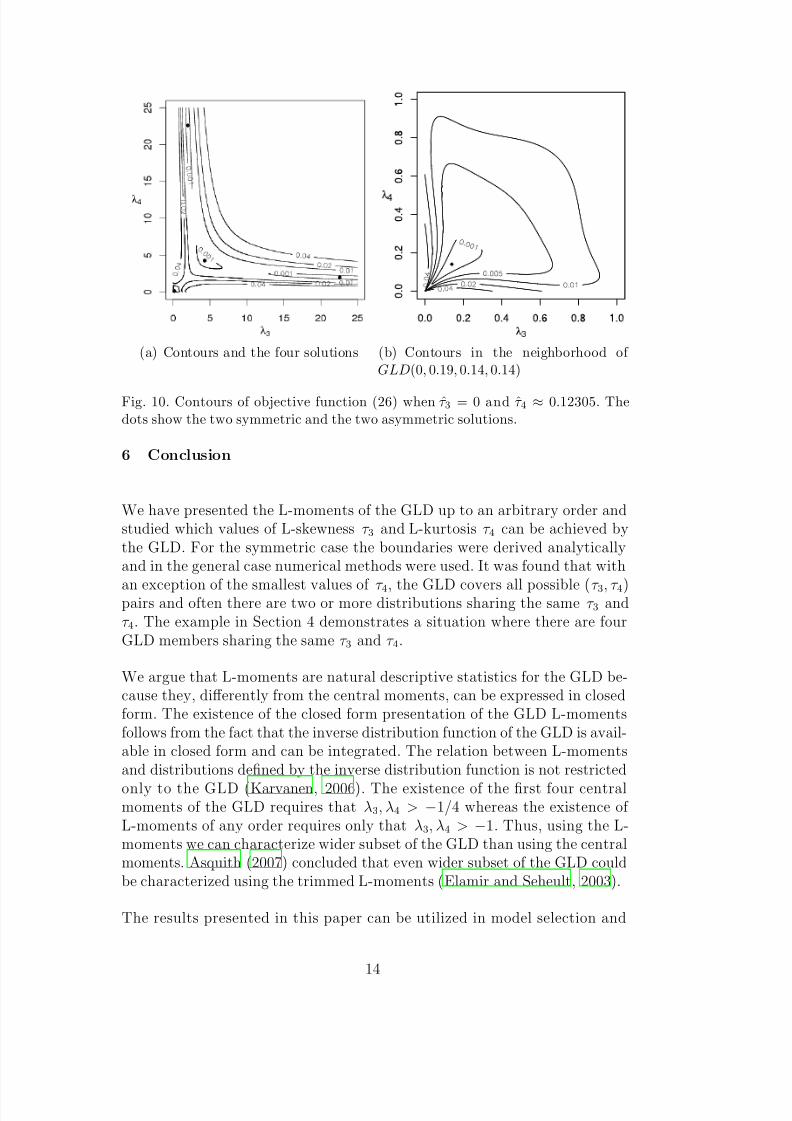
(a) Contours and the four solutions (b) Contours in the neighborhood of GLD(0, 0.19, 0.14, 0.14)

Fig. 10. Contours of objective function (26) when τ 3 = 0 and τ 4 ≈ 0.12305. Thedots show the two symmetric and the two asymmetric solutions.

6 Conclusion

We have presented the L-moments of the GLD up to an arbitrary order andstudied which values of L-skewness τ 3 and L-kurtosis τ 4 can be achieved bythe GLD. For the symmetric case the boundaries were derived analyticallyand in the general case numerical methods were used. It was found that with

an exception of the smallest values of τ 4, the GLD covers all possible (τ 3, τ 4)pairs and often there are two or more distributions sharing the same τ 3 andτ 4. The example in Section 4 demonstrates a situation where there are fourGLD members sharing the same τ 3 and τ 4.

We argue that L-moments are natural descriptive statistics for the GLD be-cause they, differently from the central moments, can be expressed in closedform. The existence of the closed form presentation of the GLD L-momentsfollows from the fact that the inverse distribution function of the GLD is avail-able in closed form and can be integrated. The relation between L-momentsand distributions defined by the inverse distribution function is not restricted

only to the GLD (Karvanen, 2006). The existence of the first four centralmoments of the GLD requires that λ3, λ4 > −1/4 whereas the existence of L-moments of any order requires only that λ3, λ4 > −1. Thus, using the L-moments we can characterize wider subset of the GLD than using the centralmoments. Asquith (2007) concluded that even wider subset of the GLD couldbe characterized using the trimmed L-moments (Elamir and Seheult, 2003).

The results presented in this paper can be utilized in model selection and

14



Table 2Comparison of estimation methods. The mean and the estimated standard errorof the L-moment estimators are computed from 1000 data sets generated fromGLD(0, 0.19, 0.14, 0.14). The results for the other methods are based 100 gener-ated data sets from the same GLD and are copied from (Fournier et al., 2007).Fournier et al. method is based on the percentile method and the minimization of the Kolmogorov-Smirnov distance in the (λ3, λ4) space. Starship KS and starshipAD methods correspond to the starship method (King and MacGillivray, 1999) us-ing the Kolmogorov-Smirnov or the Anderson-Darling distance, respectively.

Quantity L-moments Fournier et al. Starship KS Starship AD

λ1 Mean 0.00153 -0.00030 0.25010 0.00720

Std error 0.10287 0.05010 0.10000 0.07300

λ2 Mean 0.18795 0.19960 0.20020 0.19400

Std error 0.03625 0.05650 0.04760 0.03020

λ3 Mean 0.14012 0.15110 0.15530 0.14600

Std error 0.03602 0.05150 0.04630 0.03170

λ4 Mean 0.13981 0.15060 0.14750 0.14350

Std error 0.03573 0.05030 0.04510 0.02860

Time (s) Mean 0.02767 3.19010 206.99000 213.47000

Std error 0.00575 0.15020 40.42010 42.15210

E KS Mean 0.01597 0.01850 0.01680 0.01856

Std error 0.00319 0.00430 0.00270 0.00360

estimation. The characterization by L-moments gives an insight into which τ 3and τ 4 are available in each GLD region. For instance, there are symmetricGLD members available from both region 3 and 4, if τ 4 > 1/6. This kind of information is useful when making the decision whether the GLD is a potentialmodel for certain data. The results are also useful in the estimation of theGLD parameters. The parameters can be estimated directly by method of L-methods or the L-moment estimates can be used as starting values for otherestimation methods. In both cases, we can use the L-moment ratio boundariesto specify the potential GLD regions where we should search for the parameterestimates. The choice between alternative solutions can be based on the type

of the domain (bounded/unbounded) or some other additional criterion suchas the Kolmogorov-Smirnov statistic or L-moment ratios τ 5 and τ 6.

In the simulation example, method of L-moments compared favorably to morecomplicated estimation methods. Estimation by method of L-moments was thefastest in the comparison and the estimates were unbiased or nearly unbiased.The goodness of fit measured by the Kolmogorov-Smirnov statistic was thesame or better than with the alternative estimation methods. More simulations

15



are needed to find out how general these results are.

Acknowledgement

The authors thank William H. Asquith for useful comments.

References

Asquith, W. H., 2007. L-moments and TL-moments of the generalized lambdadistribution. Computational Statistics & Data Analysis 51, 4484–4496.

Bergevin, R. J., 1993. An analysis of the generalized lambda distribu-tion. Master’s thesis, Air Force Institute of Technology, available from

http://stinet.dtic.mil.Bigerelle, M., Najjar, D., Fournier, B., Rupin, N., Iost, A., 2005. Application

of lambda distributions and bootstrap analysis to the prediction of fatiguelifetime and confidence intervals. International Journal of Fatigue 28, 223–236.

Corrado, C. J., 2001. Option pricing based on the generalized lambda distri-bution. Journal of Future Markets 21, 213–236.

Elamir, E. A., Seheult, A. H., 2003. Trimmed L-moments. ComputationalStatistics & Data Analysis 43, 299–314.

Fournier, B., Rupin, N., Bigerellle, M., Najjar, D., Iost, A., Wilcox, R., 2007.

Estimating the parameters of a generalized lambda distributions. Compu-tational Statistics & Data Analysis 51, 2813–2835.Headrick, T. C., Mugdadib, A., 2006. On simulating multivariate non-normal

distributions from the generalized lambda distribution. ComputationalStatistics & Data Analysis 50, 3343–3353.

Hosking, J., 1990. L-moments: Analysis and estimation of distributions usinglinear combinations of order statistics. Journal of Royal Statistical SocietyB 52 (1), 105–124.

Hosking, J. R. M., 2006. On the characterization of distributions by theirL-moments. Journal of Statistical Planning and Inference 136 (1), 193–198.

Jones, M. C., 2004. On some expressions for variance, covariance, skewness

and L-moments. Journal of Statistical Planning and Inference 126, 97–106.Karian, Z. A., Dudewicz, E. J., 1999. Fitting the generalized lambda distribu-

tion to data: A method based on percentiles. Communications in Statistics:Simulation and Computation 28 (3), 793–819.

Karian, Z. A., Dudewicz, E. J., 2000. Fitting Statistical Distributions: TheGeneralized Lambda Distribution and Generalized Bootstrap Methods.Chapman & Hall/CRC Press, Boca Raton, Florida.

Karian, Z. A., Dudewicz, E. J., 2003. Comparison of GLD fitting methods:

16

http://stinet.dtic.mil/

http://stinet.dtic.mil/



Superiority of percentile fits to moments in L2 norm. Journal of IranianStatistical Society 2 (2), 171–187.

Karian, Z. A., Dudewicz, E. J., McDonald, P., 1996. The extended general-ized lambda distribution system for fitting distributions to data: History,completion of theory, tables, applications, the “final word” on moment fits.

Communications in Statistics: Simulation and Computation 25 (3), 611–642.Karvanen, J., 2003. Generation of correlated non-Gaussian random variables

from independent components. In: Proceedings of Fourth International Sym-posium on Independent Component Analysis and Blind Signal Separation,ICA2003. pp. 769–774.

Karvanen, J., 2006. Estimation of quantile mixtures via L-moments andtrimmed L-moments. Computational Statistics & Data Analysis 51 (2), 947–959.

Karvanen, J., Eriksson, J., Koivunen, V., 2002. Adaptive score functions formaximum likelihood ICA. Journal of VLSI Signal Processing 32, 83–92.

King, R., 2006. gld: Basic functions for the generalised (Tukey) lambda dis-

tribution. R package version 1.8.1.King, R., MacGillivray, H., 1999. A startship estimation method for the gener-

alized lambda distributions. Australian and New Zealand Journal of Statis-tics 41 (3), 353–374.

Lakhany, A., Mausser, H., 2000. Estimating parameters of generalized lambdadistribution. Algo Research Quarterly 3 (3), 47–58.

Lampasi, D. A., Di Nicola, F., Podesta, L., 2005. The generalized lambda dis-tribution for the expression of measurement uncertainty. In: Proceedings of IMTC–2005 IEEE Instrumentation and Measurement Technology Confer-ence. pp. 2118–2133.

Nelder, J. A., Mead, R., 1965. A simplex algorithm for function minimization.Computer Journal 7, 308–313.Ozturk, A., Dale, R., 1985. Least squares estimation of the parameters of the

generalized lambda distribution. Technometrics 27 (1), 81–84.Pal, S., 2005. Evaluation of non-normal process capability indices using gen-

eralized lambda distributions. Quality Engineering, 77–85.R Development Core Team, 2006. R: A Language and Environment for Statis-

tical Computing. R Foundation for Statistical Computing, Vienna, Austria.URL http://www.R-project.org

Ramberg, J. S., Schmeiser, B. W., 1974. An approximate method for generat-ing asymmetric random variables. Communications of the ACM 17, 78–82.

Schnute, J., Boers, N., Haigh, R., and others, 2006. PBSmapping: PBS Map-ping 2. R package version 2.09.

Su, S., 2007. Numerical maximum log likelihood estimation for generalizedlambda distributions. Computational Statistics & Data Analysis 51, 3983–3998.

17

http://www.r-project.org/

http://www.r-project.org/

characterizing gld via l-moments

Documents