December 1, 2011

Cheakamus Project Water Use Plan Cheakamus River Steelhead Adult Abundance, Fry

Emergence-timing, and Juvenile Habitat Use and Abundance Monitoring

Implementation Year 4 Reference: CMSMON-3

Cheakamus River Steelhead Juvenile and Adult Abundance Monitoring

Study Period: Fall 2010 – Spring 2011

Ecometric Research Josh Korman and Jody Schick

Instream Fisheries Research Caroline Melville and Don McCubbing

Cheakamus River Steelhead

Juvenile and Adult Abundance Monitoring

Fall 2010 – Spring 2011

Final Report

Prepared for BC Hydro

By

Josh Korman and Jody Schick

Ecometric Research

and

Caroline Melville and Don McCubbing

Instream Fisheries Research

December 1st, 2011

ii

Abstract

The Cheakamus River once supported a large and productive wild winter-run

steelhead population and a well-known steelhead fishery, and there is a desire among

stakeholders to improve freshwater rearing conditions to increase the abundance of this

population. A proportion of the Cheakamus River is diverted to the Squamish River for

power generation. In 2006, rules controlling the timing and extent of the diversion, which

affects the flow regime in the river downstream of Daisy Dam, were modified based on

recommendations from a Water Use Planning (WUP) process. The objectives of this

project are to determine if the number of juvenile and adult steelhead in the Cheakamus

River, and the freshwater survival rate of various juvenile stages, are affected by the

WUP flow regime, and more broadly, to determine how flow affects steelhead production

in this system. This will be accomplished through long-term monitoring of juvenile

abundance and adult returns.

Adult Returns Escapement of steelhead to the Cheakamus River has been conducted annually

since 1996 and is determined by combining data from snorkel swim counts and radio

telemetry. We conducted a total of 12 swim surveys and radio-tagged 46 fish steelhead in

the Cheakamus River in 2011. The tagging study provided an additional year of telemetry

data to estimate diver observer efficiency, survey life, and departure timing, which are

used in conjunction with count data in a model to estimate escapement. Escapement of

steelhead to the Cheakamus River in 2011 was 1071 fish (724 wild-origin, 347 hatchery-

origin) with a coefficient of variation (CV) of 0.15. The total rate of return of hatchery-

origin smolts released in 2007 and 2008 to mitigate effects of a sodium hydroxide spill

was 0.75% and 4.11%. We used information on relative differences in marine survival of

hatchery- and wild-origin steelhead from the Cheakamus River based on acoustic tagging

(Melnychuck et al. 2009) to estimate a marine survival rate for wild-origin smolts that

outmigrated in 2008 of 10.3%. Escapements in 2010 and 2011, even after excluding

hatchery-origin spawners, are the highest on record since 1996, largely due to high

marine survival of 2008 outmigrants. The high survival of 2008 smolts was very apparent

in the age structure of returning adults in 2010 and 2011, with 74% and 68% returning at

ocean ages 2 and 3 years, respectively. Returns of wild-origin fish in 2009 were the

iii

lowest on record, likely due to the impact of the sodium hydroxide spill on freshwater

juvenile survival. A preliminary stock-recruit relationship indicates that wild-origin

steelhead escapement in 2010 and 2011 was more than adequate to fully seed available

habitat. Although escapements in 2010 (1144) and 2011 (1071) were similar, egg

deposition in 2011 (3.2 million) was two-fold higher owing to the larger size of returning

spawners (dominantly ocean age 3 year fish) and higher proportion of females (0.6).

The creel survey and the logbook records from anglers who participated in the

tagging program in 2011 documented a total of 993 and 1412 hours of effort,

respectively. A total of 167 wild- and 46 hatchery-origin steelhead were landed. Catch

per effort in 2010 and 2011 was over 2.5-fold higher than in 2009 due to escapement

differences. The proportion of wild-origin steelhead in the catch was 0.43 in 2009, 0.70 in

2010, and 0.78 in 2011. This pattern reflects the declining proportion of hatchery fish in

the system over this period due to termination of hatchery stocking as well as the effects

of the sodium hydroxide spill and marine survival on wild returns. Hatchery-origin fish

returning in 2010 and 2011 were not required to mitigate the effects of reduced

recruitment caused by the spill because of higher than expected marine survival rate.

However these hatchery-origin fish were available to anglers and contributed to higher

catch per effort.

Escapement of steelhead to Brohm River in 2010 and 2011 was estimated based

on redd counts and was 70 spawners in both years, compared to estimates from a

resistivity counter of 65 and 54 spawners, respectively. Assuming both wild- and

hatchery-origin spawners can migrate into Brohm River (as confirmed by radio telemetry

in 2011), escapement estimates to Brohm derived from the product of the Cheakamus

escapement and the proportion of tagged fish immigrating into Brohm River (~ 6%) were

67 and 70 fish in 2010 and 2011, respectively. These estimates are very close to the redd-

based estimates, suggesting that redd counts provide a reliable and highly cost-effective

means to determine escapement in Brohm River.

Juvenile Abundance

Estimates of juvenile steelhead abundance in the Cheakamus and Brohm Rivers

were derived for fall 2008-2010 and spring 2009-2011 in the Cheakamus River, and fall

2009-2010 and spring 2009-2011 in Brohm River. These values can be used to track

iv

abundance and survival rates through time and to relate these patterns to spawning

escapement and changes in flow. Fall abundance estimates were based on electrofishing,

while spring estimates were based on both electrofishing and snorkeling. Mark-recapture

experiments in fall and spring were used to characterize detection probability (the

proportion of fish captured or detected). These values were used to expand counts at a

large number of index sites sampled by a single pass of effort. A hierarchical Bayesian

model (HBM) integrated these data to estimate abundance and uncertainty in abundance

estimates.

Index sampling sites covered 21% and 7% of the total useable shoreline length in

Brohm and Cheakamus Rivers in fall 2010, and 31% and 20% in spring 2011,

respectively. Median abundance estimates of age 0 steelhead in the Cheakamus River in

fall ranged from a high of 240,000 in fall 2008, to a low of 70,000 in 2010. Parr

abundances in the Cheakamus River in fall are likely biased low due to overestimation of

river-wide detection probability, and ranged from 5,000-26,000 for age 1 parr, and 2,000-

9,000 for age 2 parr. Age 0, 1 and 2 year abundance estimates in spring, all of which are

unbiased, ranged from 23,000-50,000, 3,000-18,000, and 2,000-4,000, respectively.

Estimates of age 0, 1, and 2 year abundance in Brohm River in fall ranged from 22,000-

24,000, 4,000-5,000, and 2,000-5,000, respectively. Estimates of age 0, 1, and 2 year

abundance in Brohm River in spring (excluding 2009 when electrofishing was not done

resulting in a negative bias in abundance) ranged from 4,600-5,300, 1,000-3,000, and

1,100-1,200. Abundance in Brohm for all age classes has been very stable through time.

Most abundance estimates for the Cheakamus and Brohm Rivers had coefficients of

variation of 0.2 or less, especially in recent years when sampling intensity has increased.

Survival rates for various life stages were computed from changes in abundance

estimates through time. In the Cheakamus River, egg – fall fry (age 0) survival rates

ranged from a high of 45% for the 2008 spawning cohort, to a low of 4% for the 2010

cohort. Survival from fall fry to the spring two winters later (when fish are age 1+)

ranged from 4-8% in the Cheakamus River, and 5-12% in Brohm River. Coefficient of

variation in these survival rates ranged from 0.22-0.30, which is relatively low

considering the challenges of estimating survival rates in moderate-sized river systems.

v

Estimates of steelhead smolt production derived from juvenile surveys in spring

2009 through 2011 were within 30% of estimates from the Rotary Screw Trap (RST).

This may indicate that our production estimates are relatively unbiased. However, the

comparison is a relatively insensitive test because of uncertainty in both juvenile survey-

and RST-based estimates, and uncertainty in assumptions required to convert abundance

of parr into smolt production. The comparison at least establishes that the juvenile and

RST-based estimates of juvenile production are in reasonably close agreement. However,

there were significant discrepancies in length distributions of fish captured and aged

during juvenile surveys compared to those from the RST program. In particular, it

appears that age 1 and 2 year steelhead parr captured during the juvenile surveys are too

small compared to the sizes of fish aged as 2 and 3 year smolts at the RST. We expected

the length frequency distributions for these age classes to differ by no more than 20-30

mm owing to the growth between the time juvenile surveys are conducted (early April)

and when most steelhead are captured at the RST (May). However, RST captured fish at

a given age (e.g. 2 years) tended to be 50-60 mm larger than fish of the same age

captured during juvenile surveys (age 1+ parr). As steelhead are unlikely to growth this

much in less than two months, we conclude that fish captured from juvenile surveys are

either over-aged, or fish from the RST program are under-aged. We suspect the latter is

more likely, but further work is required to evaluate the discrepancy. Regardless, stock-

recruit analysis and the comparison of juvenile survey- and RST-based abundance

estimates should be considered highly preliminary until this uncertainty is resolved.

The most significant finding from the juvenile analysis conducted to date is the

demonstration that reasonable precision in estimates of survival rates across various

freshwater juvenile life stages can be achieved. This will likely allow evaluation of the

effects of major changes in flow and other abiotic and biotic factors on juvenile survival

rates. Given reasonably accurate escapement estimates, we have also shown it is possible

to compute egg-fry and egg-parr survival rates, and all these rates can be compared over

time and to literature values in unregulated streams to evaluate potential effects of the

current and future flow regimes. As an example, the substantive decrease in egg-fall fry

survival in 2010 may be due to the much greater egg deposition in that year, resulting in

greater density dependent mortality. Alternatively, rapid stage reductions in summer of

vi

2010, aimed at increasing the catch of Chinook broodstock for Tenderfoot Ck. Hatchery,

may have increased the mortality rate on recently emerged steelhead using low angle

cobble bars that are highly vulnerable to dewatering. We should be able to resolve this

uncertainty based on data from 2011 where egg deposition was high and when these rapid

stage changes did not occur. If egg-fall fry survival rates for the 2011 cohort are similar

to those in 2008 and 2009, this would indicate that rapid stage changes can have a

substantive effect on production of steelhead. Our assessment should also be able to

resolve whether there is strong density dependence in survival rates for later stages (e.g.

for age 0 fish over winter) which could reduce the impacts of flow-related mortality on

freshwater production.

vii

Glossary of Terms and Abbreviations

Adipose Fin: A soft, fleshy fin found on the back of a fish behind the dorsal fin

and just forward of the caudal fin (tail). AIC: The Akaikie Information Criteria is a model selection criterion

based on parsimony where more complicated models, which may fit the data better, are penalized for the inclusion of additional parameters.

Anadromous: Fish that migrate from the sea to fresh water to spawn. Beta Distribution: In probability theory and statistics, the beta distribution is a family

of continuous probability distributions defined on the interval (0, 1).

Bias: How far the average statistic lies from the parameter it is

estimating. Binomial Distribution: A calculation that measures the likelihood of events taking place

where the probability is measured between 0 (the event will certainly not occur) and 1 (the event is absolutely certain).

CV: The Coefficient of Variation is a measure of the ability to

repeatedly obtain the same value for a single sample or method (i.e., duplicate or replicate analyses). It is computed by dividing the standard deviation by the mean.

Detection Probability: The fraction of a population in a specific area (e.g., a fish

sampling site) that is detected by a unit of effort (e.g., a single pass of electrofishing).

Escapement: That portion of a migrating fish population that is not harvested

and escapes to natural or artificial spawning areas. Fry: A stage of development in young salmon or trout. During this stage

the fry is usually less than one year old, has absorbed its yolk sac, is rearing in the stream, and is between the alevin and parr stage of development.

GIS: A Geographic Information System is used to store and display

spatially-reference data. HV: Horizontal visibility used in this study to measure the clarity of

water which effects detection probability.

viii

Lognormal Distribution: Statistical distribution for which the log of the random

variable is distributed normally. HBM: A Hierarchical Bayesian Model is most useful for data that is

composed of exchangeable groups, such as fish sampling sites, for which the possibility is required that the parameters that describe each group might or might not be the same.

IFA/IFO: Instream Flow Agreements and Instream Flow Orders are

operating rules used to regulate discharge in rivers. Length-Frequency: An arrangement of recorded lengths, which indicates the number

of times, each length or length interval occurs. Maiden Spawner: A steelhead adult returning to freshwater that has not spawned

before. Mark-Recapture: A method to estimate the size of a population. It usually involves

live-capturing salmon, marking or tagging them and releasing them back into the water at one location.

Maximum Likelihood: Maximum likelihood estimation (MLE) is a popular statistical

method used for fitting a statistical model to data. Orthophotograph: An orthophoto or orthophotograph is an aerial photograph

geometrically corrected ("orthorectified") such that the scale is uniform.

Parr: life stage of salmonid fishes, usually in first or second year, when

body is marked with parr marks Poisson Distribution: A theoretical distribution that is a good approximation to the

binomial distribution when the probability is small and the number of trials is large.

Posterior Distribution: The expected distribution of parameter values determined from a

Bayesian analysis that is based on prior information about the parameter as well as data being directly used in the estimation.

Precision: The measure of the ability to repeatedly obtain the same value for a

single sample or method (i.e., duplicate or replicate analyses). Precision can be quantified by calculated the coefficient of variation (CV).

ix

Prior Distribution: In Bayesian statistics, a prior probability distribution, often called simply the prior, expresses prior knowledge about the uncertainty in a parameter.

Q: An abbreviation for discharge.

Radio Telemetry: Automatic measurement and transmission of data from remote sources via radio to a receiving station for recording and analysis. In this context, it refers to the deployment of radio tags to provide information on the movement and distribution of adult steelhead while in freshwater.

Redd: A egg nest formed in the gravel by salmon and other fish.

Repeat Spawner: A steelhead adult returning to freshwater that has spawned before.

Smolt: A juvenile salmonid that is undergoing the physiological change to migrate from fresh to salt water

Stock-Recruitment: The relationship between the abundance of animals at one life

stage (e.g., spawners) relative their abundance at a later stage (e.g., smolts).

Survey Life: The length of time a surveyed object (e.g., a fish or redd) is visible

to an observer (e.g., how long a steelhead spends in the surveyed area).

Thalweg: The deepest part of a stream’s channel. TRIM: Electronic and hard copy maps of topography, streams, and other

features in BC at a 1:20,000 scale. WUP: The Water Use Planning process was used to define new flow

regimes and monitoring programs for dams operated by BC Hydro.

x

Table of Contents Abstract ............................................................................................................................... ii Glossary of Terms and Abbreviations .............................................................................. vii Acknowledgements ............................................................................................................ xi 1.0  General Introduction .................................................................................................. 1 

1.1 References .................................................................................................................. 5 2.0  Adult Returns ........................................................................................................... 11 

2.1 Introduction .............................................................................................................. 11 2.2  Methods.................................................................................................................... 14 

2.2.1  Swim Counts and Angler Surveys in the Cheakamus River......................... 14 2.2.2  Tagging and Radio Telemetry Surveys and Ageing ..................................... 15 2.2.3  Steelhead Escapement Model ....................................................................... 18 2.2.4  Stock-Recruit Analysis ................................................................................. 23 2.2.5  Hatchery Return Rates .................................................................................. 24 2.2.6  Redd and Resistivity Counter Data from Brohm River ................................ 24 

2.3  Results ...................................................................................................................... 27 2.3.1  Swim Counts and Creel Survey .................................................................... 27 2.3.2  Radio Telemetry and Age structure .............................................................. 27 2.3.3  Escapement Estimates ................................................................................... 31 2.3.4  Stock-Recruit Analysis ................................................................................. 32 2.3.5  Hatchery Return Rate and Estimation of Wild Marine Survival .................. 33 2.3.6  Redd and Resistivity Counter Data from Brohm River ................................ 35 

2.4  Discussion ................................................................................................................ 36 2.5  References ................................................................................................................ 38 

Process Model ........................................................................................................... 42 Observation Model.................................................................................................... 42 Parameters ................................................................................................................. 44 Data ........................................................................................................................... 44 Constants ................................................................................................................... 44 

Appendix A.2. Distribution of Radio Tagged Steelhead, 2001-2011. .............................. 69 3.0 Juvenile Steelhead Abundance .................................................................................. 77 

3.1 Introduction .............................................................................................................. 77 3.2 Methods.................................................................................................................... 78 

3.2.1  Sample Site Selection and Field Methods .................................................. 80 3.2.2  Analytical Methods ..................................................................................... 84 

3.3 Results and Discussion ............................................................................................ 86 3.3.1  Data Summary and Supporting Analyses ................................................... 86 3.3.3  Estimates of Juvenile Steelhead Abundance from the Hierarchical Bayesian Model 88 

3.4 Conclusions .............................................................................................................. 92 3.5 References ................................................................................................................ 94 

xi

Acknowledgements

This project was supported through a contract from BC Hydro to Ecometric

Research to provide data for the Cheakamus River Water Use Plan. Additional funding

for the steelhead radio telemetry program was provided by the Canadian National

Railway Company and the Habitat Conservation Trust Fund, respectively. Brent Mossop

and Ian Dodd provided technical and administrative support, respectively. Robert Ahrens,

David Bryan, Scott Decker, Caroline Melville, Brent Mossop, Mathew Rochetta, Jeff

Sneep, Mike Stamford, Pier van Dischoeck, LJ Wilson, Heath Zander assisted with the

fieldwork. Scott Decker and Don McCubbing provided estimates of age for juvenile and

adult steelhead, respectively. Heath Zander conducted the creel survey, and Caroline

Melville supervised the angler logbook, creel survey and telemetry programs. Brian

Klassen, Clint Goyette, Ken Meehan, Roman LeHockey, Don Moore, Stu Reynolds,

Daryl Ross, Tom Velisek, Nathan Webb, and Heath Zander captured adult steelhead and

recorded sampling effort for the radio telemetry and angler log book programs. Tami

Nicol and Darren Ham provided GIS data and expertise for habitat mapping. Andrew

Gelman and Robert Dorazio provided helpful suggestions on the structure of the juvenile

hierarchal Bayesian model. Stephen Vincent programmed the animation of radio tagged

steelhead distribution.

1

1.0 General Introduction

The Cheakamus River is a productive tributary of the Squamish River that

supports populations of steelhead, chinook, coho, pink, and chum salmon, as well as

resident populations of rainbow trout, bull trout, and other species. The Cheakamus River

has an unregulated mean annual discharge of 65 m3 · sec-1 (at the Brackendale gauge

location) and drains an area of 1032 km2 of the Coastal Mountain range in southwestern

B.C. (Fig. 1.1). It was impounded in 1957 by Daily Lake Dam and a proportion of the

water entering Daisy Lake Reservoir is diverted to the Squamish River for power

generation. The Cheakamus River, downstream of Daisy Lake Reservoir, extends 26 km

to its confluence with the Squamish River. Only the lower 17.5 kilometers of this river

are accessible to anadromous salmon and steelhead. As a result of the diversion, the

Cheakamus River downstream of the dam receives only a portion of its natural discharge,

and there is much interest in understanding how this altered flow regime effects fish

populations.

The Cheakamus River once supported a large and productive wild winter-run

steelhead population and a well-known steelhead fishery. Although adult steelhead

returns are much smaller today, it still attracts considerable angling effort and is likely

one of the more productive wild steelhead population in southern BC (Van Dischoeck

2000). Steelhead juveniles rear for two to four years in the Cheakamus River before

migrating to sea as smolts. Steelhead juveniles are potentially more sensitive than other

juvenile salmonids in the Cheakamus River to changes in flow because they have a

longer period of freshwater residency. All these factors contribute to a strong interest

among resource users and fisheries managers in determining whether changes in the flow

regime below Daisy Lake Dam are affecting steelhead in the Cheakamus River.

The timing and volume of diversion rates from the Cheakamus River, which

effects flow downstream of the dam, have varied considerably since impoundment. From

1958-1994, diversions were largely driven by power generation within the constraints of

the original water license. Historical operations did not always follow these constraints,

so the Department of Fisheries and Oceans issued an instream flow order (IFO) to BC

Hydro in 1997. This order was subsequently modified to become an instream flow

agreement (IFA). The IFA specified that the greater of 5 m3·sec-1 or 45% of the previous

2

seven days average inflow be released downstream (within a daily range of 37-52%). In

February 2006, the operating constraints were modified based on a recommended flow

regime from the Water Use Plan (WUP). The WUP flow regime was based on meeting

minimum flows at the dam and further downstream at Brackendale. Operating rules no

longer depend on releasing a fixed fraction of inflows to the reservoir. Under the WUP

regime, flows from the dam must now exceed 3 m3·sec-1 (November 1-March 31st) or 7

m3·sec-1 (April 1st-Octber 31st), and additional water must be released to maintain

minimum flows at Brackendale of 15 m3·sec-1 (November 1st-March 31st), 20 m3·sec-1

(April 1st-June 30th), or 38 m3·sec-1 (July 1st – August 15th or 31st). This history of

operations has led to a number of changes in the flow regime in the Cheakamus River. As

many of the operating rules focused on minimum flows, and the effect of operations on

flow in the Cheakamus River is greatest during winter when inflows are lowest, there has

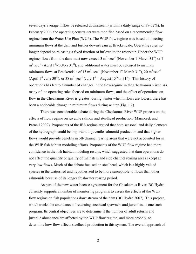
been a noticeable change in minimum flows during winter (Fig. 1.2).

There was considerable debate during the Cheakamus River WUP process on the

effects of flow regime on juvenile salmon and steelhead production (Marmorek and

Parnell 2002). Proponents of the IFA regime argued that both seasonal and daily elements

of the hydrograph could be important to juvenile salmonid production and that higher

flows would provide benefits in off-channel rearing areas that were not accounted for in

the WUP fish habitat modeling efforts. Proponents of the WUP flow regime had more

confidence in the fish habitat modeling results, which suggested that dam operations do

not affect the quantity or quality of mainstem and side channel rearing areas except at

very low flows. Much of the debate focused on steelhead, which is a highly valued

species in the watershed and hypothesized to be more susceptible to flows than other

salmonids because of its longer freshwater rearing period.

As part of the new water license agreement for the Cheakamus River, BC Hydro

currently supports a number of monitoring programs to assess the effects of the WUP

flow regime on fish populations downstream of the dam (BC Hydro 2007). This project,

which tracks the abundance of returning steelhead spawners and juveniles, is one such

program. Its central objectives are to determine if the number of adult returns and

juvenile abundance are affected by the WUP flow regime, and more broadly, to

determine how flow affects steelhead production in this system. The overall approach of

3

this project is relatively straightforward: 1) quantify escapement and juvenile abundance

in the fall and spring; 2) use these metrics to determine the survival rate between life

stages and define life stage-specific stock-recruitment relationships; and 3) over time,

compare abundance, survival rates and stock-recruitment relationships under different

flow regimes, and relate changes in these metrics to particular flow regimes or unique

flow events (Fig. 1.3).

Steelhead escapement to the Cheakamus River has been consistently assessed

since 1996 (Korman et al. 2007). The historical time series of escapement in part reflects

the rivers capacity to produce steelhead under pre IFA- and IFA-flow regimes. In the

future, this time series can be used to evaluate the WUP regime as well. The simplest way

to determine whether changes in flow have affected steelhead production is to compare

escapement over these time periods (e.g., Fig. 1.3a). However, as escapement is also

determined by parental abundance and marine survival, inferences from this comparison

may be weak unless flow effects are very large relative to these other factors. To address

this limitation, this project will estimate steelhead parr abundance in the spring as an

index of freshwater productivity during the period of freshwater residency (e.g., Fig.

1.3b). Each annual estimate of escapement and parr abundance will contribute a single

data point to estimate a freshwater stock-recruitment relationship between escapement

and parr abundance. The relationship controls for the effects of escapement on juvenile

production, and removes any effects associated with changes in marine survival (e.g.,

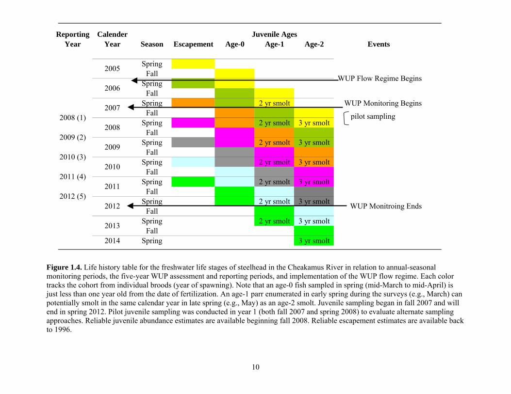
Fig. 1.3c). As data points accumulate (Fig. 1.4), it will be possible to relate outliers from

the escapement-to-parr stock-recruitment relationship, which indicate substantially higher

or lower juvenile steelhead production per unit escapement, to particular aspects of the

flow regime, such as the frequency and magnitude of high flow events during late fall, or

the duration of minimum flow periods during the winter. If the flow regime from Daisy

Lake Dam changes in the future, the escapement-to-parr stock-recruitment relationship

developed under the current WUP flow regime can be compared to a relationship

estimated under the new regime (e.g., Fig. 1.3c).

An escapement-to-parr stock-recruitment relationship is necessary for evaluating

population-level effects of flow, but provides little insight into what life stages are most

affected or which elements of the flow regime have the biggest effect on juvenile

4

steelhead survival. For example, higher flows during late fall could increase mortality of

recently emerged age 0 steelhead, but this mortality may not effect subsequent age 1

abundance and overall freshwater production because of compensatory survival

responses over the winter due to lower densities. To account for such dynamics, it is

necessary to quantify the stock-recruitment relationship for multiple juvenile life stages.

This project will therefore develop relationships between escapement and age-0 steelhead

in the fall, between age 0 fish in the fall and the following spring, and between age 0 and

age 1 fish in the spring (Fig. 1.3). The first relationship quantifies incubation success and

survival from emergence (summer) into the fall. The second quantifies age 0

overwintering survival. The third quantifies the annual survival rates for parr.

Uncertainties with regard to the stock structure of the Cheakamus River steelhead

population complicate the interpretation of the adult and juvenile abundance data. Brohm

River, a secondary tributary of the Cheakamus River (Fig. 1.1), is a potentially important

component of the steelhead production in the system. Between 10-40% of radio tagged

adult steelhead that entered the Cheakamus River survey area (upstream of the Cheekye

confluence) eventually migrated into Brohm River and spawned (Korman et al. 2005). To

determine the escapement in the Cheakamus River proper, escapement in Brohm River

therefore needs to be estimated so it can be subtracted from the aggregate estimate that is

currently obtained. In addition, an unknown proportion of juvenile steelhead that

originated in the Brohm River may migrate into the Cheakamus River and contribute to

the estimate of total abundance in the Cheakamus. Three working hypotheses can be used

to describe the range of possible dynamics between Brohm and Cheakamus stocks: 1)

Brohm and Cheakamus steelhead can be treated as a single stock. Returning adults have

no fidelity to the river they were spawned in, and juveniles fertilized in Brohm River can

migrate into and rear in the Cheakamus River; 2) Brohm and Cheakamus are completely

independent stocks. Adults always return to the river they were spawned in and juveniles

rear entirely in their natal systems; 3) An intermediate case where there is some site

fidelity and some straying among returning adults and rearing juveniles. This program

will attempt to evaluate the likelihood of these hypotheses through monitoring of

escapement and juvenile abundance in Brohm River.

5

This report summarizes and interprets data from the fourth year of the Cheakamus

River WUP steelhead monitoring project, covering the fall 2010 and spring 2011 surveys

(Fig. 1.4). See Korman 2008 and Korman et al. 2010 and 2011 for year 1, 2, and 3

results, respectively. The year 4 report is divided into two main chapters. Chapter two

summarizes the adult escapement methods and results, and includes a summary of creel

and telemetry information collected in 2009-2011 to determine the proportion of

hatchery- and wild-origin steelhead in the escapement. Chapter two also includes

information on adult escapement to Brohm River. Chapter three summarizes the methods

and results from the juvenile abundance program.

1.1 References

BC Hydro. 2007. Cheakamus River Water Use Plan Monitoring Terms of Reference.

Report prepared by BC Hydro, February 2007.

http://www.bchydro.com/etc/medialib/internet/documents/environment/pdf/enviro

nment_cheakamus_wup.Par.0001.File.environment_cheakamus_wup.pdf

Korman, J., Schick, J., Melville, C, and D. McCubbing. 2011. Cheakamus River

steelhead juvenile and adult abundance monitoring, Fall 2009 to Spring 2010

(Year 3). Report prepared for BC Hydro by Ecometric Research, August 2011.

http://www.bchydro.com/planning_regulatory/water_use_planning/lower_mainla

nd.html#Cheakamus

Korman, J., Schick, J., and A. Clark. 2010. Cheakamus River steelhead juvenile and adult

abundance monitoring, Fall 2008 to Spring 2009 (Year 2). Report prepared for

BC Hydro by Ecometric Research, February 2010.

http://www.bchydro.com/planning_regulatory/water_use_planning/lower_mainla

nd.html#Cheakamus

Korman, J. 2008. Cheakamus River steelhead adult abundance, and juvenile habitat use

and abundance monitoring 2007-2008 (Year 1). Report prepared for BC Hydro by

Ecometric Research, September 2008.

http://www.bchydro.com/planning_regulatory/water_use_planning/lower_mainla

nd.html#Cheakamus

6

Korman, J., Melville, C.C., and P.S. Higgins. 2007. Integrating multiple sources of data

on migratory timing and catchability to estimate escapement of steelhead trout

(Oncorhynchus mykiss). Canadian Journal of Fisheries and Aquatic Sciences

64:1101-1115.

Marmorek, D.R. and I. Parnell. 2002. Cheakamus River water use plan. Report of the

consultative committee. Report prepared on behalf of the Cheakamus River Water

Use Plan Consultative Committee by Essa Technologies Ltd.

Van Dischoeck, P. 2000. Squamish River system juvenile steelhead sampling program.

Report prepared for BC Ministry of Environment, Lands, and Parks by Aquatic

Resources Limited.

7

Figure 1.1. Map of the Cheakamus River study area showing the locations of the upstream limit of reach breaks used for habitat and juvenile surveys (open circles), distance (km) from the Squamish River confluence (gray points), migration barriers for anadromous fish in the Cheakamus and Brohm Rivers, and the Water Survey of Canada discharge gauge at Brackendale and rotary screw trap (RST).

#

#

#

#

#

#

#

BrackendaleGauge & RST

Reach 1

Cheekye River

Brohm River

Culliton Creek

Reach 2

Reach 3

Reach 4

Reach 5

MigrationBarrier

SquamishRiver

15.0

5.0

10.0

17.5

12.5

7.5

2.5

Migration Barrier& Reach 2

Reach 1

1 0 1 2 Kilometers

N

FigurCheaMarcpreviFebrugraphInstrehorizBrack

re 1.2. The aakamus Rivech was compious year (bauary, and Mah denote histeam Flow Azontal thick lkendale gaug

average minr, 1990-201

puted as the aased on averaarch for the toric operatiogreement (IFline shows thge.

imum flows1. The averaaverage of thage daily flocurrent yearons, and opeFA), and thehe 15 m3·sec

8

during wintage minimumhe minimumows), and ther (specified oerations undee current Wac-1 minimum

ter at the Bram flow betwe

m flow in Dece minimum fon x-axis). Ler the Instrea

ater Use Planm flow target

ackendale gaeen Decembcember fromflows in Janu

Labels at the am Flow Orn (WUP). Th

during wint

auge on the ber and m the uary, top of the der (IFO),

he dashed ter at the

9

Figure 1.3. Theoretical responses of escapement (a) and parr abundance (b) under two flow regimes, with 10 years of data collected under each regime, and the stock-recruit relationship between these life stages over the two periods (c). Solid and open circles represent data collected under flow regimes 1 and 2, respectively. Dashed horizontal lines in a) and b) represent the mean abundances over these periods. The solid line in c) represents the best-fit stock-recruitment curve under flow regime 1. Evidence for the effect of flow increases from a) to c) by reducing the confounding effects of marine survival (b) and the effects of both marine survival and density dependence (c).

0

200

400

600

2006 2008 2010 2012 2014 2016 2018 2020 2022 2024 2026 2028

Esc

apem

ent

a) Flow 1 Flow 2

0

20

40

60

80

2006 2008 2010 2012 2014 2016 2018 2020 2022 2024 2026 2028

Par

r A

bu

nd

ance

('0

00s)

b)

0

25

50

75

100

0 100 200 300 400 500 600 700Escapement

Par

r A

bu

nd

ance

('0

00s)c)

10

Figure 1.4. Life history table for the freshwater life stages of steelhead in the Cheakamus River in relation to annual-seasonal monitoring periods, the five-year WUP assessment and reporting periods, and implementation of the WUP flow regime. Each color tracks the cohort from individual broods (year of spawning). Note that an age-0 fish sampled in spring (mid-March to mid-April) is just less than one year old from the date of fertilization. An age-1 parr enumerated in early spring during the surveys (e.g., March) can potentially smolt in the same calendar year in late spring (e.g., May) as an age-2 smolt. Juvenile sampling began in fall 2007 and will end in spring 2012. Pilot juvenile sampling was conducted in year 1 (both fall 2007 and spring 2008) to evaluate alternate sampling approaches. Reliable juvenile abundance estimates are available beginning fall 2008. Reliable escapement estimates are available back to 1996.

Reporting CalenderYear Year Season Escapement Age-0 Age-1 Age-2 Events

SpringFall

SpringFall

Spring 2 yr smoltFall

Spring 2 yr smolt 3 yr smoltFall

Spring 2 yr smolt 3 yr smoltFall

Spring 2 yr smolt 3 yr smoltFall

Spring 2 yr smolt 3 yr smoltFall

Spring 2 yr smolt 3 yr smoltFall

Spring 2 yr smolt 3 yr smoltFall

2014 Spring 3 yr smolt

2008 (1)

2005

2006

2007

2008

2009

2010

2009 (2)

2010 (3)

2011 (4)

2013

2012

20112012 (5)

WUP Monitoring Begins

WUP Monitroing Ends

WUP Flow Regime Begins

Juvenile Ages

pilot sampling

11

2.0 Adult Returns

2.1 Introduction A program to estimate the annual number of adult steelhead returning to the

Cheakamus River (escapement) was initiated by BC Hydro in 1996. Escapement is an

important measure of population status and can be used to evaluate changes in freshwater

productivity affected by flow (Korman and Higgins 1997). However, as escapement may

also be effected by other factors such as marine survival rate, it will likely only be useful

for detecting very large flow-related effects (Bradford et al. 2005, Fig. 1.3a). To address

this issue, a significant portion of the Cheakamus WUP steelhead monitoring project

focuses on estimating juvenile abundance (section 4). Juvenile abundance will be more

sensitive to flow effects but can also be influenced by marine survival via its effect on

escapement (Fig. 1.3b). In particular, if marine survival rate is very low, escapement will

be low and could limit juvenile abundance (i.e., the system will not be ‘fully seeded’). By

developing relationships between escapement and the abundance of various juvenile life

stages, it is possible to evaluate whether this limitation is occurring and to correct for

such density dependent effects on juvenile abundance (Fig. 1.3c).

Escapement is estimated by fitting parameters of a run-timing model to count data

from repeat swim surveys conducted over the adult migration and spawning season

(Korman et al. 2007). Estimates of diver detection probability, survey life and departure

timing, determined from swim survey and radio telemetry data, are also incorporated in

the model. This section of the report provides an estimate of steelhead escapement to the

Cheakamus River in 2011. A synthesis of relevant physical data, other supporting

information required to generate the 2011 escapement estimate, and counts of resident

rainbow trout and char are also provided. Telemetry data collected in 2009-2011 resulted

in a modest change in escapement estimates over the entire time series because the

escapement model assumes that data on survey life and departure timing are

exchangeable among all years that surveys have been conducted. The version of the

model presented here stratifies telemetry-based data on detection probability into two

groups of years to avoid bias resulting from a reduction in detection probability in recent

12

years. We therefore present an updated time series of steelhead escapement estimates

from 1996 to the present.

We conducted a series of redd counts in Brohm River in 2011 to estimate

escapement. Brohm River is a tributary to the Cheekye River that enters the Cheakamus

River at the downstream boundary of the swim survey area (Fig. 1.1). Radio telemetry

has shown that between 6 to 41% (average 15%) of the tagged steelhead that enter the

lower survey area in the mainstem Cheakamus River eventually move into Brohm River

and spawn (Korman et al. 2011). Because of this behaviour, escapement estimates

currently generated for the Cheakamus River is an aggregate measure which includes the

escapement to the Cheakamus proper as well as some or all of the escapement to Brohm

River. By removing an estimate of the number of fish spawning in Brohm River from this

aggregate estimate, or a proportion of that estimate, it is possible to estimate escapement

to the Cheakamus River proper. Alternatively, the total escapement and the Brohm River

immigration rate can be used to estimate escapement in this tributary. Development of

independent time series of escapements for these two systems offers two advantages.

First, a time series of Brohm escapement estimates could potentially be used as an

‘experimental control’ to compare with trends in the Cheakamus River, since the

production of Brohm River smolts is not affected by flow regulation. As trends in

estuarine and marine survival rates for these two stocks are likely similar, any differences

in escapement trends would be attributed to differences in trends in freshwater

productivity between systems. However, Brohm River may only act as a pseudo-control,

since some juveniles fertilized there may migrate into the Cheakamus River and be

effected by flow releases from Daisy Lake Dam. Second, it is important to use

Cheakamus-specific escapement estimates in the development of escapement-juvenile

stock-recruitment relationships to assess flow effects.

A sodium hydroxid spill from a train derailment in the Cheakamus River canyon

in August 2005 killed approximately 90% of the juvenile steelhead population

(McCubbing et al. 2006). An experimental hatchery program was implemented shortly

after the spill to mitigate its effects on adult steelhead returns and speed the recovery rate

of the population. Approximately 20,000 steelhead smolts were released in the spring of

2007 and 2008. Assuming these smolts return to the Cheakamus River at the same ocean

13

ages as wild steelhead (2-3 yrs), escapement in 2009 through 2011 will be composed of

both wild- and hatchery-origin spawners. An accurate assessment of the effects of the

spill and the hatchery mitigation program on adult steelhead returns is necessary in order

to sensibly interpret the escapement time series with respect to flow regime effects (via

direct changes or escapement-juvenile stock-recruit analysis). Escapement estimates for

both wild- and hatchery-origin returns must be determined to do this (Table 2.1). With

respect to flow-related questions, we need to determine the extent to which the spill

reduced wild adult returns to decide which years should be removed from the WUP

analysis. The spill also provides a useful check on the sensitivity of wild escapement for

detecting changes in freshwater productivity. If a 90% mortality of juvenile fish cannot

be detected in the escapement trend, the trend is unlikely to be able to detect differences

caused by the switch from the IFA regime to the WUP regime. It is essential to remove

hatchery-origin adult returns from the WUP analysis of the escapement time series since

these fish were not produced in the Cheakamus River, and therefore were not affected by

flow regime. An estimate of the combined escapement of wild- and hatchery-origin fish

is needed to determine whether there were a sufficient number of returns to fully seed

available habitat to interpret the juvenile data. In this regard, it is essential to estimate

escapement for both stocks to develop an unbiased estimate of total escapement due to

potential differences in run timing and spatial distribution (effecting detection

probability) between stocks. Finally, marine survival rates can be accurately determined

for hatchery-origin fish since a known number of smolts are released. These survival

estimates, can be compared with those from other systems to guide future flow-related

decisions. For example, if marine survival rates for Cheakamus River steelhead are

similar to those in other systems, but escapement is much higher, this indicates that the

freshwater rearing environment in the Cheakamus is relatively productive which in turn

may temper our expectation about the extent to which productivity can be increased via

flow manipulation. It may also be possible to estimate marine survival rates for wild-

origin fish in the Cheakamus River using hatchery return rates and data comparing

hatchery and marine survival rates determined from acoustic tagging (Melnychuck et al.

2009).

14

Thus, to address the critical flow-related questions effected by the sodium

hydroxide spill, we modified the existing steelhead escapement model to estimate the

escapement of both wild- and hatchery-origin steelhead returns and report on results of

this new model. We use the estimated hatchery-origin escapement in 2009-2011 to

calculate the return rate for smolts released in 2007 and 2008. We examine the stock-

recruitment relationship between steelhead escapement and the adult returns produced in

the next generation using the historical time series. This provides information on the

escapement level required to attain the current adult carrying capacity for the system,

which in turn is used to evaluate the efficacy of the hatchery program with respect to its

objective of increasing the rate of recovery of the Cheakamus River steelhead population.

2.2 Methods

2.2.1 Swim Counts and Angler Surveys in the Cheakamus River Swim Counts

The Cheakamus River, downstream of Daisy Lake Reservoir, extends 26 km to its

confluence with the Squamish River. Only the lower 17.5 kilometers of this river are

accessible to anadromous salmon and steelhead (Fig. 1.1). The area surveyed for

returning steelhead was limited to the upper 14.5 km of the anadromous portion of the

river, and begins approximately 500 m below a natural barrier, extending to the

confluence with the Cheekye River. Higher turbidity and turbulence downstream of the

Cheekye confluence severely limit opportunities to conduct informative swim surveys. In

2011, twelve surveys were conducted between March 1st and May 5th. Survey methods

and timing were the same as previous assessments (Korman et al. 2010 and 2011,

Korman and McCubbing 2010). On each survey, a team of three divers floated the entire

survey area in four to six hours. The survey area is divided into 34 sections averaging 500

m in length. The number of steelhead (Oncorhynchus mykiss approximately >40 cm,

purple-silver hue, few black spots, fusiform shape), resident rainbow trout

(Oncorhynchus mykiss approximately 20-40 cm, darker coloration, black spots common

and large, more ‘blocky’ shape), and bull trout (Salvelinus confluentus) observed in each

section was recorded. Wild- and hatchery-origin steelhead captured by angling were

15

given pink and green spaghetti tags beginning in 2009, respectively (see section 2.2.2).

The number of tagged fish that were observed during swim surveys was also recorded.

Horizontal visibility (HV) was estimated by measuring the maximum distance from

which a diver could detect a dark object held underwater at 1 m depth. Horizontal

visibility was measured at 14.25 (section 4) and 7.65 (section 21) river kilometers (rkm)

upstream of the Squamish River confluence to index conditions upstream and

downstream of Culliton Creek, respectively (Fig. 1.1). Mean daily discharge (Q) over the

survey period was computed from the Water Survey of Canada (WSC) hourly discharge

record at the Brackendale gauge (WSC 08GA043). Hourly water temperatures were

recorded with an Onset Tidbit temperature logger placed at the North Vancouver Outdoor

School just downstream of the WSC Brackendale gauge.

Creel Survey A creel survey was conducted on the Cheakamus River from March 1st through

May 30th in 2009-2011 to quantify catch and effort for a sample of individual anglers.

The survey was not intended to quantify total angling effort or total catch. Each week a

maximum of eight hours was dedicated to the survey. All interviews were conducted in

the area between the Bailey Bridge (rkm 7.65) and Cheekye River confluence (rkm 3.65,

the downstream boundary of the survey area). We often arranged to meet anglers at the

end of the day to get a complete record of their day of fishing. During the interview, each

angler was asked to provide information on the number of hours fished, the number of

steelhead and other species that were captured, and whether the steelhead that were

captured had an adipose fin. Anglers participating in the tagging program (Section 2.2.2),

who have considerable fishing experience on the Cheakamus River, were given logbooks

to record similar statistics.

2.2.2 Tagging and Radio Telemetry Surveys and Ageing Steelhead were captured by skilled volunteer anglers fishing both within and

downstream of the survey area (Fig. 1.1). Methods were the same ones used in previous

telemetry efforts (Korman et al. 2007). Upon capture, a MCFT-3A radio tag (Lotek

Engineering Inc.) was placed in the stomach of each fish and a 6-inch fluorescent

spaghetti tag was attached through the dorsal muscle mass so that divers could visually

16

identify fish that were radio tagged to determine detection probability. Green and pink

colored tags were used to unambiguously distinguish wild- and hatchery-origin fish,

respectively. Fork length and gender were recorded during tagging and scale samples

were taken for ageing. Fish were held in a submersible holding tube for a minimum of

one-half hour prior to release to provide the fish a recovery period post handling and to

ensure that the radio tag was properly placed and that tag regurgitation had not occurred.

The movements of radio-tagged steelhead were determined using data from three

fixed telemetry stations and mobile tracking during the swim surveys. Mobile tracking

was conducted from a raft that followed 50-100 meters behind the divers on each survey

to identify the presence of tagged steelhead by river section using a Lotek SRX 400

version 4.01/W5 mobile receiver outfitted with a 3-element Yagi antenna (model F-3FB).

In addition, four mobile surveys of Brohm River, and two mobile surveys of the

Squamish River (from the Elaho and river mile 40 to the Cheakamus confluence were

completed in 2011. Fixed stations were located at the upstream and downstream

boundaries of the lower survey area (Fig. 1.1) and at the Brohm-Cheekye confluence.

Lotek SRX_400 receivers with CODE LOG W17 and W20 firmware were used at fixed

telemetry stations to record upstream and downstream movements.

The fixed station at the downstream end of the lower survey area was configured

so it could also record movement of fish up and down the Cheekye River. In 2010 and

2011, a fixed station was installed in Brohm River approximately approximately 75 m

upstream from the confluence with the Cheekye River. Telemetry stations consisted of a

12-volt deep cycle battery, a watertight enclosure, three 4-element Yagi antennas, double

insulated coaxial cable fitted with BNC connectors and an ASP-8 antenna-switching unit.

The antennas were pointed in the upstream and downstream directions of the Cheakamus

and Brohm Rivers. A third antenna was added to the lower station on the Cheakamus

River to detect upstream and downstream movement in the Cheekye River. The direction

of travel was determined based on the relative signal strength detected by each antenna

(Koski et al. 1993). Receivers at fixed telemetry stations were set up to continuously scan

all frequencies in use. When a steelhead outfitted with a digitally encoded tag moved

into detection range, the date, time, channel, code, signal strength and the antenna

number were recorded within the receiver’s memory. Fixed stations were installed well

17

before the deployment of the first radio tag (prior to February 25th) and were retrieved

well after the end of spawning and kelting period in mid-July.

Freshwater and ocean ages from the adult steelhead captured by anglers as part of

the tagging program in 2011 were estimated by scale reading. Approximately five scales

from each fish were collected from the preferred area above the lateral line and

immediately below the dorsal fin. Samples were placed in coin envelopes marked with

appropriate data for cross-reference. After a period of air-drying, scales pressed under

heat to provide images on soft plastic strips. These images were magnified using a

microfiche reader following the methods of Mackay et al. (1990). Age determination was

undertaken by the methods outlined in Ward et al (1989) and were the same as those used

in previous years. Two persons examined each scale sample set without knowledge of the

size or time and location of capture of the sampled fish. Samples were discarded when a

consensus between both persons could not be reached. At least one consistent scale

reader has been used since the inception of the program. We compare the 2011 age

estimates with those from previous years.

We analyzed a variety of models derived from radio telemetry to determine how

to structure the escapement model. The escapement estimation model includes

relationships that predict survey life, departure timing, and detection probability. We fit a

linear model predicting survey life as a function of data of entry. We fit a beta

distribution to the departure timing data to model the cumulative proportion of fish that

have left the survey area by specific dates. We used a logistic relationship to model how

detection probability varies with river conditions. For each of these models, the

unstratified simplest form was compared to more complex models that included

stratification by year, sex, and stock origin. We used the Akaikie Information Criteria

corrected for small sample size (AICc) to compare models (Burnham and Anderson

2002). Models with AICc values that are similar to the model with the lowest AICc score

were considered to have strong support (AICc = 0-2), while those with larger AICc

values were considered to have moderate (AICc = 4-7) or essentially no (AICc >10)

support.

18

2.2.3 Steelhead Escapement Model In order to determine the total escapement of returning spawners from periodic

swim counts, the proportion of fish observed by divers (detection probability) and the

fraction of the total run that is present on each survey is estimated (Korman et al. 2007).

Detection probability can be estimated based on the fraction of marked fish present in the

survey area that are observed, or by predicting it from river conditions. The fraction of

the run that is present on any survey can be estimated based on difference between the

cumulative proportion of the run that has arrived and the cumulative proportion that has

departed. An escapement estimation model quantifies these processes. The model

consists of three main elements. A process model predicts the number of fish present on

each day of the run and the departure schedule based on the total escapement and

relationships simulating arrival timing and survey life (the duration a fish resides in the

surveyed area given its date of entry). An observation model simulates the number of

marked and unmarked fish observed on each survey based on the number of tags known

to be in the survey area, predictions of the number of unmarked fish that are present, and

predictions of detection probability. A statistical model is then used to fit model

predictions to observations to compute the most likely estimates (MLEs) of model

parameters and to quantify uncertainty in these estimates.

Process and observation model parameters are estimated by maximizing the value

of a likelihood function that integrates data on the number of marked and unmarked fish

observed on each survey, the number of marks present in the survey area, survey life, and

departure timing. Data for the latter three elements were collected by marking fish with

an external spaghetti tag that could be identified by divers, and through radio telemetry.

This marking-telemetry program has been undertaken in eigth (2000, 2001, 2003-2005,

2009-2011) of 15 years that the swim surveys have been conducted (1996-2011,

excluding 1998). The model can be applied in years when marking-telemetry is not

conducted by assuming that data on the relationship between detection probability and

river conditions, survey life and date of entry, and data on departure schedules are

exchangeable among all years.

In order to estimate hatchery-origin steelhead escapement from 2009-2011, we

modified the Korman et al. (2007) model to predict escapement, and arrival and departure

19

timing for both wild- and hatchery-origin fish. The model predicts the numbers of both

stocks that are present on each survey, which in turn is used to determine the proportion

that are of wild origin by survey date. These proportions are statistically compared to

proportions based on the angler catch of wild- and hatchery-origin fish via an additional

term in the likelihood function. We assume that hatchery- and wild-origin stocks have

similar detection probabilities, survey lives (standardized by date of entry), and

vulnerabilities to being captured by anglers (see Appendix A of Korman et al. 2011).

More details of the model are described below.

Process Model

The proportion of the total escapement entering the survey area each day is

predicted separately for wild- and hatchery-origin stocks using a beta distribution (eqn.

2.1a, Tables 2.2 and 2.3). The beta distribution is parameterized so that β is calculated

based on estimates of the day when the peak arrival rate occurs (, or the mode of arrival

timing) and the precision of arrival timing (, eqn. 2.2), following the formulation in

Gelman et al. (2004). Note that small values of represent a low and constant rate of

arrival over the duration of the run, while larger values represent a shorter and more

concentrated arrival timing. A more flexible arrival model, which is not constrained by a

parametric function like the beta distribution, was included as an option in the new

escapement model. In this case, we estimate the proportion of the run arriving between

adjacent surveys (eqn. 1b). We refer to this latter model as the ‘deviate’ arrival-timing

model.

Survey life, that is, the number of days a fish spends in the survey area, is

predicted using a negative logistic function with respect to date of entry (i.e., fish that

arrive later have a shorter survey life, eqn. 2.3). We assume that wild- and hatchery-

origin stocks have the same survey life – date of entry relationship. Mean departure day

for fish arriving each day of the run is predicted based on the sum of the arrival day and

the survey life for fish arriving on that day (eqn. 2.4). The proportion of fish that arrive

on day i and depart on day j, which we term the arrival-departure matrix, is predicted

from a normal distribution (eqn. 2.5) and accounts for variation in survey life for a given

arrival day. Matrix values are standardized so that proportions across all departure days

for each arrival day sum to one, that is, all fish must exit the survey area by the assumed

20

last day of the run. The proportion of fish departing on each day is a function of arrival

timing and the arrival-departure matrix (eqn. 2.6). As the former values vary by stock

origin, departure timing also varies by origin. The number of fish present in the survey

area by stock on each day is the product of the total escapement and the difference in the

cumulative arrival and departure proportions (eqn. 2.7). Estimates of the cumulative

proportion of wild-origin steelhead that have arrived by model day are required for the

two-stock model. These proportions are determined based on the ratio of the cumulative

arrivals of wild-origin steelhead to the sum of cumulative arrivals across both stocks

(eqn. 2.8).

Observation and Statistical Models

Escapement, arrival timing, and survey life parameters, and those defining the

relationship between detection probability and the ratio of horizontal visibility to

discharge (HV/Q), are jointly estimated by maximum likelihood. Independent likelihood

terms are developed for different components of the model, and the log-likelihoods are

added together to give a total likelihood function.

The likelihoods of the number of marked (Lr) and unmarked (Lu) fish observed are

assumed to follow a Poisson distribution (eqn.’s 2.9 and 2.10). The terms Lr and Lu, as for

all that follow, represent the sum of log-transformed probabilities across observations.

Note that detection probability is a nuisance parameter that does not need to be directly

estimated. Instead, it is evaluated at its conditional maximum likelihood estimate for each

survey based on equation 2.11 (see Korman et al. 2007). That is, detection probability is

simply the ratio of the total number of fish observed (data) to the total number predicted

to be present. As predictions of the number present (Uo,i) are not independent across

surveys because they are linked through the model structure, the number of unmarked

fish contributes to the conditional estimate of detection probability. Detection probability

is assumed to be equivalent among hatchery- and wild-origin steelhead in the two-stock

model and is therefore based on the ratio of the total fish observed to the total present.

The ratio of horizontal visibility to discharge is a good predictor of detection

probability in the Cheakamus River (Korman et al. 2007). Physically-based detection

probability estimates are required to estimate the number of fish present on surveys

where there are no tagged fish in the survey area. In this analysis, we recognize that

21

physically-based detection probability predictions can also be used on surveys where tags

are present. Precision of a purely tag-based estimate of detection probability will be very

poor when the total number of tags present or the true detection probability, is very low.

In this situation, estimates of detection probability from the physically-based model,

which incorporates information on detection probability from multiple surveys within and

across years under similar environmental conditions, will make an important contribution

to the estimate of the numbers present.

A logistic model is used to predict detection probability based on the ratio of

horizontal visibility to discharge (eqn. 2.12). Two additional likelihoods for the observed

number of marked (Lpr) and unmarked (Lpu) fish can now be computed by replacing the

conditional detection probabilities (qi) in eqn.’s 2.9 and 2.10 with detection probabilities

by the physical model (pi, eqn.’s 2.13 and 2.14). Parameters of the p-HV/Q relationship

are jointly estimated with other model parameters using data from all surveys when tags

were present (eqn. 2.15). Two sets of p-HV/Q parameters are estimated for data collected

between 2000-2005 and 2009-2010. Escapement estimates prior to 2009 are based on the

former set, while estimates after that are based on the latter. Note that Lpr is the sum of

likelihoods across surveys in the year that escapement is being estimated for. Lp is the

sum of likelihoods across all surveys when tags were present over all years when

telemetry was conducted, excluding observations used in calculating Lpr to avoid double

counting.

The likelihood of the survey life data (Ls) is computed assuming normally

distributed error (eqn. 2.16). Note that the term sl in this likelihood function is a

nuisance parameter that is calculated at its conditional maximum likelihood estimate

based on eqn. 2.17 (Ludwig and Walters 1994). The likelihood of the observed number of

fish departing the lower survey area in a downstream direction by stock origin (Lo,d) is

computed assuming multinomial error (eqn. 2.18).

Estimates of the proportion of cumulative arrivals that are wild in origin by

survey date (eqn. 2.8) are compared to observed estimates of stock proportions

determined by the number of wild- and hatchery-origin steelhead landed by anglers. The

likelihood of the catch of wild-origin steelhead up to each survey date (Lf) is computed

assuming Poisson error, and depends on the total catch (wild and hatchery) up to each

22

survey date and the predicted cumulative proportion of wild fish (eqn. 2.19). This

approach assumes that wild- and hatchery-origin fish are equally vulnerable to anglers,

which is supported based on a re-analysis of data from the Chilliwack River designed in

part to test this assumption (Appendix A).

The total log-likelihood for all the data given a set of model parameters θ = o,

o,o, λm, λh, λs, ρh, ρs, was determined by summing all component log-likelihoods and

the penalty function (eqn. 2.20). In years when hatchery-origin steelhead are expected to

return (2009-2011), H, H,H are estimated by including LdH, and Lf in the total

likelihood. When estimating parameters for any particular year, note that the first four

terms of the total likelihood and Lf (eqn. 2.20) are evaluated based only on data collected

in that year, while the latter 4 terms depend on data collected over all years when

telemetry was conducted. The denominator of 2 in the total likelihood formula accounts

for the fact that observations of marked and unmarked fish are double-counted in the

overall likelihood because they are evaluated using both conditional MLE values (q from

eqn. 11) and physically-based predictions of detection probability (p from eqn. 2.12). The

first term of eqn. 2.20 does not contribute to the total likelihood in years where tagging

was not conducted, or for surveys where tags are not present in years when tagging is

conducted.

We used the year-independent model to estimate the historical time series of

escapement for the Cheakamus River steelhead population. This model estimates all

model parameters independently for each year. In years with only wild-origin steelhead

returning, eight parameters are separately estimated for each year. An additional 3

parameters are estimated in years when hatchery-origin fish are returning. To derive

estimates of the number of wild-origin fish from 1996-2010 and hatchery-origin fish in

2009 and 2010, a total of 118 parameters are estimated (1998 is excluded as no surveys

were conducted). A penalty term, used to constrain arrival timing on hatchery-origin fish

in the 2009 analysis (Korman and McCubbing 2010, Korman et al. 2010), was not

required for the current analysis. The current analysis stratifies p-HV/Q models by year

groups (< 2009, >=2009). This alters the trend in the expanded number present by survey,

resulting in more realistic run-timing for both hatchery- and wild-origin fish.

23

Escapement estimates were computed using the AD model builder software (Otter

Research 2004). Non-linear optimization was used to quickly find the maximum

likelihood estimates (MLEs) of parameter values. Uncertainty in MLEs was computed

using the delta method. Estimates of the expected (average) parameter values and 90%

credible intervals (10th and 90th percentiles) were calculated from posterior distributions

generated using Monte Carlo Markov Chain (MCMC) simulation. The posterior

distributions for each year were derived from a total of 50,000 simulations. Every 5th

value was retained to remove auto-correlation among adjacent estimates. Of the 10,000

remaining simulations, the first 1,000 records were discarded to remove initialization

(i.e., burn-in) effects. This sampling strategy was sufficient for the model to produce

stable posterior distributions (model convergence) for all parameters in all years.

2.2.4 Stock-Recruit Analysis The number of adult steelhead returning to the Cheakamus River will be

determined by freshwater and marine survival rates as well as the number of spawners

that produced the returns, often termed brood escapement or spawning stock. We

examined the relationship between spawning stock in each brood year and the resulting

adult returns using a stock-recruit analysis. To do this, the recruitment (Rt) paired with

the escapement (w t) in brood year t was calculated from,

6,66,5,55,4,44,3,33, ttWttWttWttWt PPPPR ,

where W is the wild-origin escapement in year t+a and P is the proportion of maiden fish

returning in year t at total age a. Age proportions were specific to years when ageing was

conducted, which occurred in years when telemetry was done (2000, 2003-2005, 2009-

2011). Age proportions in other years were held constant at the multi-year average (see

Table 2.9). As no escapement estimate was available for 1998, we averaged escapements

from 1997 and 1999 to calculate escapement for this year. This was necessary to compute

the spawning stocks for the 2001-2003 return years. Stock-recruit analyses of adult data

are traditionally only applied to semalparous species, or to immature stages of iteroparous

species. In the case of steelhead, which are iteroparous, the number of repeat spawners

must be removed from the number of recruits or they would be double-counted in the

stock-recruit analysis. We used the average repeat spawner rate based the complete

24

ageing dataset of 0.15 (see Table 2.9) to compute the number of maiden recruits (maiden

recruits = total recruits * (1-repeat spawner fraction)). We then plotted the number of

maiden adult recruits as a function of the spawning stock that produced it.

Estimates of spawning stock that determine subsequent recruitment can be

improved by accounting for inter annual variation in sex ratios and fecundity of

spawners. To evaluate these factors for Cheakamus steelhead, we computed egg

deposition in years when information on sex ratio and female fork length was available

from angling surveys. Annual egg deposition was computed as the product of total

escapement, the proportion of the escapement made up of females, and fecundity. The

latter was computed based on annual average female fork length from the Cheakamus

River and a fecundity-female fork length relationship for steelhead from the Keogh River

(Ward and Slaney 1993). The ratio of egg deposition to escapement was then computed

to determine how much variability in spawning stock across years is driven by

differences in the sex and size structure of returning adults.

2.2.5 Hatchery Return Rates Return rates for hatchery-origin steelhead smolts released into the Cheakamus

River in 2007 and 2008 were computed by dividing estimates of the hatchery-origin

escapement from these release groups by the number of smolts released. The former

estimates were determined by multiplying the hatchery-origin escapement in each year by

the proportion of fish originating from each release group, which was determined based

on the total age from a sample of fish captured by angling in each return year. Our

hatchery return rates apply to steelhead only and do not account for the fraction of

hatchery smolts that residualized. An estimate of the marine survival rate for wild fish

was determined by multiplying the hatchery return rate by the ratio of survival rates of

acoustically-tagged wild- and hatchery-origin steelhead. We use the terms return rate and

marine survival rate interchangeably in this analysis, even though freshwater mortality

during outmigration is included in both estimates.

2.2.6 Redd and Resistivity Counter Data from Brohm River We used a visual count of steelhead redds, or egg nests, to estimate escapement in

Brohm River. Redd surveys can be an effective, precise and unbiased indicator of

25

escapement if survey methods are consistent and if conditions are suitable (Dunham et al.

2001,Gallagher and Gallagher 2005). Brohm River is well suited to steelhead redd

counts for several reasons: its small size and clear water allow a single person to observe

the entire cross section of the riverbed with minimal lateral movement; there is high

contrast between disturbed and undisturbed gravel; and flow is relatively stable over the

migration and spawning period. All these attributes help ensure all redds constructed

between surveys are counted by the observer, a critical assumption in the assessment.

We assumed that all redds were created by steelhead, rather than resident rainbow trout.

This is likely the case, as otolith microchemistry indicated that over 90% of juvenile trout

sampled in Brohm River in spring 2009 had an anadromous maternal parent (Korman et

al. 2010).

In 2011, we conducted five surveys of the entire 2.4 km of Brohm River that is

accessible to steelhead at roughly two-week intervals between May 4th – June 23rd. The

two-week interval was the assumed longest time period where a redd constructed

immediately after one survey would still be visible during the next survey (Gallagher and

Gallagher 2005), which was confirmed in Brohm River in 2009 (Korman and Schick

2010). A single observer wearing polarized glasses walked downstream searching the

entire stream cross section for redds. The observer also carried a dive mask and snorkel to

check areas where surface turbulence or depth prevented a clear view of the riverbed.

Redds were identified by several characteristics: a) circular or dish-shaped depressions

often of brighter appearance than the surrounding area with a zone of deposition along

the downstream margin or ‘back-stop’; b) a deposit of unsorted bed material in the

depression; and c) over-steepened walls with substrate perched on the edge of the

depression (an indication of excavation by tail strokes rather than scour by flow). We

distinguished between ‘test digs’ and completed redds by the former’s more elongated

shape and lack of a ‘back-stop’ and deposition in the depression. In circumstances where

the disturbed area was much larger than typical redds, we looked for indications that

more than one redd was present based on the formation of multiple deposits and signs of

superimposition.

We recorded the position of each redd using a Garmin 60CX GPS and marked

them with a fluorescent pin. This allowed us to avoid counting the same redds on

26

different surveys, and therefore to determine the number of unique redds created over the

spawning period. The number of unique redds was converted to the number of female

spawners based on the assumption that each female digs on average 1.2 redds (Jacobs et

al. 2002). The number of females was then converted to the total number of spawners by

assuming a 1:1 sex ratio (see Table 3 of Korman and McCubbing 2005). Under these

assumptions, the total number of redds can be converted to the total escapement by

multiplying it by a redd-to-spawner conversion of 1.7 (i.e., 2 spawners/female / 1.2

redds/female = 1.7 spawners/redd).

A resistivity counter was installed in Brohm River approximately 75 m upstream

from the confluence with the Cheekye River in spring 2010 and 2011. The objectives of

this project were to derive an independent estimate of steelhead escapement (relative to

redd counts) and to better understand the relationship between migratory timing of adult

returns and flow in Brohm River1. In 2011, the counter operated between April 3rd and

June 9th. The number of upstream counts from the resistivity counter was converted to an

estimate of escapement in Brohm River. We first compared a histogram of peak signal

size (PSS) for each upstream passage event from the Brohm River counter with those

from a similar counters on the Chilcotin and Coldwater Rivers where video validation

was conducted (McCubbing data on file) to determine the minimum PSS value that

represented an upstream movement event for steelhead. The resulting total upstream

steelhead counts over time were expanded based on an assumed counter efficiency for

upstream movement events of 80%, a value determined from a similar counter on the

Chilcotin River based on video validation (McCubbing data on file). We assumed that the

corrected upstream count represents the total escapement. This approach assumes there

are no repeated upstream and downstream movements of individual fish over the counter

(‘cycling’ of fish). Data from the radio telemetry station at this location was used to

partially support this assumption.

We compare estimates of the number of spawners in Brohm River and entry

timing derived from redd counts with those determined by the resistivity counter. We

compared these values with a tag-based estimate of escapement for Brohm River,

1 The 2010 and 2011 resistivity counter was not funded or approved for funding by BC Hydro. This project was supported solely by Instream Fisheries Research and will be summarized in detail in a report prepared for Ministry of Environment.

27

calculated as the product of the proportion of steelhead radio tagged in the Cheakamus

River that moved into Brohm River and the total escapement estimate for the Cheakams

River.

2.3 Results

2.3.1 Swim Counts and Creel Survey Discharge in the Cheakamus River was generally low and steady for the majority

of the swim survey period in 2010, although, like in most other survey years, high flows

limited survey opportunities in May (Fig. 2.1). Water temperature during winter and

spring of 2011 increased from approximately 4 °C in February to almost 8 °C in May.

We conducted a total of 12 swim surveys in 2011 (Table 2.4). Counts of steelhead,

rainbow trout, and bull trout across surveys ranged from 52-157, 9-46, and 64-262 fish,

respectively. The peak count for steelhead was the highest on record since surveys began

in 1996.

Angling data provided useful information on steelhead origin. The creel survey

and the logbook records from anglers who participated in the tagging program

documented a total of 993, 1414, and 1458 hours of effort in 2009, 2010, and 2011,

respectively (Table 2.5). A total of 167 and 46 wild- and hatchery-origin steelhead were

landed in 2011, respectively. The catch of wild steelhead was very similar to that in 2010,

but the catch of hatchery steelehead was reduced by almost 50% in 2011, owing to the

fact that only ocean age 3 year returns from the 2008 smolt release were returning in

2011. Catch per effort in 2010 and 2011 was over 2.5-fold higher than in 2009. The

proportion of wild-origin steelhead averaged 0.43 in 2009, 0.70 in 2010, and 0.78 in

2011. In 2009, based on variation in proportions of wild- and hatchery-origin steelhead

captured in March, April, and May, hatchery-origin steelhead had a much later arrival

timing than wild-origin fish, but this was not evident in 2010, and barely evident in

2011(Fig. 2.2).

2.3.2 Radio Telemetry and Age structure A total of 126 resident rainbow trout and steelhead were captured by volunteer

anglers and were sampled for age in 2011. Forty-six of these fish that were classified as

28

steelhead in the field based on the criteria used for swim counts and were radio tagged

and marked with a spaghetti tag so detection probability by divers could be estimated

(Tables 2.6, 2.7). Tagging occurred downstream and within the survey area. In 2011,

hatchery-origin fish were about 100 mm larger than wild fish due to the fact that wild fish

consisted of ocean age 2 and 3 returns, while hatchery fish consisted only of ocean age 3

returns (as the last year of smolt release was 2008). Forty-four of the 46 radio tagged

steelhead could be aged. An additional 47 fish that were not radio tagged were aged, of

which 11 were resident and the remaining 38 were steelhead. All resident fish aged in

2010 were hatchery in origin (10) and 10 of 11 resident fish sampled in 2011 were

hatchery in origin.

The majority of wild-origin steelhead returning in 2011 were ocean age 3 years,

likely due to the high marine survival rates for outmigrating smolts in 2008 (Table 2.8).

The average proportion of ocean age 3 year wild-origin steelhead across all years where

ageing data is available was 0.32, compared to 0.63 in 2011. All hatchery-origin fish

returned at ocean age 3 years as the last year of smolt release was in 2008. A total of 11

hatchery-origin or ‘residuals’ were confirmed based on angling captures and ageing

between 2010 and 2011 (Table 2.9). Ten wild-origin resident rainbow trout were aged in

2011 and the dominant age was 5 years.

A summary of telemetry-based statistics relevant to estimation of steelhead

escapement across all years is provided in table 2.10. This includes information to

estimate detection probability (the cumulative number of tags available to be detected

across swims each year), survey life, and departure timing. A total of 209 tag-swim days

were accumulated in 2011, about 16% of the total available across the eight years of

available data. Fourteen survey life estimates were obtained in 2011 bringing the total to

71(of which 9 were hatchery-origin fish). To obtain a survey life estimate for an

individual fish, it must be tagged downstream of the survey area (i.e., below the Cheekye

confluence), move upstream into the survey area (based on detections at the Cheekye

fixed station and from mobile tracking), and eventually be detected leaving the survey

area in a downstream direction (based on detections at the Cheekye fixed station). In

2011, departure date could be unambiguously determined (based on a downstream

departure record at the Cheekye fixed station) for 30 steelhead, bringing the total

29

departure record to 184 observations (of which 29 were hatchery-origin fish). Three

steelhead that were radio tagged moved into and likely spawned in Brohm River, and one

of these fish was hatchery in origin (Table 2.11). Averaged across all years, 15% of the

271 steelhead that have been radio tagged moved into Brohm River. Estimates of the

proportion of fish spawning in Brohm River in 2010 (6%) and 2011 (7%) were about half

of the average across the eight years of available data.

A spatial representation of the location of tagged steelhead in the Cheakamus and

Cheekye/Brohm Rivers for all steelhead tagged since 2000 is presented in Appendix A.

In 2011, one hatchery-origin steelhead was tracked in the Tenderfoot Creek pond. In

addition, two wild-origin fish tagged in the Cheakamus River downstream of the

Cheekye confluence (but a few km upstream from the mouth of the Squamish-Cheekye

confluence), were tracked in the Squamish River at river mile 20 and 30, well above the

confluence with the Cheakamus, on May 19-20th. One of these fish (radio code 55) held

in the lowest pool in the survey area within the Cheakamus River until at least May 5th

before departing downstream and eventually moving up the Squamish. The other fish

(radio code 36) never moved into the survey area, so its residency in the Cheakamus

River prior to moving into the Squamish could not be determined. 2011 was the only year

where tracking in the Squamish River upstream of the Cheakamus confluence was done,

so we cannot comment on whether similar movement patterns occurred in other years.

Using all available data, survey life declined with date of entry and was longer for

males than for females (Fig. 2.3). There was strong support for a sex-stratified linear

model predicting survey life as a function of date of entry relative to an unstratified

model (Table 2.12). However, sex cannot be reliably determined during swim surveys, so

a sex-stratified survey life model cannot be used in the assessment. Relative to the

unstratified model, there was limited support for a year-stratified model (AIC~4).

Perhaps due to low sample size of hatchery-origin fish (n=9), the origin-stratified model

has similar predictive ability (similar AIC) to the unstratified model.

Departure timing in 2011 was similar to the timing in 2009-2011, which is later

than in earlier years (Fig. 2.4a). As in 2010, hatchery-origin steelhead in 2011 departed

the survey area about one-week later than wild-origin fish (Fig. 2.4b). Assuming survey

life of hatchery- and wild-origin steelhead is similar (as indicated by the AIC analysis in

30

Table 2.12), this implies that hatchery-origin fish arrive slightly later than wild-origin

fish, which is consistent with the creel and logbook data in 2009 and to a much lesser

extent in 2011 (Table 2.5). We fit beta distributions to the departure timing data using

nonlinear estimation to compare the effects of origin, sex, year, and combinations of

these factors on departure timing (Table 2.13). Of the five models that were examined,

the most complex model that allowed departure timing to vary by year and origin had the

strongest support and there was virtually no support for other models. The analysis

indicated that year explains more variability in departure timing than does origin or sex.

Unfortunately, escapement estimates are based on a model which stratifies departure

timing by origin only. It is not possible to account for variation in departure timing by

year in the modeling framework because departure timing is a derived parameter (see

eqn. 2.6 in Table 2.2).

A maximum of 26 radio and spaghetti tagged fish were present in the survey area

over 12 swim surveys in 2011 (Table 2.14) and over twenty tags were present on half of

these swims. The additional 209 tag-swim observations in 2011 (the sum of tags present

across all swims) brings the multi-year total to 1327 (Table 2.10). Across all 2011

surveys, detection probability averaged 0.21 (Table 2.14). Average detection probability

for wild-(0.19) and hatchery-origin (0.26) fish in 2011 were similar considering the

uncertainty in survey-specific estimates driven by relatively low sample sizes.

Aggregating data across all 3 years when hatchery-origin fish were present and tagged,

detection probabilities were very similar across these groups and there was no support for

an origin-stratified detection probability model (Table 2.15). Discharge (Q) and

horizontal visibility (HV) are important determinants of diver detection probability

(Korman et al. 2007). Combining data across all years when detection probability

estimates are available, the ratio of HV/Q explained 13% of the variation in detection

probability (p, Fig. 2.5). There is considerable scatter around the p-HV/Q relationship

because many values of p are highly uncertain when the number of tags present on that

survey is low. For values of HV/Q less than 0.25, detection probability was lower in

2009-2011 compared to earlier years. There was strong support for the model where p-

HV/Q parameters were uniquely estimated for periods 2000-2005 and 2009-2011 (model

2) compared to the unstratified model where only one group of parameters was estimated

31

(model 1, Table 2.16). This supports the estimation of two p-HV/Q relationships in the

escapement model for the 1996-2008 and >=2009 periods.

2.3.3 Escapement Estimates We fit the two-stock escapement model (Korman et al. 2011) to all years of data.

This was necessary since we assume that telemetry information is exchangeable among

years. Hence data collected in 2011 contributes to estimates in that year as well as

previous years. The expected value for wild- and hatchery-origin escapement in 2011 was

724 (CV=0.13) and 347 (CV=0.30), respectively. The expected value for the total

escapement was 1071 (CV=0.15). This estimate is similar to the 2010 estimate (1144)

and four-fold higher than the average escapement between 1996 and 2009. There was

some evidence in the creel data that the fraction of hatchery-origin fish was lower early in

the run (before April 1st) in 2011, so the model delayed arrival timing of hatchery-origin

fish (Fig. 2.6a) to predict the decline in the proportion of wild fish in the catch (Fig. 2.6f)

As a result of later run timing, the hatchery-origin escapement estimate in 2011 was more

uncertain than the wild-origin estimate. Later run timing results in the model predicting

that a larger proportion of the run is present later in the swim season when detection

probability is lower (late April, early May) and when swims are not possible (after early

May), leading to greater uncertainty. The model provided good fits to the expanded count

(Fig. 2.6b), departure timing data (Fig. 2.6c), survey life (Fig. 2.6e), angling-based stock

composition (Fig. 2.6f), and p-HV/Q data (Fig. 2.6h). In general, there was reasonable

agreement in the numbers present estimated by expanding counts based on the ratio of

tags detected to tags present (r/R points in Fig. 2.6b) and those based on the p-HV/Q

expansion (open points).

The historical escapement trend for the Cheakamus River can be segregated into 3

periods (Fig. 2.7). Returns were low (average 181) in years when the juveniles that

produced these returns reared in freshwater prior to the imposition of the Instream Flow

Agreement (IFA, escapement from 1996-2001), and the average was twice as high after

this but prior to the sodium hydroxide spill (362, escapement from 2002-2007). This

difference was statistically significant (p=0.008). Wild-origin escapement declined over

two consecutive years for returns produced from juveniles that were present in the river

during the spill (escapement in 2008, 2009). However, because of the exceptional

32

escapement in 2010 and 2011, the post-spill average of wild-origin steelhead (447) was

higher than the IFA/pre-spill average. A post-spill average that includes hatchery-origin

returns (668) is 1.8-fold greater than the IFA/pre-spill average.

2.3.4 Stock-Recruit Analysis We did not attempt to fit a stock-recruitment model to the data as the initial slope

of that relationship is poorly defined due to the absence of very low escapement values

(Fig. 2.8). There is no indication that recruitment declines with escapement over the

range of estimates that are available. The estimates suggest that escapements as low as

100-200 fish are sufficient to fully seed the river, and that the replacement level

(intersection of 1:1 and stock-recruit lines) is approximately 300 spawners. The 2006

positive outlier highlights the exceptional survival for this brood. This was the first brood

that spawned following the sodium hydroxide spill. Above average smolt production in

2008 (Melville and McCubbing 2010) indicate that the freshwater survival of this brood

was approximately 40% higher than normal, perhaps due to lack of intra- and inter-

specific competition and predation due to spill-related mortality. However, the

exceptional total survival rate for this brood was mostly driven by an increase in marine

survival inferred from the hatchery return rate for the 2008 release (see analysis below).

The 2004 negative outlier was likely caused by the sodium hydroxide spill which

severely limited freshwater production from this brood year.

There was substantive variation in the number of eggs deposited per spawner

across years due to differences in sex ratios and the average size of female spawners

(Table 2.17). Average fecundity varied from a low of 3,206 (2010) to a high of 4,885

(2011). The proportion of the escapement that were females varied from a low of 0.41

(2001) to a high of 0.61 (2011). Egg deposition varied from a low of 171,000 (2000) to a

high of 3,178,000 (2011). The ratio of egg deposition (in ‘000s) to total escapement

varied from a low of 1.4 (2010) to a high of 3.0 (2011) with an average of 2.1. Sex- and

size-structure information is only available for about ½ of years where escapement

estimates are available. In other years, an average multiplier of 2.1 would need to be

applied to translate spawning stock to egg deposition on the x-axis of the stock-recruit

curve. As most of the points on that curve do not have year-specific estimates, this results

in an equal shift along the x-axis for most points, resulting in a very similar stock-recruit

33

relationship. However, year-specific estimates of egg deposition will be useful in the

computation of egg-fry survival rates from the more recent juvenile data collected in

years when sex- and size-structure data for the escapement is available (see Section 3).

2.3.5 Hatchery Return Rate and Estimation of Wild Marine Survival Estimates of hatchery-origin steelhead escapement and age structure from 2009

through 2011 were used to evaluate the extent to which the hatchery program mitigated

spill impacts on adult returns (Table 2.18). Hatchery-origin steelhead escapement in

2009, 2010, and 2011 was 101, 436, and 347, respectively. These escapements were

assigned to the 2007 and 2008 release year based on the age-structure of hatchery-origin

fish in these years determined from scales (Table 2.8 and 2.18). The estimated total

return rate (i.e., the sum of ocean age 2 and 3 year returns for each smolt release) for the

2007 and 2008 smolt releases was 0.75% and 4.11%.

The return of wild steelhead from the 2006 brood year was much higher than

expected given the spawning stock that produced these fish (Fig. 2.8), especially when

one considers that few 3 yr smolts were expected to outmigrate in 2008 due to effects of

the sodium hydroxide spill. Differences in ocean age 2 yr return rates for the 2007 and

2008 release years indicate that marine survival for the 2008 release was 5.5-fold greater

than the marine survival for the 2007 release (Table 2.18). Estimated smolt production in

2008 from the RST program was 1.4-fold greater than other years when estimates were

available, and this estimate is likely biased low relative to other years due to the inability

to operate the traps over a larger proportion of the steelhead outmigration period

(Melville and McCubbing 2010). However, there is considerable overlap in confidence

intervals for the 2008 smolt production estimate relative to earlier years with lower

estimates. Assuming the 2008 increase is real and not due to sampling error, the higher

value in 2008 is surprising as it should have been approximately 30% lower than the

historical average due to the loss of 3 yr smolts resulting from the spill. In summary, high

adult returns in 2010 and 2011 were the result of greater than expected smolt production

and high marine survival, although the latter effect was very likely much more

significant.

We estimated marine survival rates for wild-origin steelhead smolts outmigrating

in 2008 based on hatchery return rates (Table 2.19) and an acoustic tagging study that

34

compared survival of wild- and hatchery-origin smolts (Melnychuck et al. 2009).

Average survival rate for tagged steelhead smolts released in the Cheakamus River to the

southern end of Howe sound in 2008 was 67% for wild-origin smolts and 27% from

hatchery-origin smolts. The wild-to-hatchery survival ratio based on these estimates was

2.5. The majority of survival differences occurred in freshwater, and likely reflects

mortality of fish not well adapted to escape predation in the wild. Estimated marine

survival rate for wild-origin smolts outmigrating in 2008 was computed as the product of

the wild-to-hatchery smolt survival ratio and the 2008 hatchery return rate, which was

10.3% (=2.5*4.1%). This estimate can be used to backcalculate 2008 wild smolt

production to determine if escapement and smolt production estimates are consistent

(Table 2.19). Total returns from smolts outmigrating in 2008, determined by ocean age 2

year returns in 2010 and ocean age 3 returns in 2011 was 1,121. Given a 10.3% wild

survival rate estimate, this implies that almost 11,000 smolts left the Cheakamus System,

1.6-fold higher than the estimate of 6,810 smolts (Melville and McCubbing 2009). This

discrepancy could be due to an underestimate of smolt production, or an overestimate of

escapement or marine survival rate. It is more likely that escapement is underestimated

because the late run component is difficult to assess due to poor counting conditions at

that time. We see no reason for a major bias in the marine survival rate, thus the most

likely cause for the discrepancy between estimated and back-calculated smolt production

is an underestimate of the former. In part this could be due to an inability to run the RSTs

during the latter part of the smolt run. It is also likely that there is substantive smolt

production below the RST (Melville and McCubbing 2009). Assuming the RST estimate

is unbiased, the comparison suggests that approximately 37% of the smolt production

from the Cheakamus River occurs downstream of the RST. In our comparison of

mainstem parr production based on juvenile surveys in the Cheakamus River, we

calculated 42.7 km of useable shoreline for the entire river, and 27.3 km upstream of the

RST. This indicates that 36% of the shoreline length is located below the RST, which is

very close to the discrepancy between estimated and back-calculated smolt production

estimates in 2008.

35

2.3.6 Redd and Resistivity Counter Data from Brohm River A total of 42 unique redds were enumerated over five surveys in 2011, which

translated to 70 spawners based on the 1.7 spawner-per-redd conversion (Table 2.20).

The 2011 estimate is exactly the same as the estimate from 2010. Spawn timing in

Brohm River, based on the temporal pattern in the cumulative number of redds (Fig. 2.9),

was approximately 3 weeks later in 2011 compared to 2010, likely due to the unusually

cool spring in 2011.

The total upstream arrivals for steelhead from the resistivity counter in 2011,

under an assumed 80% upstream counting efficiency, was 54 spawners (Table 2.20, Fig.

2.9). Down counts were not subtracted from the upstream counts to estimate escapement

because: 1) recycling of radio tagged fish around the counter was not observed (i.e. only

one upstream event followed by one downstream event was recorded for the tagged

fish); 2) entry dates were highly varied as were residence periods for tagged fish (range 9

to 26 days) indicating both up and down counts were likely from "new" fish rather than

from fish recycling over the counter over short time periods; and 3) all tagged fish

exhibited a single kelting event, that is, were detected on the Cheekye receiver shortly

after a downstream detection on the Bohm receiver (McCubbing and Melville 2010).

Timing of steelhead spawning in Brohm River in 2010 and 2011 based on redd counts

was virtually identical to spawn-timing inferred based on the net upstream arrivals of fish

past the resistivity counter. Brohm escapement based on redd counts in 2011was 25%

higher than the counter-based estimate, but estimates were very similar in 2010. The

discrepancy in 2011 could be due to an overestimate of the number of true redds, a

change in the number of redds/spawner, or an overestimation of the efficiency of the

counter. We do not have any data to distinguish among these hypotheses.

Assuming the 2011 counter-based escapement estimate is unbiased, the spawner-

per-redd conversion for Brohm River in 2011 was 1.26, compared to 1.55 based on 2010

data. A total of three of radio tagged steelhead migrated into Brohm River in 2011. All

three of these fish were males, and two were wild-origin. The estimated number of

spawners in Brohm River in 2011, based on the product of the total escapement to the

Cheakamus River (1071, which can include fish destined to spawn in Brohm River) and

36

this 7% Brohm migration rate (3 of 46 tags), was 67 fish, close to the estimate of 70 fish

based on redd counts (Table 2.20).

2.4 Discussion

The estimated steelhead escapement to the Cheakamus River in 2011 was 1071

fish (724 wild-origin, 347 hatchery-origin). The total return rate of hatchery-origin fish

from the 2008 release was 4.11% which was over 5-fold higher than the rate for the 2007

release (0.75%). These results indicate that the marine survival rate for 2008 outmigrants

was much higher than in 2007. The number of wild steelhead smolts in 2008 was 1.4-fold

greater than the historical average (Melville and McCubbing 2010), a surprising result

given the expected loss of age 3 yr smolts in 2008 due to the 2005 sodium hydroxide

spill. The unusually high wild adult return in 2010 and 2011 was therefore caused by both

higher than expected smolt production and marine survival for the 2008 outmigrating

cohort, although, as discussed above, the change in marine survival was very likely the

bigger factor. In contrast, returns of wild-origin fish in 2009 were the lowest on record,

likely due to the reduction in freshwater survival rates due to the spill coupled with lower

marine survival. Surviving hatchery-origin smolts released in 2007 combined with wild-

origin escapement produced a total return of 204 fish in 2009. The most recent stock-

recruit analysis indicates that this is a sufficient escapement to fully seed available habitat

under the assumption that hatchery-origin fish are as successful as wild-origin fish in

terms of reproducing in the wild. In 2010 and 2011, escapement of wild-origin fish alone

was well above the estimate of the full seeding requirement.

The angling data in 2011 indicated that hatchery-origin steelhead had a later

arrival timing, with few hatchery fish present prior to April 15th. This result contrasts

with the similar run timing of both stocks in 2010. In 2009, hatchery-origin fish arrived

considerably later than wild-origin fish (Korman and McCubbing 2010), and the

difference was greater than what was estimated in 2011. The 2009 difference is consistent

with the hypothesis that the return of hatchery fish in 2009 would be late given that the

brood stock from which they were produced were collected late in the run in 2006, and

that arrival-timing is a heritable trait (Groot and Margolis 1991). However, this pattern of

37

brood collection cannot explain the across-stock difference in run timing in 2011,

although the difference is much less than in 2009.

There was relatively good agreement between estimates of steelhead escapement

to Brohm River based on redd counts (70 in 2010 and 2011) estimates from the resistivity

counter (65 and 54), and those derived based on total Cheakamus escapement and

immigration rates of tagged fish into Brohm (67-70 fish). Assuming the counter-based

estimate is unbiased, the spawner-to-redd conversion for Brohm River ranges from 1.25-

1.5, slightly lower than the value derived from the literature of 1.7. The amount of

spawning gravel in Brohm River is quite limited, and it may be that the lower spawner-

to-redd conversion ratio in this system is caused by females having to dig more redds to

deposit their eggs because of limited gravel availability. Ideally, redd counts and

resistivity counter estimates would be obtained in additional years to determine how

stable the conversion ratio is through time. That said, the resistivity counter estimate is

subject to unknown error as is the redd count data, so it may be that differences reflect

these errors rather than variation in spawners per redd in Brohm. In 2010 and 2011, the

contribution of Brohm River spawners to the total escapement to the Cheakamus system

was low. However in years of low returns, this proportion may be higher and in these

circumstances, obtaining accurate estimates of Brohm River escapement increases in

importance.

38

2.5 References

Burnham, K.P., and D.R. Anderson. 2002. Model Selection and Multimodel Inference,

2nd edition. Springer-Verlag, NY.

Gelman, A., Carlin, J.B. Stern, H.S., and D.B. Rubin. 2004. Bayesian data analysis.

Chapman and Hall/CRC. 668 pp.

Groot, C., and L. Margolis. 1991. Pacific salmon life histories. UBC Press, Vancouver,

BC. 564 pp.

Korman, J., Schick, J., Melville, C, and D. McCubbing. 2011. Cheakamus River

steelhead juvenile and adult abundance monitoring, Fall 2009 to Spring 2010

(Year 4). Report prepared for BC Hydro by Ecometric Research, August 2011.

http://www.bchydro.com/planning_regulatory/water_use_planning/lower_mainla

nd.html#Cheakamus

Korman, J., Schick, J., Melville, C., and D. McCubbing. 2010. Cheakamus River

steelhead juvenile and adult abundance monitoring Fall 2009 – Spring 2010.

Report prepared for BC Hydro by Ecometric Research, February 2010.

http://www.bchydro.com/planning_regulatory/water_use_planning/lower_mainla

nd.html#Cheakamus

Korman, J., Schick, J., and A. Clarke. 2010. Cheakamus River steelhead juvenile and

adult abundance monitoring Fall 2008 – Spring 2009. Report prepared for BC

Hydro by Ecometric Research, February 2010.

http://www.bchydro.com/planning_regulatory/water_use_planning/lower_mainla

nd.html#Cheakamus

Korman, J., and D. McCubbing. 2010. Evaluation of the effects of the 2005 sodium

hydroxide spill on steelhead escapement to the Cheakamus River in 2009 and the

efficacy of the first year of hatchery supplementation. Report prepared by

Ecometric Research and Instream Fisheries Research for the Canadian National

Railway Company.

Korman, J., C.C. Melville, and P.S. Higgins. 2007. Integrating multiple sources of data

on migratory timing and catchability to estimate escapement for steelhead trout

(Oncorhynchus mykiss). Can. J. Fish. Aquat. Sci. 64: 1101-1115.

39

Korman, J., and D.J. McCubbing. 2007. 2007 steelhead escapement to the Cheakamus

River. Report prepared for BC Hydro by Ecometric Research.

Korman, J. P.S. Higgins, and C.C. Melville. 2005. Incorporating the effects of migratory

behaviour and river conditions into estimates of steelhead escapement. Report

prepared for BC Hydro and the BC Habitat Conservation and Trust Fund by

Ecometric Research.

Koski, W.R, Link, M.R and K.K. English. 1996. Distribution, timing, fate and numbers

of chinook salmon returning to the Nass River watershed in 1992 Can. Tech. Rep.

Fish. Aquat. Sci.. 1996, 152 pp

Labelle, M. 2006. Evaluation of alternate recovery strategies for the Cheakamus River.

Interim report submitted to BC Ministry of Environment, April 25, 2006.

Ludwig, D., and C. Walters, 1994. Calculation of Bayes posterior probability

distributions for key population parameters. Can. J. Fish. Squat. Sci. 51: 713-722.

Mackay, W.C., G.R. Ash and H.J. Norris. 1990. Fish ageing methods for Alberta. R.L &

L. Environmental Services Ltd. in association with Alberta Fish and Wildlife

Division and University of Alberta, Edmonton. 133p.

Melville, C., and D. McCubbing. 2009. Cheakamus River- Juvenile Salmonid

Outmigration Enumeration Assessment Spring 2008. Report prepared for BC

Hydro by Instream Fisheries Research.

McCubbing, D.J.F and C.C Melville. 2010. Utility of a flat pad resistivity fish counter in

enumerating steelhead spawners on the Brohm River in 2010. Memo to MoE

from InStream Fisheries Resarch Inc, in prep.

McCubbing, D.J.F 2009. Adult Steelhead trout (Oncorhynchus mykiss) and salmonid

smolt migration at the Keogh River ,B.C., during winter 2008 and Spring 2009.

MoE Fisheries Project Report No. RD130. 2010 32p

McCubbing, D.J.F., Melville, C.C., Wilson, G., and M. Foy. 2006. Assessment of the CN

Rail caustic soda spill August 5th, 2005 on the fish populations of the Cheakamus

River. Report prepared by Instream Fisheries Research Inc.

Melnychuk, M.C., S. Hausch, D.F.J. McCubbing, and D. Welch. 2009. Acoustic tracking

of hatchery-reared and wild Cheakamus River steelhead smolts to address

40

residualization and early ocean survival. Report prepared for Canadian National

Railway Company, Monitor 2, project F. Available online at www.certc.ca.

Nelson, T.C., Rosenau, M.L., and N.T. Johnston. 2005. Behaviour and survival of wild

and hatchery-origin winter steelhead spawners caught and released in a

recreational fishery. North American Journal of Fisheries Management. 25: 931-

943.

Otter Research Ltd. 2004. An introduction to AD Model Builder version 7.1.1. for use in

nonlinear modeling and statistics. 194 pp. Report available from otter-rsch.com.

Ward, B.R., and P.A. Slaney. 1993. Egg-to-smolt survival and fry-to-smolt density

dependence of Keogh River steelhead trout. In Production of juvenile Atlantic

salmon, Salmo salar, in natural waters, Gibon, R.J. and R.E. Cutting [Eds.]. Can.

Spec. Publ. Fish. Aquat. Sci 118.

Ward, B. R., Slaney.P.A., Facchin, A.R, and Land. R.W. 1989. Size-based survival in

steelhead trout: back calculated lengths from adults’ scales compared to migrating

smolts at the Keogh River, B.C. Can. J. Fish. Aquat. Sci. 46:1853-1858.

41

Table 2.1. Indicators estimated by the current Cheakamus River steelhead escapement program in relation to key questions related to assessing the effects of flow regime and the effects of the CN sodium hydroxide spill.

Indicator Flow Regime Assessment Spill Assessment Wild Escapement

1. What years of WUP escapement time series are potentially effected by spill?

2. Can escapement detect major

changes in freshwater survival rate?

Did spill effect wild returns as predicted?

Hatchery Escapement

What fraction of adult returns was derived from fish not produced in Cheakamus River, and therefore not influenced by flow regime?

Was hatchery program effective at mitigating impacts of spill on adult returns?

Total Escapement

1. Was total escapement sufficient to fully seed river and therefore not limit juvenile abundance or future adult returns (assuming equal productivity among wild and hatchery components)?

2. Can we reliably estimate total escapement in years with wild

and hatchery returns if there are differences in return timing and distribution among stocks?

Hatchery Return Rate

How does marine survival for Cheakamus Steelhead compare to other systems (Keogh)? What is the marine survival rate for wild-origin steelhead from the Cheakamus River?

Was hatchery program effective?

42

Table 2.2. Equations used in the model to estimate steelhead escapement from swim survey, radio telemetry, and angler catch data. See Table 2.3 for definition of model variables. Eqn. # Description Equation

ProcessModel2.1 Arrival Timing a) beta model: 11

, )1( ooiiioPA

b) deviate model: iioPA ,

2.2 Transformation of arrival timing parameters

oo

oo

T

21

2.3 Survey life – date of entry )1(

ss

s

i

iSL

h

mt

2.4 Departure day ii SLid

2.5 Proportion arriving on day ‘i’ that depart on day ‘j’

),,(, sliji djNormalPAD

2.6 Departure timing ji

iiojo PADPAPD ,,, *

2.7 Number present by model day

i i

oooio PDPAU1 1

,

2.8 Proportion of wild-origin fish that have arrived by model day

i i

HHWW

i

WW

iw

PAEPAE

PAE

P

1 1

1,

ObservationModel2.9 Likelihood for marked fish

observed (Lr) )(~ iii RqPoissonr

2.10 Likelihood for unmarked fish observed (Lu)

))((~ ,, iiHiWii RUUqPoissonu

2.11 Conditional MLE of detection probability

iHiW

iii UU

urq

,,

2.12 Detection probability based on physical conditions

s

s

s

i

ih

i

i

i

QHV

QHV

p

2.13 Likelihood for marked fish observed in current year based on p from eqn. 2.12 (Lpr)

)(~ iii RpPoissonr

43

Table 2.2. Con’t. Eqn. # Description Equation

2.14 Likelihood for unmarked fish

observed in current year based on p from eqn. 2.12 (Lpu)

))((~ ,, iiHiWii RUUpPoissonu

2.15 Likelihood for marked fish observed from other years based on p from eqn. 2.12 (Lp)

)(~ iii RpPoissonr

2.16 Likelihood for survey life (Lsl) ),,(~ slii SLiNormalslobs

2.17 Conditional MLE for the standard deviation in survey life – date of entry relationship 1

)( 2

n

SLslobss ii

sl

2.18 Likelihood for departure timing (LdW and LdH)

),(~ ,,, ioi

ioio PDNexitMultinomNexit

2.19 Likelihood of stock composition given catch data (Lf)

))((~ ,,,,, iHiWiWiW CCPPoissonC

2.20 Total Likelihood (LT)

HpenLLLLL

LLLLdataL

fdHdWsp

puuprrT

22

)|(

44

Table 2.3. Definition of variables used in the steelhead escapement model.

Symbol Definition State Variables PAo,i Proportion of stock ‘o’ arriving on day ‘i’ PADi,j Proportion arriving on day ‘i’ that depart on day ‘j’ PDo,j Proportion departing for stock ‘o’ on day ‘j’ Uo,i Number present for stock ‘o’ on day ‘i’ Pw,i Cumulative proportion of wild-origin fish that have arrived by day ‘i’ di Mean departure day for fish arriving on day i pi Predicted detection probability on day ‘i’ based on physical conditions

Parameters Escapement for stock ‘o’ o Model day where the maximum arrival rate of stock ‘o’ occurs o Precision of arrival timing for stock ‘o’ o Transformed parameter for arrival timing model for stock ‘o’ i The proportion of the run that has arrived between survey ‘i-1’ and ‘i’ λm Maximum mean survey life (days) λh Model day where survey life is ½ the maximum λs Slope of the survey life – date of entry relationship h HV/Q ratio at which detection probability is 0.5 s Slope of the qP-HV/Q relationship Conditional Parameter (calculated) qi Detection probability on day ‘i’ sl Standard deviation (error) in survey life – date of entry relationship

DataRi Number of tags in survey area on day ‘i’ ri Number of tags observed on day ‘i’ ui Number of untagged fish observed on day ‘i’ HVi/Qi Ratio of horizontal visibility to discharge on day ‘i’ slobsi Observed survey life on day ‘i’ n # of observations of survey life Nexito,i # of fish of origin ‘o’ departing on day ‘i’ Co,i Cumulative landed catch of fish of origin ‘o’ by day ‘i’

Constantsi, j Indices for model day T Maximum model day (T=181) o Stock origin (wild: o=W, hatchery: o=H) i Proportional model day (i/T ranging from 0-1)

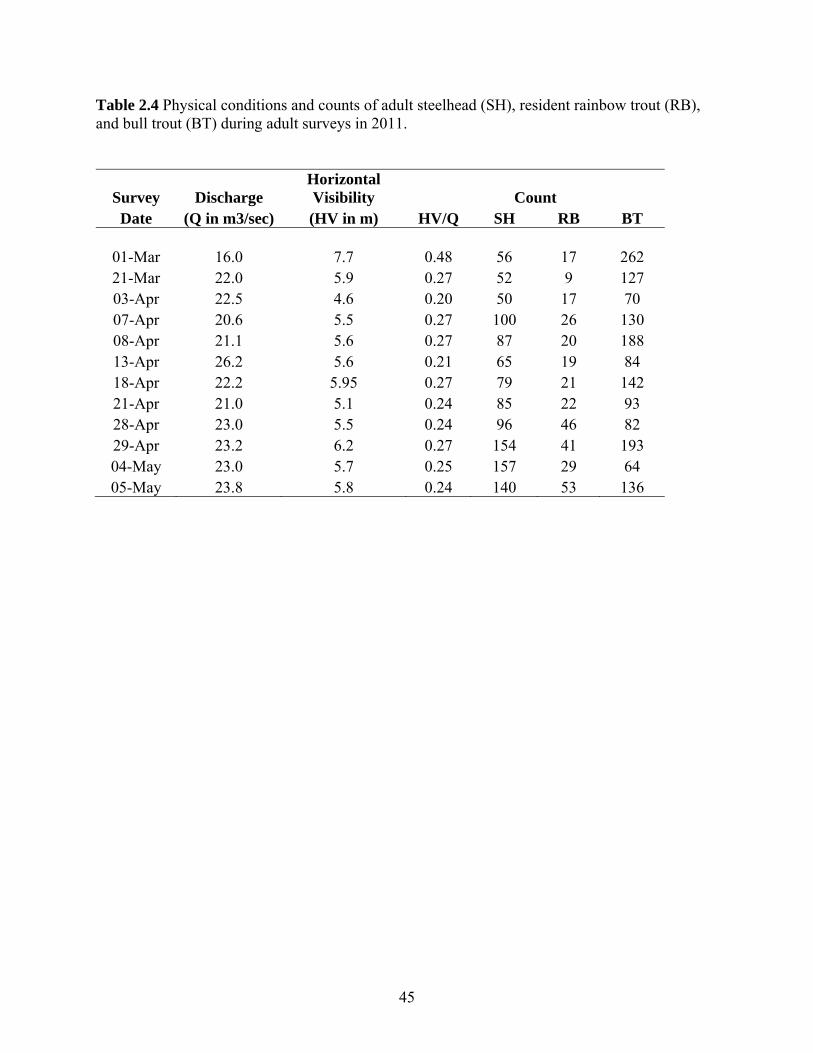
45

Table 2.4 Physical conditions and counts of adult steelhead (SH), resident rainbow trout (RB), and bull trout (BT) during adult surveys in 2011.

Survey Discharge Horizontal Visibility Count

Date (Q in m3/sec) (HV in m) HV/Q SH RB BT

01-Mar 16.0 7.7 0.48 56 17 262 21-Mar 22.0 5.9 0.27 52 9 127 03-Apr 22.5 4.6 0.20 50 17 70 07-Apr 20.6 5.5 0.27 100 26 130 08-Apr 21.1 5.6 0.27 87 20 188 13-Apr 26.2 5.6 0.21 65 19 84 18-Apr 22.2 5.95 0.27 79 21 142 21-Apr 21.0 5.1 0.24 85 22 93 28-Apr 23.0 5.5 0.24 96 46 82 29-Apr 23.2 6.2 0.27 154 41 193 04-May 23.0 5.7 0.25 157 29 64 05-May 23.8 5.8 0.24 140 53 136

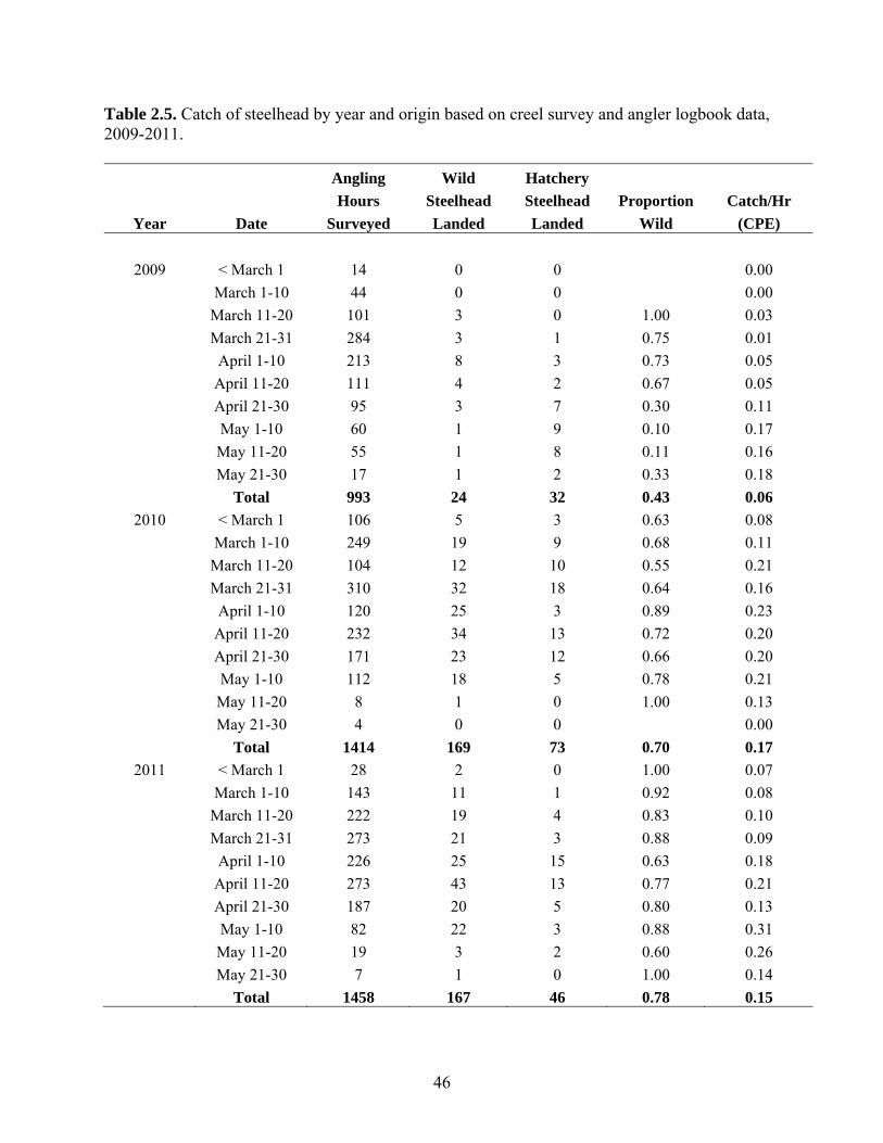
46

Table 2.5. Catch of steelhead by year and origin based on creel survey and angler logbook data, 2009-2011.

Angling Wild Hatchery

Hours Steelhead Steelhead Proportion Catch/Hr

Year Date Surveyed Landed Landed Wild (CPE)

2009 < March 1 14 0 0 0.00

March 1-10 44 0 0 0.00

March 11-20 101 3 0 1.00 0.03

March 21-31 284 3 1 0.75 0.01

April 1-10 213 8 3 0.73 0.05

April 11-20 111 4 2 0.67 0.05

April 21-30 95 3 7 0.30 0.11

May 1-10 60 1 9 0.10 0.17

May 11-20 55 1 8 0.11 0.16

May 21-30 17 1 2 0.33 0.18

Total 993 24 32 0.43 0.06

2010 < March 1 106 5 3 0.63 0.08

March 1-10 249 19 9 0.68 0.11

March 11-20 104 12 10 0.55 0.21

March 21-31 310 32 18 0.64 0.16

April 1-10 120 25 3 0.89 0.23

April 11-20 232 34 13 0.72 0.20

April 21-30 171 23 12 0.66 0.20

May 1-10 112 18 5 0.78 0.21

May 11-20 8 1 0 1.00 0.13

May 21-30 4 0 0 0.00

Total 1414 169 73 0.70 0.17

2011 < March 1 28 2 0 1.00 0.07

March 1-10 143 11 1 0.92 0.08

March 11-20 222 19 4 0.83 0.10

March 21-31 273 21 3 0.88 0.09

April 1-10 226 25 15 0.63 0.18

April 11-20 273 43 13 0.77 0.21

April 21-30 187 20 5 0.80 0.13

May 1-10 82 22 3 0.88 0.31

May 11-20 19 3 2 0.60 0.26

May 21-30 7 1 0 1.00 0.14

Total 1458 167 46 0.78 0.15

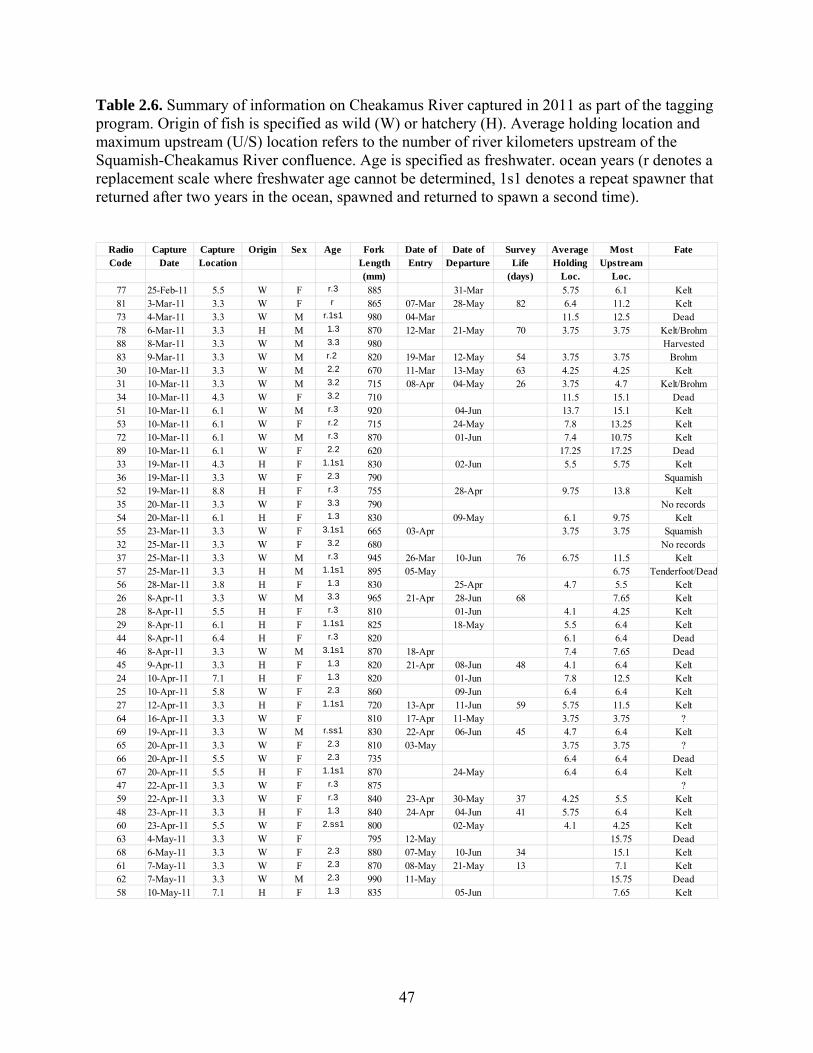
47

Table 2.6. Summary of information on Cheakamus River captured in 2011 as part of the tagging program. Origin of fish is specified as wild (W) or hatchery (H). Average holding location and maximum upstream (U/S) location refers to the number of river kilometers upstream of the Squamish-Cheakamus River confluence. Age is specified as freshwater. ocean years (r denotes a replacement scale where freshwater age cannot be determined, 1s1 denotes a repeat spawner that returned after two years in the ocean, spawned and returned to spawn a second time).

Radio Capture Capture Origin Sex Age Fork Date of Date of Survey Average Most FateCode Date Location Length Entry Departure Life Holding Upstream

(mm) (days) Loc. Loc.77 25-Feb-11 5.5 W F r.3 885 31-Mar 5.75 6.1 Kelt81 3-Mar-11 3.3 W F r 865 07-Mar 28-May 82 6.4 11.2 Kelt73 4-Mar-11 3.3 W M r.1s1 980 04-Mar 11.5 12.5 Dead78 6-Mar-11 3.3 H M 1.3 870 12-Mar 21-May 70 3.75 3.75 Kelt/Brohm88 8-Mar-11 3.3 W M 3.3 980 Harvested83 9-Mar-11 3.3 W M r.2 820 19-Mar 12-May 54 3.75 3.75 Brohm30 10-Mar-11 3.3 W M 2.2 670 11-Mar 13-May 63 4.25 4.25 Kelt31 10-Mar-11 3.3 W M 3.2 715 08-Apr 04-May 26 3.75 4.7 Kelt/Brohm34 10-Mar-11 4.3 W F 3.2 710 11.5 15.1 Dead51 10-Mar-11 6.1 W M r.3 920 04-Jun 13.7 15.1 Kelt53 10-Mar-11 6.1 W F r.2 715 24-May 7.8 13.25 Kelt72 10-Mar-11 6.1 W M r.3 870 01-Jun 7.4 10.75 Kelt89 10-Mar-11 6.1 W F 2.2 620 17.25 17.25 Dead33 19-Mar-11 4.3 H F 1.1s1 830 02-Jun 5.5 5.75 Kelt36 19-Mar-11 3.3 W F 2.3 790 Squamish52 19-Mar-11 8.8 H F r.3 755 28-Apr 9.75 13.8 Kelt35 20-Mar-11 3.3 W F 3.3 790 No records54 20-Mar-11 6.1 H F 1.3 830 09-May 6.1 9.75 Kelt55 23-Mar-11 3.3 W F 3.1s1 665 03-Apr 3.75 3.75 Squamish32 25-Mar-11 3.3 W F 3.2 680 No records37 25-Mar-11 3.3 W M r.3 945 26-Mar 10-Jun 76 6.75 11.5 Kelt57 25-Mar-11 3.3 H M 1.1s1 895 05-May 6.75 Tenderfoot/Dead56 28-Mar-11 3.8 H F 1.3 830 25-Apr 4.7 5.5 Kelt26 8-Apr-11 3.3 W M 3.3 965 21-Apr 28-Jun 68 7.65 Kelt28 8-Apr-11 5.5 H F r.3 810 01-Jun 4.1 4.25 Kelt29 8-Apr-11 6.1 H F 1.1s1 825 18-May 5.5 6.4 Kelt44 8-Apr-11 6.4 H F r.3 820 6.1 6.4 Dead46 8-Apr-11 3.3 W M 3.1s1 870 18-Apr 7.4 7.65 Dead45 9-Apr-11 3.3 H F 1.3 820 21-Apr 08-Jun 48 4.1 6.4 Kelt24 10-Apr-11 7.1 H F 1.3 820 01-Jun 7.8 12.5 Kelt25 10-Apr-11 5.8 W F 2.3 860 09-Jun 6.4 6.4 Kelt27 12-Apr-11 3.3 H F 1.1s1 720 13-Apr 11-Jun 59 5.75 11.5 Kelt64 16-Apr-11 3.3 W F 810 17-Apr 11-May 3.75 3.75 ?69 19-Apr-11 3.3 W M r.ss1 830 22-Apr 06-Jun 45 4.7 6.4 Kelt65 20-Apr-11 3.3 W F 2.3 810 03-May 3.75 3.75 ?66 20-Apr-11 5.5 W F 2.3 735 6.4 6.4 Dead67 20-Apr-11 5.5 H F 1.1s1 870 24-May 6.4 6.4 Kelt47 22-Apr-11 3.3 W F r.3 875 ?59 22-Apr-11 3.3 W F r.3 840 23-Apr 30-May 37 4.25 5.5 Kelt48 23-Apr-11 3.3 H F 1.3 840 24-Apr 04-Jun 41 5.75 6.4 Kelt60 23-Apr-11 5.5 W F 2.ss1 800 02-May 4.1 4.25 Kelt63 4-May-11 3.3 W F 795 12-May 15.75 Dead68 6-May-11 3.3 W F 2.3 880 07-May 10-Jun 34 15.1 Kelt61 7-May-11 3.3 W F 2.3 870 08-May 21-May 13 7.1 Kelt62 7-May-11 3.3 W M 2.3 990 11-May 15.75 Dead58 10-May-11 7.1 H F 1.3 835 05-Jun 7.65 Kelt

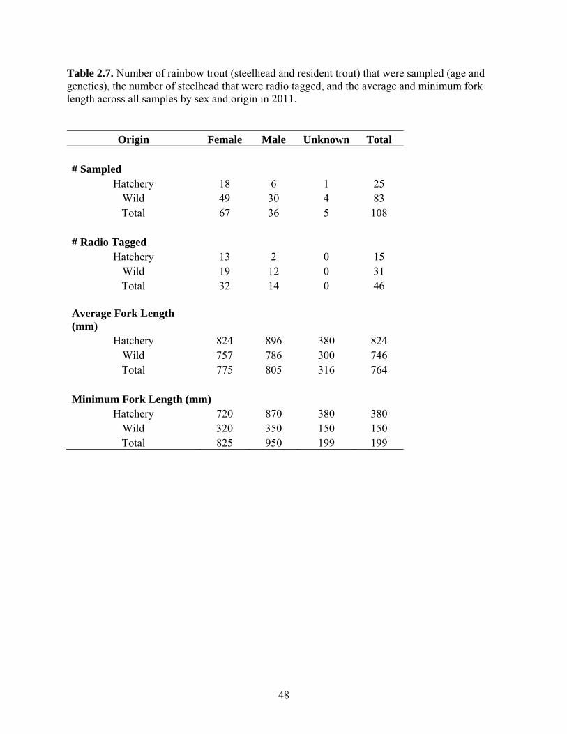
48

Table 2.7. Number of rainbow trout (steelhead and resident trout) that were sampled (age and genetics), the number of steelhead that were radio tagged, and the average and minimum fork length across all samples by sex and origin in 2011.

Origin Female Male Unknown Total

# Sampled Hatchery 18 6 1 25

Wild 49 30 4 83 Total 67 36 5 108

# Radio Tagged Hatchery 13 2 0 15

Wild 19 12 0 31 Total 32 14 0 46

Average Fork Length (mm)

Hatchery 824 896 380 824 Wild 757 786 300 746 Total 775 805 316 764

Minimum Fork Length (mm) Hatchery 720 870 380 380

Wild 320 350 150 150 Total 825 950 199 199

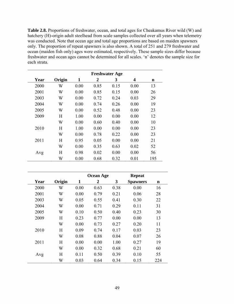
49

Table 2.8. Proportions of freshwater, ocean, and total ages for Cheakamus River wild (W) and hatchery (H)-origin adult steelhead from scale samples collected over all years when telemetry was conducted. Note that ocean age and total age proportions are based on maiden spawners only. The proportion of repeat spawners is also shown. A total of 251 and 279 freshwater and ocean (maiden fish only) ages were estimated, respectively. These sample sizes differ because freshwater and ocean ages cannot be determined for all scales. ‘n’ denotes the sample size for each strata.

Freshwater Age Year Origin 1 2 3 4 n 2000 W 0.00 0.85 0.15 0.00 13 2001 W 0.00 0.85 0.15 0.00 26 2003 W 0.00 0.72 0.24 0.03 29 2004 W 0.00 0.74 0.26 0.00 19 2005 W 0.00 0.52 0.48 0.00 23 2009 H 1.00 0.00 0.00 0.00 12

W 0.00 0.60 0.40 0.00 10 2010 H 1.00 0.00 0.00 0.00 23

W 0.00 0.78 0.22 0.00 23 2011 H 0.95 0.05 0.00 0.00 21

W 0.00 0.35 0.63 0.02 52 Avg H 0.98 0.02 0.00 0.00 56

W 0.00 0.68 0.32 0.01 195

Ocean Age Repeat Year Origin 1 2 3 Spawners n 2000 W 0.00 0.63 0.38 0.00 16 2001 W 0.00 0.79 0.21 0.06 28 2003 W 0.05 0.55 0.41 0.30 22 2004 W 0.00 0.71 0.29 0.11 31 2005 W 0.10 0.50 0.40 0.23 30 2009 H 0.23 0.77 0.00 0.00 13

W 0.00 0.73 0.27 0.20 11 2010 H 0.09 0.74 0.17 0.03 23

W 0.08 0.88 0.04 0.07 26 2011 H 0.00 0.00 1.00 0.27 19

W 0.00 0.32 0.68 0.21 60 Avg H 0.11 0.50 0.39 0.10 55

W 0.03 0.64 0.34 0.15 224

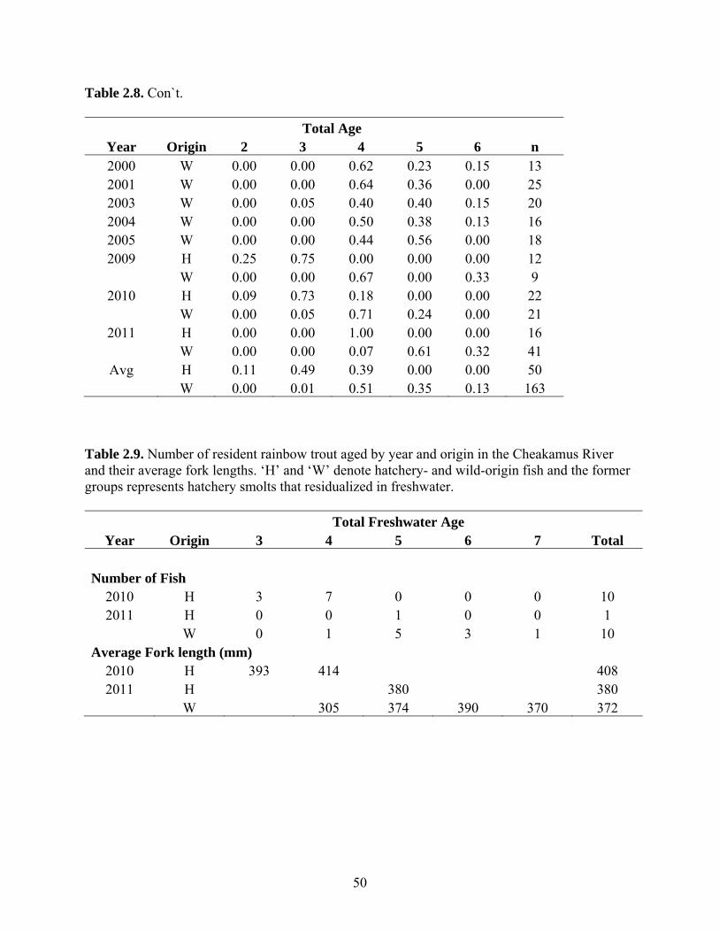
50

Table 2.8. Con`t.

Total Age Year Origin 2 3 4 5 6 n 2000 W 0.00 0.00 0.62 0.23 0.15 13 2001 W 0.00 0.00 0.64 0.36 0.00 25 2003 W 0.00 0.05 0.40 0.40 0.15 20 2004 W 0.00 0.00 0.50 0.38 0.13 16 2005 W 0.00 0.00 0.44 0.56 0.00 18 2009 H 0.25 0.75 0.00 0.00 0.00 12

W 0.00 0.00 0.67 0.00 0.33 9 2010 H 0.09 0.73 0.18 0.00 0.00 22

W 0.00 0.05 0.71 0.24 0.00 21 2011 H 0.00 0.00 1.00 0.00 0.00 16

W 0.00 0.00 0.07 0.61 0.32 41 Avg H 0.11 0.49 0.39 0.00 0.00 50

W 0.00 0.01 0.51 0.35 0.13 163 Table 2.9. Number of resident rainbow trout aged by year and origin in the Cheakamus River and their average fork lengths. ‘H’ and ‘W’ denote hatchery- and wild-origin fish and the former groups represents hatchery smolts that residualized in freshwater.

Total Freshwater Age Year Origin 3 4 5 6 7 Total

Number of Fish 2010 H 3 7 0 0 0 10 2011 H 0 0 1 0 0 1

W 0 1 5 3 1 10 Average Fork length (mm)

2010 H 393 414 408 2011 H 380 380

W 305 374 390 370 372

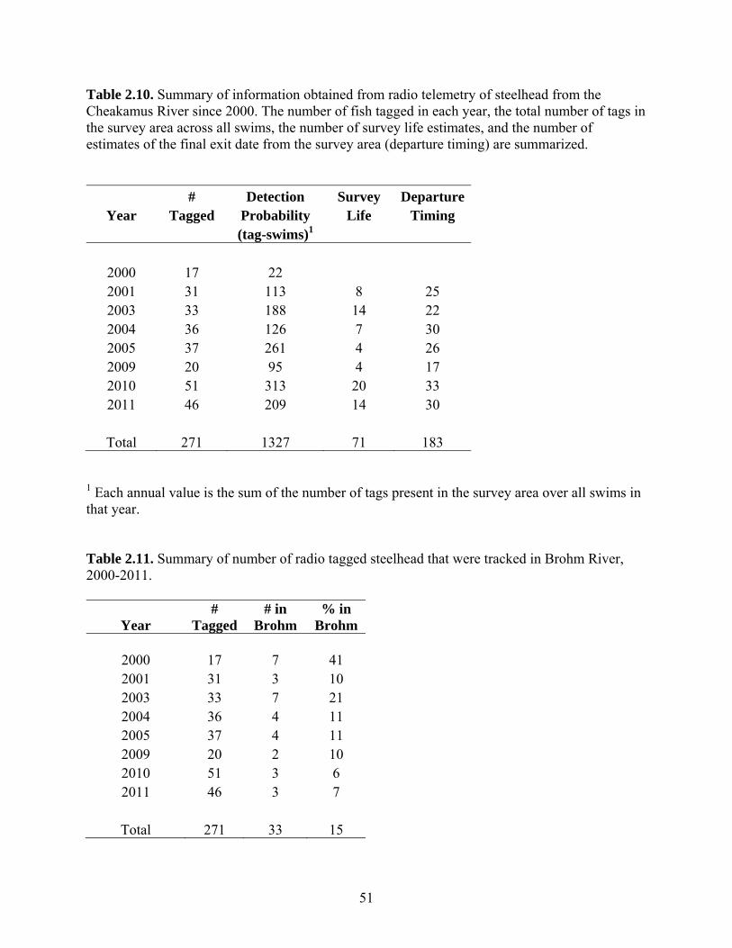
51

Table 2.10. Summary of information obtained from radio telemetry of steelhead from the Cheakamus River since 2000. The number of fish tagged in each year, the total number of tags in the survey area across all swims, the number of survey life estimates, and the number of estimates of the final exit date from the survey area (departure timing) are summarized.

# Detection Survey DepartureYear Tagged Probability Life Timing

(tag-swims)1

2000 17 22 2001 31 113 8 25 2003 33 188 14 22 2004 36 126 7 30 2005 37 261 4 26 2009 20 95 4 17 2010 51 313 20 33 2011 46 209 14 30

Total 271 1327 71 183 1 Each annual value is the sum of the number of tags present in the survey area over all swims in that year. Table 2.11. Summary of number of radio tagged steelhead that were tracked in Brohm River, 2000-2011.

Year #

Tagged # in

Brohm % in

Brohm

2000 17 7 41 2001 31 3 10 2003 33 7 21 2004 36 4 11 2005 37 4 11 2009 20 2 10 2010 51 3 6 2011 46 3 7

Total 271 33 15

52

Table 2.12. Comparison of four linear models predicting survey life as a function of date of entry into the survey area based on alternate stratification schemes (unstratified, sex-stratified, year-stratified, and origin-stratified). b0 and b1 represent the constant and slope of the relationship, while n and K represents the sample size and number of parameters in the mode, respectively. LL, AIC, and AIC are the log-likelihood, Akaikie Information Criteria statistic, and the difference in AIC relative to the model with the lowest AIC score, respectively. ‘M’, ‘F’, “W”, and “H”denote males, females, wild-origin, and hatchery-origin steelhead, respectively. Note the model with the lowest AIC score is considered to be the most reliable. There is little support for models with AIC scores > 7 relative to the model with the lowest score.

Model Sex Year Origin b0 b1 n K LL AIC AIC

1 No No No 100.58 -0.58 71 2 -295 593 6

2 M No No 113.29 -0.65 34 4 -289 587 0 F 93.41 -0.56 37

3 No 2001 No 111.68 -0.64 8 14 -284 597 10 2003 117.15 -0.83 14 2004 80.14 -0.34 7 2005 109.87 -0.76 4 2009 38.53 0.06 4 2010 56.92 -0.19 20 2011 120.21 -0.70 14

4 No No W 104.23 -0.63 9 4 -293 594 7 H 90.03 -0.41 62

53

Table 2.13. Comparison of models predicting departure date. The median exit date represents the date when 50% of the tagged fish have migrated downstream out of the survey area (downstream of the Cheekye confluence). n, K, LL, AIC, and AIC are the sample size, number of parameters in the model, log-likelihood, Akaikie Information Criteria statistic, and the difference in AIC relative to the model with the lowest AIC score, respectively. ‘M’, ‘F’, ‘W’, and ‘H’ denote males, females, wild-origin, and hatchery-origin fish, respectively. Note the model with the lowest AIC score is considered to be the most reliable. There is little support for models with AIC scores > 7 relative to the model with the lowest score.

MedianExit

Model Sex Origin Year Date n LL K AIC AIC

1 No No No 18-May 183 -778 2 1559 392

2 M No No 22-May 80 -326 4 1481 314 F 15-May 103 -411

3 No W 17-May 154 -652 4 1505 338 H 26-May 29 -97

4 No No 2001 11-May 25 -79 14 1232 65 2003 05-May 22 -76 2004 19-May 30 -100 2005 13-May 26 -78 2009 23-May 17 -47 2010 25-May 33 -119 2011 21-May 30 -104

5 No W 2001 11-May 25 -79 20 1167 0 2003 05-May 22 -76 2004 19-May 30 -100 2005 13-May 26 -78 2009 21-May 14 -37 2010 22-May 20 -65 2011 19-May 17 -55

H 2009 28-May 3 -3 2010 26-May 13 -34 2011 21-May 13 -36

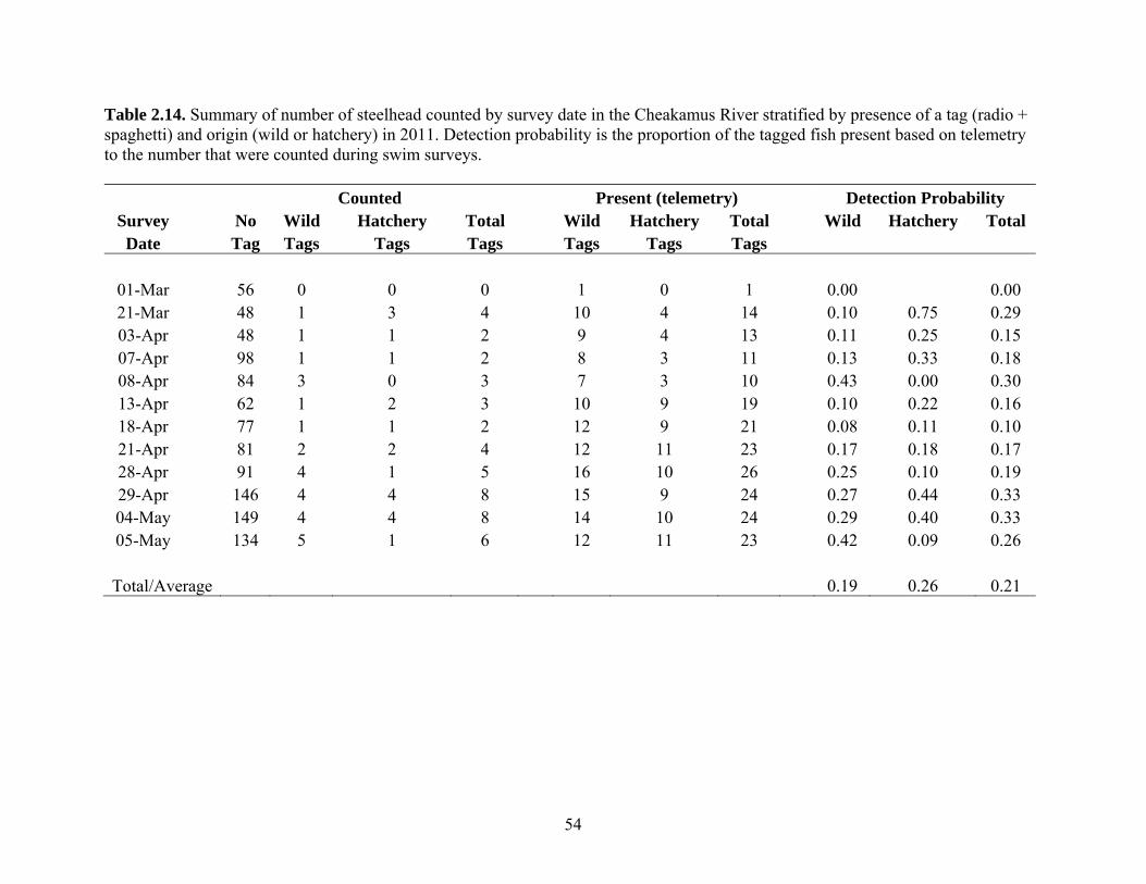
54

Table 2.14. Summary of number of steelhead counted by survey date in the Cheakamus River stratified by presence of a tag (radio + spaghetti) and origin (wild or hatchery) in 2011. Detection probability is the proportion of the tagged fish present based on telemetry to the number that were counted during swim surveys.

Counted Present (telemetry) Detection Probability Survey No Wild Hatchery Total Wild Hatchery Total Wild Hatchery Total Date Tag Tags Tags Tags Tags Tags Tags

01-Mar 56 0 0 0 1 0 1 0.00 0.00 21-Mar 48 1 3 4 10 4 14 0.10 0.75 0.29 03-Apr 48 1 1 2 9 4 13 0.11 0.25 0.15 07-Apr 98 1 1 2 8 3 11 0.13 0.33 0.18 08-Apr 84 3 0 3 7 3 10 0.43 0.00 0.30 13-Apr 62 1 2 3 10 9 19 0.10 0.22 0.16 18-Apr 77 1 1 2 12 9 21 0.08 0.11 0.10 21-Apr 81 2 2 4 12 11 23 0.17 0.18 0.17 28-Apr 91 4 1 5 16 10 26 0.25 0.10 0.19 29-Apr 146 4 4 8 15 9 24 0.27 0.44 0.33 04-May 149 4 4 8 14 10 24 0.29 0.40 0.33 05-May 134 5 1 6 12 11 23 0.42 0.09 0.26

Total/Average 0.19 0.26 0.21

55

Table 2.15. Comparison of detection probability models for steelhead in the Cheakamus River without (model 1) and with (model 2) stratification by fish origin (“H” = hatchery, “W”= wild) based on data from 2009, 2010, and 2011. b0 represents detection probability, while # of tag-swims represents the cumulative number of tags present across swims. LL, AIC, and AIC are the log-likelihood, Akaikie Information Criteria statistic, and the difference in AIC relative to the model with the lowest AIC score, respectively. The model with the lowest AIC score is considered to be the most reliable.

# of tag Model Origin b0 -swims K LL AIC AIC

1 No 0.19 617 1 -104 209 0

2 H 0.20 209 2 -104 211 2 W 0.19 408

Table 2.16. Comparison of two logistic models predicting detection probability as a function of the ratio of horizontal visibility to discharge. b0 and b1 represent the constant and slope of the relationship, while n and K represents the sample size and number of parameters in the model (twice as many for model 2 where 2 sets of b0 and b1 values are estimated). LL, AIC, and AIC are the log-likelihood, Akaikie Information Criteria statistic, and the difference in AIC relative to the model with the lowest AIC score, respectively. The model with the lowest AIC score is considered to be the most reliable. There is little support for models with AIC scores > 7 relative to the model with the lowest score.

Model Year b0 b1 n K LL AIC AIC

1 2000-2011 0.53 1.38 90 2 -171 345 24

2 2000-2005 0.35 1.80 52 4 -157 322 0 2009-2011 0.37 3.66 38

56

Table 2.17. Calculations used to estimate annual egg deposition for steelhead in the Cheakamus River in years when information on sex ratio and size is available from angling surveys. Egg deposition is computed as the product of escapement, the proportion females, and fecundity. The latter estimates are computed based on mean female fork length and a fecundity-fork length relationship from the Keogh River (Ward and Slaney 1993).

Fork length Average Total Egg ('000s) -& Sex Female Fork Average Proportion Total Eggs Escapement

Year Sample Size Length (mm) Fecundity Females Escapement ('000s) Ratio

2000 18 700 3,329 0.50 103 171 1.7 2001 27 756 4,219 0.41 310 533 1.7 2003 33 801 5,016 0.52 311 804 2.6 2004 36 769 4,431 0.44 330 650 2.0 2005 38 776 4,552 0.50 332 756 2.3 2009 27 735 3,864 0.59 204 467 2.3 2010 57 691 3,206 0.44 1,144 1,609 1.4 2011 107 794 4,885 0.61 1,071 3,178 3.0

57

Table 2.18. Return rate for the hatchery-origin steelhead smolts released into the Cheakamus River in 2007 and 2008. Return rate is computed by dividing the total hatchery origin escapement from each release year by the number of smolts released. Hatchery escapement estimates by return year are assigned to release year based on the proportion of ocean age 1, 2, and 3 yr fish in the hatchery-origin escapement determined by ageing. Number of Hatchery Smolts Released

Release Year Total 2007 21,505 2008 17,618

Hatchery Returns Return Year 2009 2010 2011

Escapement (return yr only) 101 436 347

Hatchery age composition Ocean age 1 0.23 0.00 0.00 Ocean age 2 0.77 0.74 0.00 Ocean age 3 0.00 0.17 1.00

Escapement (release x return yr) Total 2007 78 83 0 161 2008 23 353 347 723

Hatchery Return Rate Release Year Total

2007 0.75% 2008 4.11%

58

Table 2.19. Calculations used to compare estimated smolt production at the Rotary Screw Trap (RST) on the Cheakamus River in 2008 with a back-calculated estimate of smolt production based on adult returns by ocean age and an estimated marine survival rate for wild fish. Marine survival from relase to southern Howe Sounds (POST)1

Wild 68% Hatchery 27%

Wild-to-hatchery survival rate 2.5

estimated return rate of 2008 hatchery-origin smolts 4.1% Calculated marine survival for 2008 wild-origin smolts 10.3%

Estimated wild-origin escapement from 2008 outmigrants 2010 returns (ocean age 2) 626 2011 returns (ocean age 3) 495

Total 1,121

Back-calculated wild-origin smolts in 2008 10,843

Estimated wild-origin smolts at RST in 20082 6,617 Upper Paradise smolt production in 20082 193 Total smolt production above the RST 6,810

1Melnychuck et al. 2009. 2Melville and McCubbing 2009.

59

Table 2.20. Summary of steelhead escapement estimates to Brohm River in 2010 and 2011 based on the resistivity counter, redd counts, and calculations that depend on escapement in the Cheakamus River and the immigration rate into Brohm River based on radio tags.

2010 2011 Brohm Escapement

Resistivity Counter 65 54 Redd Counts 70 70

Derived Brohm Escapement Cheakamus Escapement

Wild 708 724 Total 1144 1071

Brohm Immigration Rate 5.9% 6.5%

Escapement to Brohm River based on Wild 42 47 based on Total 67 70

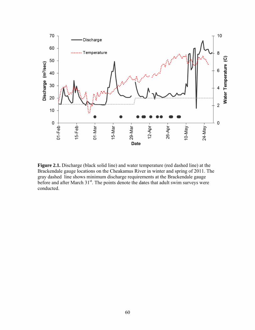
FigurBrackgray beforcondu

re 2.1. Dischkendale gaugdashed line

re and after Mucted.

harge (blackge locations shows miniMarch 31st. T

k solid line) aon the Chea

imum dischaThe points d

60

and water temakamus Rivearge requiremdenote the da

mperature (rer in winter aments at the ates that adul

red dashed liand spring oBrackendalelt swim surv

ine) at the of 2011. The e gauge

veys were

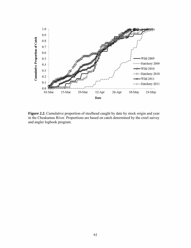
Figurin theand a

re 2.2. Cumue Cheakamuangler logboo

ulative props River. Propok program.

ortion of steportions are

61

eelhead caugbased on ca

ght by date batch determin

y stock origned by the cr

in and year reel survey

Figurdays by seare th

re 2.3. Relatspent in the

ex and stock he best-fit lin

tionship betwsurvey area origin using

near relation

ween date of(survey life

g data from anships fit to d

62

f entry into t) for steelhe

all years whedata by sex u

the survey aread in the Chen telemetryusing data fr

rea and the nheakamus Riy was conducom both stoc

number of iver stratifiedcted. Lines cks.

d

Figurdate ffish i

re 2.4. Cumufrom 2001 thn 2011 (b).

ulative prophrough 2011

ortion of rad1 (a) and the

63

dio tagged stdeparture sc

teelhead depchedule for w

parting the suwild- and ha

urvey area byatchery-origi

y in

F

FigursnorkCheaor to are u

re 2.5. The rkel surveys aakamus Rive

2000-2005 (sed to estima

relationship and the ratio r. Lines are (gray dashedate escapem

between detof horizontabest-fit logis

d line) and 2ment.

64

tection probaal visibility (stic relations009-2011(gr

ability for ad(HV) to discships to all thray dotted li

dult steelheacharge (Q) inhe data (blacine). The latt

ad during n the ck solid line)ter models

)

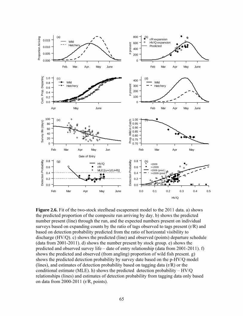
65

Figure 2.6. Fit of the two-stock steelhead escapement model to the 2011 data. a) shows the predicted proportion of the composite run arriving by day. b) shows the predicted number present (line) through the run, and the expected numbers present on individual surveys based on expanding counts by the ratio of tags observed to tags present (r/R) and based on detection probability predicted from the ratio of horizontal visibility to discharge (HV/Q). c) shows the predicted (line) and observed (points) departure schedule (data from 2001-2011). d) shows the number present by stock group. e) shows the predicted and observed survey life – date of entry relationship (data from 2001-2011). f) shows the predicted and observed (from angling) proportion of wild fish present. g) shows the predicted detection probability by survey date based on the p-HV/Q model (lines), and estimates of detection probability based on tagging data (r/R) or the conditional estimate (MLE). h) shows the predicted detection probability – HV/Q relationships (lines) and estimates of detection probability from tagging data only based on data from 2000-2011 (r/R, points).

0.000

0.005

0.010

0.015 WildHatchery

Pro

port

ion

Arr

ivin

g (a)

Feb. Mar. Apr. May June

0

200

400

600

800

# pr

esen

t

r/R expansionHV/Q expansionPredicted

(b)

Feb Mar Apr May June

0.0

0.2

0.4

0.6

0.8

1.0

Cum

. Pro

p. D

epar

ting

WildHatchery

(c)

Apr May June

0

100

200

300

400

# pr

esen

t

Feb Mar Apr May June

WildHatchery

(d)

Feb Mar Apr May Jun

0

20

40

60

80

100

Date of Entry

Sur

vey

life

(day

s) (e)

Feb Mar Apr May

0.700.750.800.850.900.951.00

Pro

p. W

ild in

Cat

ch (f )

0.0

0.2

0.4

0.6

0.8

Det

ectio

n P

roba

bilit

y

HV/Qr/RMLE [(u+r)/(U+R)]

(g)

Feb Mar Apr May June 0.0 0.1 0.2 0.3 0.4 0.5

0.0

0.2

0.4

0.6

0.8

HV/Q

Det

ectio

n P

roba

bilit

y

<2009>=2009<2009 (pred.)>=2009 (pred.)

(h)

66

Figure 2.7. The steelhead escapement trend in the Cheakamus River, 1996-2011 showing abundance of returns that reared as juveniles in the river before and after the Instream Flow Agreement (IFA) was implemented and the year that the sodium hydroxide spill occurred (Post-Spill). The height of the bars and error bars show the average and 90% credible intervals from the posterior distribution of escapement estimates for each year, respectively.

0

200

400

600

800

1000

1996 1997 1999 2000 2001 2002 2003 2004 2005 2006 2007 2008 2009 2010 2011

Ste

elh

ead

Esc

apem

ent

Return Year

Wild Hatchery

Pre-IFA IFA/Pre-Spill Post-Spill

FigurCheaspawthe avrelatiit doe

re 2.8. The rakamus Rive

wners). The yverage recruionship. Notees not yet inc

relationship r and the res

year beside euitment over e that the recclude 6 year

between thesulting maideach point repthe period o

cruitment estold fish that

67

e number of sen adult retupresents the

of record andtimate for tht will return

steelhead spurns (total rebrood year.

d the dashed he 2006 brooin 2012.

pawners in theturns less re The solid li

d line represeod year is inc

he epeat ine representents the 1:1 complete as

ts

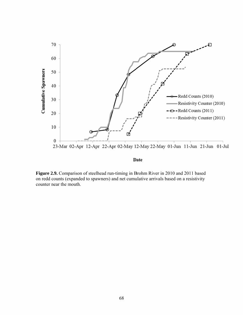
Figuron recount

re 2.9. Compdd counts (eter near the m

parison of stexpanded to mouth.

teelhead runspawners) an

68

n-timing in Bnd net cumu

Brohm River ulative arriva

r in 2010 andals based on

d 2011 baseda resistivity

d y

69

Appendix A.2. Distribution of Radio Tagged Steelhead, 2001-

2011.

This appendix presents graphical representations of the distribution of radio

tagged steelhead in the Cheakamus River based on tagging in 2001, 2003-2005, and

2009-2011. The graphics are based on an integration of data collected from fixed

telemetry stations and mobile tracking in these years. The programs Adobe Flash Player

CS3 and Adobe Illustrator CS3 with custom plug-ins were used to animate the position of

each fish in a web browser based on these data. The plots below show the positions of

each fish between tagging and when they left the system or died. The abbreviations

“SQM”, “CHE”, “BAI”, “CUL”, and “EOR” denote the location of the Squamish-

Cheakamus confluence, the Cheakamus-Cheekye confluence, the Bailey Bridge, the

Cheakamus-Culliton confluence, and the end-of-road, respectively. Each fish is identified

by its radio tag code. The red line for each fish represents its maximum range as inferred

from the fixed station and mobile survey data. Arrows denote whether a fish was tracked

moving upstream or downstream at a fixed station location.

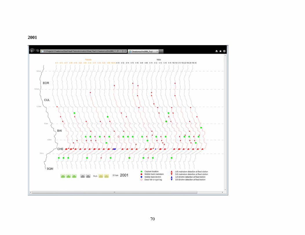
2 2001

70

22003

71

22004

72

22005

73

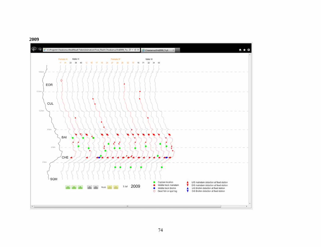
22009

74

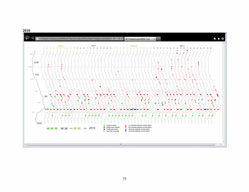
22010

75

2 2011

76

77

3.0 Juvenile Steelhead Abundance

3.1 Introduction

This section summarizes the methods and results from steelhead juvenile

abundance surveys conducted in Cheakamus and Brohm Rivers in fall 2010 and spring

2011. It also provides revised estimates of abundance from previous surveys. Changes in

juvenile abundance over multiple years can be related to changes in flow regime or other

habitat changes to make inferences about how freshwater habitat quantity and quality

effects juvenile steelhead production (Fig. 1.3b). The evaluation of habitat effects

includes assessing potential benefits and impacts of the new WUP flow regime.

Differences in the abundance within age classes between fall and spring surveys can be

used to estimate apparent survival rates between these periods. The over-winter period

(fall to spring surveys) is important to assess since flows in the Cheakamus River are

most affected by regulation from Daisy dam during periods of low inflows, which are

common during winter, and winter flow regimes have been shown to be important

determinants of juvenile salmonid production and/or mortality in some systems

(Hvidseten 1993, Bradford et al. 1995, Jensen and Johnsen 1999, Saltveit et al. 2001,

Mitro et al. 2003). The summer period (spring to fall surveys) is important because

habitat availability shortly after emergence (Elliot 1994, Nislow et al. 2004) or during

low flow periods in late summer (Berger and Gresswell 2009, Harvey at al. 2005) have

been shown to be important determinants of juvenile production as well, and most of the

hypotheses during the Cheakamus WUP for steelhead focused on effects of low flow

periods in the fall (Marmorek and Parnell 2002). Juvenile abundance can be related to

escapement via estimation of life-stage specific stock-recruitment relationships so

density-dependent effects can be accounted for when interpreting changes in juvenile

abundance and survival through time (Fig. 1.3c). Estimates of juvenile abundance in

Brohm and Cheakamus River can be compared to determine what fraction of the

aggregated population rears in Brohm River, which is not effected by flow regulation

from Daisy Dam.

The evaluation of the effects of habitat, flow, and escapement on juvenile

abundance and survival can only be accomplished with a relatively long-term dataset.

78

The juvenile component of this project began in fall 2007 (Korman 2008) and only four

years of juvenile abundance data are available (Fig. 1.4). Sampling for juvenile steelhead

prior to 2007 has been limited and based on the non-random selection of sites thought to

contain high quality parr habitat (see review in Van Dishoeck 2000). Changes in

abundance estimates from such studies are unlikely to reflect river-wide changes in

abundance because many factors, including variation in juvenile density, will affect

patterns of habitat use (Bohlin 1978, Rosenfeld and Boss 2001, Girard et al. 2004,

Rosenfeld et al. 2005, Gibson et al. 2008). The outmigrant trapping program has

enumerated steelhead smolts since 2000, but estimates of steelhead smolt outmigration

abundance are available for only a subset of these years, and uncertainty in these

estimates may be significantly underestimated due to logistical and analytical challenges

(Melville and McCubbing 2011). Given these historical difficulties and limitations, the

emphasis of our analysis of the juvenile data collected in the early phases of this project

focuses on evaluating potential bias and the precision of abundance estimates. In year 1,

we investigated a variety of sampling techniques (Korman 2008), which guided the

sampling design of the intensive program initiated in year 2. In this chapter, we report on

the results from surveys conducted in year 4. A key assumption in our methodology is

that data on detection probability of juvenile steelhead based on mark-recapture

experiments is exchangeable among years. We combine data from mark-recapture

experiments across years using a hierarchical Bayesian model (HBM) to compute year-

specific abundance estimates. Thus, previously published juvenile abundance estimates

for the Cheakamus and Brohm Rivers (fall 2008, 2009 and spring 2009, 2010 estimates

from Korman et al. 2011) must be updated to reflect the addition of fall 2010 and spring

2011 mark-recapture data. Given the additional mark-recapture data, this chapter includes

revised values for previously published estimates (Korman et al. 2011).

3.2 Methods We used a multi-gear two-phase sampling design to estimate the abundance of

age 0-, 1-, and 2-yr old juvenile steelhead in the Cheakamus and Brohm Rivers. We first

conducted habitat surveys in both systems to quantify the length of shoreline that was

potentially useable by juvenile steelhead. In the Cheakamus River, we classified useable

shoreline habitat into riffle, shallow, and deep habitat types (see section 3) and used

79

different gears to sample these types depending on season (fall or spring) and age. Gear

stratification was based on the depth limitations of the sampling gear (snorkeling not

possible in riffles, electrofishing difficult and inefficient in deep habitat types), seasonal

gear restrictions (snorkeling not possible in fall due to high turbidity), and previous

evaluations of the habitat and life stage-specific effectiveness of each gear (Korman

2008, Korman et al. 2011) which showed that electrofishing provides the most unbiased

and precise estimates of age 0 abundance in habitat types where the gear can be applied,

while snorkeling provides the most unbiased and precise estimates of abundance for age

1 and older juvenile steelhead (hereafter referred to as parr or age 1+ fish). In addition,

the top priority of the juvenile program is to estimate the abundance of steelhead parr in

the spring prior to outmigration, given the need to provide a reliable index of freshwater

juvenile production. Given these various constraints, statistical considerations and

priorities, fall estimates of abundance were based exclusively on electrofishing (Table

3.1). Spring abundance estimates were based on data from both electrofishing and snorkel

surveys. For estimates of age 0 abundance, we used data from riffle and shallow sites

sampled by electrofishing, and deep sites sampled by snorkeling. For estimates of age 1+

juvenile steelhead, we used data from riffle and shallow sites sampled by electrofishing,

and shallow and deep sites sampled by snorkeling.

Abundance was estimated using a two-phase sampling design. We sampled a

large number of index sites using a single pass of effort. At a sub-sample of sites, we

conducted two-day mark-recapture experiments to quantify detection probability. We

define detection probability as the proportion of individuals at a site that are either

captured by electrofishing or seen by a diver based on a single pass of effort. Abundance

at index sites was estimated by expanding the observed number of fish by the estimates

of detection probability determined from mark-recapture experiments. The abundance of

fish in the shorelines that were not sampled was estimated based on average fish densities

and variation in density across sampled sites. The total estimate of abundance for the

river was the sum of estimates from sampled and unsampled shorelines. We developed a

Hierarchical Bayesian Model (HBM) to implement this approach to estimate posterior

distributions of abundance, from which expected values (means), medians, and 95%

credible intervals could be computed.

80

3.2.1 SampleSiteSelectionandFieldMethodsA total of 18 and 99 index sites were electrofished (EF) for the fall 2010

abundance estimates in the Brohm and Cheakamus Rivers, respectively (Table 3.1). A

total of 2 and 5 mark-recapture experiments were completed in fall 2010 in the Brohm

and Cheakamus Rivers, respectively. A total of 20 and 203 index sites were sampled in

spring 2011 using either electrofishing and snorkeling in Brohm and Cheakamus Rivers,

respectively. In addition, we conducted 6 electrofishing and one snorkel-based mark-

recapture experiment in Brohm River in spring 2011.

Sample sites for the surveys were selected at random based on information in the

habitat survey database. The database includes a list of coordinates for the entire

shoreline in the Cheakamus and Brohm Rivers at an interval of 10 m. After excluding

unusable habitat and habitat that cannot be safely accessed (only 7% of total), we used an

Excel program to randomly select points that determined our index sampling locations.

For the spring survey, EF locations were restricted to riffle and shallow habitat types

while SN locations were restricted to shallow and deep habitat types. In the fall survey

when only electrofishing was conducted, sampling points were drawn from all habitat

types. The coordinates of the randomly selected sites were uploaded to GPS units and a

list of the habitat units to be sampled was compiled. This information was used to locate

the sites in the field. The coordinates represented the midpoint of the sample sites.

Electrofishing and snorkeling index sites were 30 and 50 m long, respectively.

Electrofishing sites were sampled during the day by a two-person crew using a model

12B Smith-Root electrofisher (settings: 300V, frequency and pulse I4-J5). Each site was

sampled by methodically traversing the site in an upstream direction and capturing all

fish that were observed. Sites were not enclosed, and sampling was conducted as far into

the thalweg as safely possible, or from bank to bank when sampling in side-channels and

narrower braids. We followed the method of Decker et al. (2009) for snorkel surveys. A

single diver traversed the site in an upstream direction searching for fish with the aid of

an underwater light. Snorkeling sites were sampled only at night, beginning 1 hr after

sunset. Divers recorded the species, fork length (to the nearest 5 mm for fish < 100 mm,

and to 10 mm for fish > 100 mm) for all fish that were observed within the site.

81

We continued to test our ability to predict whether a given index site would have

high or low juvenile steelhead densities. If such a classification was reliable and could be

done with limited effort, it would be possible to classify the entire shoreline length in

greater detail than the current approach (which determines whether a shoreline can

potentially support juvenile steelhead or not). The more detailed classification of

shorelines potentially included in the fish sample (i.e, can support juvenile fish habitat)

could in turn be used to stratify our sampling effort, allowing us to use more effort at high

density sites, ultimately leading to an improvement in the precision of total population

estimates. We assumed that the variation in density of juvenile steelhead across sites

would largely be determined by the variation in habitat quality. Our classification used to

segregate poor and good quality habitat for age 0 (fry) and age 1+ (parr) steelhead was

based on a visual assessment of depth, velocity, and cover. For age 0 steelhead, sites were

classified as ‘good’ fry habitat if over 50% of the site area was comprised of shallow

depth (< 0.5 m), low velocity (<0.2 m/s) and where cover was present in the form of

interstitial spaces between cobbles. For age 1+ steelhead, sites were classified as ‘good’

parr habitat if over 50% of the site was comprised of low velocity area and where cover

in the form of interstitial spaces, boulders, or large woody debris was present. We

compared the number of fish detected at index sites across sites classified as ‘poor’ or

‘good’ habitat for both age 0 and 1+ steelhead.

Mark-recapture experiments were conducted over a two-night period. On the first

night, fish were captured for marking by backpack electrofishing (at electrofishing sites)

or by snorkeling with dip nets (at snorkel sites). Fish were identified to species and

measured, and juvenile steelhead were marked and released back into the site. We

returned to the site 24-hours later to conduct the second sampling event using the same

gear, where the number and fork length of marked and unmarked fish was determined.

Due to relatively low fish densities, mark-recapture sites were generally at least twice as

long as index sites (> 100 m). We attempted to mark a minimum of 20 age 0 and 20 age

1+ steelhead at each site. Sample sizes generally exceeded these targets for most gear-age

combinations.

We followed the method of Decker et al. (2009) for snorkel mark-recapture

experiments. During the first sampling event, a single diver traversed the site in an

82

upstream direction searching for fish with the aid of underwater lights affixed to forearm

and mask strap. This left the diver’s hands free to use two 27 x 27 cm aquarium nets

affixed to 80 cm handles to capture fish. The diver moved through the site slowly and

methodically to avoid chasing fish from their holding locations. In near-shore areas too

shallow to search from an underwater position, the diver searched for and captured fish

by walking slowly through the habitat. At the time of capture, fish were handed to a

second crew member standing nearby who immediately measured fork length, removed a

scale in some cases for ageing, and tagged the fish. Fish were not anaesthetized because

of uncertainty about behavioral effects of the anesthetic. Immediately following marking,

fish were returned to the original lie they had been holding in prior to capture. We were

unable to acquire suitable commercially made tags for this application so manufactured

our own. These consisted of a 10-15 mm-long piece of colored chenille attached to a size

16-20 barbed, fine wire fishhook with a short (3-4 mm) length of heat-shrink tubing. Tags

were inserted by placing the hook shallowly at the posterior insertion of the dorsal fin.

We used methods developed by Korman et al. (2009) for electrofishing-based

mark-recapture experiments. A two-person crew, using a Smith-Root 12b electrofisher

(settings: 300V, frequency and pulse I4-J5), traversed the site in an upstream direction.

Electrofishing was very methodical, requiring 0.75-1.5 hrs of effort to sample each site.

After electrofishing, fish were anesthetized using clove oil and fork lengths were

measured to the nearest mm. Fish were marked using red biological dye (fall) or a small

caudal fin clip (spring). Dying is a more efficient method for marking many small fish

that are commonly captured in the fall, but the dye can result in behavioral changes or

mortality at very low water temperatures in the spring. For dying, fish were placed in an

aerated bucket with neutral red biological stain (2 g per 15 L, Sigma-Aldrich Ltd.) for 20

minutes and then transferred to aerated buckets of clear water to recover. The fork

lengths of the very small proportion of dead fish and those that were not actively

swimming after processing were recorded so they could be excluded from the count of

marked fish released into the site. The remaining fish were released throughout the

sample site, avoiding areas with high water velocity and areas within 5 m from the

upstream and downstream boundaries of the site. We felt this release strategy provided a

more suitable environment for recovery and would minimize emigration from the site if

83

fish were disoriented or unable to maintain their position immediately following release.

We assumed that marked fish would resume an undisturbed distribution within the site

before the second sampling event 24-hours later.

We returned to mark-recapture sites for the second sampling event 24-hours after

the first sampling event and recorded the number of fish by species, their sizes, and

whether the fish was marked. During the recapture events we used the same techniques

and level of effort applied at single pass index sites to ensure that detection probabilities

at mark-recapture sites would represent values encountered at index sites. At snorkel

sites, divers also sampled 25 m upstream and downstream of the mark-recapture site to

record the number and size of marked fish that had emigrated. This sampling allowed us

to evaluate the assumption that populations within mark-recapture sites can be treated as

effectively closed for the 24-hour period between sampling events. Water temperature

was recorded at all mark-recapture sites with a hand-held electronic thermometer and at

all sampling sites in Brohm River. Continuous recording temperature loggers recorded

temperature at the ‘stables area’ downstream of the Cheekye River confluence.

Horizontal visibility was measured at snorkel mark-recapture sites as the maximum

distance a diver could detect a dark submerged object.

A fish length-stratified random sampling approach was use to collect scales for

freshwater age determination. Age determinations were made for 65 and 71 juvenile

steelhead from the Brohm and Cheakamus Rivers in fall 2010, respectively, and from 92

and 123 fish from the Brohm and Cheakamus Rivers in spring 2011, respectively. Scales

were taken from a location approximately 2-4 rows above the lateral line and between the

back of the dorsal fin and the origin of the anal fin. Scales from individual fish were

mounted on standard glass microscope slides and viewed under 47x magnification using

a microfiche reader. Regions of closely spaced circuli on the scale were identified as

annuli (i.e., winter growth ‘checks’). We designate fish age relative to the time from

emergence, which for Cheakamus River steelhead occurs in July and August. Thus fish

captured in their first fall and spring since emergence are given an age class designation

of 0+, while fish capture in their second fall and spring are designated as 1+. Note this

convention differs from the one where juvenile age is determined by the number of

winters spent in freshwater. Under this designation, which is used in reporting of the

84

Cheakamus outmigrant data, fish we classify as age 0+ and 1+ in the spring sample

would be one- and two-years old (one and two winters), respectively.

3.2.2 Analytical Methods We developed a hierarchical Bayesian model (HBM) similar to model I of Wyatt

(2003 and 2002) to estimate juvenile steelhead abundance. The model consists of two

levels or hierarchies (Fig. 3.1). Site-specific estimates of detection probability and fish

density at the lowest level of the hierarchy are considered random variables that come

from hyper-distributions of detection probability and density at the higher level. The

HBM jointly estimates both site- and hyper-parameters. The process component of the

model assumes that variation in juvenile abundance across sample sites follows a

Poisson/log-normal mixture. That is, abundance at-a-site is Poisson-distributed based on

a mean density drawn from a lognormal distribution. The observation component of the

model assumes that variation in the number of fish observed at index sites, and number of

tagged fish observed at mark-recapture sites, follow binomial distributions, and that

variation in detection probabilities across sites follows a beta distribution. Estimates of

the total abundance across sampled sites within a reach are added to an estimate of the

abundance in the unsampled shoreline in the reach to determine the total abundance in the

reach. Reach-specific estimates are summed to determine the total abundance in Brohm

River and Cheakamus River. Reach stratification is specified in section 3.0. Hyper-

parameters for detection probability estimates are gear-specific. Only a single set of

hyper-parameters are estimated for density, thus we assume that mean density does not

vary across reaches or habitat types sampled by different gears.

Beginning with the detection model, the number of marked fish observed at mark-

recapture site i on the second pass was assumed to be binomially distributed and to

depend on the detection probability and number of marks released on the first pass (Table

3.3, eqn. 3.1 from Table 3.2). The between-site variation in detection probability at mark-

recapture sites was assumed to follow a beta hyper-distribution (eqn. 3.2). The number of

fish observed at single-pass index site j was assumed to be binomially distributed and to

depend on abundance at the site and a randomly selected detection probability taken from

the hyper-distribution of detection probability for the appropriate gear type (eqn.’s 3.3

and 3.4). Abundance was assumed to be Poisson-distributed with a mean equal to the

85

product of the density at each site and the shoreline length that was sampled (eqn. 3.5).

The log of density across index sites was assumed to be normally distributed (eqn. 3.6).

The total fish population in reach r (eqn. 3.9) was computed as the sum of the

population estimates from sampled sites in the reach (eqn. 3.7) and the estimate of

population in the unsampled shoreline length (eqn. 3.8). The latter value was computed as

the product of the transformed mean density from the lognormal density hyper

distribution () with lognormal bias correction (0.5), and the length of the unsampled

shoreline in the reach. The estimate of abundance for the entire river was computed as the

sum of reach-specific estimates (eqn. 3.10).

Posterior distributions of parameters and population estimates from the

hierarchical model were estimated using WinBUGS (Spiegelhalter et al. 1999) called

from the R2WinBUGS library (Sturtz et al. 2005) from the ‘R’ statistical package (R

Development Core Team 2009). Uninformative prior distributions for hyper-parameters

were used in almost all river-, year-season-, and age-specific strata. An uninformative

uniform prior was used for both the mean and standard deviation of the hyper-distribution

for detection probability (eqn. 3.11 and 3.12 from Table 3.4). An uninformative normal

prior was used for the mean of the hyper-distribution for log fish density, and an

uninformative half-Cauchy distribution was used as a prior for the standard deviation of

log fish density (eqn. 3.13). The half-Cauchy prior, also referred to as a ‘folded t

distribution’, is useful in cases where it is difficult to estimate the variance of hyper-

distributions in hierarchical Bayesian models due to limited information in the data

(Gelman 2006). In total, abundance was estimated for 24 strata (two rivers, two seasons,

two years for each season, and three ages). Abundance for each of these strata was

subdivided into reach-specific estimates. Posterior distributions were estimated by taking

every second sample from a total of 10000 simulations after excluding the first 1000

‘burn in’ samples. This sample size and sampling strategy was sufficient to achieve

adequate model convergence in all cases.

We compared estimates of age 1 and 2 steelhead abundance in the Cheakamus

River in spring 2009-2011 determined from the HBM with the estimated number of

smolts passing the Rotary Screw Trap (RST) at ages 2 and 3 years, respectively. Recall

that an age 1 parr sampled in early April would be considered a 2-year old fish by the

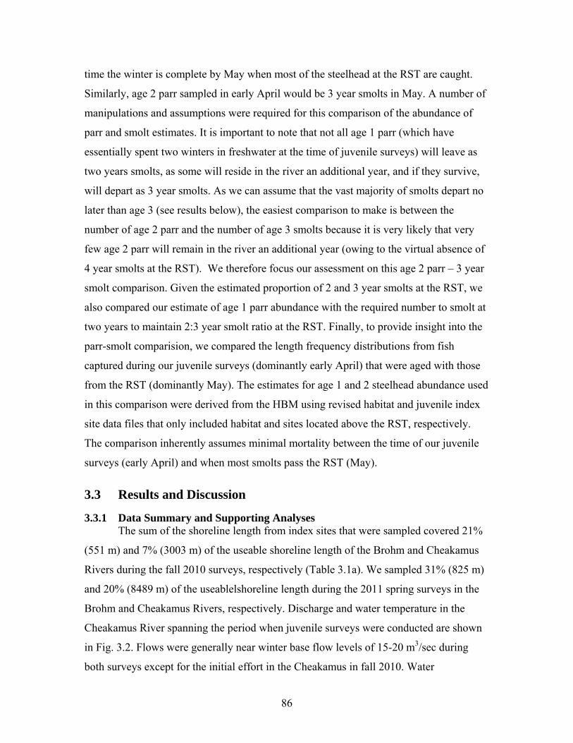
86

time the winter is complete by May when most of the steelhead at the RST are caught.

Similarly, age 2 parr sampled in early April would be 3 year smolts in May. A number of

manipulations and assumptions were required for this comparison of the abundance of

parr and smolt estimates. It is important to note that not all age 1 parr (which have

essentially spent two winters in freshwater at the time of juvenile surveys) will leave as

two years smolts, as some will reside in the river an additional year, and if they survive,

will depart as 3 year smolts. As we can assume that the vast majority of smolts depart no

later than age 3 (see results below), the easiest comparison to make is between the

number of age 2 parr and the number of age 3 smolts because it is very likely that very

few age 2 parr will remain in the river an additional year (owing to the virtual absence of

4 year smolts at the RST). We therefore focus our assessment on this age 2 parr – 3 year

smolt comparison. Given the estimated proportion of 2 and 3 year smolts at the RST, we

also compared our estimate of age 1 parr abundance with the required number to smolt at

two years to maintain 2:3 year smolt ratio at the RST. Finally, to provide insight into the

parr-smolt comparision, we compared the length frequency distributions from fish

captured during our juvenile surveys (dominantly early April) that were aged with those

from the RST (dominantly May). The estimates for age 1 and 2 steelhead abundance used

in this comparison were derived from the HBM using revised habitat and juvenile index

site data files that only included habitat and sites located above the RST, respectively.

The comparison inherently assumes minimal mortality between the time of our juvenile

surveys (early April) and when most smolts pass the RST (May).

3.3 Results and Discussion

3.3.1 Data Summary and Supporting Analyses The sum of the shoreline length from index sites that were sampled covered 21%

(551 m) and 7% (3003 m) of the useable shoreline length of the Brohm and Cheakamus

Rivers during the fall 2010 surveys, respectively (Table 3.1a). We sampled 31% (825 m)

and 20% (8489 m) of the useablelshoreline length during the 2011 spring surveys in the

Brohm and Cheakamus Rivers, respectively. Discharge and water temperature in the

Cheakamus River spanning the period when juvenile surveys were conducted are shown

in Fig. 3.2. Flows were generally near winter base flow levels of 15-20 m3/sec during

both surveys except for the initial effort in the Cheakamus in fall 2010. Water

87

temperature during the fall survey ranged from 9-12 oC in the Cheakamus River and 10-

11 oC in Brohm River. Water temperatures in the Cheakamus and Brohm Rivers during

the spring surveys ranged from 5- 6 oC.

Results from scale ageing (Table 3.4) were used to assign maximum lengths for

age 0, and 1 year old steelhead in Brohm River of 75 and 110 mm in fall 2010, and 75

and 120 mm in spring 2011, respectively. In the Cheakamus River, maximum lengths for

age 0 and 1 year old steelhead in fall 2010 were 80 and 135 mm, and 100 and 130 mm in

spring 2011. We used a maximum length of 180 mm for age 2 steelhead for all strata

which was based on very limited length-at-age data for the upper limit for this age class.

Generally, there has been relatively little variation in size-at-age across years within

rivers in fall (typically ± 5-10 mm). However, there appears to be larger variation in size-

at-age for age 0 fish in the Cheakamus River in the spring sample.

Length frequency distributions (unadjusted for size-dependent detection

probability) for juvenile steelhead based on electrofishing in the fall were dominated by

smaller, mostly age 0 fish (Fig. 3.3 a, c). Length frequency distributions reflect patterns

in abundance among size classes as well as size-specific differences in vulnerability to

sampling gear. Larger and older fish were more prevalent in the spring when snorkeling

was also conducted (Fig. 3.3 b, d). Note that electrofishing and snorkeling were used to

sample Brohm River in spring 2010 and 2011, but only snorkeling was used in 2009.

The absence of a small mode in the spring 2009 Brohm length frequency distribution is

the result of not using electrofishing in this year, which is more efficient at capturing

smaller individuals (Korman et al. 2011).

A total of 1226 and 1535 juvenile steelhead were enumerated at index sites in

Brohm and Cheakamus Rivers in fall 2010, and 449 and 2310 in spring 2011,

respectively (Table 3.5). Catch per effort (CPE) of steelhead was highly variable across

index sites in the Cheakamus River, but sites classified as having “good” habitat quality

for fry and parr had average CPEs that were 2-4 fold higher than sites classified as having

“poor” habitat (Fig. 3.4).

Mark-recapture experiments conducted in fall 2010 and spring 2011 provided

additional data to estimate hyper distributions of detection probability in the HBM (Table

3.6). Aggregating data from all years, detection probability for age-0 steelhead based on

88

electrofishing was relatively consistent among experiments and was almost twice as high

in the Cheakamus River compared to Brohm River (Table 3.7), likely due to the more

porous nature of the substrate in Brohm. For 1+ steelhead, detection probability for

electrofishing was higher in Brohm River than in the Cheakamus River, likely due to

reduced channel width and shallower depths in Brohm. Electrofishing-based detection

probability estimates for age 1+ steelhead in the Cheakamus River were highly uncertain

because few fish are marked due to low capture probability. High variability among sites

for this stratum likely reflects the large uncertainty in detection probability estimates

within sites due to the sampling error induced by low numbers of marked fish. Detection

probability for snorkeling was lower for age 0 steelhead than for 1+ fish due to increased

concealment behavior of smaller fish. Detection probability for age 1+ fish based on

snorkeling was generally high and consistent among sites.

Catch per effort (CPE) in Brohm River in fall was remarkably similar between

2008 and 2010 for all age classes (Table 3.8). Abundance of age 0 steelhead in the spring

sample in 2009 was much lower, likely because electrofishing was not conducted in this

first year. In the Cheakamus River, CPE for age 0 steelhead was approximately two- and

three- fold higher in fall 2008 compared to fall 2009 and 2010, respectively. Catch per

effort for age 1 steelhead in spring 2009 was 4-fold lower than in spring 2010 but similar

to the CPE in 2011.

3.3.3 Estimates of Juvenile Steelhead Abundance from the Hierarchical Bayesian Model An intense and successful sampling effort was implemented in fall 2010 and

spring 2011 in both the Brohm and Cheakamus Rivers, resulting in catch data from a

large number of index sites (Table 3.9). In addition, the multi-year mark-recapture

datasets expanded based on experiments conducted in fall 2010 and spring 2011. These

characteristics led to large improvement in precision (Coefficient of Variation (CV)) of

estimates of juvenile steelhead abundance for the majority of strata, especially for Brohm

River where the number of electrofishing-based mark-recapture experiments doubled

based on fall 2010 and spring 2011 sampling (Table 3.6). An example of output from the

HBM for one strata (Cheakamus River age 1 steelhead in spring 2011) is shown in Figure

3.5. In this example, electrofishing-based detection probability is low, and experiment-

89

specific estimates are uncertain, resulting in considerable shrinkage of HBM-estimated

values compared to the independent estimates (r/R) (Fig. 3.5a and b). Detection

probability for snorkeling is approximately 3-fold higher (Fig. 3.5c and d) and there is

less uncertainty in the estimates because the number of marked fish is greater, resulting in

less shrinkage. Fish densities at index sites were highly variable and generally low (Fig.

3.5e), resulting in a fish density distribution with a long right-hand tail (Fig. 3.5f). Higher

densities of age 1 parr were occasionally seen at sites upstream of Culliton Creek and

between the Cheekye confluence and the Bailey Bridge (3.5e). Due to the large number

of index sites, the total estimate of abundance across the sampled sites was relatively

precise (Fig. 3.5g) even though site-specific densities were highly variable. The majority

of uncertainty in the estimate for the entire river was driven by uncertainty in the estimate

of abundance for the portion of river that was not sampled (Fig. 3.5h), which depends on

uncertainty in the hyper-distribution of fish density (Fig. 3.5f).

Total abundance estimates in fall 2010 and spring 2011 were generally precise

(average CV across 12 strata = 0.16, Table 3.10). Estimates for Brohm River were

slightly more precise than for the Cheakamus owing to sampling a greater proportion of

the river (Table 3.1) and lower variation in densities across sites. Estimates for the

Cheakamus River were generally precise except for age 2 fish in fall 2010, which

resulted from low and variable detection probability coupled with low catch. Note that

abundance estimates for age 1 parr in the Cheakamus River in spring, perhaps the most

important metric we measure as a surrogate for smolt production, had CVs of 0.28, 0.12,

and 0.09 in 2009, 2010, and 2011, respectively. The improving precision is the result of

increasing the number of index sites through time. Note that in spring 2009, the Brohm

age 0 estimate was greater than the age 1 estimate, which was not the case in spring 2010

and 2011. This occurred because both electrofishing and snorkeling were used in the

latter years, but not in 2009. It is very likely that the abundance of age 0 steelhead in

spring 2009 was underestimated due to a positive bias in detection probability for small

fish when snorkeling (Korman et al. 2011). Abundance estimates for Brohm River in fall

2008 were very imprecise, owing to the very limited number of index sites that were

sampled (making it difficult to estimate variation in fish density across sites). Note that

the revised estimates for fall 2008 presented here were based on uninformative priors,

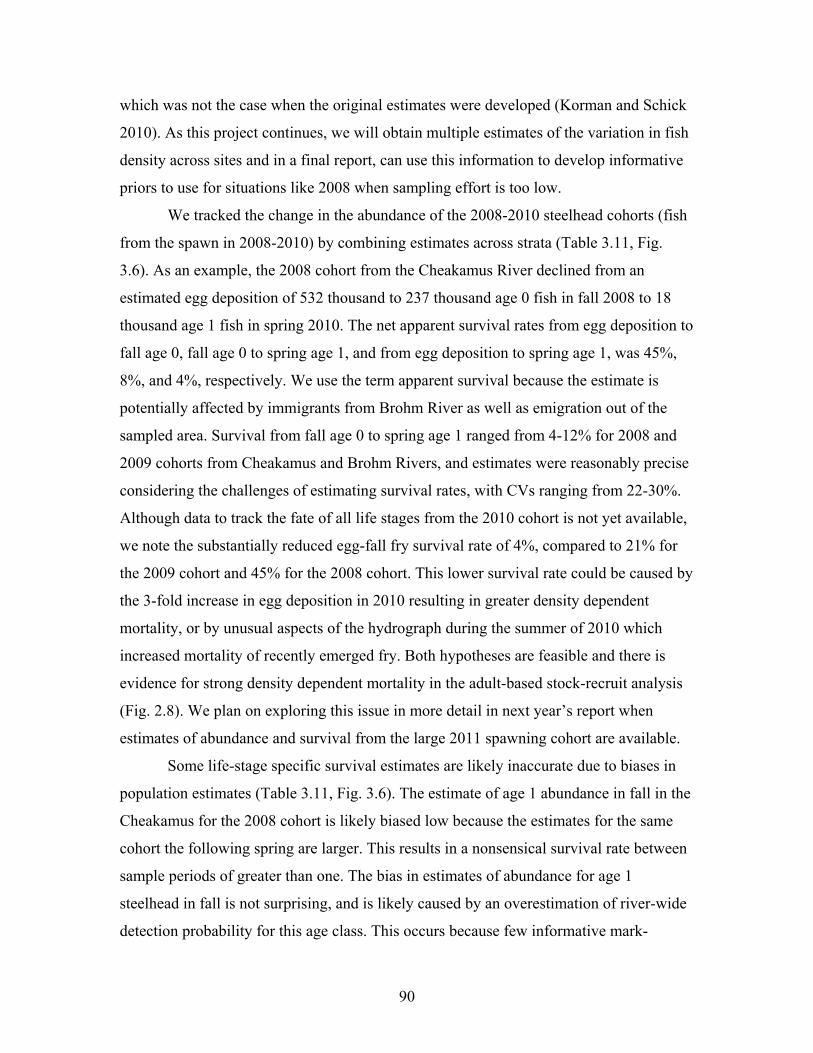
90

which was not the case when the original estimates were developed (Korman and Schick

2010). As this project continues, we will obtain multiple estimates of the variation in fish

density across sites and in a final report, can use this information to develop informative

priors to use for situations like 2008 when sampling effort is too low.

We tracked the change in the abundance of the 2008-2010 steelhead cohorts (fish

from the spawn in 2008-2010) by combining estimates across strata (Table 3.11, Fig.

3.6). As an example, the 2008 cohort from the Cheakamus River declined from an

estimated egg deposition of 532 thousand to 237 thousand age 0 fish in fall 2008 to 18

thousand age 1 fish in spring 2010. The net apparent survival rates from egg deposition to

fall age 0, fall age 0 to spring age 1, and from egg deposition to spring age 1, was 45%,

8%, and 4%, respectively. We use the term apparent survival because the estimate is

potentially affected by immigrants from Brohm River as well as emigration out of the

sampled area. Survival from fall age 0 to spring age 1 ranged from 4-12% for 2008 and

2009 cohorts from Cheakamus and Brohm Rivers, and estimates were reasonably precise

considering the challenges of estimating survival rates, with CVs ranging from 22-30%.

Although data to track the fate of all life stages from the 2010 cohort is not yet available,

we note the substantially reduced egg-fall fry survival rate of 4%, compared to 21% for

the 2009 cohort and 45% for the 2008 cohort. This lower survival rate could be caused by

the 3-fold increase in egg deposition in 2010 resulting in greater density dependent

mortality, or by unusual aspects of the hydrograph during the summer of 2010 which

increased mortality of recently emerged fry. Both hypotheses are feasible and there is

evidence for strong density dependent mortality in the adult-based stock-recruit analysis

(Fig. 2.8). We plan on exploring this issue in more detail in next year’s report when

estimates of abundance and survival from the large 2011 spawning cohort are available.

Some life-stage specific survival estimates are likely inaccurate due to biases in

population estimates (Table 3.11, Fig. 3.6). The estimate of age 1 abundance in fall in the

Cheakamus for the 2008 cohort is likely biased low because the estimates for the same

cohort the following spring are larger. This results in a nonsensical survival rate between

sample periods of greater than one. The bias in estimates of abundance for age 1

steelhead in fall is not surprising, and is likely caused by an overestimation of river-wide

detection probability for this age class. This occurs because few informative mark-

91

recapture experiments for parr in deeper habitats are achieved due to low detection

probability, so the ones from shallow habitats, where detection probability is higher (Fig.

3.7), dominate the estimated hyper distribution and population estimates. For Brohm

River, the age 0 estimate in spring 2009 is very likely biased low (due to snorkeling

only), resulting in a nonsensical survival estimate between spring 2009 and fall 2009. The

survival estimate between fall 2008 and spring 2009 is also likely biased low. Such biases

in Brohm River did not occur after spring 2009 because electrofishing was introduced as

an additional sampling method. The overall fall age-0 to spring age-1 survival rate in

Brohm River is likely unbiased because these two abundance samples are likely unbiased

(electrofishing adequate to sample age 0 fish in fall, and snorkeling and electrofishing

used for age 1 in spring 2010 sample).

Estimates of age 2 parr abundance above the RST in the spring of 2009, 2010, and

2011 were compared to estimates of 3 year smolt abundance at the RST. Juvenile

survey-based estimates were 30% and 19% higher than RST-based ones in 2009 and

2010, respectively, but 30% lower in 2011 (Table 3.12). However, due to the uncertainty

in both types of estimates, these differences could be solely due to sampling error (Fig.

3.8). The required number of age 1 parr to smolt at two years to maintain the 2:3 year

smolt ratio at the RST was well below the estimated age 1 parr abundance in 2010 and

2011. However in 2009, virtually all of the age 1 parr would need to have smolted at two

years, which is unlikely given that 53% of the smolts in 2010 were 3 year olds (i.e., some

age 1 parr must have remained in the Cheakamus in 2009 to eventually smolt as 3 year

olds in 2010). Assuming the 2:3 year smolt ratio and abundance at the RST is correct, this

indicates that age 1 parr abundance in 2009 was likely biased low.

The comparison of juvenile survey- and RST-based abundance estimates depends

entirely on correct and consistent aging of steelhead juveniles from both surveys.

Examination of length frequency distributions for steelhead that were aged indicates there

may be significant discrepancies in the age designations from these two surveys (Table

3.13). These length frequency distributions indicate the age 1 and 2 parr sampled in early

April would need to grow approximately 50-60 mm to match the size distributions of 2

and 3 year smolts at the RST in May. This amount of growth in 1.5-2 months seems

unrealistic and may indicate that fish from the juvenile surveys are over-aged, or fish

92

from the RST survey are under-aged. A reexamination of scales by an independent

biologist will be required to resolve this issue, but our initial suspicion is that smolts at

the RST are under-aged. Ageing of fish from the juvenile survey may be more accurate

because small fish of known age (age 0) are included in the sample and help calibrate age

estimates for older fish. The age 0 fish provide a reference for verifying the presence of

the first winter growth check on fish that can only have one check (i.e. fish < 60 mm in

spring). This check can be difficult to observe owing to the very limited growth from

emergence to the beginning of winter in the first year of life. Observing the first winter

check on fish of known age in spring (age 0) makes it easier to assign correct age classes

to older fish. At the RST, age 0 fish are not aged, so the first winter check may be missed,

resulting in under-aging by one year. The same problem would occur for freshwater ages

assigned from reading of adult scales. It is critical to resolve this ageing discrepancy as it

effects stock-recruit and production analysis for most aspects of the work presented here.

Further, until it is resolved, the comparison of juvenile survey- and RST-based abundance

estimates should be considered highly preliminary. If the ageing discrepancy is

substantive, the current evaluation (Table 3.12 and Fig. 3.8) is an apples-to-oranges

comparison.

3.4 Conclusions Juvenile steelhead population estimates in the Cheakamus and Brohm Rivers are

generally quite precise due to increases in the number of index sites and the accumulation

of mark-recapture data across years. The former provided better information on mean fish

densities and variation in fish densities across sites, while the latter provided additional

data on detection probability. In the Cheakamus River, most population estimates had

CVs that were less than 0.2. At the currently level of effort, estimates for age 1 parr in the

spring, which may be our best proxy of potential smolt production, are very precise (CV

~0.1). Estimates of steelhead smolt production derived from juvenile surveys in spring

2008-2011 were within 30% of estimates from the Rotary Screw Trap. This indicates that

production estimates from the juvenile survey are likely relatively unbiased. However,

this evaluation is a relatively insensitive test when one considers the uncertainty in both

juvenile survey- and RST-based estimates. Further, this comparison should be considered

93

highly preliminary until ageing discrepancies between fish collected during juvenile and

RST surveys are resolved.

The most significant finding from the analysis is the demonstration that it is

possible to estimate survival rates of juvenile steelhead after 2 winters in freshwater.

Survival from age 0 in the fall to age 1 in the spring (i.e., 2 winters in freshwater) was 4-

8% and 5-12% in the Cheakamus and Brohm Rivers, respectively with CVs between 0.22

and 0.3. This precision will likely allow evaluation of the effects of major changes in

flow and other abiotic and biotic factors on juvenile survival rates. Given reasonably

accurate escapement estimates and information on the size of returning spawners, it is

also be possible to compute egg-fry and egg-parr survival rates. Estimates of egg-fall fry

survival in the Cheakamus River were 45%, 21%, and 4% for 2008, 2009, and 2010

spawning cohorts. Such estimates can be compared over time and to literature values in

unregulated streams to evaluate potential effects of the current and future flow regimes.

The substantive decrease in egg-fall fry survival in 2010 may be due to the much greater

egg deposition in that year, resulting in greater density dependent mortality.

Alternatively, rapid stage reductions in summer of 2010 when fry were utilizing

vulnerable low angle cobble bars may have increased the overall summer mortality rate.

We should be able to resolve this uncertainty based on data from 2011 where egg

deposition was high and when these rapid drawdowns did not occur. If egg-fall fry

survival rates for the 2011 cohort are similar to 2008 and 2009, this would indicate that

rapid drawdowns are having a substantive effect on production.

In spring 2010, fall 2010, and spring 2011 samples, catch per effort was two- to

four-fold higher in sites classified as having good rather than poor quality habitat for age

0 and 1+ steelhead. However, there was considerable variation in catch per effort across

sites classified as either poor or good quality habitat. Clearly, other habitat attributes and

non-habitat effects (proximity to spawning locations, predator concentrations, food

availability, water quality) are having an important effect on local juvenile steelhead

abundance in this system. In a future analysis, we will use simulation techniques to

evaluate the potential gains in precision that can be achieved through a habitat quality-

stratified sampling design. The effectiveness of such a stratified depends on both the

94

differences in mean density across habitat quality classes as well as the variation in

density within classes.

3.5 References Berger, A.M. and R.E. Gresswell. 2009. Factors influence coastal cutthroat trout seasonal

survival rates: a spatially continuous approach within stream networks. Can. J.

Fish. Aquat. Sci 66: 613-632.

Bohlin, T. 1978. Temporal changes in the spatial distribution of juvenile sea-trout Salmo

trutta in a small stream. Oikos 30: 114-120.

Bradford, M.J., Taylor, G.C., Allan, J.A., and P.S. Higgins. 1995. An experimental study

of the stranding of juvenile coho salmon and rainbow trout during rapid flow

decreases under winter fluctuations. Nor. Am. J. Fish. Manage. 15:473-479.

Contor, G.R., and J.S. Griffith. 1995. Nocturnal emergence of juvenile rainbow trout

from winter concealment relative to light intensity. Hydrobiologia 299:179-183.

Elliott, J.M. 1994. Quantitative ecology and the brown trout. Oxford University Press,

Oxford. 286 p.

Gelman, A. 2006. Prior distributions for variance parameters in hierarchical models.

Bayesian Analysis 1:515-533.

Gibson, A.J.F., Bowlby, H.D. and P.G. Amiro. 2008. Are wild populations ideally

distributed? Variations in density-dependent habitat use by age class in juvenile

Atlantic salmon. Can. J. Fish. Aquat. Sci. 65: 1667-1680.

Girard, I.L., Grand, J.W.A., and S.O. Steingrimsson. 2004. Foraging, growth, and loss

rate of young-of-the-year Atlantic salmon (Salmo salar) in relation to habitat use

in Catamaran Brook, New Brunswick. Canadian Journal of Fisheries and Aquatic

Sciences 61: 2339-2349.

Harvey, B.C., White, J.L. and R.J. Nakamoto. 2005. Habitat-specific biomass, survival,

and growth of rainbow trout during summer in a small coastal stream. Can. J.

Fish. Aquat. Sci. 62: 650-658.

Hvidsten, N.A. 1993. High winter discharge after regulation increases production of

Atlantic salmon smolts in the River Orkla, Norway. In Production of juvenile

Atlantic salmon, Salmo salar, in natural waters. R.J. Gibson and R.E. Cutting

[eds.]. Can. Sp. Pub. Fish. Aquat. Sci 118.

95

He, Y. and J.S. Hodges. 2008. Point estimates for variance-structure parameters in

Bayesian analysis of hierarchical models. Comp. Stat. Data Anal. 52: 2560 -

2577.

Jensen, A.J., and B.O. Johnsen. 1999. The functional relationship between peak spring

floods and survival and growth of juvenile Atlantic salmon (Salmo salar) and

brown trout (Salmo trutta). Funct. Ecol. 13: 778-785.

Korman, J., Schick, J., Melville, C, and D. McCubbing. 2011. Cheakamus River

steelhead juvenile and adult abundance monitoring, Fall 2009 to Spring 2010

(Year 4). Report prepared for BC Hydro by Ecometric Research, August 2011.

http://www.bchydro.com/planning_regulatory/water_use_planning/lower_mainla

nd.html#Cheakamus

Korman, J., Schick, J., and A. Clarke. 2010. Cheakamus River steelhead juvenile and

adult abundance monitoring Fall 2008 – Spring 2009. Report prepared for BC

Hydro by Ecometric Research, February 2010.

http://www.bchydro.com/planning_regulatory/water_use_planning/lower_mainla

nd.html#Cheakamus

Korman, J., Decker, A.S., Mossop, B., and J. Hagen. 2010. Comparison of electrofishing-

and snorkeling mark-recapture estimation of juvenile steelhead in a medium-sized

river. North American Journal of Fisheries Management 30: 1280-1302.

Korman, J. 2008. Cheakamus river steelhead adult abundance, and juvenile habitat use

and abundance monitoring, 2007-2008, final report. Report prepared for BC

Hydro by Ecometric Research, September 29, 2009. 99 pp.

Marmorek, D.R. and I. Parnell. 2002. Cheakamus River water use plan. Report of the

consultative committee. Report prepared on behalf of the Cheakamus River Water

Use Plan Consultative Committee by Essa Technologies Ltd.

96

Melville, C.C. and D.J. McCubbing. 2011. Cheakamus River – Juvenile salmonid

outmigration enumeration assessment spring 2011. Report prepared by Instream

Fisheries Research Inc. for BC Hydro.

Melville, C.C. and D.J. McCubbing. 2010. Cheakamus River – Juvenile salmonid

outmigration enumeration assessment spring 2010. Report prepared by Instream

Fisheries Research Inc. for BC Hydro.

Melville, C.C. and D.J. McCubbing. 2009. Cheakamus River – Juvenile salmonid

outmigration enumeration assessment spring 2009. Report prepared by Instream

Fisheries Research Inc. for BC Hydro.

Mitro, M.G., Zale, A.V., and B.A. Rich. 2003. The relation between age-0 rainbow trout

abundance and winter discharge in a regulated river. Can. J. Fish. Aquat. Sci. 60:

135 –139.

Nislow, K.H. Einum, S., and C.L. Folt. 2004. Testing predictions of the critical period for

survival concept using experiments with stocked Atlantic salmon. Journal of Fish

Biology. 65 (Supplement A): 188 - 200.

R Development Core Team. 2009. R: A Language and Environment for Statistical

Computing. Vienna, Austria: R Foundation for Statistical Computing. Available

at: http://www.R-project.org.

Rosenfeld, J.S., and S. Boss. 2001. Fitness consequences of habitat use for juvenile

cutthroat trout: energetic costs and benefits in pools and riffles. Canadian Journal

of Fisheries and Aquatic Sciences 58: 585-593.

Rosenfeld, J.S., Leiter, T., Lindner, G., and L. Rothman. 2005. Food abundance and fish

density alters habitat selection, growth, and habitat suitability curves for juvenile

coho salmon. Can. J. Fish. Aquat. Sci 62: 1691-1701.

Saltveit, S.J., Halleraker, J.H., Arnekleiv, J.V., and A. Harby. 2001. Field experiments on

stranding in juvenile Atlantic Salmon (Salmo Salar) and Brown Trout (Salmo

Trutta) during rapid flow decreases caused by hydropeaking. Regulated Rivers

17: 609-622.

Spiegelhalter, D.J., Thomas A., Best, N.G., and Lunn, D. 1999. WinBUGS User Manual:

Version 1.4. Cambridge: MRC Biostatistics Unit, 60 pp.

97

Sturtz, S., Legges U., and Gelman A. 2005. R2WinBGS: a package for running

WinBUGS from R. Journal of statistical software 3: 1-16.

Van Dischoeck, P. 2000. Squamish River system juvenile steelhead sampling program.

Report prepared for BC Ministry of Environment, Lands, and Parks by Aquatic

Resources Limited.

Wyatt, R.J. 2003. Mapping the abundance of riverine fish populations: integrating

hierarchical Bayesian models with a geographic information system (GIS). Can. J.

Fish. Aquat. Sci. 60: 997-1007.

Wyatt, R.J. 2002. Estimating riverine fish population size from single- and multiple-pass

removal sampling using a hierarchical model. Can. J. Fish. Aquat. Sci 59: 695-

706.

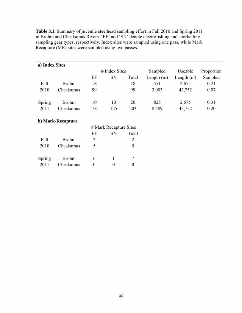
98

Table 3.1. Summary of juvenile steelhead sampling effort in Fall 2010 and Spring 2011 in Brohm and Cheakamus Rivers. ‘EF’ and ‘SN’ denote electrofishing and snorkelling sampling gear types, respectively. Index sites were sampled using one pass, while Mark Recapture (MR) sites were sampled using two passes. a) Index Sites

# Index Sites Sampled Useable ProportionEF SN Total Length (m) Length (m) Sampled

Fall Brohm 18 18 551 2,675 0.21 2010 Cheakamus 99 99 3,003 42,752 0.07

Spring Brohm 10 10 20 825 2,675 0.31 2011 Cheakamus 78 125 203 8,489 42,752 0.20

b) Mark-Recapture # Mark Recapture Sites EF SN Total

Fall Brohm 2 2 2010 Cheakamus 5 5

Spring Brohm 6 1 7 2011 Cheakamus 0 0 0

99

Table 3.2. Definition of variables of the hierarchical Bayesian model used to estimate juvenile steelhead abundance in the Cheakamus and Brohm Rivers.

Variable Description

Data ri.g Marks detected at mark-recapture site i for gear type gmi,g Marks released at mark-recapture site i for gear type gcj,g Fish detected at index site j for gear type glj Shoreline length for index site jhr Total shoreline length in reach r

Site-Specific Parameters i,g Estimated detection probability at mark-recapture site i for gear type gj,g Simulated detection probability for index site j for gear type g j Estimated density (fish/m) at index site j

Hyper-Parameters ,g Mean of beta hyper-distribution for detection probability for gear type g,g Precision of beta hyper-distribution for detection probability for gear type g Mean of normal hyper-distribution for log fish density Precision of normal hyper-distribution for log fish density

Derived Variables i,g Parameter for beta hyper distribution of detection probability i,g Parameter for beta hyper distribution of detection probability Nj,g Abundance at index site j sampled by gear type gNsr Total abundance across all index sites in reach rNusr Total abundance in unsampled shoreline in reach rNtr Total abundance in reach rNt Total abundance across all reaches

Indices and Constants i Index for mark-recapture sitej Index for single-pass index site g Index for gear type (SN or EF)r Index for reach

100

Table 3.3. Equations of the hierarchical Bayesian model used to estimate juvenile steelhead abundance in the Brohm and Cheakamus Rivers. See Table 3.2 for definition of model parameters, constants, and subscripts. Lower case Arabic letters denote data or indices (if subscripts). Capital Arabic letters denoted derived variables, which are computed as a function of estimated parameters. Greek letters denote estimated parameters. Parameters with Greek letter subscripts are hyper-parameters. Detection Model (3.1) ),(~ ,,, gigigi mdbinr

(3.2) ),(~, gggi dbeta

Population Model (3.3) ),(~, gggj dbeta

(3.4) ),(~ ,,, gjgjgj Ndbinc

(3.5) )(~, jjgj ldpoisN

(3.6) ),(~)log( dnormj

(3.7)

g rj

gjr nNs ,

(3.8) )](5.0exp[ 1

rj

jrr lhNus

(3.9) rrr NusNsNt (3.10)

rrNtNt

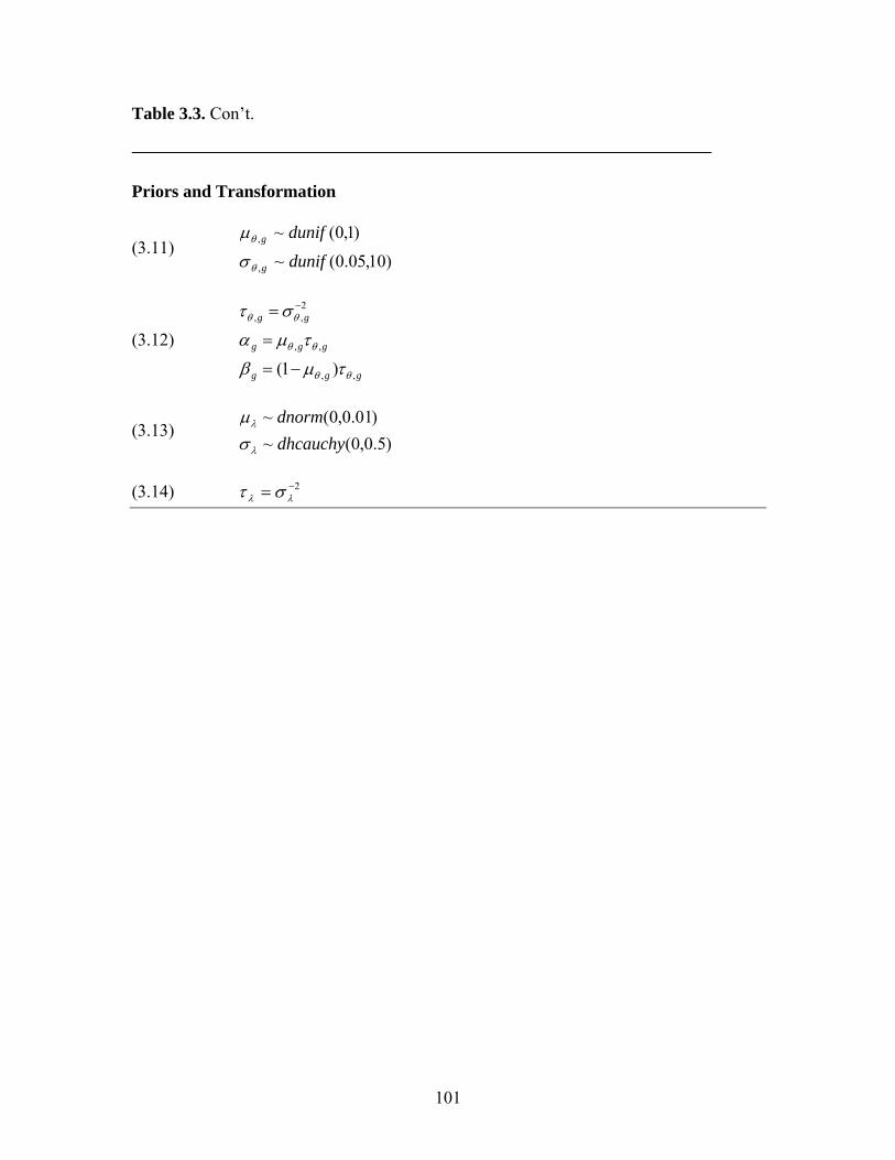
101

Table 3.3. Con’t.

Priors and Transformation

(3.11) )10,05.0(~

)1,0(~

,

,

dunif

dunif

g

g

(3.12)

ggg

ggg

gg

,,

,,

2,,

)1(

(3.13) )5.0,0(~

)01.0,0(~

dhcauchy

dnorm

(3.14) 2

102

Table 3.4. Number of juvenile steelhead captured in Brohm and Cheakamus Rivers assigned to each age-class by 5 mm fork length bin determined from scales in fall (a) and spring (b). Yellow-shaded cells indicate the maximum size cut-offs used to assign ages based on fork length for fish that were not aged. a) Fall

ForkLength(mm) 0 1 2 0 1 2 0 1 2 0 1 2 0 1 2 0 1 2<45 2

45-49 6 150-54 8 1 455-59 3 6 860-64 1 6 1065-69 2 1 1 11 370-74 1 1 3 1 1 6 1 375-79 2 2 1 3 3 2 6 180-84 1 3 4 1 4 2 1 285-89 2 6 2 190-94 4 4 5 3 595-99 3 4 3 5 2

100-104 1 4 3 3 3 3105-109 4 3 1 7 4 2110-114 2 1 6 1 4115-119 1 2 4 1 2120-124 1 1 2 6 1 3 2125-129 1 2 2 4 5 1 2 1130-134 1 3 6 2 2 3 3135-139 1 2 1 1 1140-144 1 1 3 2 4145-149 1 2 2150-154 1 1155-159 1 2160-164 3 1170-174 1 2175-179 2 1185-190 1

>190 1Total 2 11 4 28 10 24 28 13 2 32 16 38 45 9 35 19 17

Brohm Cheakamus2008 2009 2010 2008 2009 2010

103

Table 3.4. Con’t. b) Spring

Fork

Length(mm) 0 1 2 0 1 2 0 1 2 0 1 2 0 1 2 0 1 2 0 1 2<45 1

45-49 5 1 150-54 2 4 5 2 355-59 1 1 4 3 6 460-64 9 4 6 3 1 765-69 4 2 2 6 1 670-74 1 3 1 6 6 2 675-79 1 1 3 6 4 7 180-84 2 1 1 1 6 1 1 5 6 185-89 3 1 1 6 1 3 2 11 5 190-94 2 2 6 7 7 2 10 6 195-99 4 2 4 3 1 2 1 11 5 3

100-104 3 3 1 1 1 7 1 4105-109 1 4 6 1 3 12 2 6110-114 1 1 1 2 5 6115-119 1 5 1 6 5 4 1120-124 2 2 8 1 4 1 5 3125-129 3 1 1 7 1 1 1 2 1130-134 4 3 4 1 2 2135-139 1 7 3 1 7 2 1 3 2140-144 6 4 1 2 1 2 2145-149 2 3 3 4 1 1 4 1150-154 1 1 1 2 1 2 4155-159 1 1 2 4 3 4160-164 1 2 1 1 1 1165-169 1 1 1 1 1 5170-174 1175-179 1 1 1180-184 2 1185-190 1

Total 2 16 6 20 19 1 21 34 37 1 29 15 43 38 15 33 81 17 60 39 24

2011Brohm Cheakamus

2009 2010 2011 2008 2009 2010

104

Table 3.5. Total number of juvenile steelhead captured by electrofishing (EF) or observed by snorkelling (SN) summed across all index sites in Brohm and Cheakamus Rivers by age class.

Season Gear River Age Year 0+ 1+ 2+ 0+ - 2+

Fall EF Brohm 827 212 187 1,226 2010 EF Cheakamus 1,451 59 25 1,535

Spring EF Brohm 103 58 28 189 2011 SN 25 91 144 260

EF Cheakamus 696 27 16 739 SN 1,063 304 204 1,571

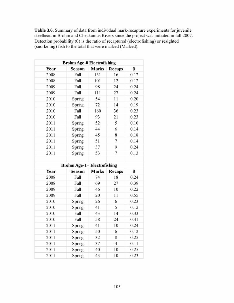
105

Table 3.6. Summary of data from individual mark-recapture experiments for juvenile steelhead in Brohm and Cheakamus Rivers since the project was initiated in fall 2007. Detection probability () is the ratio of recaptured (electrofishing) or resighted (snorkeling) fish to the total that were marked (Marked).

Year Season Marks Recaps 2008 Fall 131 16 0.122008 Fall 101 12 0.122009 Fall 98 24 0.242009 Fall 111 27 0.242010 Spring 54 11 0.202010 Spring 72 14 0.192010 Fall 160 36 0.232010 Fall 93 21 0.232011 Spring 52 5 0.102011 Spring 44 6 0.142011 Spring 45 8 0.182011 Spring 51 7 0.142011 Spring 37 9 0.242011 Spring 53 7 0.13

Year Season Marks Recaps 2008 Fall 74 18 0.242008 Fall 69 27 0.392009 Fall 46 10 0.222009 Fall 20 11 0.552010 Spring 26 6 0.232010 Spring 41 5 0.122010 Fall 43 14 0.332010 Fall 58 24 0.412011 Spring 41 10 0.242011 Spring 50 6 0.122011 Spring 32 8 0.252011 Spring 37 4 0.112011 Spring 40 10 0.252011 Spring 43 10 0.23

Brohm Age-1+ Electrofishing

Brohm Age-0 Electrofishing

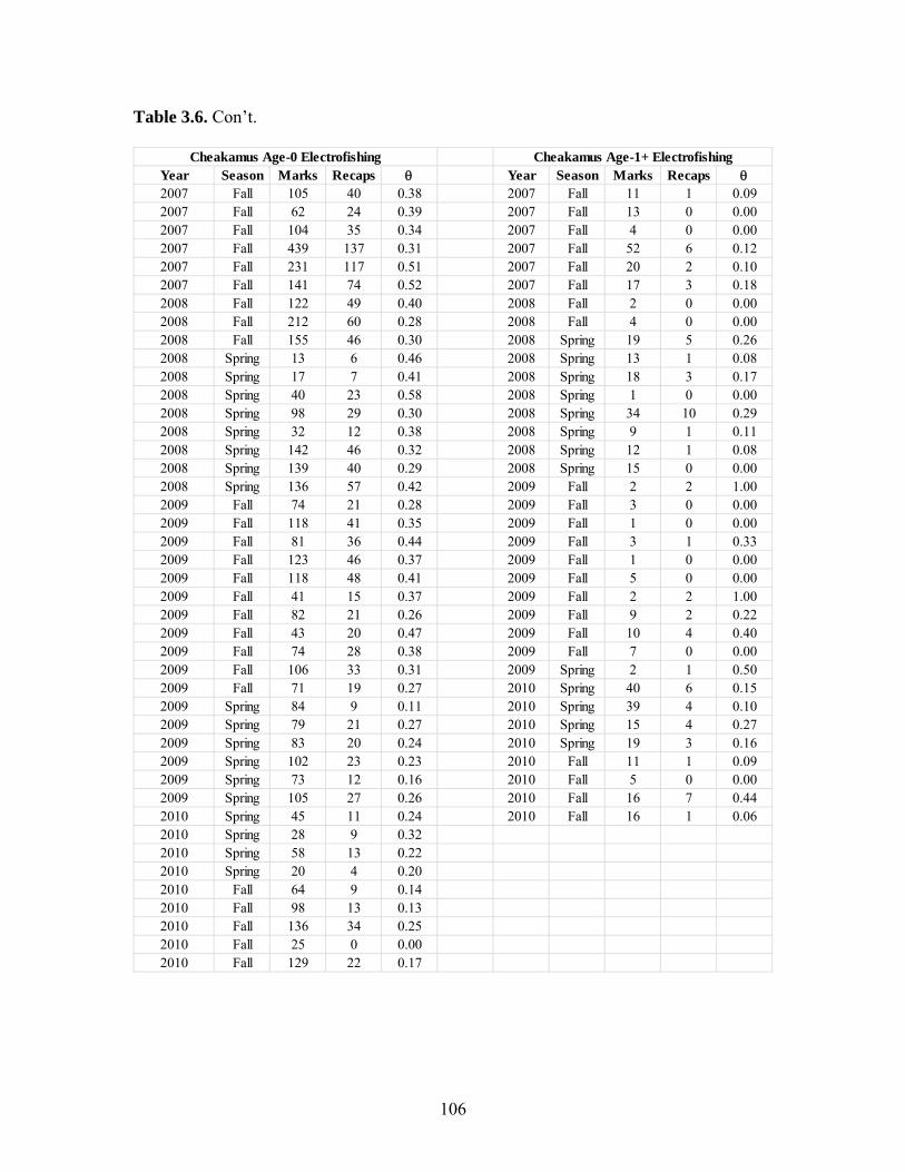
106

Table 3.6. Con’t.

Year Season Marks Recaps Year Season Marks Recaps 2007 Fall 105 40 0.38 2007 Fall 11 1 0.092007 Fall 62 24 0.39 2007 Fall 13 0 0.002007 Fall 104 35 0.34 2007 Fall 4 0 0.002007 Fall 439 137 0.31 2007 Fall 52 6 0.122007 Fall 231 117 0.51 2007 Fall 20 2 0.102007 Fall 141 74 0.52 2007 Fall 17 3 0.182008 Fall 122 49 0.40 2008 Fall 2 0 0.002008 Fall 212 60 0.28 2008 Fall 4 0 0.002008 Fall 155 46 0.30 2008 Spring 19 5 0.262008 Spring 13 6 0.46 2008 Spring 13 1 0.082008 Spring 17 7 0.41 2008 Spring 18 3 0.172008 Spring 40 23 0.58 2008 Spring 1 0 0.002008 Spring 98 29 0.30 2008 Spring 34 10 0.292008 Spring 32 12 0.38 2008 Spring 9 1 0.112008 Spring 142 46 0.32 2008 Spring 12 1 0.082008 Spring 139 40 0.29 2008 Spring 15 0 0.002008 Spring 136 57 0.42 2009 Fall 2 2 1.002009 Fall 74 21 0.28 2009 Fall 3 0 0.002009 Fall 118 41 0.35 2009 Fall 1 0 0.002009 Fall 81 36 0.44 2009 Fall 3 1 0.332009 Fall 123 46 0.37 2009 Fall 1 0 0.002009 Fall 118 48 0.41 2009 Fall 5 0 0.002009 Fall 41 15 0.37 2009 Fall 2 2 1.002009 Fall 82 21 0.26 2009 Fall 9 2 0.222009 Fall 43 20 0.47 2009 Fall 10 4 0.402009 Fall 74 28 0.38 2009 Fall 7 0 0.002009 Fall 106 33 0.31 2009 Spring 2 1 0.502009 Fall 71 19 0.27 2010 Spring 40 6 0.152009 Spring 84 9 0.11 2010 Spring 39 4 0.102009 Spring 79 21 0.27 2010 Spring 15 4 0.272009 Spring 83 20 0.24 2010 Spring 19 3 0.162009 Spring 102 23 0.23 2010 Fall 11 1 0.092009 Spring 73 12 0.16 2010 Fall 5 0 0.002009 Spring 105 27 0.26 2010 Fall 16 7 0.442010 Spring 45 11 0.24 2010 Fall 16 1 0.062010 Spring 28 9 0.322010 Spring 58 13 0.222010 Spring 20 4 0.202010 Fall 64 9 0.142010 Fall 98 13 0.132010 Fall 136 34 0.252010 Fall 25 0 0.002010 Fall 129 22 0.17

Cheakamus Age-0 Electrofishing Cheakamus Age-1+ Electrofishing

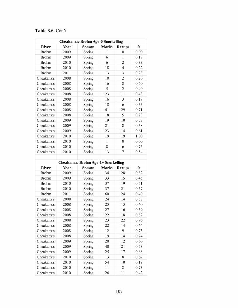
107

Table 3.6. Con’t.

River Year Season Marks Recaps Brohm 2009 Spring 1 0 0.00Brohm 2009 Spring 6 1 0.17Brohm 2010 Spring 6 2 0.33Brohm 2010 Spring 18 4 0.22Brohm 2011 Spring 13 3 0.23

Cheakamus 2008 Spring 10 2 0.20Cheakamus 2008 Spring 16 8 0.50Cheakamus 2008 Spring 5 2 0.40Cheakamus 2008 Spring 23 11 0.48Cheakamus 2008 Spring 16 3 0.19Cheakamus 2008 Spring 18 6 0.33Cheakamus 2008 Spring 41 29 0.71Cheakamus 2008 Spring 18 5 0.28Cheakamus 2009 Spring 19 10 0.53Cheakamus 2009 Spring 21 8 0.38Cheakamus 2009 Spring 23 14 0.61Cheakamus 2010 Spring 19 19 1.00Cheakamus 2010 Spring 1 0 0.00Cheakamus 2010 Spring 8 6 0.75Cheakamus 2010 Spring 13 7 0.54

River Year Season Marks Recaps Brohm 2009 Spring 34 28 0.82Brohm 2009 Spring 33 15 0.45Brohm 2010 Spring 37 19 0.51Brohm 2010 Spring 37 21 0.57Brohm 2011 Spring 60 24 0.40

Cheakamus 2008 Spring 24 14 0.58Cheakamus 2008 Spring 25 15 0.60Cheakamus 2008 Spring 27 16 0.59Cheakamus 2008 Spring 22 18 0.82Cheakamus 2008 Spring 23 22 0.96Cheakamus 2008 Spring 22 14 0.64Cheakamus 2008 Spring 12 9 0.75Cheakamus 2008 Spring 19 14 0.74Cheakamus 2009 Spring 20 12 0.60Cheakamus 2009 Spring 40 21 0.53Cheakamus 2009 Spring 25 17 0.68Cheakamus 2010 Spring 13 8 0.62Cheakamus 2010 Spring 54 10 0.19Cheakamus 2010 Spring 11 8 0.73Cheakamus 2010 Spring 26 11 0.42

Cheakamus-Brohm Age-0 Snorkelling

Cheakamus-Brohm Age-1+ Snorkelling

108

Table 3.7. Summary statistics of detection probability from mark-recapture experiemtns in Brohm and Cheakamus Rivers since the project was initiated in fall 2007 based on electrofishing (EF) and snorkeling (SN). ‘N’, ‘Mean’, and ‘CV’ denote the sample size (# of experiments), mean detection probability, and coefficient of variation in detection probability across experiments within each strata.

Strata N Mean CV

Brohm Age-0 EF 14 0.18 0.30 Brohm Age-1+ EF 14 0.26 0.46 Cheakamus Age-0 EF 43 0.31 0.38 Cheakamus Age-1+ EF 35 0.18 1.39 Both Rivers, Age-0 SN 20 0.39 0.64 Both Rivers, Age-1+ SN 20 0.61 0.28

Table 3.8. Comparison of juvenile steelhead catch per effort (fish per km sampled) across years and seasons where random sampling has been implemented.

Age River Season Year 0 1 2

Brohm Fall 2008 1,488 512 291 2009 1,646 510 249 2010 1,501 385 339

Spring 2009 73 590 125 2010 283 595 203 2011 155 181 208

Cheakamus Fall 2008 1,550 85 32 2009 606 36 9 2010 483 20 8

Spring 2009 225 42 16 2010 124 183 41 2011 207 39 26

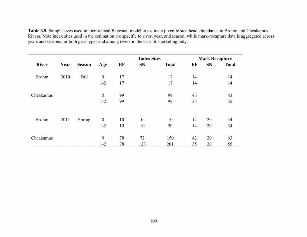
109

Table 3.9. Sample sizes used in hierarchical Bayesian model to estimate juvenile steelhead abundance in Brohm and Cheakamus Rivers. Note index sites used in the estimation are specific to river, year, and season, while mark-recapture data is aggregated across years and seasons for both gear types and among rivers in the case of snorkeling only.

Index Sites Mark Recapture River Year Season Age EF SN Total EF SN Total

Brohm 2010 Fall 0 17 17 14 14 1-2 17 17 14 14

Cheakamus 0 99 99 43 43 1-2 99 99 35 35

Brohm 2011 Spring 0 10 0 10 14 20 34 1-2 10 10 20 14 20 34

Cheakamus 0 78 72 150 43 20 63 1-2 78 123 201 35 20 55

110

Table 3.10. Statistics of total population estimates (in thousands) for juvenile steelhead in the Brohm and Cheakamus Rivers. CV denotes coefficient of variation, while LCL and UCL denote the lower and upper bound of the 95% credible interval, respectively. All estimates were based on uninformative prior distributions.

River Year Season Age Mean Median CV LCL UCL

Cheakamus 2008 Fall 0 246.2 237.5 0.21 169.5 369.2 1 26.7 24.7 0.36 15.1 49.8 2 13.2 9.4 1.4 4.2 45.9

2009 Spring 0 50.9 48.8 0.23 33.7 79.8 1 6.5 6.2 0.28 4.2 10.8 2 2.4 2.2 0.32 1.4 4.2

Brohm 2008 Fall 0 26.0 22.9 0.68 14.5 53.5 1 8.3 5.5 9.5 3.4 13.8 2 Did not converge due to low density/sample size

2009 Spring 0 0.5 0.5 0.9 0.3 0.9 1 2.8 2.7 0.2 2.0 3.9 2 0.6 0.6 0.23 0.4 0.9

Cheakamus 2009 Fall 0 101.1 97.4 0.22 68.9 157.3 1 12.1 10.8 0.45 6.6 25.3 2 2.7 2.4 0.51 1.2 6.2

2010 Spring 0 24.3 23.3 0.22 16.5 37.5 1 18.7 18.4 0.12 15.1 23.7 2 3.8 3.7 0.23 2.6 6.0

Brohm 2009 Fall 0 25.0 24.1 0.21 17.9 37.3 1 5.4 5.3 0.15 4.1 7.2 2 2.6 2.5 0.2 1.8 3.9

2010 Spring 0 5.2 5.0 0.31 3.4 8.7 1 2.8 2.8 0.1 2.3 3.3 2 1.1 1.0 0.17 0.8 1.4

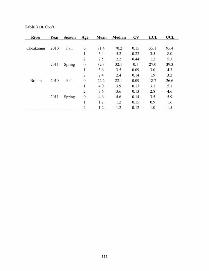
111

Table 3.10. Con’t.

River Year Season Age Mean Median CV LCL UCL

Cheakamus 2010 Fall 0 71.4 70.2 0.15 55.1 95.4 1 5.4 5.2 0.22 3.5 8.0 2 2.5 2.2 0.44 1.2 5.3

2011 Spring 0 32.3 32.1 0.1 27.0 39.3 1 3.6 3.5 0.09 3.0 4.3 2 2.4 2.4 0.14 1.9 3.2

Brohm 2010 Fall 0 22.2 22.1 0.09 18.7 26.6 1 4.0 3.9 0.13 3.1 5.1 2 3.6 3.6 0.13 2.8 4.6

2011 Spring 0 4.6 4.6 0.14 3.5 5.9 1 1.2 1.2 0.15 0.9 1.6 2 1.2 1.2 0.12 1.0 1.5

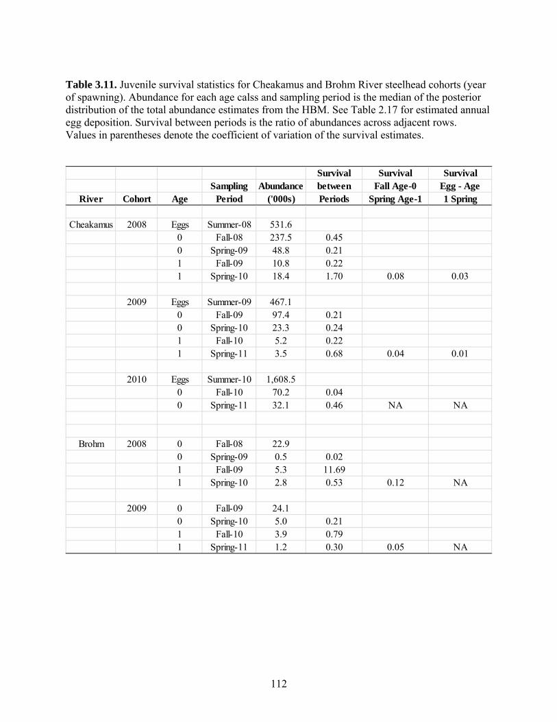
112

Table 3.11. Juvenile survival statistics for Cheakamus and Brohm River steelhead cohorts (year of spawning). Abundance for each age calss and sampling period is the median of the posterior distribution of the total abundance estimates from the HBM. See Table 2.17 for estimated annual egg deposition. Survival between periods is the ratio of abundances across adjacent rows. Values in parentheses denote the coefficient of variation of the survival estimates.

Survival Survival SurvivalSampling Abundance between Fall Age-0 Egg - Age

River Cohort Age Period ('000s) Periods Spring Age-1 1 Spring

Cheakamus 2008 Eggs Summer-08 531.60 Fall-08 237.5 0.450 Spring-09 48.8 0.211 Fall-09 10.8 0.221 Spring-10 18.4 1.70 0.08 0.03

2009 Eggs Summer-09 467.10 Fall-09 97.4 0.210 Spring-10 23.3 0.241 Fall-10 5.2 0.221 Spring-11 3.5 0.68 0.04 0.01

2010 Eggs Summer-10 1,608.50 Fall-10 70.2 0.040 Spring-11 32.1 0.46 NA NA

Brohm 2008 0 Fall-08 22.90 Spring-09 0.5 0.021 Fall-09 5.3 11.691 Spring-10 2.8 0.53 0.12 NA

2009 0 Fall-09 24.10 Spring-10 5.0 0.211 Fall-10 3.9 0.791 Spring-11 1.2 0.30 0.05 NA

113

Table 3.12. Comparison of steelhead smolt production estimates for the Cheakamus River from 2009-2011 based on the Rotary Screw Trap program (Melville and McCubbing, 2011) with those derived from juvenile surveys. Juvenile parr abundance estimates are the medians of the posterior distributions from the HBM. The age 1 parr – 2 yr smolt proportion are estimates of the proportion of age 1 parr (2 winters in freshwater) that will outmigrate as 2 yr smolts. Estimates of smolt numbers from the RST exclude side channel production and are based on a Pooled Peterson estimate. Shaded cells show the key comparison (age 2 parr vs. 3 Yr smolts).

2009 2010 2011 Juvenile Survey Parr Abundance Age 1 Parr (--> 2 Yr Smolt) 5,130 13,990 2400 Age 2 Parr (--> 3 Yr Smolt) 1,580 2,810 1580

RST Estimates of Smolts 5,314 4,494 3812 % 2 Yr Smolts 77% 47% 38% 2:3 Yr Smolt Ratio 3.36 0.90 0.62 2 Yr Smolts 4,096 2,129 1,458 3 Yr Smolts 1,218 2,365 2,354

RST 3 Yr Smolt / Juvenile Survey Age 2 Parr 0.77 0.84 1.49

Age 1 Parr to maintain 2:3 Yr smolt ratio 5,315 2,529 978 Proportion Age 1 Parr Smolting at 2 Yr 1.04 0.18 0.41

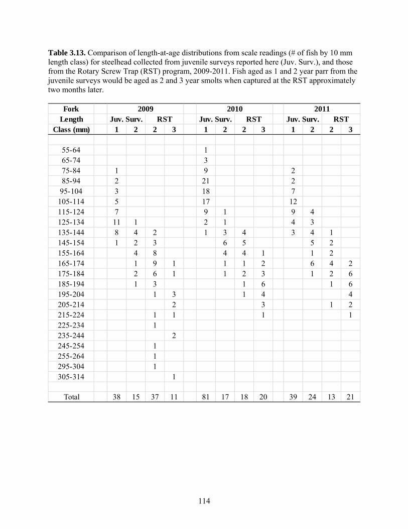
114

Table 3.13. Comparison of length-at-age distributions from scale readings (# of fish by 10 mm length class) for steelhead collected from juvenile surveys reported here (Juv. Surv.), and those from the Rotary Screw Trap (RST) program, 2009-2011. Fish aged as 1 and 2 year parr from the juvenile surveys would be aged as 2 and 3 year smolts when captured at the RST approximately two months later.

ForkLength

Class (mm) 1 2 2 3 1 2 2 3 1 2 2 3

55-64 165-74 375-84 1 9 285-94 2 21 295-104 3 18 7105-114 5 17 12115-124 7 9 1 9 4125-134 11 1 2 1 4 3135-144 8 4 2 1 3 4 3 4 1145-154 1 2 3 6 5 5 2155-164 4 8 4 4 1 1 2165-174 1 9 1 1 1 2 6 4 2175-184 2 6 1 1 2 3 1 2 6185-194 1 3 1 6 1 6195-204 1 3 1 4 4205-214 2 3 1 2215-224 1 1 1 1225-234 1235-244 2245-254 1255-264 1295-304 1305-314 1

Total 38 15 37 11 81 17 18 20 39 24 13 21

2011Juv. Surv. RST

2009Juv. Surv. RST

2010Juv. Surv. RST

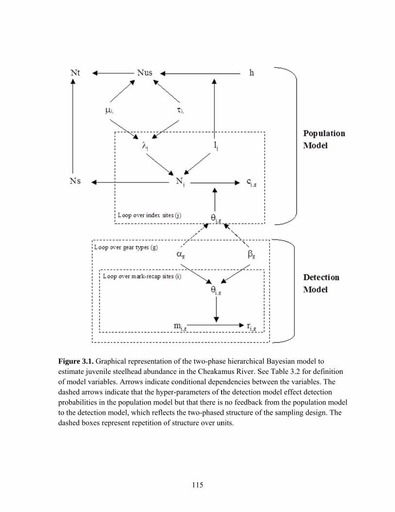
Figurestimof modasheprobato thedashe

re 3.1. Grapmate juvenileodel variableed arrows inabilities in the detection med boxes rep

hical represe steelhead abes. Arrows indicate that thhe populationmodel, whichpresent repeti

entation of thbundance in ndicate condhe hyper-parn model but h reflects theition of struc

115

he two-phasthe Cheakam

ditional deperameters of tthat there is

e two-phasedcture over un

se hierarchicmus River. S

endencies bethe detections no feedbackd structure onits.

al Bayesian See Table 3.etween the van model effek from the p

of the sampli

model to .2 for definitariables. The

ect detection population mng design. T

tion e

model The

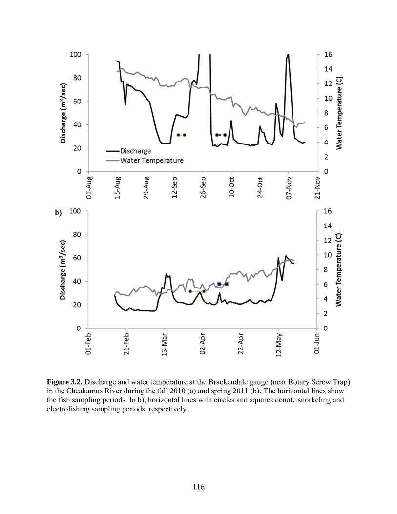
Figure 3in the Chthe fish selectrofis

.2. Dischargheakamus Risampling pershing sampli

ge and water iver during thriods. In b), hing periods,

temperaturehe fall 2010horizontal lirespectively

116

e at the Brac(a) and sprines with circ

y.

ckendale gauing 2011 (b)cles and squ

uge (near Ro. The horizo

uares denote

otary Screw Tontal lines sh

snorkeling a

Trap) how and

Figure 3.3. seasons. Diselectrofishinsnorkeling o

Interannual comstributions from ng and snorkellinonly).

mparisons of lenfall samples are

ng for all Cheak

ngth frequency de based on electkamus River sam

117

distributions for trofishing only wmples and Brohm

juvenile steelhewhile distributiom 2010 and 201

ead between yeaons for spring sa11 only (Brohm

ars within riversamples are based2009 sample ba

s and d on ased on

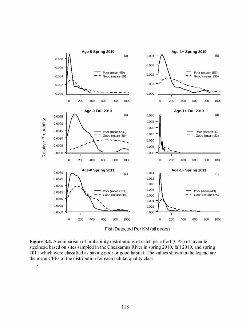
118

Figure 3.4. A comparison of probability distributions of catch per effort (CPE) of juvenile steelhead based on sites sampled in the Cheakamus River in spring 2010, fall 2010, and spring 2011 which were classified as having poor or good habitat. The values shown in the legend are the mean CPEs of the distribution for each habitat quality class.

.

0 200 400 600 800 1000

0.000

0.002

0.004

0.006

0.008

Age-0 Spring 2010

Poor (mean=59)Good (mean=191)

(a)

0 200 400 600 800 1000

0.000

0.001

0.002

0.003

0.004Age-1+ Spring 2010

Poor (mean=153)Good (mean=330)

(b)

0 200 400 600 800 1000

0.0000

0.0005

0.0010

0.0015

0.0020

0.0025

Age-0 Fall 2010

Poor (mean=232)Good (mean=884)

(c)

0 200 400 600 800 1000

0.000

0.005

0.010

0.015

0.020

0.025

0.030Age-1+ Fall 2010

Poor (mean=14)Good (mean=82)

(d)

0 200 400 600 800 1000

0.0000

0.0005

0.0010

0.0015

0.0020

0.0025

0.0030Age-0 Spring 2011

Poor (mean=174)Good (mean=284)

(e)

0 200 400 600 800 1000

0.000

0.002

0.004

0.006

0.008

0.010

0.012

0.014Age-1+ Spring 2011

Poor (mean=43)Good (mean=125)

(f)

Fish Detected Per KM (all gears)

Re

lativ

e P

rob

ab

ility

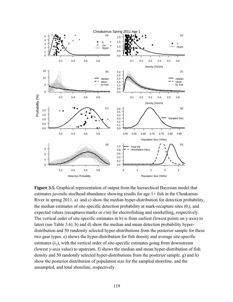
119

Figure 3.5. Graphical representation of output from the hierarchical Bayesian model that estimates juvenile steelhead abundance showing results for age 1+ fish in the Cheakamus River in spring 2011. a) and c) show the median hyper-distribution for detection probability,

the median estimates of site-specific detection probability at mark-recapture sites (i), and expected values (recaptures/marks or r/m) for electrofishing and snorkelling, respectively. The vertical order of site-specific estimates in b) is from earliest (lowest points on y-axis) to latest (see Table 3.6). b) and d) show the median and mean detection probability hyper-distribution and 50 randomly selected hyper-distributions from the posterior sample for these two gear types. e) shows the hyper-distribution for fish density and average site-specific

estimates (j), with the vertical order of site-specific estimates going from downstream (lowest y-axis value) to upstream. f) shows the median and mean hyper-distribution of fish density and 50 randomly selected hyper-distributions from the posterior sample. g) and h) show the posterior distribution of population size for the sampled shoreline, and the unsampled, and total shoreline, respectively.

0.2 0.4 0.6 0.8

0

1

2

3

4

5

i

r/mHyper

(a)

0.2 0.4 0.6 0.8

0

5

10

15

medianmeanby trial

(b)

0.2 0.4 0.6 0.8

0.0

0.5

1.0

1.5

2.0(c)

0.2 0.4 0.6 0.8

0

1

2

3

Detection Probability

(d)

0.1 0.2 0.3 0.4 0.5 0.6

0.0

0.5

1.0

1.5

2.0

Density (f ish/m)

j

Hyper

(e)

0.1 0.2 0.3 0.4 0.5 0.6

0.00.51.01.52.02.53.0

Density (f ish/m)

medianmeanby trial

(f)

0.55 0.60 0.65 0.70 0.75 0.80 0.85

0.00.10.20.30.40.50.6

Population Size ('000s)

Sampled (Ns)

(g)

0 1 2 3 4

0.0

0.2

0.4

0.6

0.81.0

Population Size ('000s)

Total (N)Unsampled (Nus)

(h)

Cheakamus Spring 2011 Age 1

Pro

babi

lity

(%)

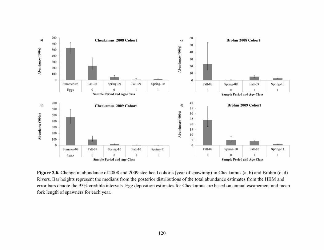
Figure 3.6. Rivers. Bar herror bars defork length o

Change in abunheights represenenote the 95% cof spawners for

ndance of 2008 ant the medians fredible intervalseach year.

and 2009 steelhefrom the posterios. Egg depositio

120

ead cohorts (yeaor distributions

on estimates for

ar of spawning)of the total abunCheakamus are

) in Cheakamus undance estimatee based on annu

(a, b) and Brohmes from the HBMal escapement a

m (c, d) M and and mean

Figurexperlimitsmark

re 3.7. Averriments for as. Numbers a

ks applied acr

rage detectioage-0 and -1+at the top of ross all expe

on probability+ steelhead b

f the figure deriments (M)

121

y for electroby habitat ty

denote the nu).

ofishing-baseype. Eror barumber of exp

ed mark-recars denote 95periments (N

apture % confidenc

N) and the toce tal

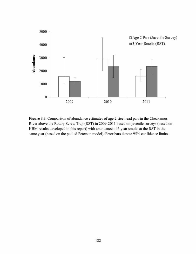
FigurRiverHBMsame

re 3.8. Compr above the R

M results dev year (based

parison of abRotary Screw

veloped in thd on the pool

bundance esw Trap (RSTis report) wiled Peterson

122

stimates of agT) in 2009-20ith abundancmodel). Err

ge 2 steelhea011 based once of 3 year ror bars deno

ad parr in thn juvenile susmolts at theote 95% con

he Cheakamuurveys (basee RST in thefidence limi

us ed on e ts.