The Impacts of Neighborhoods on Intergenerational Mobility:

Childhood Exposure E↵ects and County-Level Estimates

Raj Chetty and Nathaniel HendrenHarvard University and NBER

May 2015

Abstract

We characterize the e↵ects of neighborhoods on children’s earnings and other outcomes in adult-hood by studying more than five million families who move across counties in the U.S. Ouranalysis consists of two parts. In the first part, we present quasi-experimental evidence thatneighborhoods a↵ect intergenerational mobility through childhood exposure e↵ects. In partic-ular, the outcomes of children whose families move to a better neighborhood – as measured bythe outcomes of children already living there – improve linearly in proportion to the time theyspend growing up in that area. We distinguish the causal e↵ects of neighborhoods from con-founding factors by comparing the outcomes of siblings within families, studying moves triggeredby displacement shocks, and exploiting sharp variation in predicted place e↵ects across birthcohorts, genders, and quantiles. We also document analogous childhood exposure e↵ects forcollege attendance, teenage birth rates, and marriage rates. In the second part of the paper, weidentify the causal e↵ect of growing up in every county in the U.S. by estimating a fixed e↵ectsmodel identified from families who move across counties with children of di↵erent ages. We usethese estimates to decompose observed intergenerational mobility into a causal and sorting com-ponent in each county. For children growing up in families at the 25th percentile of the incomedistribution, each year of childhood exposure to a one standard deviation (SD) better countyincreases income in adulthood by 0.5%. Hence, growing up in a one SD better county frombirth increases a child’s income by approximately 10%. Low-income children are most likely tosucceed in counties that have less concentrated poverty, less income inequality, better schools,a larger share of two-parent families, and lower crime rates. Boys’ outcomes vary more acrossareas than girls, and boys have especially poor outcomes in highly-segregated areas. In urbanareas, better areas have higher house prices, but our analysis uncovers significant variation inneighborhood quality even conditional on prices.

The opinions expressed in this paper are those of the authors alone and do not necessarily reflect the views of theInternal Revenue Service or the U.S. Treasury Department. This work is a component of a larger project examiningthe e↵ects of tax expenditures on the budget deficit and economic activity. All results based on tax data in thispaper are constructed using statistics originally reported in the SOI Working Paper “The Economic Impacts of TaxExpenditures: Evidence from Spatial Variation across the U.S.,” approved under IRS contract TIRNO-12-P-00374and presented at the Oce of Tax Analysis on November 3, 2014. We thank David Autor, Gary Chamberlain, MaxKasy, Lawrence Katz, and numerous seminar participants for helpful comments and discussions. Sarah Abraham,Alex Bell, Augustin Bergeron, Jamie Fogel, Nikolaus Hildebrand, Alex Olssen, Benjamin Scuderi, and Evan Stormsprovided outstanding research assistance. This research was funded by the National Science Foundation, the Lab forEconomic Applications and Policy at Harvard, and Laura and John Arnold Foundation.

I Introduction

To what extent are children’s opportunities for economic mobility shaped by the neighborhoods

in which they grow up? Despite extensive research, the answer to this question remains debated.

Observational studies by sociologists have documented significant variation across neighborhoods

in economic outcomes (e.g., Wilson 1987, Sampson et al. 2002, Sharkey and Faber 2014). However,

experimental studies of families that move have found little evidence that neighborhoods a↵ect

economic outcomes (e.g., Katz et al. 2001, Oreopoulos 2003, Ludwig et al. 2013).

In this paper, we present new quasi-experimental evidence on the e↵ects of neighborhoods on

intergenerational mobility and reconcile the conflicting findings of prior work. Our analysis, which

uses data from de-identified tax records covering the U.S. population from 1996-2012, consists of

two parts.

Part I: Quasi-Experimental Evidence of Childhood Exposure E↵ects. In the first part of this

paper, we measure the degree to which the di↵erences in intergenerational mobility across areas

documented in observational studies are driven by causal e↵ects of place. In previous work (Chetty,

Hendren, Kline, and Saez 2014), we documented substantial variation across commuting zones in

children’s expected earnings (measured by their percentile rank in the national income distribution)

conditional on their parents’ income.1 This geographic variation in intergenerational mobility could

be driven by two very di↵erent sources. One possibility is that neighborhoods have causal e↵ects

on economic mobility: that is, moving a given child to a di↵erent neighborhood would change her

life outcomes. Another possibility is that the observed geographic variation is due to systematic

di↵erences in the types of people living in each area, such as di↵erences in demographic makeup or

wealth.

We test these explanations and identify the causal e↵ects of neighborhoods by studying more

than five million families who move across counties and exploiting di↵erences in their children’s ages

when they move. We first show that children whose parents move to a better neighborhood – i.e., a

CZ or county where children of permanent residents (non-movers) at their income percentile have

higher earnings in adulthood – earn more themselves.2 Symmetrically, those who move to worse

1We characterize neighborhood (or “place”) e↵ects at two geographies: counties and commuting zones (CZs),which are aggregations of counties that are similar to metro areas but cover the entire U.S., including rural areas.Naturally, the variance of place e↵ects across these broad geographies is a lower bound for the total variance ofneighborhood e↵ects, which would include additional local variation.

2We measure children’s incomes between the ages of 24 and 30; our results are not sensitive to varying the age atwhich child income is measured within this range.

1

neighborhoods have lower earnings as adults.3 Importantly, the changes in earnings are proportional

to the fraction of childhood spent in the new area. On average, spending an extra year in a CZ

or county where the mean rank of children of permanent residents is 1 percentile higher increases

a child’s expected rank by approximately 0.03-0.04 percentiles. Stated di↵erently, the outcomes of

children who move converge to the outcomes of permanent residents of the destination area at a

rate of approximately 3-4% per year of exposure.

Under the assumption that the timing of parents’ moves is orthogonal to children’s potential

outcomes – an assumption that we revisit and validate below – this convergence pattern implies

that neighborhoods have substantial childhood exposure e↵ects. That is, every additional year of

childhood spent in a better environment improves a child’s long-term outcomes. The convergence

is linear with respect to age: moving to a better area at age 8 instead of 9 is associated with the

same improvement in earnings as moving to that area at age 15 instead of 16. The exposure e↵ects

persist until children are in their early twenties. Extrapolating over the duration of childhood, from

age 0 to 20, the roughly 3.5% annual convergence rate implies that at least 50% and as much as

70% of the variance in observed intergenerational mobility across counties and commuting zones is

due to the causal e↵ects of place.4 We find analogous childhood exposure e↵ects for several other

outcomes, including college attendance, teenage employment, teenage birth, and marriage.

The critical identification assumption underlying our approach is that children whose parents

move to a better (or worse) area at a young age have comparable potential outcomes to children

whose parents move when they are older. This orthogonality condition would be violated if, for

instance, parents who move to a better area when their children are young are wealthier or invest

more in their children. In addition, moving may itself be correlated with other factors – such as

a higher-paying job or a change in marital status – that directly a↵ect children in proportion to

exposure time. We use three approaches to account for such selection and omitted variable biases:

controlling for observable factors, isolating moves triggered by exogenous events, and implementing

a set of sharp placebo (or overidentification) tests.

We control for factors that are fixed within the family (e.g., parent education) by including fam-

ily fixed e↵ects when estimating exposure e↵ects, as in Plotnick and Ho↵man (1996) and Aaronson

3Throughout the paper, we refer to areas where children have better outcomes in adulthood as “better” neigh-borhoods. We use this terminology without any normative connotation, as there are of course many other amenitiesof neighborhoods that may be relevant from a normative perspective.

4Formally, 0.035*20 = 70% is a point estimate under the assumption that the causal e↵ects and sorting componentsare uncorrelated. Without this assumption, the variance of predicted values, (0.035 20)2 = 0.49, provides a lowerbound.

2

(1998). This approach identifies exposure e↵ects from comparisons between siblings, e↵ectively ask-

ing whether the di↵erence in outcomes between two siblings in a family that moves is proportional

to the size of the age gap between them. We obtain an annual exposure e↵ect of approximately 4%

per year with family fixed e↵ects, very similar to our baseline estimates. Controlling for parents’

incomes and marital status in each year also has no e↵ect on the estimates.

Of course, one may still be concerned that whatever unobserved change induced a family to move

(e.g., a wealth shock) may also have had direct e↵ects on their children’s outcomes. To account

for such unobserved factors, we next focus on a subset of moves where we have more information

what caused the move. We identify moves that occur as part of large outflows from ZIP codes,

which are typically caused by natural disasters or local plant closures. To remove the endogeneity

of individual choice – for example, wealthier parents with young children sorting to better areas in

response to the shock – we instrument for the change in neighborhood quality using the average

change in neighborhood quality of those who move out of the ZIP code during the years in our

sample. Once again, we obtain exposure e↵ect estimates similar to the baseline in this subsample

displaced by such exogenous shocks.

While the instrumental variables approach further validates the baseline exposure e↵ect design

in the small subset of areas that experience displacement shocks, our ultimate goal is to develop

credible estimates of exposure e↵ects for all areas in the U.S. We therefore turn to a third approach

– implementing placebo (overidentification) tests that exploit heterogeneity in place e↵ects across

subgroups – which in our view is ultimately the most compelling method of assessing the validity

of the design. We begin by analyzing heterogeneity in place e↵ects across birth cohorts. Although

there is considerable persistence in outcomes within CZs over time, some places improve and others

decline. Exploiting this variation, we show that, in a multivariable regression, the outcomes of

children who move to a new area converge to the outcomes of permanent residents of the destination

in their own birth cohort but not those of surrounding birth cohorts (conditional on their own birth

cohort predictions). It would be unlikely that sorting or omitted variables would produce such a

sharp cohort-specific pattern, especially because the cohort-specific e↵ects are only observed ex-post

after children grow up. Hence, this evidence of cohort-specific convergence supports the view that

our neighborhood exposure e↵ect estimates are not confounded by selection and omitted variable

biases.

Next, we implement analogous placebo tests by exploiting variation in the distribution of out-

comes, as opposed to focusing solely on mean outcomes. For instance, low-income children who

3

spend their entire childhood in Boston or San Francisco have similar outcomes on average, but

children in San Francisco are more likely to end up in the upper tail (top 10%) or lower tail (bot-

tom 10%) of the income distribution. The causal exposure e↵ects model predicts convergence not

just at the mean but across the entire distribution; in contrast, it would be quite unlikely that

omitted variables (such as changes in parent wealth) would happen to perfectly replicate the entire

distribution of outcomes in each area. In practice, we find clear evidence of distributional conver-

gence: controlling for mean outcomes, children’s outcomes converge to predicted outcomes in the

destination across the distribution in proportion to exposure time, again at a rate of approximately

3.5% per year.

Finally, we find analogous results when analyzing heterogeneity in outcomes across genders.

Though place e↵ects are highly correlated for boys and girls, there are some di↵erences in predicted

outcomes by gender across neighborhoods. For instance, highly-segregated areas tend to have lower

mean outcomes for boys than girls. We find that when a family with both a daughter and a son

moves to an area that is particularly good for boys, their son’s outcomes improve in proportion to

exposure time to the destination much more than their daughter’s outcomes. Once again, if our

findings were driven by sorting or omitted variables, one would not expect to find stark di↵erences

in impacts by gender unless families’ unobservable investments in their children are di↵erentially

correlated with where they move.

Overall, these results suggest that neighborhoods matter for children’s long-term outcomes and

suggest that at least half of the variance in observed intergenerational mobility across areas is due

to the causal e↵ect of place. But, it does not directly tell us which areas produce the best outcomes.

In the second part of this paper, we address this question by estimating the causal e↵ect of each

county and commuting zone (CZ) in the U.S. on children’s earnings in adulthood.

Part II: County-Level Estimates of Causal E↵ects. We estimate each CZ and county’s causal

e↵ect on children’s incomes and characterize the properties of areas that produce good outcomes

in four steps.

First, we estimate the fixed e↵ect for each county (or CZ) using a regression model that is

identified from families who move across areas with children of di↵erent ages. To understand

how the model is identified, consider families in the New York area. If children who moved from

Manhattan to Queens at younger ages earn more as adults, we can infer that Queens has positive

childhood exposure e↵ects relative to Manhattan under our central assumption that the timing of

families’ moves are orthogonal to their children’s potential outcomes. Building on this logic, we

4

use our sample of cross-county movers to regress children’s earnings in adulthood on fixed e↵ects

for each county interacted with the fraction of childhood spent in that county. We estimate the

county fixed e↵ects separately by parent income level, permitting the e↵ects of each area to vary

with family income. We also include origin by destination fixed e↵ects when estimating this model,

so that each county’s e↵ect is identified purely from di↵erences in the age of the children when

families move across areas.

In the second step of our analysis, we estimate the variance components of a latent variable

model of neighborhood e↵ects, treating the fixed e↵ects as the sum of a latent causal e↵ect and

noise due to sampling error. We estimate the signal variance of neighborhood e↵ects by subtracting

the portion of the variance in the fixed e↵ects due to noise. For a child with parents at the 25th

percentile of the national income distribution, we estimate that spending one additional year of

childhood in a one SD better county (population weighted) increases household income at age 26 by

0.17 percentile points, which is approximately equivalent to an increase in mean earnings of 0.5%.

Extrapolating over 20 years of childhood, this implies that growing up in a 1 SD better county

from birth would increase a child’s income in adulthood by approximately 10%.

Neighborhoods have similar e↵ects in percentile rank or dollar terms for children of higher-

income parents, but matter less in percentage terms because children in high-income families have

higher mean earnings. For children with parents at the 75th percentile of the income distribution,

the signal SD of annual exposure e↵ects across counties is 0.16 percentiles, which is approximately

0.3% of mean earnings. Areas that produce better outcomes for children in low-income families are,

on average, no worse for those from high-income families. This finding suggests that the success of

the poor in certain areas of the U.S. does not necessarily come at the expense of the rich.

Our estimates imply that roughly two-thirds of the variation in intergenerational mobility across

counties documented in (Chetty et al., 2014) for children in low-income (25th percentile) families

is driven by causal e↵ects. The remaining one third is driven by sorting, i.e. systematic di↵erences

in the characteristics of the people living in each county. The causal and sorting components

are approximately uncorrelated with each other: there is no evidence that families with better

unobservables systematically sort to better counties conditional on parent income in equilibrium.

The variance components of our model of neighborhood e↵ects allow us to quantify the degree

of signal vs. noise in each CZ and county’s fixed e↵ect estimate. In CZs and counties with large

populations, such as Cook County in Chicago, the signal accounts for 75% of the variance in the

fixed e↵ect estimate. However, in smaller counties, more than half of the variance in the fixed e↵ect

5

estimates is due to noise. As a result, the raw fixed e↵ects are not appropriate for forming forecasts

of each county’s causal e↵ect for most counties.

In the third step of our analysis, we construct forecasts of each county’s causal e↵ect using a

simple shrinkage estimator. We construct the best (minimum mean-squared-error) linear prediction

of each county’s causal e↵ect by taking a weighted average of the fixed e↵ect estimate based on

the movers and a prediction based on permanent residents’ outcomes. The permanent residents’

mean outcomes have very little sampling error, but are imperfect predictors of a county’s causal

e↵ect because they combine causal e↵ects with sorting. Therefore, in large counties, where the

degree of sampling error in the fixed e↵ect estimates is small, the optimal predictor puts most of

the weight on the fixed e↵ect estimate based on the movers. In smaller counties, where the fixed

e↵ects estimates are very imprecise, the estimator puts more weight on the predicted outcome

based on the permanent residents. The county-level predictions obtained from this procedure yield

unbiased forecasts of the impacts of each county in the sense that moving a child to a county with

a 1 percentile higher predicted e↵ect will increase that child’s earnings in adulthood by 1 percentile

on average.

We use our county-level forecasts to identify the best and worst counties in the U.S. in terms of

their causal e↵ects on intergenerational mobility. Each additional year that a child spends growing

up in Dupage County, IL – the highest-ranking county in terms of its causal e↵ect on upward

mobility among the 100 largest counties in the U.S. raises her household income in adulthood by

0.80%. This implies that growing up in Dupage County from birth – i.e., having about 20 years

of exposure to that environment – would raise a child’s earnings by 16% relative to the national

average. In contrast, every extra year spent in the city of Baltimore – one of the lowest-ranking

counties – reduces a child’s earnings by 0.7% per year of exposure, generating a total earnings

penalty of approximately 14% for children who grow up there from birth.5

Our estimates of causal e↵ects at the county and commuting zone (CZ) level are highly correlated

with the raw statistics on intergenerational mobility reported in (Chetty et al., 2014), but there are

several significant di↵erences. For example, children who grow up in New York City have above-

average rates of upward mobility. However, the causal e↵ect of growing up in New York City on

upward mobility – as revealed by analyzing individuals who move into and out of New York – is

negative relative to the national average. This negative e↵ect of growing up in New York is masked

5These estimates are based on data for children born between 1980-86 and who grew up in the 1980’s and 1990’s.We find that neighborhoods’ e↵ects generally remain stable over time, but some cities have presumably gotten betterin the 2000’s, while others may have gotten worse.

6

when one simply studies the average outcomes of children who grow up there because families who

live in New York tend to have unusually high rates of upward mobility. In particular, New York has

a very large share of immigrants, and we find evidence consistent with immigrants having higher

rates of upward mobility independent of where they live.

We find that neighborhoods matter more for boys than girls: the signal SD of county-level

e↵ects for boys is roughly 1.5-times that of girls in low-income (25th percentile) families. Moreover,

the distribution of county-level forecasts is wider and has a thick lower-tail for boys, with some

counties such as Baltimore and Wayne County in Detroit producing extremely negative outcomes

for boys but less so for girls. Areas with high degrees of segregation and sprawl generate particularly

negative outcomes for boys relative to girls. There are also significant gender di↵erences related to

marriage rates. For example, Northern California generates high levels of individual earnings for

girls, but produces lower levels of household income because fewer children get married in their 20s.

What are the properties of areas that improve upward mobility? In the last step of our analysis,

we characterize the properties of counties and CZs that produce good outcomes by correlating the

estimated causal and sorting e↵ects with observable characteristics. Within CZs, counties that

produce better outcomes for children in low-income families tend to have five characteristics: lower

rates of residential segregation by income and race, lower levels of income inequality, better schools,

lower rates of violent crime, and a larger share of two-parent households. For high income families,

we find positive correlations with school quality, social capital, and inequality. But, we find measures

of segregation and poverty are not strongly correlated with the causal e↵ects of counties on high-

income families. However, they are strongly correlated with the sorting component for high-income

families, implying that high-income families with good unobservables tend not to live in cities that

generate worse outcomes for the poor (such as segregated areas).

Urban areas, particularly those with substantial concentrated poverty, typically generate much

worse outcomes for children than suburbs and rural areas for both low- and high-income families.

We also find that areas with a larger African-American population tend to have lower rates of

upward mobility. These spatial di↵erences amplify racial inequality across generations: we estimate

that roughly one-fifth of the gap in earnings between blacks and whites can be attributed to the

counties in which they grow up.

Finally, we evaluate how much more one has to pay in terms of housing costs to live in areas

that generate good outcomes for children. Across CZs, we find a negative correlation with housing

prices, as rural areas have low house prices and tend to produce better outcomes. However, across

7

counties within CZs, counties that o↵er better prospects for children have higher house prices and

rents. The correlation between rents and children’s outcomes is particularly strong in cities that

have high levels of segregation and sprawl, which may explain the persistence of poverty across

generations in such cities.

Although rents are correlated with upward mobility in large cities, there are some bargains to

be found. For example, in the New York metro area, Hudson County, New Jersey o↵ers much

higher levels of upward mobility than Queens or the Bronx even though median rents in that area

are comparable to the New York boroughs over the period we study. If we divide neighborhood

e↵ects into the component that projects onto observable factors such as poverty and dropout rates

and the residual “unobservable” component, only the observable component is capitalized in rents

and house prices. Our findings show that there is substantial scope for households to move to areas

within their CZ that produce better outcomes for children without paying higher rents, and our

estimates provide guidance in identifying such areas empirically.

Our findings help reconcile the conflicting results in the prior literature on neighborhood e↵ects,

most notably the discrepancy between the findings from the Moving to Opportunity Experiment and

observational studies documenting substantial variation in children’s outcomes across areas even

after controlling for observable di↵erences in characteristics. Prior analyses of the MTO experiment

have focused primarily on the e↵ects of neighborhoods on adults and older youth (e.g. Kling et al.

(2007)) and have not explicitly tested for exposure e↵ects among children. In a companion paper

(Chetty, Hendren, and Katz, 2015), we link the MTO data to tax records and show that the

MTO data exhibit the same exposure time patterns as those we document here. In particular, we

find large treatment e↵ects for children who moved to better neighborhoods at young ages but not

those who moved at older ages. More generally, our findings imply that much of the variation across

neighborhoods documented in observational studies does in fact reflect causal e↵ects of place, but

that these e↵ects arise through accumulated childhood exposure rather than impacts on adults.

The rest of the paper is organized as follows. In Section II, we present a stylized model of

neighborhood e↵ects to formalize our empirical objectives. Section III describes the data. Sections

IV-VI present the analysis underlying the first part of the paper. Section IV presents baseline

estimates of average neighborhood exposure e↵ects on earnings by studying the e↵ects of moving

to areas where prior permanent residents are doing better (or worse). Section V presents a series

of tests validating our baseline identification assumptions and Section VI presents estimates of

exposure e↵ects for other outcomes. Sections VII-X comprise the second part of our analysis.

8

Section VII presents the fixed e↵ect estimates based on movers. Section VIII presents estimates

of the variance components of the neighborhood e↵ects model. Section IX presents our forecasts

of each county and CZs causal e↵ect based on the shrinkage estimator. In Section X, we correlate

the estimated place e↵ects with observables. Section XI concludes and discusses our findings in the

context of prior work. Estimates of neighborhood e↵ects and related covariates are available by

commuting zone and county on the project website.

II Model and Empirical Objectives

We begin with a stylized model of neighborhood e↵ects and location choice. We use this model

to define the estimands of interest, derive estimating equations, and formalize the identification

assumptions underlying our research design.

II.A Setup

Consider a discrete time model in which parents live for T periods. Children i = 1, ..., I are born

in year t = 1 and leave their parents’ household and enter the labor market in year TC . Let yi

denote a long-term outcome (e.g., earnings in adulthood) of child i. Let f(i) denote the family to

which child i is born; we allow multiple children per family to compare siblings’ outcomes. Let

p(f(i)) the percentile rank of child i’s parents in the national income distribution, and c(f(i), t)

the neighborhood in which his family lives in year t. We treat parent income p(i) = p(f(i)) as

exogenous and fixed over time.6 Our model consists of a specification for the production function

for children’s outcomes yi and the parents’ choice of location c(i, t) in each period.

Children’s outcomes yi are a function of neighborhood characteristics, family inputs, and disrup-

tion costs of moves during childhood. Let µpc denote the causal e↵ect of growing up in neighborhood

c for one’s entire childhood (i.e., from periods 1 to TC) for a child with parents at percentile p.

Allowing neighborhoods to have heterogeneous e↵ects across the parent income distribution turns

out to be important empirically. Let it denote the family inputs in year t, which we interpret as

a combination of active investments by parents (e.g., via financial resources or time) and variation

in latent ability (e.g., due to genetics). We model the child’s outcome yi as an additive function

of the neighborhood and family inputs she receives over her childhood net of disruption costs of

6In our empirical analysis, we show this assumption does not a↵ect our results by controlling for changes in incomeand measures of income separately by year.

9

moves:

yi = i +TCX

t=1

[tµp(i),c(f(i),t) tIc(i, t) 6= c(i, t 1)], (1)

where i =PT

C

t=11TC

it is the mean level of parental inputs to child i and Ic(i, t) 6= c(i, t 1)

denotes an indicator for having moved neighborhoods in year t. The weights t allow for the

possibility that some periods of a child’s life may be more important than others for long-term

development, where t > 1 (t < 1) indicates year t is relatively more (less) important than other

years of childhood. Let m =P

mt=1t denote the cumulative sum of growing up in a one-unit

better area from birth to age m. We normalize Tc

=PT

C

t=1 t = TC . Equation (1) imposes that

the parent’s location c(i, t) after the child has left the house (t > TC) has no causal e↵ect on the

child’s outcome – an assumption we test below. The coecients t measure the disruption cost of

moving neighborhoods at year (or age) t, with 1 0.

The production function for yi in (1) imposes two substantive restrictions that are relevant for

our empirical analysis. First, it assumes that neighborhood e↵ects are additive, i.e. there are no

complementarities between neighborhood quality across years, and do not vary across individuals

conditional on parent income p.7 Second, it assumes that the disruption costs of moving t do

not vary across neighborhoods.8 Equation (1) does allow for critical ages in which neighborhood

outcomes may be more important (by varying t), and in our baseline analysis we allow for these

di↵erences. However, for many outcomes, our empirical findings will suggest that a simpler linear

exposure time specification with t = 1 fits the data quite well:

yi = i +X

c

mi,cµpc + i (2)

where i is the mean of parental inputs,P

cmi,cµpc is the sum of exposure e↵ects9 where mi,c

is the number of years (of childhood, t TC) that child i spends in neighborhood c, and i =PT

C

t=11T tI c (i, t) 6= c (i, t 1) is the net impact of moving disruptions.

While we do not attempt to estimate a utility function over parents’ choice of neighborhoods

and investments in children, it is useful for some of our empirical tests below10 to conceptualize

7We defer the identification of complementarities and heterogeneity to future work. If the true production functionfeatures complementarities or heterogeneity, our reduced-form empirical estimates of µ

pc

can be interpreted as themean e↵ect of spending an extra year in area c for the individuals who move to c from other areas.

8The key assumption for identification of µpc

will be that t

cannot vary in a di↵erentially age-dependent manneracross neighborhoods; it is feasible to extend the model to allow for disruption cost that varies across neighborhoodsbut for which the age-gradient of

t

does not vary across neighborhoods.9Note that

PTCt=1 t

µ

p(i),c(f(i),t) =P

c

m

i,c

µ

pc

if t

= 1 for all t.10Specifically, in Section V.C we provide tests of our identification of neighborhood e↵ects by exploiting restrictions

on the parents’ information set, , in how neighborhoods can a↵ect their children’s outcomes in adulthood.

10

parents making decisions to maximize their expected utility. We imagine that parents of child

i, f (i), choose neighborhoods, c (f (i) , t), to maximize some lifetime utility function of children’s

outcomes, parent inputs, and other neighborhood- and time-specific factors:

EhUf (

!yf ,

!f ,

!f )|

i(3)

where !yf = yi|f(i) = f denotes the vector of outcomes for the children in family f ,

!f =

it|f(i) = f is the vector of family inputs, and !f = (f,c(f,1), ...,f,c(f,t)) denotes other factors

that vary across neighborhoods and time, such as local amenities, job opportunities and proxim-

ity to work, and local house prices. Parents choose a sequence of investment levels (1, ..., TC

)

and neighborhoods c(i, 1), ..., c(i, T ) to maximize their expected utility Uf given their resource

constraints and knowledge, , about how their choices a↵ect outcomes.

II.B Empirical Objectives

Objective #1. Our empirical analysis has two objectives, which we define here using (hypothet-

ical) randomized experiments. Our first objective is directly motivated by the current debate in

the literature on neighborhood e↵ects. Prior work has documented robust di↵erences in children’s

outcomes yi across neighborhoods in observational data (e.g., Wilson 1987, Jencks and Mayer 1990,

Massey 1993, Brooks-Gunn et al. 1993, Cutler et al. 1997, Leventhal and Brooks-Gunn 2000, Samp-

son et al. 2002 ). But experimental evidence to date finds little evidence that moving children to

better neighborhoods – e.g., those with lower poverty rates – improves outcomes. Therefore, our

first goal is to determine whether moving to an area in which other children do well has a causal

e↵ect on children’s outcomes and to provide a lower bound on the fraction of the variation in

observed economic outcomes reflects the causal e↵ects of neighborhoods.

To formalize our first question, observe that the mean outcome of children who spend their

entire childhood in area c is ypc = TCµpc + pc, where pc = E[ 1TPit|c(i, t) = c] is the mean level

of investment in children by families who live in that area and TCµpc is the cumulative e↵ect of

childhood exposure to area c. Mean parent investments pc vary across areas due to endogenous

parent sorting and may be correlated with µpc.11 We are interested in whether and by how much

the mean outcomes across places reflect the causal impacts of those places. In other words, we seek

to estimate E [µpc|ypc].11For example, parents who place higher weight on their children’s outcomes may choose to live in areas that are

better for their child (higher µpc

) and also invest more in their child directly (higher it

), leading to Cov(µpc

,

pc

) > 0in equilibrium. Conversely, parents may choose to invest in neighborhoods as a substitute for other investments,leading to Cov

µ

pc

,

pc

< 0.

11

One intuitive way to answer this question would be to randomly assign children to neighborhoods

at a given age m2[1, TC ] and estimate the best linear predictor of children’s outcomes yi in the

experimental sample using ypc :

yi = ↵+ mypc + "i (4)

Given estimates! = mTC

m=1, we define the exposure e↵ect of moving to a better area at age m

by m m1. Under the simple a linear exposure model in equation (2), the exposure e↵ect is

constant and given by m m1 = E [µpc|ypc] for all m.12

Estimating exposure e↵ects (i.e. the pattern of m across di↵erent ages, m) provides answers

to several questions. First, finding a positive e↵ect (at any age) allows us to reject the null that

neighborhoods do not matter, a null of interest given experimental evidence to date. Second, the

values of the exposure e↵ects at di↵erent ages are informative about the ages at which neighborhood

environments matter most for children’s outcomes.13 Finally, the magnitude of 1 – the impact

of assigning children to better neighborhood from birth – yields bounds on the variance of place

e↵ects, 2µp = V ar(µpc):T

2c

2µp

2yp

21 (5)

Intuitively, the variance of predicted e↵ects based on permanent resident outcomes ypc, 212yp

is

a lower bound for the total variance of place e↵ects, T 2c

2µp, of obtaining an entire childhood (Tc

years) of exposure to the place e↵ect.14 Under an additional assumption of no covariance between

the sorting and causal components (µp and i), 1 is exactly equal to the fraction of variance that

is due to the causal e↵ect, 1 =T 2c

2µ

p

2y

p

.15

Another key advantage of estimating E [µpc|ypc] is that it will facilitate a range of high pow-

ered placebo (overidentification) tests that utilize the information contained in the distribution of

12We assume that does not vary across parent income percentiles p to simplify notation, but one could estimate(4) separately by p to identify a coecient

p

for each p. In our empirical application, we show that p

does not varysignificantly across percentiles.

13More precisely, the pattern of m

identifies the ages at which moving to a better environment, as measured bythe outcomes of prior residents, has the largest e↵ects. Other measures of the quality of a child’s environment couldpotentially generate di↵erent critical ages.

14To see this, we can use (1) to write the outcome of a child who is randomly assigned to a neighborhood c at agem as

y

i

= (Tc

m

)µpc

m

+

i

, (6)

where E[i

|c] = 0 (the neighborhood e↵ect before age m is subsumed in the error term

i

because of ran-dom assignment). To see that that 2

µp T

2c

V ar(1ypc) = T

2c

21

2yp , note that V ar(1ypc) =

21V ar(y

pc

) =

Cov(Tc

µ

pc

, y

pc

)/2ypc =

2µp

Cov(Tcµpc,ypc)

2ypc

2µp

= T

2c

2µp

2µpcypc T

2c

2µp because the correlation coecient

µpcypc 1.15To see this, note that

1 =cov (T

c

µ

pc

, y

pc

)var (y

pc

)=

T

2c

2µpc

2ypc

12

outcomes of permanent residents in an area to test for the presence of bias from sorting patterns

(e.g. families of children with high pc moving to places with high µpc when their kids are young).

But, while! tells us about the average e↵ects of exposure to neighborhoods where prior residents

are doing better, E [µpc|ypc], estimating! itself is not adequate to identify the causal e↵ects of

growing up in each neighborhood c, µpcCc=1.

Objective #2. Our second objective – which we take up in Part II (starting in Section VII) –

is to directly estimate fixed e↵ects for each place µpc to determine the causal impact of an additional

year of exposure to each commuting zone and county in the U.S. The ideal experiment to estimate

µpc would be to randomly assign children at each parent income level p to each neighborhood from

birth. One could then identify each place’s causal e↵ect simply using mean observed outcomes in

each area (µpc = ypc), since random assignment guarantees pc does not vary across places (for all

p).16 In contrast to Objective #1, this does not require any information about the outcomes of

permanent residents, ypc.

In Section VII, we construct unbiased estimates of µpc. We then decompose observed outcomes,

ypc, into causal (µpc) and sorting (pc) components, and estimate the variance of these components

in Section VIII. This exercise breaks up the observed pattern of intergenerational mobility in the

U.S. into a component due to the causal e↵ects of places and a component due to systematic

di↵erences in the types of people living in di↵erent places who provide di↵erential inputs to their

children, i. Next, in Section IX we combine our fixed e↵ect estimates of µpc (identified solely

from movers) with the estimate of E [µpc|ypc] = ypc (identified using information in permanent

resident outcomes) to form a forecast of each place’s causal e↵ect, µfpc, that minimizes mean-square

prediction error and delivers unbiased forecasts. Finally, in Section X we characterize the correlates

of places with high values of µpc by regressing our estimates on observables, such as poverty rates

and local school quality.

The remainder of the paper implements these empirical objectives using observational data on

families who move across neighborhoods.

16In principle, one could go straight to identifying the causal e↵ects of place µpc

without identifying . We donot take this approach for two reasons that we discuss further below: (1) we are able to estimate under weakerorthogonality assumptions than µ

pc

and (2) we obtain much more precise estimates of than µpc

by using data onprior residents’ outcomes to collapse the problem into estimating one parameter rather than estimating thousands ofplace e↵ects. Given that a key question in the literature is whether neighborhoods matter at all, we view credibleestimation of as a critical first step before turning to secondary questions about which neighborhoods are better orworse.

13

III Data, Geographic Definitions, and Summary Statistics

We use data from federal income tax records spanning 1996-2012. The data include both income

tax returns (1040 forms) and third-party information returns (e.g., W-2 forms), which give us

information on the earnings of those who do not file tax returns. Our analysis sample is essentially

identical to that used to study intergenerational mobility in Chetty et al. (2014), and much of

what follows in this section is taken directly from that paper.17 Here, we briefly summarize the key

variable and sample definitions. Note that in what follows, the year always refers to the tax year

(i.e., the calendar year in which the income is earned).

III.A Sample Definitions

Our base dataset of children consists of all individuals who (1) have a valid Social Security Number

or Individual Taxpayer Identification Number, (2) were born between 1980-199118, and (3) are

U.S. citizens as of 2013. We impose the citizenship requirement to exclude individuals who are

likely to have immigrated to the U.S. as adults, for whom we cannot measure parent income. We

cannot directly restrict the sample to individuals born in the U.S. because the database only records

current citizenship status.

We identify the parents of a child as the first tax filers (between 1996-2012) who claim the child

as a child dependent and were between the ages of 15 and 40 when the child was born. If the child is

first claimed by a single filer, the child is defined as having a single parent. For simplicity, we assign

each child a parent (or parents) permanently using this algorithm, regardless of any subsequent

changes in parents’ marital status or dependent claiming.

If parents never file a tax return, we do not link them to their child. Although some low-income

individuals do not file tax returns in a given year, almost all parents file a tax return at some point

between 1996 and 2012 to obtain a tax refund on their withheld taxes and the Earned Income

Tax Credit (Cilke 1998). We are therefore able to identify parents for approximately 95% of the

children in the 1980-1991 birth cohorts. The fraction of children linked to parents drops sharply

prior to the 1980 birth cohort because our data begin in 1996 and many children begin to the leave

the household starting at age 17 (Chetty et al. (2014); Online Appendix Table I). This is why we

17See Online Appendix A of Chetty et al. (2014) for a detailed description of how we construct the analysis samplestarting from the raw population data. The records are complete as of the summer of 2013. This implies they includea complete set of information returns, but potentially exclude some amendments and late filings for 1040s in 2012.Restricting our baseline analysis to use data through 2011 yields very similar results.

18The teen labor outcomes in Figure XI include additional data from children born up to 1996.

14

limit our analysis to children born during or after 1980.

Our full analysis sample includes all children in the base dataset who (1) are born in the 1980-91

birth cohorts, (2) for whom we are able to identify parents, and (3) whose mean parent income

between 1996-2000 is strictly positive (which excludes 1.2% of children).19

Geographic Definitions: We conceptualize neighborhood e↵ects using a hierarchical model in

which children’s outcomes depend upon conditions in their immediate neighborhood (e.g., peers or

resources in their city block), local community (e.g., the quality of schools in their county), and

broader metro area (e.g., local labor market conditions). We characterize neighborhood e↵ects first

at the level of commuting zones (CZs) and then at the level of counties. CZs are aggregations

of counties based on commuting patterns in the 1990 Census constructed by Tolbert and Sizer

(1996). Since CZs are designed to span the area in which people live and work, they provide a

natural starting point as the coarsest definition of “neighborhoods.” CZs are similar to metropolitan

statistical areas (MSA), but unlike MSAs, they cover the entire U.S., including rural areas. There

are 741 CZs in the U.S.; on average, each CZ contains 4 counties and has a population of 380,000.

Online Appendix Figure I provides an illustration of the Boston CZ.

Permanent Residents: We define the “permanent residents” of each CZ c as the subset of

parents who reside in a single CZ c in all years of our sample, 1996-2012. Two points should be

kept in mind in interpreting our definition of permanent residents. First, our definition conditions

on parents’ locations, not children’s locations in adulthood. The CZ where a child grew up may

di↵er from the CZ where he lives when we measure her earnings in adulthood.20 Second, because

our data start in 1996, we cannot measure parents’ location over their children’s entire childhood.

For the 1980 birth cohort, we measure parents’ location between the ages of 16 and 32; for the 1993

birth cohort, we measure parents’ location between 3 and 19. This creates measurement error in

children’s childhood environment that is larger in earlier birth cohorts. Fortunately, we find that

our results do not vary significantly across birth cohorts, and in particular remain similar for the

most recent birth cohorts. The reason such measurement error turns out to be modest empirically

is that most families who stay in a given area for several years tend not to have moved in the past

either. For example, among families who stayed in the same CZ c when their children were between

ages 16-24, 81.5% of them lived in the same CZ when their children were age 8. Table I presents

19We limit the sample to parents with positive income because parents who file a tax return (as required to linkthem to a child) yet have zero income are unlikely to be representative of individuals with zero income and thosewith negative income typically have large capital losses, which are a proxy for having significant wealth.

20For example, in the 1980-82 birth cohorts, 38% of children live in a di↵erent CZ in 2012 relative to where theirparents lived in 1996 (Chetty et al. 2014).

15

the summary statistics for the permanent residents of CZs sample. There are approximately 44

million children in our full sample, 22.9M of whom we observe at ages 24 and above.

Movers: We allocate those whose parents do not stay in the same CZ into our CZ movers

sample. Table I illustrates there are 16.5M total movers across CZs in our full analysis sample.

7.8M of these children move just once during 1996-2012, 4.7M move twice, 2M move 3 times, and

2M move more than 3 times.

County. We also repeat our process of defining permanent residents and movers using the

county-level definition of geography. Here, we have 19.9M permanent residents who we observe

incomes at or above age 24. We also focus below on a sample of 1-time movers across counties. Of

these who we can observe outcomes above age 24, 654K children move just once across CZs and

617.5K children move just once across counties within CZs.

III.B Variable Definitions and Summary Statistics

In this section, we define the key variables we use to measure intergenerational mobility. We

measure all monetary variables in 2012 dollars, adjusting for inflation using the consumer price

index (CPI-U).

Parent Income. Following Chetty et al. (2014), our primary measure of parent income is total

pre-tax income at the household level, which we label parent family income. More precisely, in years

where a parent files a tax return, we define family income as Adjusted Gross Income (as reported on

the 1040 tax return) plus tax-exempt interest income and the non-taxable portion of Social Security

and Disability benefits. In years where a parent does not file a tax return, we define family income

as the sum of wage earnings (reported on form W-2), unemployment benefits (reported on form

1099-G), and gross social security and disability benefits (reported on form SSA-1099) for both

parents.21 In years where parents have no tax return and no information returns, family income is

coded as zero.22

Our baseline income measure includes labor earnings and capital income as well as unemploy-

21The database does not record W-2’s and other information returns prior to 1999, so non-filer’s income is codedas 0 prior to 1999. Assigning non-filing parents 0 income has little impact on our estimates because only 2.9% ofparents in our core sample do not file in each year prior to 1999 and most non-filers have very low W-2 income (Chettyet al. (2014)). For instance, in 2000, median W-2 income among non-filers was $29. Furthermore, defining parentincome based on data from 1999-2003 (when W-2 data are available) yields virtually identical estimates (Chetty et al.(2014)). Note that we never observe self-employment income for non-filers and therefore code it as zero; given thestrong incentives for individuals with children to file created by the EITC, most non-filers likely have very low levelsof self-employment income as well.

22Importantly, these observations are true zeros rather than missing data. Because the database covers all taxrecords, we know that these individuals have 0 taxable income.

16

ment insurance, social security, and disability benefits. It excludes non-taxable cash transfers such

as TANF and SSI, in-kind benefits such as food stamps, all refundable tax credits such as the

EITC, non-taxable pension contributions (e.g., to 401(k)’s), and any earned income not reported

to the IRS. Income is always measured prior to the deduction of individual income taxes and

employee-level payroll taxes.

In our baseline analysis, we average parents’ family income over the five years from 1996 to 2000

to obtain a proxy for parent lifetime income that is less a↵ected by transitory fluctuations (Solon

1992). We use the earliest years in our sample to best reflect the economic resources of parents

while the children in our sample are growing up.23 This approach implies that the age of the child

when the parental income is measured will vary across cohorts. However, all of our analysis below

will be done conditional on a child’s cohort.

Parent Location. Following Chetty et al. (2014), children are assigned ZIP codes of residence

based on their parents’ ZIP code on the form 1040 in which the parent is matched to the child.

In the few cases where a parent files a F1040 claiming the child but does not report a valid ZIP

code, we search information returns (such as W-2 and 1099-G forms) for a valid ZIP code in that

year. We map these ZIP codes to counties based on the 1999 Census crosswalk between ZIP codes

and counties.24 To account for zipcode changes over time, we match missing zipcodes to the 2011

zipcode to county crosswalk constructed by the department of housing and urban development. We

then assign counties to commuting zones using the crosswalk provided by David Dorn.25

Child Income. We define child family income in exactly the same way as parent family income,

however we measure it separately at di↵erent ages of the child (age 24-30) and we define household

income based on current marital status rather than marital status at a fixed point in time. Because

family income varies with marital status, we also report results using individual income measures

for children, constructed in the same way as for parents. We define individual income as the sum of

individual W-2 wage earnings, UI benefits, SSDI payments, and half of household self-employment

23Formally, we define mean family income as the mother’s family income plus the father’s family income in eachyear from 1996 to 2000 divided by 10 (or divided by 5 if we only identify a single parent). For parents who donot change marital status, this is simply mean family income over the 5 year period. For parents who are marriedinitially and then divorce, this measure tracks the mean family incomes of the two divorced parents over time. Forparents who are single initially and then get married, this measure tracks individual income prior to marriage andtotal family income (including the new spouse’s income) after marriage. These household measures of income increasewith marriage and naturally do not account for cohabitation; to ensure that these features do not generate bias, weassess the robustness of our results to using individual measures of income.

24We also assign geographic location based on the latitude and longitude of these zipcode centroids provided inthis crosswalk.

25See download E6 on http://www.ddorn.net/data.htm, also available at http://www.equality-of-opportunity.org/data.

17

income (see Online Appendix A of Chetty et al. (2014) for more details)

College Attendance. We define college attendance as an indicator for having one or more 1098-T

forms filed on one’s behalf when the individual is aged 18-23. Title IV institutions – all colleges and

universities as well as vocational schools and other post-secondary institutions eligible for federal

student aid – are required to file 1098-T forms that report tuition payments or scholarships received

for every student. Because the 1098-T forms are filed directly by colleges independent of whether

an individual files a tax return, we have complete records on college attendance for all children.

The 1098-T data are available from 1999-2012. Comparisons to other data sources indicate that

1098-T forms capture college enrollment quite accurately overall (Chetty et al. (2014), Appendix

B).26

Teenage Birth. We define an indicator of teenage birth if the child is listed as a parent on a

birth certificate between the ages of 13 and 19, using data on the birth certificates for the U.S.

population.27

Teenage Employment. We construct an indicator of teen employment simply as an indicator of

filing a form W-2 in the year in which the child is age a. We focus primarily on ages 16-18. Because

these outcomes are measured earlier in a child’s life, they allow us to extend the cohorts considered

in this analysis to the 1996 cohort.

Summary Statistics. Table I reports summary statistics for the full sample of non-movers and

movers. Mean parent family income is $79,802 for CZ non-movers and $71,422 for those that move

1-3x between 1996-2012 (in 2012 dollars). Children in our non-movers sample have a median family

income of $35,400 when they are approximately 30 years old and $32,000 in the 1-3x movers sample.

69% of non-movers and 63.6% of 1-3x movers are enrolled in a college at some point between the

ages of 18 and 23. 11% of women non-movers have a teenage birth and 13.7% of 1-3x women movers

have a teenage birth.

26Colleges are not required to file 1098-T forms for students whose qualified tuition and related expenses arewaived or paid entirely with scholarships or grants. However, the forms are frequently available even for such cases,presumably because of automated reporting to the IRS by universities. Approximately 6% of 1098-T forms aremissing from 2000-2003 because the database contains no 1098-T forms for some small colleges in these years (Chettyet al. (2014)). To verify that this does not a↵ect our results, we confirm that our estimates of college attendance byparent income gradients are very similar for later birth cohorts (not reported).

27Birth certificate information comes from the DM-2 database maintained by the Social Security Administration.Comparing the data to population birth records from the CDC suggests that the 2008-2012 records appear to missroughly 10% of births in the U.S. To verify the robustness of our results, we have replicated all of our analysis usingdependent claiming to define teen birth; we define a woman as having a teen birth if she ever claims a dependentwho was born while she was between the ages of 13 and 19. We obtain very similar results using this measure of teenbirth. However, we do not use this definition as our primary measure since it only covers children who are claimedas dependents by their mothers (as opposed to, say, grandparents).

18

Part 1: Estimates of Childhood Exposure E↵ects

IV Baseline Estimates of Childhood Exposure E↵ects

In this section, we address our first empirical objective: assessing how much of the di↵erence in

observed outcomes across neighborhoods in the U.S. reflects causal e↵ects of place. We begin by

characterizing the heterogeneity in the earnings of children of permanent residents across commuting

zones. We then turn to the sample of families that move across CZs to estimate the e↵ects of

childhood exposure to areas where permanent residents have better outcomes.

IV.A Geographical Variation in Outcomes of Permanent Residents

We begin by characterizing spatial variation in the outcomes of children who grew up in a single

area for their entire childhood. Our analysis builds closely on Chetty et al. (2014), and much of this

subsection is drawn from that study. The main di↵erence is that here we focus on children whose

families never move in order to characterize spatial variation for “permanent residents” rather than

all children.

We first document the mean outcomes of children of permanent residents. To account for the

fact that neighborhoods may have di↵erent e↵ects across parent income levels and over time, we

measure children’s mean incomes conditional on parent income in each CZ, separately for each birth

cohort. Chetty et al. (2014) show that measuring parent and children incomes using percentile ranks

(rather than dollar levels or logs) has significant statistical advantages. Following their approach,

we measure the percentile rank of the parents of child p(i) based on their positions in the national

distribution of parents who have children in child i’s birth cohort. Similarly, we define children’s

percentile ranks yi based on their positions in the national distribution of child incomes within

their birth cohorts.

Figure 1 shows how we calculate mean outcomes for children born in 1985 to parents who are

permanent residents of the Chicago CZ. This figure plots the mean child rank at age 26 within

each percentile bin of the parent income distribution, E[yi|p(i) = p]. The conditional expectation

of a child’s rank given his parents’ rank is almost perfectly linear. This linearity of the rank-rank

relationship is a very robust property across CZs (Chetty et al. (2014), Online Appendix Figure

IV). Exploiting this linearity, we can parsimoniously summarize the rank-rank relationship for

permanent residents of CZ c in birth cohort s by regressing child rank on parent rank:

yi = ↵cs + cspi + "i. (7)

19

We then define the expected rank of a child in birth cohort s whose parents have a national income

rank of p and are permanent residents of CZ c as the fitted values from this regression:

ypcs = ↵cs + csp. (8)

For example, in Chicago, y25,c,1985 = 40.8 for children growing up at the 25th percentile of the

national income distribution and y75,c,1985 = 56.1 for children growing up at the 75th percentile.

Figure II presents a heat map of children’s mean rank outcomes at age 26 given parents at

the 25th percentile (Panel A) and 75th percentile (Panel B) of the national income distribution.

Appendix Figure VI replicates these maps using age 30 outcomes. We construct these maps by

dividing CZs into deciles based on their estimated value of y25,c,1985 and y75,c,1985. Lighter colors

represent deciles with higher mean outcomes. As documented by Chetty et al. (2014), there is

significant variation in children’s mean outcomes across CZs, especially for children from low-

income families. For example, the population-weighted standard deviation (SD) of y25,c,1985 across

CZs is 3.6 percentiles, while the SD of y75,c,1985 is 2.8 percentiles. Places where low income children

do well are not always the same as those where high-income children do well.28 For instance, low-

income children in California do particularly well, but high-income children do not. See Section

V.C of Chetty et al. (2014) for a more detailed discussion of the key spatial patterns in these maps.

The spatial heterogeneity documented in Figure II is consistent with prior work documenting

heterogeneity in children’s outcomes based on where they grew up in observational data. The

key question is whether these di↵erences in outcomes are driven by the causal e↵ects of place or

di↵erences in the people who live in each place. We turn to this issue in the next subsection.

IV.B Baseline Estimates of Exposure E↵ects

IV.B.1 Setup

We identify m – defined in equation (4) as the e↵ect of moving at age m to a neighborhood

where prior residents have one percentile better outcomes ypcs – by studying the outcomes of

children whose families move across neighborhoods with children of di↵erent ages. To align with the

conceptual experiment, we focus on the sample of movers who have only 1 origin and 1 destination

CZ and stay in the destination for at least 2 years (i.e. move prior to 2011 in our sample). This

results in a sample of 6.9M movers, roughly 3.2M of which we observe at ages 24 and above. For the

baseline analysis, we add two additional restrictions: we restrict attention to families that moved

28The correlation between y25,c,1985 and y75,c,1985 is 0.56.

20

more than 100 miles from their prior location and we restrict attention to CZ’s with a population

above 250,000 based on the 2000 Census. These restrictions exclude roughly half of the 1-time

movers sample, rendering an analysis sample size of 1,553,021 for children with outcomes observed

at age 24 and above, as shown in Table 1. We impose the distance restriction to remove cases

where families move short distances but happen to cross our discrete CZ boundaries. We impose

the 250K population restriction to ensure we have a very high quality measure of the outcomes of

permanent residents. This larger population (and hence greater precision for permanent resident

outcomes) is not essential for the baseline estimates, but for some of the tests that follow, the larger

sample size enables very precise tests for selection e↵ects.29

To simplify exposition, we begin by focusing on families who move across neighborhoods exactly

once between 1996 and 2012. We then show that including families who move multiple times yields

similar results. Let m(i) denote the age at which child i moves neighborhoods in the one-time

movers sample. Let o(i) denote the child’s origin neighborhood (where he lives until age m 1)

and d(i) denote the destination (where he lives from m to TC). We identify m by comparing the

mean outcomes of children whose families start in the same area o and move to di↵erent areas d at

a given age m.

To begin, consider the following fixed-e↵ects regression using the set of movers at a fixed age

m:

yi = ↵qos + bmodps + 1i, (9)

where ↵qos denotes a fixed e↵ect for each origin o by parent income decile q in birth cohort s and

odps = ypds ypos is the di↵erence in predicted outcomes of permanent residents in the destination

versus origin for the given parent income level p and birth cohort s.30 Note that with origin-by-

parent income fixed e↵ects, this regression yields similar estimates if we replace odps with ypos.

We use the odps notation here as it will remain the variable of interest later on when we also

identify bm using variation from the origin conditional on the destination.

Figure III presents a non-parametric analog of the regression in (9) for children who move at

29Appendix Table II shows that impact of removing these restrictions on the baseline results is fairly minor: weobtain an attenuation of the estimates by 10-20%. This attenuation is to be expected with measurement error inthe permanent residents outcomes and coarseness of CZ boundaries without the distance restriction. Not imposingthe population restriction does lead to significant attenuation in the family fixed e↵ects specifications. This is tobe expected because outcomes of permanent residents are estimated separately by cohort, which generates greaterwithin-family measurement error than cross-family measurement error. By focusing on CZs with populations above250K, we are able to abstract from issues associated with measurement error in permanent resident outcomes.

30We use parent income deciles rather than percentiles to define the fixed e↵ects to simplify computation. Inpractice, we find that using finer bins to measure parent income groups has little e↵ect on the results.

21

age m = 13. To construct this binned scatter plot, we first demean both yi and odps within the

parent decile (q) by origin (o) by birth cohort (s) cells in the sample of movers at age m = 13

to construct residuals: y

ri = yi E[yi|q, o, s,m] and r

odps = odps E[odps|q, o, s,m]. We then

divide the rodps residuals into twenty equal-size groups (vingtiles) and plot the mean value of yri

vs. the mean value of rodps in each bin.31

Figure III shows that children who move to areas where children of permanent residents earn

more as adults themselves have higher income ranks in adulthood. The estimated coecient of

b13 = 0.629 implies that a 1 percentile increase in ypds is associated with a 0.629 percentile increase

in yi for the children who move at age 13. This regression coecient combines the causal e↵ect

of moving to a better area (m) with a selection e↵ect, namely that children whose families move

to better areas may have better family environments as well. Formally, in Online Appendix A, we

show that the coecient bm in this regression can be written as

bm = m + m,

where the selection e↵ect

m =cov(i, yrpds)

var(yrpds)

measures the relationship between mean family inputs i =1TC

Pit and mean destination quality

ypds for children who move at age m conditional on parent decile by origin by cohort fixed e↵ects.

In general, we expect the selection e↵ect m > 0 based on our model because families that seek

better neighborhoods for their children will also invest more in their children directly.

IV.B.2 Exposure E↵ects

To separate selection e↵ects m from the causal e↵ect m, we compare children who move at di↵er-

ent ages under the following identification assumption, which we evaluate in detail in subsequent

sections.

Assumption 1. Selection e↵ects do not vary with the child’s age at move: m = for all m.

Assumption 1 allows for the possibility that the families who move to better areas may di↵er

from those who move to worse areas, but requires that the timing of when families move to better or

worse areas is orthogonal to mean inputs i and mean disruption costs, i. Under this assumption,

we can obtain consistent estimates of the exposure e↵ect at age m – i.e., the e↵ect of spending year

31The regression coecients and standard errors reported are estimated on the underlying microdata using OLSregressions.

22

m in a better area – using bm bm+1 = m m+1. We can go further and estimate by studying

the outcomes of children whose families move after their income is measured, e.g. in period t 26

if income is measured at age 26. Because such moves cannot have a causal e↵ect on children’s

outcomes at age 26, the coecient bm = for m 26 under Assumption 1. Using the estimated

selection e↵ect, we can identify the causal e↵ect of moving to a better area at age m as m = bm.

We implement this strategy in Figure IV. In Panel A of Figure IV, the series in circles reports

estimates of (9) for each age m between 11 and 30, measuring children’s income at age 26. To

increase precision, we pool all cohorts and estimate a single regression including separate interac-

tions for opds for each age of move. Let Mi denote a vector that indicates the year in which child

i’s family moves; formally, Mi is a vector of length T with all elements equal to 0 except element

m(i), which is equal to 1. Similarly, let Si denote a vector that indicates child i’s birth cohort; it

has all elements equal to 0 except element s(i), and omits the most recent cohort for which data is

available (1986 for outcomes measured at age 26). We run the regression:

yi = ↵qosm +B

0Miodps + ↵

0Mi + C

0Siodps + 2i (10)

where B

0Miodps =

Pm bmodps and C

0Si =

Ps<s csodps. The estimates of B = bm decline

linearly until approximately age 23, after which they level o↵ and remain constant at a value of

approximately 0.178. The linear decline is consistent with an exposure e↵ect, i.e. that moving to

a better neighborhood earlier in childhood yields larger improvements in long-term outcomes. The

fact that bm > 0 for m > 26 is direct evidence of a selection e↵ect ( > 0).

The series in triangles in Figure IVa replicates the series in circles, measuring children’s income

ranks at age 24 instead of 26. This allows us to estimate bm starting at age 9 and reveals that the

linear exposure e↵ect pattern continues back to age 9.32 The insensitivity of our estimates to the

age of outcome measurement may be surprising given that children’s income ranks change rapidly

in their mid 20’s, with college graduates experiencing steeper wage growth as they enter the labor

force (Haider and Solon (2006), Chetty et al. (2014)). However, our estimates of bm are based on

the extent to which the incomes of children who move correlate with the incomes of permanent

residents in the destination measured at the same age. The incomes of permanent residents serve

32In Appendix Figure II, we replicate our baseline specification measuring income at ages 24, 26, 28, and 30.Measuring income at later ages restricts the age range over which we can study moves – for age 30 outcomes we canstudy moves starting at age 15. All four series display very similar patterns in the overlapping age ranges, showingthat our estimates of b

m

are not very sensitive to the age at which we measure children’s incomes in adulthood.Moreover, all series pivot to a flat line above age 23, suggesting age 24 is the earliest age for which one can measureincome outcomes from exposure e↵ects. Section VI.A applies the baseline specification to other outcomes that canbe measured at younger ages, including teen labor force participation, teen birth, and college attendance.

23

as goalposts that allow us to measure convergence in incomes at relatively early ages in adulthood,

even before we observe children’s permanent income.33 We therefore measure income at age 24 in

the remainder of this section in order to study moves at earlier ages.

When measuring income at age 24, we interpret the coecients above age 23 as reflecting

selection. The linearity of the relationship between bm and the age at move m in Figure IVa below

age 23 implies that the exposure e↵ect bm bm+1 = m m+1 is approximately constant with

respect to age at move m. We estimate a slope of these points of -0.044 below age 24. That is,

moving one year earlier to an area with 1 percentile better outcomes produces a 0.044 (s.e. =

0.0018) percentile improvement in earnings.

The estimated slope after age 23 is 0.001 (s.e. = 0.011). The fact that this slope is not

significantly di↵erent from 0 is consistent with the assumption that selection e↵ects m = do

not vary with age. Extrapolating the line above age 23 to age 23 implies an estimate of =

0.125. Moreover, the absence of any discrete jump in these coecients around the year of income

measurement suggests there is no discontinuous e↵ect of arriving in an area that produces good

outcomes just before age 24. It follows that under Assumption 1, the causal e↵ect of moving

at age m to an area with one percentile better outcomes and staying in the area until age 23 is

m = (23m) 0.044.

The preceding analysis implicitly assumes that children move with their parents until age 23.

In practice, not all children follow their parents, particularly after they complete high school at age

18. To account for this issue, note that the estimates of bm in (10) can be interpreted as intent-to-

treat (ITT) estimates, in the sense that they capture the causal e↵ect of moving (plus the selection

e↵ect) for children whose families moved at age m. We can obtain treatment-on-the-treated (TOT)

estimates for the children who actually move by inflating the ITT estimates by the fraction of

children who move at each age m, m: TOTm = (bm )/m. We measure m as the fraction of

children who are claimed as dependents, attend college, or work in the destination CZ in the years

after the parental move.34 Online Appendix Figure III plots the TOT estimates TOTm and the ITT

estimates m = bm for m 23 using = 0.125 as estimated above. We estimate a slope for

33For example, suppose a good neighborhood c sends many children to college and generates relatively low incomesat age 24. In this case, we will obtain a higher estimate of b

m

if a child who moves to area c has a low level of incomeat age 24. We do not study income before age 24 because a large fraction of children are enrolled in college at earlierages; instead, we directly study college attendance as an outcome below.

34More precisely, for children less than or equal to 18 at the time of the move, we define moving with one’s parentsas ever being claimed by parents filing from the destination CZ or ever having a W-2 or 1098-T (college attendanceform) filed from the destination CZ. For children above age 18, we define moving as ever having a W-2 or 1098-T inthe destination CZ.

24

TOTm of 0.040, in contrast to the “ITT” slope of 0.044. The TOT and ITT estimates line up very

closely, for two reasons. First, virtually all children move with their parents below age 18. Second,

between ages 18 and 23, approximately 59% of children move with parents on average. Because

the treatment e↵ects m converge toward 0 as m approaches 23, inflating these values by m has

a second-order impact on the exposure e↵ect gradient.

The TOT estimates show that the exposure impacts m decline between the ages of 18 and

23 for children who do move with their parents. When we measure income at age 24, we cannot

determine whether the exposure e↵ects stabilize after age 24 because moving after age 24 has no

e↵ect or because we measure income at that point. However, measuring income at later ages – e.g.,

age 26 as in Figure IVa or age 30 as in Appendix Figure II – reveals that the estimates of bm are

constant after age 23, suggesting that moving after that age has little causal e↵ect on outcomes.

In context of our model in Section II, this implies that TC = 23, i.e. neighborhood environments

a↵ect children’s long-term outcomes until they are in their early twenties.

Origin-Variation Experiment. Up to this point, the exposure coecient is identified using

variation in the quality of exposure to the destination, holding the origin fixed. An alternative

source of variation is to consider two individuals who move to the same destination but di↵er

in the quality exposure to their origin. To explore this, we can simply replace the ↵qosm fixed

e↵ects in equation (10) with ↵qdsm fixed e↵ects that interact parent income decile, destination CZ,

cohort, and age of the child at the time of the move. With this modification, bm is identified from

variation in the origins of the individuals, as opposed to the destinations. Online Appendix Figure

IV presents the estimates of bm. These estimates reveal a strikingly symmetric pattern relative

to the estimates of bm in Figure IVa: the later the family moved to the destination, the more the

child’s outcomes match the permanent residents in the origin, and this pattern levels o↵ at around

age 23.35

Parsimonious (Baseline) specification. The specification in equation (10) includes more than

200,000 fixed e↵ects. This renders these specifications more dicult to implement in small samples

and creates diculty in introducing additional controls such as family fixed e↵ects. As a more

parsimonious alternative, we show here that one can drop these fixed e↵ects and instead control for

the outcomes of permanent residents in the origin and destination location. We replace the fixed

e↵ects, ↵qosm, in equation (10) with indicators for the child’s age at move, ↵0Mi, interactions of the

child’s age at move with parental income, B0pMip, cohort dummies, 0

Si, and interactions of cohort

35Indeed, the sum of the coecients bm

+ b

o

m

is close to 1 for each m.

25

dummies with the predicted rank outcomes in the origin, C 0oSiypos. As in equation (10), we include

cohort interactions with odps, which is equivalent to simply controlling for cohort interactions

with the predicted outcomes in the destination, C 0Siypds.36 We estimate the following regression

specification:

yi = B

0Miodps + ↵

0Mi +B

0pMip+

0Si + C

0Siypds + C

0oSiypos + 3i, (11)

where B is a vector of coecients, bm, on the di↵erence in predicted outcomes in the destination

and origin location, ↵ is a vector of age-at-move fixed e↵ects, Bo is a vector of coecients on the

predicted outcome in the origin, Bp is a vector of coecients on the parent rank, is a vector of

birth cohort fixed e↵ects, and C and Co are vectors of coecients on predicted outcomes in the

origin and destination interacted with birth cohort.

In this specification, the coecients of interest are B = bm, the impacts of moving at age m

to an area where permanent residents have 1 percentile better outcomes relative to the origin. The

↵

0Mi controls for di↵erence in the child’s age at the time of the move (e.g. disruption e↵ects), and

the B0pMip term controls for di↵erences in children’s outcomes by parent rank. The remaining terms

control for the levels of the origin and destination predictions separately by birth cohorts. Allowing

these controls to vary with birth cohort is potentially important because our ability to measure

parent’s locations during childhood varies across birth cohorts (since we only observe locations

between 1996 and 2012, and children in our sample are born starting in 1980). As discussed in

Section IV.A, this leads to greater measurement error in ypos and ypds for earlier birth cohorts, as

we do not observe parent location in the early years of childhood for these cohorts.

Figure IVb plots the coecients bm obtained from estimating (11). The coecients are similar

to those obtained from the more flexible specification used to construct Figure IVa. Regressing the

bm coecients on m for m 23, we obtain a slope of 0.038 (s.e. 0.02). We can also estimate

this slope directly on the micro data. To do so, we further simplify the equation in (11) by

parameterizing the coecients B0Miodps in Figure IVb using separate lines above and below age

23:

yi = ↵

0Mi + I(m 23)odps + I(m 23)(23m)odps + >23I(m > 23)odps (12)

+ >23I(m > 23)(23m)odps +B

0pMip+

0Si + C

0Siypds + C

0oSiypos + 3i

Column (1) of Table 2 shows that the estimated exposure e↵ect from this specification is = 0.040

36As in equation (10), we omit the most recent birth cohort (1988 for income at age 24) interaction with odps

.

26

(s.e. = 0.002), similar to the other estimates.37 Intuitively, we are able to omit origin fixed e↵ects

because the origin prediction for permanent residents ypos provides a good measure of the origin

place e↵ect µpos. Equations 11 and 12 form our baseline specifications for the remainder of the

paper.

Columns (2)-(5) illustrate the robustness of the results to varying the sample and set of controls.

Column (2) restricts the sample to m 23; Column (3) restricts the sample to m 18; Column (4)

further restricts the sample in (3) to children who are claimed by in the destination CZ; Column

(5) drops the cohort-varying controls for outcomes of prior residents, C

0Siypds + C

0oSiypos, and

replaces them with a single control for the outcome of those in the origin, ypos. In general, we find

similar estimates across these specifications, with slightly attenuated coecients in the specification

without the cohort-varying controls for outcomes of prior residents.

The estimates of B = bm in equation (11) and (12) are identified from both the destination

and origin of the movers. In contrast, to Figure IVa includes origin by age-at-move fixed e↵ects

so that only the destination variation identifies bm. Using the parsimonious specification, we can

introduce controls for the predicted outcomes of permanent residents in the origin interacted with

the child’s age at the time of the move, BoMiypds. Column (6) presents the results from introducing

these controls into equation 12. This yields an estimate of 0.041, similar to the baseline slope of

0.040.

We interpret the slope of to reflect the e↵ect of exposure time to neighborhoods while growing

up. This contrasts with other ways in which neighborhoods could matter for children’s adult

outcomes, such as the quality of the local labor market. Indeed, the fact that 10 year olds look

more like the destination outcomes than 20 year olds suggests it is not the result of a discrete -

in or out - access to labor markets. To see this more clearly, Column (7) adds the child’s CZ as

a fixed e↵ect (interacted with cohort) into the baseline specification. Of course, this specification

controls for an endogenous outcome – as a result, the e↵ect is attenuated to a slope of 0.03. But,

it illustrates that the exposure pattern is better described as the result of exposure time to the

area when growing up as opposed to a di↵erential propensity to be in a particular labor market in

adulthood.

Multiple Moves. The exposure time interpretation of our results is further supported by looking

at the experience of multiple movers. The baseline specification in (12) provides a natural method

37The coecient of 0.040 di↵ers from the 0.038 slope in Figure IVb because of di↵erential weighting across the agedistribution when using the regression on the micro data.

27

for incorporating them into the analysis. Given a child with origin o, let dj denote the jth destina-

tion location. We construct jodps = od

j

ps = ypds ypos as the di↵erence in the child’s predicted

outcome based on prior residents in destination j and the origin. We then multiply each j by the

years of exposure below age 23 the child has in destination j.

Columns 8(a)-(c) of Table 2 presents estimates of the coecients from a single regression that

includes coecients on the first, second, and third moves in the specification that generalizes

equation (12) to incorporate exposure-time coecients on each j for j = 1, 2, 3.38 We generalize

the controls by includingP

j C0jSiypds instead of C 0

Siypds. And, we replace ↵0Mi with 3 terms for

the number of years of under-23 exposure to the first, second, and third place. We replace B

0pMip

with 3 terms reflecting the interactions of the number of years of under-23 exposure to the first,

second, and third destinations.

Overall, we find very similar estimates using multiple movers to the 0.040 baseline estimate in

column (1). We estimate a slope of 0.040 on the first destination, 0.037 for the second destination,

and 0.031 on the third destination. Constraining the coecients to be equal yields a coecient of

0.039, again very similar to the baseline estimated slope of 0.040.

These results further support an exposure time interpretation over a theory of labor market

access or age-specific e↵ects. Children who leave before reaching adulthood still have outcomes

correlated with their permanent resident counterparts in proportion to the time they spend growing

up in the place. Along with the specification in Column (7) controlling for the child’s location in

adulthood, this again suggests that the e↵ect is driven by where one grows up, as opposed to

providing access to a particular labor market.

The multiple moves specification also suggests the pattern is not driven by heterogeneous critical

age e↵ects. In the simple 1-time movers specification, the destination could be more important for

a 10 year old moving than a 15 year old moving for two reasons: (a) places matter in proportion to

exposure time or (b) there is something about moving at age 10 to a good destination as opposed

to age 15. Put di↵erently, it could just be that experiences at age 10 are more important for

determining earnings than experiences at age 15. However, the fact that we obtain similar results

when pooling the analysis in the exposure time model suggests that living in a destination from

age 10-12 has roughly the same impact as living there from age 13-15. This suggests places matter

because of exposure time, not because of age-specific e↵ects that are more important at younger

ages. Every year spent in a better neighborhood tends to improve the child’s outcomes in adulthood.

38As shown in Table 1, roughly 3% of the sample has more than 3 moves.

28

IV.B.3 Subgroup Heterogeneity

We also explore heterogeneity of e↵ects across other sub-samples in Online Appendix Table III.

Column 1 replicates the baseline analysis in equation (12). Columns 2 and 3 divide the sample into

children whose parents have household income below or above the national median and replicate

this baseline specification in these subsamples. We find significant exposure e↵ects for both low-

and high-income movers, with some evidence of larger e↵ects for higher income populations. In

Columns 4 and 5, we evaluate whether moves to areas with better or worse predicted outcomes

relative to the origin neighborhood have di↵erent e↵ects. Models of learning predict that moving

to a better area will improve outcomes but moving to a worse area will not. In practice, we

find little evidence of such an asymmetry: if anything, the point estimate of exposure e↵ects for

negative moves is larger. This result suggests that what matters for children’s mean long-term

outcomes is continuous exposure to a better environment. Finally, columns (6) and (7) report

estimates separately by gender; here we find exposure e↵ects of 0.041 for males and 0.042 for

females. Overall, the exposure e↵ect pattern is quite similar across subgroups.

IV.B.4 Summary

The key descriptive fact that emerges from the analysis above is that the outcomes of movers

converge linearly to the outcomes of permanent residents of the destination area in proportion to

time of exposure. Under Assumption 1 – i.e., that the types of families that move at di↵erent ages

are comparable – this pattern implies that neighborhoods have causal exposure e↵ects on children’s

long-term outcomes. The fact that the exposure impacts m are approximately linear implies

that every additional year of exposure to a neighborhood where children have better outcomes –

whether at age 9 or age 18 – has roughly the same benefit. This result implies that neighborhood

environments have important e↵ects well after early childhood. However, these conclusions rest on

Assumption 1, which we now evaluate in detail.

V Quasi-Experimental Validation of Baseline Design

Assumption 1 could potentially be violated through di↵erential sorting or omitted variables. In

this section, we address these concerns using three methods. First, we control for observables

and family fixed e↵ects; second, we identify exposure e↵ects using displacement shocks; third, we

conduct outcome-based placebo tests, described in more detail in Section V.C.

29

V.A Sibling Comparisons and Controls for Observables

Our first approach to account for potential di↵erences across children who move at di↵erent ages

is to control for observable factors. It is useful to partition i =PT

C

t=1 it into two components:

a component i that reflects inputs that are fixed within families, such as parent genetics and

education, and a residual component i = i i that can vary over time within families, such as

parents’ jobs, marital status, or children’s ability.

The most obvious potential violation of Assumption 1 is that families who invest more in their

children (higher i) move to better neighborhoods at earlier ages, which would bias our estimated

exposure e↵ect upward. A natural method of controlling for di↵erences in fixed family factors i

is to include family fixed e↵ects when estimating (11).39 For example, consider a family that moves

to a better area with two children, who are ages m1 and m2 at the time of the move. The exposure

e↵ect is identified by the extent to which the di↵erence in sibling’s outcomes, y1 y2, covaries

with their age gap interacted with the quality of the destination CZ, (m1 m2)ypds.40 This sibling

comparison nets out any variation due to fixed family inputs i, as noted in prior work.

Table 3 and Figure Va present the results of adding family fixed e↵ects to the baseline speci-

fication. Figure Va replicates Figure IVb with the addition o↵ family fixed e↵ects. We obtain a

slope of 0.044, as shown in Column (4) of Table 3. This is similar to the baseline estimate of 0.04,

replicated in Column (1). Column (5) adds controls for the age of the child at the time of the move

interacted with the predicted outcomes of permanent residents in the origin. This yields a similar

slope of 0.043, which is also similar to the analogous slope of 0.041 without family fixed e↵ects, as

shown in Column (2). Throughout, we obtain virtually the same pattern of exposure e↵ects as in

Figure IV.

As illustrated in Figure Va, the one parameter that does change is the level of the selection

e↵ect, . Once we include family fixed e↵ects, the level of the selection e↵ect (i.e., the level of

39The idea of using sibling comparisons to better isolate neighborhood e↵ects dates was discussed in the seminalreview by Jencks and Mayer (1990). Plotnick and Ho↵man (1996) and Aaronson (1998) implement this idea using dataon 742 sibling pairs from the Panel Study of Income Dynamics, but reach conflicting conclusions due to di↵erencesin sample and econometric specifications. More recently, Andersson et al. (2013) use a siblings design to estimatethe impact of vouchers and public housing. Our analysis also relates to papers that seek to identify critical periodsby studying immigrants (Basu (2010); van den Berg et al. (2014)). Our approach di↵ers from Basu (2010), andvan den Berg et al. (2014) in that we focus on how the di↵erence in siblings’ outcomes covaries with the outcomesof permanent residents in the destination neighborhood, whereas they e↵ectively estimate the mean di↵erence insiblings’ outcomes as a function of the age gap.

40To the extent to which siblings are in di↵erent cohorts, the exposure e↵ect is also formally identified fromvariations the outcomes of permanent residents in di↵ering cohorts. We explore these variations in more detail inSection V.C.

30

bm after age 24) becomes statistically insignificant.41 This is precisely what one would expect if

selection e↵ects do not vary with children’s ages, as in Assumption 1. The introduction of family

fixed e↵ects reduces the level of the bm coecients by accounting for selection, but does not a↵ect

the slope of the bm coecients.

The research design in Figure Va accounts for bias due to fixed di↵erences in family inputs i,

but it does not account for time-varying inputs i. For example, moves to better areas may be

triggered by events such as job promotions that directly a↵ect children’s outcomes in proportion to

their time of exposure to the destination. Such shocks would bias our estimate of upward even

with family fixed e↵ects.

Income and marital status are both strong predictors of children’s outcomes in adulthood.

Fortunately, we can directly control for these two time-varying factors in our data, as we observe

parents’ incomes and marital status in every year from 1996-2012. Figure Vb replicates Figure Va,

controlling for changes parent income and parent marital status (in addition to family fixed e↵ects).

We construct the parental income rank by cohort by year, and use this to construct the di↵erence

in the parental income rank in the year after the move relative to the year before the move. We

include this measure of income change and a full set of its interaction with 23m and an indicator

for m > 23. We also construct an indicator for the child’s mother’s marital status and construct

four indicators for possible marital status changes (married ! married, married ! un-married,

un-married ! married, un-married ! un-married). We then interact these four indicators with

a full set of its interaction with 23 m and an indicator for m > 23. Controlling for changes in

parent income and marital status, in addition to family fixed e↵ects, has little e↵ect on the mean

estimated exposure e↵ect.42

Cohort Controls. The baseline specification includes separate controls for each cohort for the

predicted outcome of permanent residents in the destination and origin. While the addition of these

controls do not significantly alter the baseline specification, they do have some e↵ects on the family

fixed e↵ect specification that are important to note. In particular, the level of the intercept is

slightly declining in cohort, which is consistent with the origin being more accurately measured for

later cohorts. Hence, comparisons between children born in the 1986 and 1988 cohort will naturally

have a smaller slope in the absence of cohort-varying intercepts, because the intercept is generally

41The intercept, , is identified even with family fixed e↵ects because y

pds

varies across birth cohorts.42Column (7) of Table 3 also shows a specification that includes a full set of parental income rank controls for each

year (1996-2012) fully interacted with cohort dummies (in addition to family fixed e↵ects). Here again, we obtain asimilar exposure slope of 0.043 (s.e. 0.008).

31

higher for the 1986 cohorts than the 1988 cohorts. For this reason, we include cohort-varying

intercepts in our baseline specification. However, to highlight the robustness, Column (3) drops

these cohort controls in the baseline specification and Column (6) adds family fixed e↵ects. With

the introduction of family fixed e↵ects, the estimated slope coecient drops from 0.036 to 0.031,

consistent with attenuation from the negative correlation between the intercept and the cohort

and the increased reliance on cohort comparisons within as opposed to across families. Hence, our

baseline analysis includes these cohort controls to prevent such bias.

Multiple moves. Column (9) of Table 3 presents results from the regression in Column (8) of

Table 2 that incorporates all moves, in addition to 1-time movers. Here, we find a slope of 0.039

(s.e. 0.004), very similar to the analogous slope of 0.039 (s.e. 0.001) without family fixed e↵ects.

Individual income. Our baseline specifications use the child’s family income as the outcome of

interest. Hence the baseline results incorporate cases where those with high earnings potentials

choose to realize these potentials in the marriage market instead of the labor market. However,

the results are robust to studying individual income. Column (10) of Table 3 illustrates that the

exposure time slope when measuring individual income as the outcome is 0.036 with family fixed

e↵ects, similar to the baseline slope of 0.040 for individual income, shown in Column (10) of Table

2.

While changes in income and family structure are not a significant source of bias, other unob-

served factors could still be correlated with moving to a better area. The fundamental identification

problem is that any unobserved shocks that induce child i’s family to move to a better area could

be positively correlated with parental inputs it. These increased parental inputs could potentially

increase the child’s earnings yi in proportion to the time spent in the new area (TC m) even in

the absence of neighborhood e↵ects. For example, a wealth shock in period m might lead a family

to increase investments it in periods t > m, which would improve yi in proportion to (TC m)

independent of neighborhood e↵ects. In the next two subsections, we address concerns about bias

due to such unobserved, time-varying factors using two di↵erent approaches.

V.B Displacement Shocks

Our first approach to accounting for unobservable shocks is to identify a subset of moves where

we have some information about the shock that precipitated the move. To motivate our approach,

suppose we identify a subset of families who were forced to move from an origin o to a nearby

destination d because of an exogenous shock such as a natural disaster. We know that these

32

families did not choose to move to a di↵erent neighborhood because of an unobservable shock.

Hence, it is plausible that the level of parental inputs i does not covary systematically with the

quality of the destination y

rpds di↵erentially by child age, i.e. that Assumption 1 holds in such a

subsample.

To operationalize this approach, we identify displacement shocks based on population outflows

at the ZIP code level. Let Kzt denote the number of families who leave ZIP code z in year t in our

full sample and Kz mean outflows between 1996 and 2012. We define the shock to outflows in year

t in ZIP z as kzt = Kzt/Kz. High outflow rates kzt are frequently driven by events such as natural

disasters or local plant closures.

While many of the families who move in subsamples with large values of kzt do so for exogenous

reasons, their destination d is still the result of an endogenous choice that could lead to bias. For

example, families who choose to move to better areas (higher ypds) when induced to move by an

exogenous shock might also invest more in their children. To eliminate potential biases arising from

endogenous choices of destinations, we isolate variation arising purely from the average change in

neighborhood quality for individuals who are displaced. Let E[odps|q, z] denote the mean predicted

outcome in the destinations to which individuals in origin zipcode z and parent decile q move. We

instrument for the di↵erence in predicted outcomes in each family’s destination relative to origin

(odps) with E[odps|q, z] and estimate (12) using 2SLS to obtain IV estimates of exposure e↵ects,

IV . Intuitively, IV is identified by asking whether displacement shocks that happen to occur

in areas where more families to areas with better average outcomes for children generates larger

improvements in outcomes for children

Figure VI presents the results of this analysis. To construct this figure, we take ZIP-year cells

with above-average outflows (kzt > 1) and divide them into (population-weighted) deciles based

on the size of the shock kzt. To ensure that large outflows are not simply driven by very small

underlying populations, we exclude zipcode-by-year cells with less than 10 children leaving in the

year.43 The first point in Figure VI shows the estimate of using all observations with kzt > 1.

The second point shows the estimate of using all observations with kzt at or above the 10th

percentile. The remaining points are constructed in the same way, with the last point representing

an estimate of using data only from ZIP codes in the highest decile of outflow rates. The dotted

43The mean sample size within a parent decile-by-zipcode-by-year cell is 42 (median is 25). To ensure the results arenot driven by a bias towards OLS due to the many instruments problem, we have replicated the analysis restrictingto cells with at least 50 children and obtained similar results that are statistically indistinguishable from the resultspresented in Figure VI.

33

lines show a 95% confidence interval for the regression coecients.

If our baseline estimates were driven entirely by selection, one would expect the estimates of

to fall toward 0 as we restrict the sample to individuals who are more likely to have been induced

to move because of an exogenous shock. But the coecients remain quite stable: even in the top

decile, where outflow rates are on average 34% higher than the annual mean for the ZIP code,

= 0.38 (s.e. 0.13).

In sum, when we focus on families who move to a better (higher ypds) area for what are likely

to be exogenous reasons, we find clear evidence that children who are younger at the time of the

move earn more as adults. These findings indicate that our estimates of exposure e↵ects capture

the causal e↵ects of neighborhoods rather than other unobserved factors that change when families

move.

V.C Outcome-based Placebo (Over-Identification) Tests

While the preceding results are re-assuring about the validity of the baseline design, a priori some

of the tests conducted so far are not “sharp” tests of the presence of selection bias. For example,

in the family fixed e↵ects design, one could imagine risk-averse households compensate a younger

sibling with greater investment, i, in the event they move to a worse place. In the displacement

shocks analysis, one could imagine di↵erential impacts of place for those who move in response

to an exogenous shock as opposed to those whose moves occur in equilibrium. So, while we are

re-assured that these tests suggests our analysis is not confounded by selection or omitted variable

bias, we present a set of additional tests that can potentially be applied even in settings where the

previous methods may not deliver consistent results.

The outcome-based placebo tests exploit plausible assumptions about the preferences and in-

formation set of parents choosing to move to di↵erent locations. Recall that in equation (3), we

assume parents choose locations to maximize their expected utility given their opportunities and

their information set, . Bias arises in our baseline estimates of equation (12) if parents that choose

di↵erent levels of i are choosing di↵erent levels of exposure to good places for their children.

Equation (12) implies that odps is a sucient statistic for measuring the impacts of places on

children’s outcomes. We let placeboodps denote a “placebo” prediction if the di↵erence between the true

prediction and the placebo prediction, placeboodps odps, is either not known to the individual at the

time parents choose neighborhoods or not a factor that enters into the parental decision to move to

the place. As a result, when parents select good (or bad) places, as measured by odps, they will on

34

average select places that are good (or bad) as measured by placeboodps . Hence, adding placebo

odps to the

regressions in equation (12) provides a test of omitted variable bias, providing a source of validation

for the baseline design on the full sample of moves. We construct outcome-based placebos along

three dimensions: birth cohorts, quantiles of the income distribution, and child gender.

Birth Cohorts. Place e↵ects are generally quite stable across cohorts: the autocorrelation of

ypcs with ypc,s1 is 0.95 at p = 25 and 0.92 at p = 75. Good places in one year are, on average, good

places in the next year. However, outcomes in some areas (such as Oklahoma City) have improved

over time, while others (such as Sacramento) have gotten worse.44 Since the causal e↵ect of an area

c on a child i’s outcomes depends on the properties of the area in the years the child lives there,

permanent residents’ outcomes ypc,s(i) for a child’s own birth cohort s(i) should be much stronger

predictors of exposure e↵ects than ypcs for other cohorts. In contrast, while parents may know that

some areas are better than others for improving their children’s outcomes, it is unlikely that they

know whether a place is particularly good for their child’s own cohort relative to nearby cohorts,

as these outcomes are realized 10-15 years after the move.

Formally, we assume that if unobservables i are correlated with the current cohort place e↵ect,

they are also correlated with the place e↵ects of neighboring cohorts:

Cov(i,modp,s(i)|X) > 0 ) Cov(i,modps0 |X,modp,s(i)) > 0 (13)

where X corresponds to the additional control variables in equation (12). Under this assumption,

mean outcomes for permanent residents in other birth cohorts (s0 6= s(i)) in the destination CZ can

be used to test between selection and causal e↵ects of neighborhoods. Let t = s s(i) index birth

cohorts relative to a child’s true cohort s(i). We implement such placebo tests by estimating linear

exposure e↵ect models of the following form:

yi = ↵

0Mi +

4X

t=4

tI(m 23)odpt + tI(m 23)(23m)odpt + oI(m 23)odpt (14)

+ oI(m 23)(23m)odpt+ typot +B

0pMip+

0Si + C

0Siypds + C

0oSiypos + 3i

This equation replicates our baseline model in (12), except that we include not just the di↵erence

in the predicted outcomes based on permanent residents in the destination relative to the origin,

44In Oklahoma City, ypcs

at p = 25 went from 43.0 for the 1980 cohort to 46.3 for the 1986 cohort. Conversely, inSacramento y

pcs

at p = 25 went from 46.6 to 42.5. College attendance rates followed a similar pattern. Compared tothe national average increase in college attendance for p = 25 of 5.6pp between the 1981 and 1988 cohorts, Oklahomacity increased 8.4pp ( 50.1% in the 1981 cohort to 58.5% in the 1988 cohort) and Sacramento increased 2.5pp (52.8%to 55.3%).

35

odps(i) for the child’s own cohort, but also the predictions for the four preceding and subsequent

cohorts odpt.

To illustrate the resulting patterns, the series in red triangles in Figure VII plots t when we

estimate (14) including only the predicted outcome for a single cohort ypdt. In other words, we

exchange odps with odpt in the baseline regressions. Here, the estimates of t are similar to our

baseline estimate of = 0.040 for the leads and lags, which is to be expected given the high degree

of serial correlation in place e↵ects.

The series in blue circles in Figure VII plots the coecients, t, in equation (14) for t = 4, ..., 4,

Here, we find small coecients on the placebo exposure e↵ects (t for t 6= 0). Moreover, the

exposure e↵ect estimate for the correct (own cohort, t = 0) coecient drops only slightly relative

to the baseline estimate of = 0.040 when we include predictions from surrounding cohorts.

Under (13), the results in Figure VII imply that our baseline estimates of are unbiased,

i.e. that Assumption 1 holds. Intuitively, the fact that children’s outcomes do not correlate in an

exposure-dependent manner with the predictions from other cohorts, conditional on the own-cohort

prediction, implies that our estimates of reflect causal neighborhood e↵ects, which are cohort-

specific, rather than omitted variables resulting from correlations of neighborhood choice and other

parental inputs, which are not cohort-specific under (13). The logic of this test is analogous to

an event study: provided that unobserved shocks i do not happen to covary exactly with the

destination place e↵ect for the child’s own cohort and not surrounding cohorts, the coecient at

t = 0 in Figure VII identifies the causal e↵ect of exposure to a better area.

Quantiles: Distributional Convergence. Places di↵er not only in children’s mean outcomes, but

also in the distribution of children’s outcomes. For example, consider children who grow up in

Boston and San Francisco in families at the 25th percentile of the national income distribution. In

both of these CZs, children’s mean percentile rank at age 24 is y25,c,1980 = 46. However, children in

San Francisco are more likely to end up in the upper or lower tail of the income distribution. The

probability of reaching the top 10% is 7.3% in San Francisco vs. 5.9% in Boston; the corresponding

probabilities for the bottom 10% are 15.5% and 11.7%.

If neighborhoods have causal exposure e↵ects, we would expect convergence in mover’s outcomes

not just at the mean but across the entire distribution in proportion to exposure time. It is less likely

that omitted factors such as wealth shocks would perfectly replicate the distribution of outcomes of

permanent residents in each CZ, for reasons analogous to those above. Indeed, families are unlikely

to be able to forecast their child’s eventual quantile in the income distribution, making it dicult

36

to sort precisely on quantile-specific neighborhood e↵ects. Second, even with such knowledge, there

is no strong reason to expect unobserved shocks such as changes in wealth to have di↵erential and

potentially non-monotonic e↵ects across quantiles, in precise proportion to the outcomes in the

destination.

To formalize this test, let qpcs denote the qth quantile of the income distribution of children’s

of permanent residents in area c, and let qodps = qpds qpos. If individuals do not know the

precise quantile at which their children will fall in the income distribution 10-15 years after making

their neighborhood choices, then it is natural to assume the following: if unobservables i are

correlated positively with outcomes at a given quantile q, they are also correlated with mean

outcomes conditional on the quantile outcome:

Cov(i,mqodp,s(i)|X

q) > 0 ) Cov(i,modps|Xq,mq

odp,s(i)) > 0 (15)

where X

q are the control variables in equation (12) with the modification that C 0Siypds +C

0oSiypos

is replaced with C

0Siqpds + C

0oSiqpos. For example, it seems natural to assume that if parents are

sorting to places where children are likely to end up in the top 10% of the income distribution

then they’re also sorting to places where, on average, children have higher incomes. Under the

assumption in equation (15), the heterogeneity of exposure e↵ects across the income distribution

can be used to test between selection and causal e↵ects. We implement these tests by focusing

on outcomes in tails: reaching the top 10% of the income distribution or the bottom 10% of the

income distribution.

We begin by constructing predictions of the probability of having an income above the 90th

percentile or below the 10th percentile of the national income distribution at age 24 for children

of permanent residents in each CZ c. We regress an indicator for being in the upper or lower 10%

on parent ranks within each CZ using an equation analogous to (7) but that includes a quadratic

term in parental income to account for nonlinearities at extreme quantiles identified in Chetty et al.

(2014). We then calculate the predicted probability of being below the 10th percentile 10pcs and

above the 90th percentile 90pcs using the fitted values from these regressions, as in (8).

Figure VIIIa presents a binned scatter plot of the probability a child is in the top 10%, y90i

vs. the destination prediction

90pds and the mean rank prediction ypds in the sample of children

who move at or before age 13. The series in circles shows the non-parametric analog of a partial

regression of a child’s outcome on 90pds, controlling for the ypds and the analogous predicted outcomes

based on prior residents in the origin, 90pos and ypos. To construct this series, we regress both y

90i

37

and 90pds on the mean predicted income rank, ypds, and the analogous origin controls, 90pos and ypos,

bin the 90pcs residuals into 20 equal-sized bins, and plot the mean residuals of y90i vs. the mean

residuals of 90pcs within each bin. The series in triangles is constructed analogously, except that we

plot residuals of y90i vs. residuals of ypcs, the predicted mean rank.

Figure VIIIa shows that children who move before age 13 to areas where children are more likely

to be in the top 10% are much more likely to reach the upper tail themselves: a 1 percentile increase

in 90pcs is associated with an 0.651 percentile increase in the movers’ probability of reaching the top

10%, controlling for the mean rank outcomes of permanent residents in the origin and destination

CZ along with the top 10% prediction in the origin CZ. In contrast, conditional on the probability

of reaching the top 10%, variation in the mean predicted outcome has no impact at all on a child’s

probability of reaching the top 10% (slope of 0.030).

Figure VIIIb replicates Figure VIIIa using non-employment (roughly the bottom 10%) as the

outcome instead of reaching the top 10%. Once again, we find that children’s probabilities of

reaching the lower tail are strictly related to the predicted probability of reaching the lower tail

based on permanent residents’ outcomes rather than the predicted mean outcome. The fact that

mean predicted outcomes of permanent residents ypcs have no predictive power implies that other

omitted factors, which are not quantile-specific under (15), do not drive our findings.

In Table IV, we estimate exposure e↵ect models analogous to (12) using the distributional

predictions instead of mean predictions. In Columns 1-3, the dependent variable is an indicator

for having income in the top 10% of the income distribution. Column 1 replicates the baseline

specification in equation (9), using 90odps =

90pds

90pos instead of the mean prediction odps =

ypds ypos.45 We obtain an exposure e↵ect estimate of = 0.043 per year in this specification,

similar to our baseline estimates. In Column 2, we use the mean prediction odps instead. Here,

we obtain an estimate of 0.022, which is to be expected given the high degree of correlation in place

e↵ects across quantiles: places that push children into the top 10% also tend to improve mean

outcomes. In Column 3, we include both the quantile prediction 90odps and the mean prediction

odps, identifying the coecients purely from di↵erential variation across quantiles within CZs.

Consistent with the findings in Figure VIII, we find that the coecient on the quantile prediction

remains unchanged at approximately 0.04, while the coecient on the mean prediction is not

significantly di↵erent from 0.

Columns 4-6 of Table IV replicate columns 1-3, using an indicator for being unemployed (defined

45Analogous to the baseline specification, we include cohort dummy interactions with 90pds

and 90pos

.

38

as an indicator for not having a W-2) as the dependent variable and using the prediction for

being unemployed, Uodps instead of 90

odps as the key independent variable. We find very similar

patterns: children’s probabilities of being in the lower tail of the income distribution are strongly

predicted by the quantile-specific prediction rather than the mean prediction. In sum, we find

evidence of distributional convergence: controlling for mean outcomes, children’s outcomes converge

to predicted outcomes in the destination across the distribution in proportion to exposure time, at

a rate of approximately 4% per year.46 Under the assumption in equation (15), these results imply

that our exposure e↵ect estimates are driven by causal e↵ects of neighborhoods rather than other

unobserved factors. Intuitively, it would be quite unlikely that omitted variables (such as changes

in parent wealth) would happen to perfectly replicate the entire distribution of outcomes in each

area.

Gender. Finally, we conduct an analogous set of placebo tests using heterogeneity in place

e↵ects by child gender. To implement these tests, we first construct gender-specific predictions of

the mean outcomes of children of permanent residents. We estimate the relationship between child

and parent ranks within each CZ using (7) separately for boys and girls. We then define ygpcs as the

mean predicted outcome for permanent residents of CZ c in birth cohort s and gender g2m, f,

as in (8).

Places that are better for boys and generally better for girls as well: the (population-weighted)

correlation of ympcs and y

fpcs across CZs is 0.9 at p = 0.50. However, there is some variation. Online

Appendix Figure V presents a heat map of ympcs y

fpcs that highlights where di↵erences in outcomes

are largest across genders. For example, the di↵erence in outcomes between males versus females

is high in Syracuse and Albany, NY (i.e. comparatively good for males versus females), and low in

Milwaukee, WI (i.e. comparatively good for females relative to males).

Figure IX presents a binned scatter plot of children’s ranks vs. the di↵erence in the destination

and origin prediction, godps, for their own gender (circles) and the prediction g

odps for the other

gender (triangles) in the sample of children who move at or before age 13. Each series shows the

non-parametric analog of a partial regression of a child’s outcome on the prediction for a given

gender, controlling for the other-gender prediction. To construct the series in circles, we regress

both yi and godps on g

odps and origin by parent income decile by cohort by gender fixed e↵ects.

46There is no reason that the rate of convergence should be identical across all quantiles of the income distributionbecause the prediction for permanent residents at each quantile 90

pcs

could reflect a di↵erent combination of causale↵ects and sorting. The key test is whether the prediction for the relevant quantile has more predictive power thanpredictions at the mean or other quantiles.

39

We then bin the godps residuals into 20 equal-sized bins, and plot the mean residuals of yi vs. the

mean residuals of godps within each bin. The series in triangles is constructed analogously, except

that we plot residuals of yi vs. residuals of godps, the prediction for the other gender. Figure IX

shows that children who move before age 13 to areas where children of their own gender have better

outcomes do much better themselves: a 1 percentile increase in the mean rank y

gpds for g = g(i) is

associated with a 0.523 percentile increase in the movers’ mean rank. In contrast, conditional on

the own-gender prediction, variation in the prediction for the other gender is associated with only

a 0.144 percentile increase in the movers’ mean rank.

In Table V, we estimate exposure e↵ect models analogous to (12) with separate predictions by

gender. Column 1 replicates the baseline specification in (12), using the gender-specific prediction

godps instead of the prediction that pools both genders. We continue to obtain an exposure e↵ect

estimate of = 0.038 per year in this specification, consistent with our baseline results.47 In

Column 2, we use the prediction for the other gender godps instead. Here, we obtain an estimate of

0.034, which is to be expected given the high degree of correlation in place e↵ects across genders.

In Column 3, we include predictions for both genders, identifying the coecients purely from

di↵erential variation across genders within CZs. Consistent with the findings in Figure IX, we find

that the coecient on the own gender prediction is larger than the other-gender prediction.48

In principle, it could be the case that parents know that a given place is better for one particular

gender relative to the other. Therefore, it is also illustrative to combine this test with family fixed

e↵ects. Columns 4-6 of Table V replicate Columns 1-3, including family fixed e↵ects so that the

estimates are identified purely from sibling comparisons. Column 7 replicates Column 6, restricting

the sample to families that have at least one boy and one girl. The own-gender prediction remains a

much stronger predictor of children’s outcomes than the other-gender prediction when we compare

siblings’ outcomes within families.

The di↵erences between the own-gender and other-gender predictions support the view that

the impacts of moving on children’s outcomes reflects the causal e↵ects of place rather than other

omitted factors i. In order for the patterns in Figure IX and Table V to be explained by other

factors, families with higher inputs i in child i would have to sort to areas where children of child

47In Online Appendix Table 2, we show that the exposure e↵ect estimates are 0.039 and 0.04 for boys and girlsusing predicted outcomes that do not vary across genders.

48It is not surprising that the other gender prediction remains positive, as the prediction for the other gender maybe informative about a place’s e↵ect for children of a given gender due to measurement error. In general, findinga 0 e↵ect on the “placebo” prediction is sucient but not necessary to conclude that there is no sorting under anassumption analogous to (13).

40

i’s gender do especially well. Such sorting may certainly be feasible to some extent; for instance,

families who invest a lot in boys might seek to avoid highly segregated areas. However, such sorting

would be much more dicult for families with children of two di↵erent genders, as it would require

finding a neighborhood where the di↵erences in outcomes of children of permanent residents across

genders matches the di↵erence in inputs i across children within the family, in proportion to the

age gap between the children. The fact that we find very similar results when we identify from

sibling comparisons within families with a boy and a girl thus suggests that sorting is unlikely to

be driving the heterogeneous impacts by gender.49

Together, these placebo tests show that our baseline design which simply compares families

that move with children at di↵erent ages turns out to yield consistent estimates of exposure e↵ects.

We believe that selection and omitted variable e↵ects do not confound the raw OLS estimates

significantly for two reasons. First, the degree of age-dependent sorting across large geographies

such as CZs and counties may be limited, as families seeking better schools or environments for their

children at certain ages presumably move more locally. Second, children’s outcomes conditional on

parent income are not significantly correlated with mean parent incomes in an area (Chetty et al.

(2014)). As a result, moving to a better area for children is actually not systematically associated

with parents finding better jobs, mitigating what might be the most important confounding factor.

Summary. The results in this section show that any omitted variable correlated with the other

factors a↵ecting children’s outcomes, i, that generates bias in our exposure e↵ect estimates must:

(1) operate within the family in proportion to exposure time (family fixed e↵ects); (2) be orthogonal

to changes in parental income and marital status (controls for observables); (3) be correlated with

the onset of large outflow shocks, such as Hurricane Katrina, in a way that is correlated the mean

outcomes of where people go from the displaced areas (displacement shocks regressions); and (4)

replicate the permanent residents’ outcomes by birth cohort, quantile, and gender in proportion

to exposure time and conditional on placebo measures of these outcomes (outcome-based placebo

tests). We believe that most plausible omitted variables are unlikely to have all of these properties

and therefore conclude that places have causal e↵ects on children in proportion to the amount of

time they spend growing up in the area.

49The gender test is less definitive than the cohort and distributional convergence tests because gender-specificvariation is easier to observe at the point of the move than cohort- or quantile-specific di↵erences. However, the factthat the coecients on the own- and other-gender predictions di↵er quite substantially suggest that gender-specificsorting to neighborhoods would have to be quite substantial to explain the findings.

41

VI Exposure E↵ect Estimates for Other Outcomes andGeographies

VI.A Other Outcomes

The analysis to this point illustrates the exposure e↵ects of places on children’s incomes. Here,

we illustrate that this convergence occurs when measuring other outcomes. Figure X presents the

baseline estimates for college attendance and marriage. For Panel A, we replicate the baseline

specification in equation 11 replacing odps with codps = cpds cpos, where cpcs is the fraction of

children at parental income rank p who go to college. Here, we find a significant slope of 0.037

(0.003). While the graph is increasing as one considers moves at earlier ages, there is some evidence

of a flattening slope below age 13. This suggests that, if anything, exposure to areas as a teenager

are more important for college attendance than exposure in middle school years.

In Panel B, we replicate the baseline equation 11 replacing odps with marodps = marpdsmarpos,

where marpcs is the fraction of children at parental income rank p who are married at age y. Panel

B presents the results for both age 24 and age 26. We find a significant slope of 0.025 (0.02), which

suggests places have causal e↵ects on marriage in proportion to childhood exposure to the area.

Figure XI explores events that occur earlier in a child’s life, exploring the role of place in a↵ecting

outcomes during the teenage years. Panels (a)-(c) consider an indicator for teen employment at

ages 16-18 (based on the existence of a form W-2). Here, we find fairly discontinuous pattern:

children that move at age 14 or 15 to a destination where more 16 year olds work are much more

likely to work when age 16 than children that move at age 17. In contrast, children whose parents

move when their kids are older than 16 years old are not more likely to work. This suggests places

have causal e↵ects on the likelihood that children work in formal employment at young ages. The

e↵ects are sharp and not proportional to exposure time. Yet at the same time they potentially

provide insights into the nature of the exposure e↵ect of childhood. The discontinuous pattern is

consistent with a model that the “exposure e↵ect” for earnings is the aggregation of the e↵ects

from a set of discrete experiences during childhood, such as having a summer job. The fact that

the intercept reaches approximately 0.8 at young ages suggests that roughly 80% of the variation

in teenage labor force participation rates permanent residents across commuting zones reflects the

causal e↵ects those places.

Panel D in Figure XI considers teen birth, defined as being the parent listed on a birth certificate

prior to age 20. We construct gender-specific predictions based on prior residents in each birth

42

cohort and plot the estimated coecients bm from the baseline specification in Equation (11)

replacing odps with tbodps = rpds rpos, where rpcs is the fraction of permanent residents in CZ

c with parental income p in cohort s who have a child. We find significant exposure patterns for

teen birth for both and girls. The pattern is linear below age 20 for males. For females, we find a

linear exposure pattern prior to age 18, with some evidence of a sharp drop at age 18, consistent

with exposure at ages 17-18 being a fairly critical time for teen birth outcomes for females.

In short, using the baseline design, we find evidence of exposure e↵ects on college and teenage

outcomes.

VI.B County-level Estimates

The analysis to this point focuses on moves across CZs, which is a quite broad notion of geogra-

phy. This broader notion of geography a↵ords us large samples of 1-time movers with which to

create precise forecasts based on permanent residents. This allows us to conduct detailed robust-

ness analysis and our outcome-based placebo tests. However, as shown in Figure II(c,d), there is

considerable variation in outcomes across counties, in addition to CZ. Here, we apply our baseline

design to a county-level analysis.

Table 6 replicates the baseline analysis at the finer county geography. We construct ypcs using

county-level permanent residents and we consider two samples of 1-time county movers.50 First, we

consider a sample of 1-time movers who move at least 100 miles between counties with populations

above 250,000, analogous to the same sample restrictions we impose on the 1-time CZ movers.

Column (1) shows we obtain a baseline slope of 0.035, slightly lower than our baseline slope of

0.040 at the CZ level. The smaller slope is consistent with a slightly larger degree of residential

sorting at the county, as opposed to the CZ level – a finding we revisit in more detail in Section

X. Column (2) adds family fixed e↵ects to the baseline specification in Column (1) and obtains an

exposure slope of 0.033 (0.011), not significantly di↵erent from the baseline slope of 0.035. This

suggests the quasi-experimental design is not confounded by dynamic sorting patterns operating at

the county level within the CZ.

Within CZ Moves. While our baseline analysis focused on moves above 100 miles, Columns

(3)-(7) in Table 6 explore moves across counties within CZs. Column (3) replicates the baseline

specification using moves across counties with populations at least 250,000, measuring outcomes of

the children at age 24. Here, we obtain a slope of 0.022 (s.e. 0.003), significantly lower than the

50Appendix Table 1 provides summary statistics for these samples analogous to the CZ-samples.

43

estimate of 0.035 we obtain for longer distance moves. This drop is consistent with what one would

expect if the child’s environment was not completely altered as a result of these shorter moves.

Foreshadowing further analysis in Section VII, Column (4) measures the child’s outcome (and

predicted outcomes of permanent residents) at age 26 instead of age 24. Here, we obtain a similar

but slightly higher slope of 0.032. Column (5) stacks the data across outcomes at age 24-32. Here,

we obtain a more precisely estimated coecient of 0.027 (s.e. 0.002). Column (6) adds family fixed

e↵ects to the specification in Column (5) and obtains a similar slope of 0.029 (s.e. 0.025). While our

estimate remains stable, it is considerably more imprecise with the addition of family fixed e↵ects

across counties within CZs. Finally, Column (7) considers within-CZ moves across counties with

populations of at least 10,000. Here, we obtain a similar but perhaps slightly attenuated coecient

of 0.024 relative to the 0.027 in column (5), consistent with the smaller samples used to estimate

the predicted outcomes of permanent residents.

VI.C Summary of Part 1

On average, exposure to areas where permanent residents have better outcomes raises the expected

outcomes of the children that move there. Across CZs and counties, the outcomes of movers

converge to the outcomes of permanent residents at a rate of around 0.03 to 0.04 percent per year.

Multiplying this by 20 years of exposure to form 1 in equation (5), it implies 1 = 200.035 = 0.7.51

Hence, 21 = 0.49. The lower bound in equation (5) therefore implies that at least 49% of the

variation in outcomes across areas reflects the causal e↵ects of these places. Under the additional

assumption of no covariance between the sorting and causal e↵ects (which we provide evidence for

in Part 2), this result implies that 70% of the variance in intergenerational mobility across areas

reflects the causal e↵ects of place.

51Alternatively, one could assume 15 years of exposure (which corresponds more closely to our sample window),and hence 1 = 15 0.035 = 0.525. This would imply a lower bound of 2

1 = 0.28 and a point estimate of 1 = 52.5%under the assumption of no covariance between the sorting and causal e↵ects.

44

Part 2: Causal Estimates by CZ and County

VII Identification of Causal E↵ects Using Fixed ExposureE↵ects Design

While the analysis of Part 1 provides estimates of the variance of place e↵ects, it does not provide

estimates for each particular area. In general, the observed outcomes in any given area will partially

reflect sorting of di↵erent types of residents (e.g. with di↵erent i) and partially reflect causal

e↵ects µc. This section develops a fixed e↵ects model to estimate the causal e↵ect of each place,

µc. We build on the exposure-time identification strategy but estimate these fixed e↵ects without

using information contained in the permanent resident outcomes. To do so, we estimate separate

exposure e↵ects for each place in the U.S., as opposed to a single average exposure e↵ect.

Using the resulting fixed e↵ect estimates, we then proceed in three steps in the remainder of

part 2. First, in Section VIII, we use these resulting estimates to measure the variance components

of the model outlined in Section II (i.e. the variance of µpc and pc). Second, in Section IX, we

provide forecasts of each place’s causal e↵ect and use this to generate list of the “best” and “worst”

counties to grow up in the U.S. in terms of their impacts on a child’s income. To develop these

forecasts, we use a combination of the fixed e↵ects (which contain sampling error) estimated in this

section with the forecasts based on permanent residents (which contain little sampling variation but

are biased because of sorting) in a manner that minimizes mean-square error. Finally, in Section

X, we measure the characteristics of places that improve childrens’ outcomes, µpc, and places in

which the outcomes of permanent residents are confounded by the presence of sorting, pc.

VII.A Identifying neighborhood e↵ects, µpc

Returning to our structural equation (2), under linear exposure e↵ects, we have for 1-time movers:

yi = (Tc m) (µpd µpo) + Tcµpo + i + 0

where we assume for simplicity that i = 0 (alternatively, one can think of i as incorporating

heterogeneous disruption e↵ects). The key identification assumption is as follows.

Assumption 2. Conditional on origin and destination, the choice of when to move is independent

of other inputs, i, for all origin-destination pairs.

Assumption 2 is stronger than Assumption 1 because it requires that exposure time is not con-

45

founded with sorting for any particular origin-destination pair.52 In contrast, Assumption 1 only

requires that the exposure time is not confounded with sorting on average across areas where per-

manent residents are doing better (or worse) on average. To control for other origin-destination

pair-specific e↵ects, we write

i = ↵odps + 4i

where 4i is independent of the exposure time to the origin and destination location and

↵odps =↵

0od + ↵

Podp+

0ods+

1ods

2 +

2odsp+

3ods

2p

1 d (i) = d; o (i) = o (16)

captures variation in outcomes across parent income (p), cohort (s), origin (o), and destination

(d). We parameterize separate controls for each origin-by-destination pair that vary linearly in

parental income and include a quadratic term in cohort. These cohort controls ensure that the

exposure-time coecient is identified holding fixed the year of outcome measurements for the child.

This motivates the empirical model

yi = (Tc m)| z Exposure

2

664µ

0d + µ

Pd p

1 d (i) = d

| z Dest. FE

µ

0o + µ

Po p

1 o (i) = o

| z Orig. FE.

3

775+ ↵odps + 4i (17)

The causal impact of an additional year of exposure to destination d relative to origin o for a

child with parental income rank p is given byµ

0d + µ

Pd p

1 d (i) = d

µ

0o + µ

Po p

1 o (i) = o.

We assume these fixed e↵ects of places are linear in parental income, consistent with the observa-

tion that movers outcomes are well-approximated by a weighted average of permanent residents’

outcomes, and the outcomes of permanent residents are well-approximated using a linear function

in parental income, as shown in Figure I.53

VII.B Outcomes

In Section IV, we focused primarily on the child’s income rank at age 24, which led to similar

regression coecients on the permanent residents in each CZ. Intuitively, the permanent resident

outcomes provided a “goalpost” for characterizing the impact of places at various ages of outcome

measurement, so that movers on average picked up 3-4pp of the permanent resident outcomes per

year of exposure. In estimating place fixed e↵ects, we no longer use the permanent residents as

52In addition to the origin-destination pair fixed e↵ects, we also re-estimate our model using moves above age 23to construct placebo estimates of place e↵ects. We show below that these placebo estimates are consistent with theidentification assumption and suggests violations of this assumption are not generating bias in our estimates.

53We have also estimated the model with quadratic terms in parental income and find very similar results.

46

goalposts. As a result, we focus on the child’s income rank at a slightly older age – age 26 – instead

of age 24. To motivate this particular choice for the age of outcome measurement, Appendix Figure

VII reports the correlation of permanent resident outcomes, ypc, at ages 20-32 with the permanent

resident outcomes at age 32. While the correlation at age 24 is 0.83, this correlation across CZs

reaches 0.93 at age 26.54 As a result, we are confident that our measure of the impacts of places on

childrens’ income at age 26 is likely to be highly correlated with their impacts on incomes at older

ages.

VII.C CZ Estimation

At the CZ level, estimation of the thousands of parameters in equation (17) is not directly feasible

on the micro data due to computational constraints. We therefore estimate these fixed e↵ects in

two steps. First, for every origin-destination pair, we estimate a regression of child outcomes on

exposure time to the destination, Tc m,

yi = (Tc m)µ

0od + µ

1odp

+ ↵odps + 5i (18)

where µ

0od + µ

1odp represents the impact of spending an additional year of childhood in destination

d relative to origin o for the set of people moving from o to d with parental income rank p. We

include the controls for parental income and cohort given by equation (16).

Given an estimate of µpod = µ

0od + µ

1odp for each origin and destination, we regress

µ

pod = Gµpc + 6od (19)

where G is an N

2c Nc matrix of the form

G = 1 0 +11 0 +1+1 1 0

To construct the G matrix, we enumerate all origin-destination pairs as rows, and all unique places

as columns. For each origin-destination row, we code the column corresponding to the destination as

+1, the column corresponding to the origin as -1, and all other columns as 0. This matrix collapses

the N2c pairwise exposure e↵ects, µp

od, into a vector of Nc place fixed e↵ects, ~µp = (µp1, ..., µpNc

)’.55

54As shown in Chetty et al (2014), the child’s income rank at age 30-32 does not appear to su↵er significant life-cycle bias. Hence, our measure of place e↵ects at age 26 are likely to be highly correlated with the measures of placee↵ects on measures of lifetime income.

55We thank Gary Chamberlain for pointing out this useful design-matrix representation of the estimates in equation(17) in terms of origin-by-destination regressions.

47

We estimate ~µp = µpc using the regression in equation (19), weighting each origin-destination-

pair observation by the precision of the estimated µ

pod in the origin-destination cell. To reduce the

impact of statistical noise in the estimation process, we restrict to origin-destination cells with at

least 25 observations. We let µpc denote the resulting estimates of µpc.

The G matrix has Nc columns, but its columns sum to zero; hence it only has rank Nc 1.

Intuitively, we can only identify the impact of exposure to places relative to one omitted place. We

therefore normalize µpc to have population-weighted mean zero weighting by population in the 2000

Census, so that µpc corresponds to the the impact of exposure to place c relative to where the average

population lives. Because we utilize a two-step estimation process, we rely on a bootstrap method

to compute the standard errors of µpc. We construct 100 samples with replacement (resampling by

family) and measure the standard deviation of the estimated µpc in these bootstrap iterations.

We estimate µpc using our baseline sample of 1-time movers who move at or below age Tc = 23.56

This yields a sample of 1,869,560 for the child’s income rank at age 26. Throughout, we drop

estimates of µpc in CZs with populations less than 25,000 (but include these movers estimates for

µ

pod so that moves to and from these CZs still contribute to the estimated vector of CZ e↵ects).57

Standard Errors. For our baseline results for below-median (p25) and above-median (p75)

income families, we estimate a standard error for µpc using a bootstrap procedure. We construct

100 samples (with replacement) and repeat our two-step estimation procedure, yielding sepc as the

estimated standard error across these bootstrap iterations. We have also verified that these standard

errors would deliver very similar estimates if instead one simply used the analytical standard errors

from the regression in equation (19). Formally, the bootstrap method imposes a clustering of the

standard errors at the origin-by-destination level. In practice, however, both approaches deliver very

similar standard error estimates. We provide both standard errors for the baseline specifications in

Online Data Tables 3 and 4. For our other outcome and sample specifications, we use the analytic

standard errors in equation (19) for simplicity.

Results. The full set of estimates are available in Online Data Table 3. Figure XII presents

maps of estimates of the impact of exposure to each CZ (relative to an average CZ), µcp, on the

child’s income rank at age 26 for children with below-median income parents (p25) and above-

56Relative to the sample used in the baseline analysis in Table 4, we include movers in years 2011-2012 and includemovers who moved less than 100 miles. Appendix Table II shows that our baseline results in Section IV are robustto these extensions. In particular, we include shorter distance moves because it increases the connectedness of thegraph of moves across the U.S., thereby reducing estimation error for each fixed e↵ect, µ

c

.57Note that movers to and from these small CZs will still contribute to the overall estimates of the fixed e↵ects as

they a↵ect the fixed e↵ect estimates for larger CZs.

48

median income parents (p75). The estimates suggest significant variation in exposure e↵ects across

CZs. For example, we find that areas like the South (e.g. Louisiana, Alabama, Mississippi, Georgia,

and Virginia) and Mountain West (e.g. Nevada, Utah, Wyoming, and Montana) tend to produce

lower outcomes; in contrast, the Midwest, Northeast, and Western South (e.g. Texas, Oklahoma,

Kansas, and New Mexico) tend to have higher causal e↵ects. However, the standard errors associ-

ated with these estimates are non-trivial. We discuss this issue further in Section VIII below.

VII.D County Estimation

We replicate our analysis of place e↵ects at the county level. To do so, we estimate fixed e↵ects in

equation (17) directly for each county separately within each CZ. Then, given each county estimate

within each CZ, we add the CZ-level e↵ect. This provides nationwide county-level estimates.

In principle, one could have attempted to estimate county-level place e↵ects directly. In practice,

there are over 3,000 counties in the U.S., which leads to 3, 0002 = 9M possible origin-destination

combinations that would enter the G matrix in equation (19). Such estimation is computationally

infeasible and at finer geographies the G matrix becomes singular in finite samples. In contrast, by

focusing on moves across counties within CZs, we can estimate the fixed e↵ects in equation (17)

directly without relying on a two-step estimator.58

We estimate county-level place e↵ects for CZs with populations of at least 25,000 people on the

sample of 1-time movers across counties within CZs who move at or below TC = 23. This includes

1,323,455 movers. We report estimates of µpc for counties with populations of at least 10,000

people. We impose the restriction (without loss of generality) that the coecients, µ0c and µ

Pc have

a population-weighted mean of zero within each CZ. This provides an estimate of µpc = µ

0c + pµ

Pc

for every county within each CZ.

To aggregate across CZs to national county-level estimates, we sum the CZ-level estimate and

the county level estimate. This produces estimates for 2,379 counties nationwide, covering 98.2%

of the US population.59 Online Appendix Table 4 presents results for the full sample of county

estimates.58Due to computational constraints, we do not allow the cohort controls to vary at the origin-destination level in

the county-level estimation. Formally, we assume ↵odpq

in equation (16) is given by:

↵

odps

=↵

0od

+ ↵

P

od

p

1 d (i) = d; o (i) = o

+

0d

s+

1d

s

2 +

2d

sp+

3d

s

2p

1 d (i) = d

0o

s+

1o

s

2 +

2o

sp+

3o

s

2p

1 o (i) = o

so that we include county-specific cohort controls that are quadratic in cohort and interacted with parental income.59In cases where CZs are only one county, we simply use the CZ estimate.

49

VII.E Robustness

Appendix Table V reports the correlation of our baseline estimates with alternative specifications.60

Panel A of Appendix Table V reports the results for the CZ-level estimates; Panel B reports the

estimates for the county level estimates.

Income Controls. Our baseline specification controls solely for a single measure of parental

income. If moves to a particular place are systematically associated with increases in parental

income, one might worry that the increase in income is what’s driving the improved child outcomes

in proportion to exposure time, as opposed to the impact of the place. Here, we replicate the

analysis, adding controls for income changes before versus after the move and their interactions

with the child’s age at the time of the move (analogous to the income controls added in Column (5)

of Table 3). For each origin by destination in the CZ regressions in equation (18), we add terms for

p and p m, where p = ppost ppre. ppre is the income rank of the parents in the year prior to

the move and ppost is the income rank of the parents in the year after the move.61 At the county

level, we include terms for p and p m interacted with county dummies directly in equation

(17).

Including these controls and their interactions with the age of the child at the time of the move,

m, leads to very similar results. The estimates at the CZ level for below-median income families are

correlated 0.946 with the baseline specification; this correlation is 0.942 for above-median income

families. At the county level, the estimates are also very similar, with correlations of 0.974 at p25

and 0.973 at p75. In short, controlling for income changes interacted with the child’s age at the

time of the move leads to estimates that are very similar to the baseline specification.

Linearity. Equation (17) models the impact of places as a linear function of parental income.

This is motivated by the strong linearity we observe in outcomes amongst permanent residents,

but could potentially be violated when constructing the causal e↵ects of places. Here, we relax the

linearity assumption in two ways. First, we include quadratics in parental income. This specification

generates very similar estimates that are highly correlated with our baseline estimates at both p25

and p75. At p25, we estimate a correlation of 0.94 at the CZ level and 0.876 at the county level;

At p75 we estimate a correlation of 0.932 at the CZ level and 0.777 at the county level.

Second, we split the sample into below-median p < 0.50 and above-median p > 0.50 families

60As noted above, for the alternative specifications at the CZ level, we use the analytical standard errors derivedfrom the OLS regression in equation (19).

61So, instead of ↵odpq

in equation (16), we include additional terms ↵0odp

p+ ↵

1odp

p m.

50

and estimate the model separately on these two samples. Across CZs, the split-sample estimates

have a correlation of 0.839 with the baseline estimates for below-median income families (p25) and

0.784 for above-median income families (p75). At the county level, the estimates are correlated

at 0.841 for below-median income families and 0.659 for above-median income families. In short,

consistent with the linearity in the outcomes of permanent residents shown in Figure I, the results

are quite robust to relaxing the assumption of linearity in parental income.

Cost of Living. Our baseline estimates do not adjust for cost of living di↵erences across

areas. This is natural if one believes such di↵erences largely reflect di↵erences in amenities. But, it

is also useful to illustrate the robustness of the results to adjusting both parent and child income

ranks for cost of living di↵erences across areas. To do so, we construct adjusted income ranks

for both parents and children that divide income in year t by a cost of living index (based on

ACCRA) corresponding to the location of the individual in that year.62 We then re-compute the

5-year averages for parental income (1996-2000) and their associated national ranks, along with the

national ranks for the child’s income at age 26.

Across commuting zones, the cost of living-adjusted estimates are correlated 0.748 with the

baseline specification for below-median income families and 0.797 for above-median income families.

Across counties, cost of living adjustments lead to estimates that are correlated 0.808 for below-

median income families and 0.852 for above-median income families. So while there are some

di↵erences, the broad spatial pattern is similar after adjusting for cost of living di↵erences.

Overall, our baseline estimates are robust to controlling for changes in income, relaxing the lin-

earity in parental income rank assumption, and adjusting for costs of living. All of these robustness

specifications produce alternative estimates of place e↵ects and are available at the CZ and county

level in Online Data Table 3 (CZ) and Online Data Table 4 (County).

VIII Model and Estimation Variance Components

We begin our analysis of the estimates of µpc by using them to analyze the variance of place e↵ects at

the CZ and county level. In particular, we use these estimates to quantify the variance components

of the model, including the standard deviation of place e↵ects across CZs and counties, and the

correlation of the e↵ects for children in below and above-median income families.62See Chetty et al. (2014) for a detailed discussion of this cost of living adjustment. Loosely, we use a predicted

value of the ACCRA index that allows us to expand the coverage of ACCRA to all CZs.

51

VIII.A Variance of Exposure E↵ects Across CZs

Table VII reports the standard deviation of place e↵ects across CZs and counties. We arrive at

these standard deviation estimates as follows. The raw standard deviation of µ25,c across CZs

is 0.248, as reported in column (1). However, this variance of µpc comes from two components:

variation in the true place e↵ects, µpc, and an orthogonal sampling error, pc,

µpc = µpc + pc

Therefore, we can compute the variance of the true place e↵ects, 2µpc

, as

2µpc

=

2µpc

2pc

(20)

where 2µpc

is the variance of the estimated place e↵ects and 2pc

is the estimated variance of the

statistical noise (because µpc is an unbiased estimator, we have E [pc|µpc] = 0 so that cov (pc, µpc) =

0). We estimate the variance of the statistical noise as

2pc

= E

se

2pc

where sepc denotes the standard error of µpc and the expectation is taken across CZs using precision

weights (1/se2pc).

The second row of Table VII reports the standard deviation of the sampling error, pc

= 0.210,

which implies a signal standard deviation of µpc

= 0.132. A one standard deviation increase in

µ25,c across CZs corresponds to a 0.132 percentile increase in the child’s rank per year of additional

exposure to the CZ.

To put these units in perspective, we can scale these percentile changes to reflect the dollar-per-

year increases in child earnings. To do so, we construct the mean income of permanent residents

in each CZ for parents at each income percentile, y

$pc. We then regress y

$pc on the mean rank

outcomes, ypc across CZs for each parent income rank, p. This yields a coecient of $818 for

p = 25, suggesting that each additional income rank corresponds to an additional $818 of earnings

at age 26.63 Therefore, a 1 standard deviation increase in µ25,c for children in below-median income

families corresponds to 0.132*818 = $108 increase in mean earnings. Normalizing by the mean

63In principle one could have estimated place e↵ects directly on mean income; indeed, replicating our baselineanalysis using mean income as an outcome instead of mean income rank leads to estimates that are correlated at 0.92at the CZ level (p25). However, the variance in mean incomes renders estimation quite dicult – indeed, as shownin Appendix Table 7, we cannot estimate a positive signal variance for the mean income specifications due to excessestimation error. Trimming outliers does allow us to estimate a signal variance; but the rank-rank specification hasthe advantage that we can estimate on the entire sample without trimming.

52

income of children at age 26 in below-median income families of $26,091, the estimate suggests a

0.4% increase in mean earnings per year of exposure.64

For children in above-median income families, we estimate that the standard deviation of place

e↵ects is 0.107 percentiles. To put this in perspective, we can repeat the above scaling procedure for

p75, which suggests each additional income rank corresponds to an additional $840 of earnings at

age 26. Normalizing the mean income of children from above-median income families of $40,601, it

suggests a 1 standard deviation increase in µ75,c corresponds to a 0.22% increase in mean earnings

per year of exposure.65

The variation in place e↵ects is high for children in both above- and below-median income

families. From a dollar-weighted perspective, the impacts are roughly similar for children in above-

and below-median income families, reflecting the higher incomes earned by children from above-

median income families o↵setting the lower percentile improvement. But, in percentage terms, there

is much more variation in forecasts for those in below-median families, reflecting their comparatively

lower mean incomes.

Relationship between µ25,c and µ75,c. Is there a tradeo↵ between areas that promote better

outcomes for disadvantaged children and those in more auent backgrounds? On the one hand,

the world could be such that outcomes in a given area are a zero-sum process, so that better

outcomes for children in auent families come at the expense of outcomes for children in lower-

income families. On the other hand, the process that generates higher outcomes in some CZs could

be one that spans the parental income distribution – a rising tide that lifts all boats.

Across CZs, we find that areas that promote better outcomes for poor children are, on average,

areas that promote better outcomes for more auent children as well. Table VII reports the

correlation between µ25,c and µ75,c of 0.724. Importantly, we estimate this correlation using two

separate samples of above and below-median income families. We construct an estimate of µ25,c

on the subsample of children with p < 0.5 and we construct an estimate of µ75,c on the subsample

of children with p > 0.5. We then re-compute the signal standard deviations on these two samples

64An alternative methodology to arrive at income increases would have been to directly estimate the place e↵ectson income as opposed to ranks. Appendix Table V, rows 10 and 11, report the correlation of the resulting estimatesof µ

pc

for income with our baseline rank estimates and illustrates they are very highly correlated. However, theycontain considerably greater sampling uncertainty given the high variances in income outcomes. Indeed, we are unableto estimate a point estimate for the variance of place e↵ects on income at the county level using this methodology.Trimming outliers restores the ability to estimate the place e↵ect for incomes, but such trimming is arbitrary; thereforewe focus on rank outcomes as our baseline methodology.

65Throughout the rest of the paper, we provide scalings for other outcomes and samples, such as gender-specificestimates on family and individual income. When scaling these rank measures to incomes and % increases, wereconstruct the scaling factors using the same methodology outlined here.

53

(0.134 and 0.107 respectively, as shown in Appendix Table 5) and compute the covariance between

these two estimates. The ratio of the covariance to the product of the standard deviations yields

our estimated signal correlation of 0.724.66

In short, across CZs there is wide variation in exposure e↵ects. And, areas that promote better

outcomes for auent children also, on average, promote better outcomes for low-income children.

VIII.B Variance of Exposure E↵ects Across Counties

Across counties in the US, we estimate a standard deviation of µ25,c of 0.165 and of µ75,c of 0.155.

Again scaling this to percentage changes in income, a 1 standard deviation higher value of µ25,c

corresponds to a $818*1.65 = $1,349 increase in earnings, or 0.5% of mean earnings. This suggests

that there is roughly an equal amount of variation in place e↵ects across CZs as across counties

within CZs. To see this, note that the standard deviation of place e↵ects for counties within CZs for

children at p25 is 0.099, which is slightly below the estimates of 0.132. For above-median income

families, we estimate a standard deviation of place e↵ects of 0.107 across CZs and 0.112 across

counties within CZs.

At the county-level, we again find that areas that produce better outcomes for children in below-

median income families also produce better outcomes for children in above-median income families.

Using the split-sample methodology discussed in Section VII.E (see footnote 66), we estimate a

correlation between µ25,c and µ75,c of 0.287, implying a correlation across counties within CZs of

0.08. This is lower than the positive association we find across CZs. This suggests that there may

be tradeo↵s at the local level, consistent with the patterns of greater residential sorting across finer

geographic units.

VIII.C Sorting versus Causal E↵ects

A one standard deviation increase in µ25,c at the county level corresponds to roughly a 0.5% increase

in earnings. Scaling this by 20 years of exposure implies that a 1 standard deviation increase in

66More precisely, we compute this correlation as

=cov (µ25,c, µ75,c)

µ25,cµ75,c

=cov (µ25,c, µ75,c)

µ25,cµ75,c

where we estimate µ25,c and µ75,c on separate p < 0.5 and p > 0.5 samples so that their estimation errors are notmechanically correlated. This yields cov (µ25,c, µ75,c) = cov (µ25,c, µ75,c). We compute the signal SDs,

µ25,c , usingthese half-sample estimates, which are reported in Appendix Table 5. As in the calculation of the signal SD for thebaseline specifications, we use precision weights to calculate these signal SDs, weighting observations by the squareof their estimated standard errors. When measuring cov (µ25,c, µ75,c), we measure the precision as the inverse of thesum of the two standard errors squared, prec = 1

se(µ25,c)2+se(µ75,c)2.

54

µ25,c causes an increase in earnings of roughly 10%, or 20*0.165 = 3.308 percentiles for children

who spend their entire childhood in a particular place. Following the model in Section II, we can

use the causal e↵ects of exposure to each place, combined with an estimate of the total relevant

exposure time, TC , to decompose the observed outcomes of permanent residents into sorting and

causal components.

To do so, an estimate of TC is required to aggregate the per-year measure of the exposure e↵ect,

µpc, to the impact of full exposure during childhood, Tcµpc. We can then estimate the selection

component of the permanent residents by taking the di↵erence between the permanent resident

outcomes, ypc, and the full childhood exposure e↵ect, Tcµpc.

pc = ypc Tc µpc

Under the assumption – maintained in the model in Section II – that the causal e↵ects of places

are the same for movers and permanent residents, this provides a measure of the expected rank

of the permanent residents in a place, c, in the counterfactual world in which they grew up in an

average place.

Of course, our estimates of the mean selection e↵ect in an area, pc, will depend on our assump-

tion about Tc. Our baseline results document a robust linear exposure pattern between the ages

of 11 and 23 for incomes measured at age 26. This suggests a value of TC between 12 and 23, but

it does not necessarily suggest which estimate is most appropriate (or indeed whether the linearity

of the model holds at earlier ages). For most of our analysis, we make a benchmark assumption

of TC = 20, but assess the robustness of this assumption to Tc = 12 and Tc = 23. It is important

to note that our procedure for estimating the per-year exposure e↵ects, µpc, does not require us to

make an assumption about Tc; rather, this is only required for using the outcomes of permanent

residents to estimate the mean selection component, pc.

Appendix Table VI reports the estimated values of the outcomes of permanent residents, ypc,

the causal component based on TC = 20 years of exposure, 20 µpc, and the sorting component,

pc, for the 10 largest CZs in the US (Online Data Tables 3 and 4 allow one to construct these

estimates for any CZ or county). In Los Angeles, children of below median income permanent

residents have incomes at the 44.8 percentile of the national income distribution of 26 year olds on

average. Los Angeles has an estimate of µ25,c = 0.17. 20 years of exposure implies a causal e↵ect

of -3.41pp (s.e. 0.85) of growing up in LA relative to an average CZ. This suggests that children

who happened to grow up in Los Angeles would, on average fall at the 48.2 percentile if they grew

55

up in an average place as opposed to Los Angeles (as reported in Column (2)).

Conversely, we can consider Washington, DC. Children who grow up in below-median income

households that are permanent residents in DC on average fall at the 45.1 percentile, roughly similar

to Los Angeles. However, we estimate a causal e↵ect per year of exposure of µ25,c = 0.16, which

suggests 20 years of exposure increases the child’s income rank by 3.27pp (s.e. 1.34) relative to an

average CZ. This suggests that the types of children who grew up in Washington, DC would on

average fall at the 41.8 percentile (45.1 - 3.3) if they grew up in an average place as opposed to

Washington, DC. So, although DC and LA have similar observed outcomes of permanent residents

in below-median income families, y25,c, the exposure e↵ect to DC, µ25,DC , is significantly higher

than LA, µ25,LA.

A range of other patterns emerge for children in above-median income families. For example,

permanent residents in New York have higher outcomes than those in LA (56.73 versus 52.69).

However, we estimate a causal e↵ect, TCµ75,c, of 20 years of exposure of -5.47 in LA and -0.78 in

NY. This suggests the observed di↵erence between NY and LA permanent resident outcomes is

largely accounted for by the di↵erence in the e↵ects these places have on children’s outcomes, as

opposed to di↵erences in the types of children and families that live in these areas, 75,c.

Model Variance Components.

Panel B of Table VII reports the variance-covariance structure of the model parameters across

CZs, pc, ypc, and µpc. Across CZs, more of the variation is due to the causal e↵ect of places as

opposed to the sorting of di↵erent types of people to di↵erent areas. For children in below-median

income families, we estimate a population-weighted standard deviation of CZ place e↵ects for 20

years of exposure, Tcµc, of 20 0.132 = 2.647, as noted above. In contrast, We estimate a standard

deviation of the sorting component , 25,c, of 1.960, and we estimate a correlation between the

sorting and causal e↵ect close to zero (-0.021).67 Similarly, for above-median income families, we

67We obtain this estimate by regressing T

c

µ

pc

on y

pc

, yielding p

=cov(Tcµpc,ypc)

var(ypc). We then multiply by var (y

pc

),

yielding p

var (ypc

) = cov (Tc

µ

pc

, y

pc

) = cov (Tc

µ

pc

, y

pc

). Then, noting that ypc

=

pc

+ T

c

µ

pc

we have

cov

T

c

µ

pc

,

pc

=

p

var (ypc

) var (Tc

µ

pc

)

Now, to obtain the variance of the sorting component, we have

var

pc

= var (y

pc

) var (Tc

µ

pc

) 2covT

c

µ

pc

,

pc

which provides an estimate of var

pc

. Given this, we can construct the correlation between the sorting and causal

components as

corr

T

c

µ

pc

,

pc

=

cov

T

c

µ

pc

,

pc

var

T

c

µ

pc

,

pc

56

find a standard deviation of Tcµ75,c of 2.139, in contrast to a standard deviation of pc of 1.097.

Across counties within CZs, more of the variation in observed outcomes reflects the sorting of

di↵erent types of people to di↵erent counties, p, as opposed to the causal e↵ect of those counties.

Summing counties and CZs, we estimate a standard deviation of the causal e↵ect of 20 years of

exposure of 3.308 percentiles at p25 and 3.092 percentiles at p75. This is roughly the same order of

magnitude as the standard deviation of the sorting component of 3.033 and 3.203 at p25 and p75,

respectively. As a result, across counties within CZs, the sorting component SD is greater than the

causal component. The county-within-CZ causal e↵ect standard deviation is 1.984 at p25 and 2.233

at p75, which contrasts with a standard deviation of the sorting components of 2.315 and 3.009 at

p25 and p75. Put di↵erently, we find evidence that a larger fraction of the variation in outcomes

of permanent residents across counties within CZs reflects residential sorting on unobservables, i,

as opposed to the causal e↵ects, µpc.

Robustness to alternative choices of TC . Appendix Table VII presents the model covari-

ance structure for TCµpc and pc under the alternative assumptions of Tc = 12 and Tc = 23. As

expected, using TC = 12 implies both (i) a higher standard deviation of the selection component

and (ii) a higher covariance between the sorting and causal component. In general, if TC = 12 we

estimate a positive correlations between the sorting component and the causal e↵ect, suggesting

that those with higher i tend to live in places with higher µpc. Conversely, if TC = 23, the esti-

mates of the sorting variance is lower and the correlation between the sorting and causal e↵ects are

generally negative, which would imply that those with higher i tend to live in places with lower

µpc. However, the general pattern remains of more variation in the sorting component than the

causal component at the county within CZ level.

IX Combining Permanent Residents and Fixed E↵ects to FormOptimal Predictions

What are the places with the highest and lowest causal e↵ects on children’s outcomes? To this

point, we have not focused heavily on the particular estimates of µpc. The fourth row of Table VII

illustrates why: we find a signal to noise ratio,2µ

pc

2

pc

, of 0.398 for µ25,c at the CZ level, illustrating

that roughly 71% (= 11+0.398) of the variation across CZs in the estimated place e↵ects reflects

sampling variation as opposed to the causal e↵ect of the place. At the county-level, these signal

to noise ratios are even smaller: we estimate a signal to noise ratio of 0.14-0.17 across counties

across CZs, and 0.08-0.11 across counties within CZs. So, while we can use the estimates of µpc to

57

measure the variance of exposure e↵ects and sorting components, we cannot use these estimates to

form reliable predictions about exposure e↵ects for every place.

For larger cities, like New York, we obtain fairly precise estimates (e.g. an estimate of -0.15

with s.e. of 0.04, as shown in Appendix Table VI), but in smaller CZs and counties our estimates

are more imprecise. If one were to sort CZs based on their estimated µpc, the ordering of places

from top to bottom would likely be driven by sampling error, as opposed to the true causal e↵ect,

µpc.

IX.A Optimal Forecasts

In the presence of sampling error, the goal of forecasting the “best” and “worst” places di↵ers

from the goal of finding unbiased estimates. We construct optimal forecasts by imagining the

hypothetical experiment of randomly assigning a child to place c. We wish to construct an unbiased

forecast of the causal exposure e↵ect that place will have on her, µpc. Up to this point, we have

two potential causal e↵ects to assign to this child. The first is a projection based on the outcomes

of permanent residents, ypc: on average, each year of exposure generates a convergence to the

permanent resident outcomes at a rate of 0.03-0.04. This estimate is precise (ypc is e↵ectively

measured without sampling uncertainty given the large samples of permanent residents) but is

biased because ypc contains a sorting component, pc.68 Second, we have our estimated causal

e↵ect, µpc. This estimate is unbiased (under Assumptions 1 and 2) but contains non-trivial sampling

uncertainty.

To construct optimal linear forecasts, we resolve the classic bias-variance tradeo↵ by conducting

a hypothetical regression of the true causal e↵ect on our two estimates:

µpc = 1,pcypc + 2,pcµpc +

f

which yields an optimal forecast µfpc = 0+ 1ypc+ 2µpc that will minimize the mean-square error,

Pc

µ

fpc µpc

2, and form an unbiased forecast of the causal e↵ect conditional on the forecast,

E

hµpc|µf

pc

i= µ

fpc.

If we knew the causal e↵ect of each place with certainty, µpc, we could run this regression and

obtain the optimal forecast weights, j . Absent knowledge of µpc, we proceed using the following

methodology. Because µpc is an unbiased estimate of µpc, we can form a prediction for µpc based

on the permanent residents by regressing µpc on ypc, yielding a coecient p. For simplicity, we

68For simplicity, we imagine y

pc

has been demeaned to have mean zero across places; alternatively, one can add aconstant into the forecast.

58

assume p and ypc are non-stochastic; because of the large samples, incorporating the sampling

uncertainty of p and ypc leads to very minimal changes in any of our estimates. We can then

construct the residuals

pc = µpc pypc

Let spc denote the standard error of µpc estimated in equation (17). Because pypc is non-stochastic,

spc is also the standard error of the residuals, pc. Moreover, E [µpc|ypc] = pcy, so that it must be

the case that 1 + 2 = 1. Hence, the problem of choosing the best linear forecast, µfpc, reduces to

the question of how much weight to place on the residuals, pc. This will be given by the regression

coecient:

2,pc =cov

pc, µ

fpc pypc

var (pc)=

pc

1 + pc

where pc is the signal-to-noise ratio of the residuals for place c. These are given by

pc =

2pc

2pc

+ s

2pc

where 2pc

is the estimated variance across places c of the true residuals (which is fixed across

places, c) and s

2pc is the estimated sampling variance of the residuals for each place c (which varies

across places, c). We compute 2pc

for each place c using the formula:

2pc

=

2µpc

2y

pc

where 2µpc

is the estimated signal variance of the true place e↵ects (see Panel A of Table VII) and

2y

pc

is the variance of the predicted values based on permanent residents.69 Hence, our optimal

forecast is given by

µ

fpc = pypc +

2pc

2pc

+ s

2pc

(µpc pypc) (21)

The forecasts place more weight on the fixed e↵ect estimates of a given place, c, if (a) there

is more residual signal variance contained in these fixed e↵ects across places, 2pc

and (b) there is

less sampling error in the fixed e↵ect estimate of a given place, s2pc. Note that the optimal weights

vary across places according to the precision of the estimated fixed e↵ects. If the fixed e↵ects were

estimated with perfect precision, s2pc = 0 so that the optimal forecast would place a weight of 1 on

the unbiased fixed e↵ects estimates. In places where the fixed e↵ects are estimated with greater

sampling error, the optimal forecast places more weight on the predictions based on permanent

residents – the MSE-minimizing forecast accepts some bias in order to reduce variance.

69Both the signal variance across places, 2µpc , and the variance of the predicted values, 2

ypc, are estimated using

precision weights, 1spc

.

59

IX.B Estimation

Appendix Table IV reports the estimates of p across specifications and parental income levels,

along with the standard deviation of predicted values, ypc

, and the standard deviation of the

residuals, 2pc

. For CZs, we estimate a value for of 0.032 at p25 and 0.038 at p75. For counties,

we estimate p of 0.027 at p25 and 0.023 at p75. All estimates are roughly similar to our baseline

exposure e↵ect estimates.70

Consistent with the results in Section IV illustrating that the permanent resident outcomes

are predictive of the causal e↵ects, we estimate that the predictions pypc capture a significant

portion of the underlying place e↵ects. Across CZs, the predictions based on permanent residents

have a standard deviation of 0.106 at p25 and 0.097 at p75, as compared to the total signal

standard deviation of 0.132 and 0.107 reported in Table VII. Across counties, we estimate a standard

deviation of the predictions based on permanent residents of 0.115 and 0.076 at p25 and p75, which

correspond to analogous signal standard deviations of 0.165 and 0.155. But while the predictions

based on permanent residents do capture a significant portion of the variation in causal e↵ects, the

residual standard deviations are also quite large. Across CZs, we find estimates of pc

ranging

from 0.08 at p25 and 0.045 at p75 across CZs. Across counties, we find estimates of 0.118 and

0.135 at p25 and p75. Hence, there is still considerable information in the estimated place e↵ects,

µpc, not captured in the forecasts based on permanent residents.

In large CZs, we estimate that the variation of µpc accounts for roughly 75% of the variance –

hence, the optimal forecasts will place considerable weight on the fixed e↵ect estimates. In contrast,

in smaller CZs, the raw fixed e↵ect estimates become noisier, so that the optimal forecasts place

considerably more weight on the permanent residents. Online Data Tables 3 and 4 contain all the

underlying estimates that are required for replication of this forecasting methodology.71

IX.C Baseline Forecasts

Highest and Lowest CZs. Figure XIII plots the resulting values of µfp,c for below-median (p25)

and above-median (p75) income families. Table VIII lists the forecasts for the 50 largest CZs, sorted

in descending order from highest to lowest values of µf25,c. We also report the root mean square

70In contrast to our baseline estimates in Section IV, the estimates here are not cohort-varying and the slopeestimate does not contain cohort-varying intercepts. Hence, a more natural comparison is to column (5) of Table II,which has a coecient of 0.036 (s.e. 0.002).

71While our forecasts are “optimal” conditional on finding a linear combination of the permanent resident forecastand the fixed e↵ect, they are sub-optimal in that they do not use all of the available information in the jointdistribution of the fixed e↵ect estimates and permanent resident outcomes. For example, an interesting direction forfuture work would be to construct a forecast that incorporates the fixed e↵ect estimates of neighboring counties.

60

error for each forecast, which provides a measure of how much, on average, one would expect these

forecasts to be from the true place e↵ect, µpc.72

Among the 50 largest CZs, we estimate that Salt Lake City, Utah has the highest causal e↵ect

on children in below-median income families. Every additional year spent growing up in Salt Lake

City increases a child’s earnings by 0.166 percentiles (rmse 0.066) relative to an average CZ. In

dollar units73, this corresponds to a $136 increase in annual income per year of exposure, a roughly

0.52% increase; aggregating across 20 years of exposure, this is a 10% increase in the child’s income

for growing up in Salt Lake City as opposed to an average CZ.

Conversely, at the bottom of the list we estimate that every additional year spent growing up

in New Orleans reduces a child’s earnings by 0.214 percentiles (rmse 0.065) per year relative to

an average CZ. This corresponds to a decrease of $175 per year of exposure, or roughly 0.67%.

Multiplying by 20 years of exposure, this implies that growing up in Salt Lake City as opposed

to New Orleans would increase a child’s income from a below-median income family by $6,223, or

roughly 24%.

As illustrated in Column (4), there is fairly wide variation across CZs in the forecasted impact

of places on children’s earnings. Relative to an average CZ, every year spent in New York lowers

annual incomes at age 26 by roughly $95.5 (0.366%); every year in Detroit lowers incomes by $111

(0.425%); every year in Minneapolis increases incomes by $84 (0.32%). For above-median income

families, we estimate that Los Angeles produces the lowest outcomes. Every year spent growing up

in Los Angeles reduces incomes for children in above-median income families by 0.226 percentiles,

which corresponds to $189, or roughly 0.466% reduction in incomes at age 26 per year of exposure

during childhood.

Highest and Lowest Counties. Table IX presents estimates from the 100 largest counties,

focusing on those in the top and bottom 25 based on the causal e↵ect on family income rank for

children in below-median income families, µf25,c. Figure XIV plots the forecasts for the New York

City and Boston Combined Statistical Areas (CSAs). We find wide variation in place e↵ects, even

72The RMSE provides a more appropriate measure of uncertainty than the standard error, which is considerablylower than the RMSE because the values are shrunk to the outcomes of permanent residents, which are statisticallyprecise but contain the sorting component.

73Recall from above that we can scale these percentile changes to reflect the dollar-per-year increases in childearnings. We construct the mean income of permanent residents in each CZ for parents at each income percentile,y

$pc

. We then regress y

$pc

on the mean rank outcomes, ypc

across CZs for each parent income rank, p. This yields acoecient of $818 for p = 25 and $840 for p = 75, suggesting that each additional income rank corresponds to anadditional $818 of earnings at age 26 at p = 25 and $840 at p = 75. Normalizing by the mean income of children atage 26 in below-median income families of $26,091 at p25 and $40,601 at p75 yields the percentage increase in child’searnings.

61

at close distances. For example, every additional year spent growing up in Hudson County, NJ

increases incomes for children in below-median income families by 0.066pp (rmse 0.101), which

corresponds to an increase of $54, or 0.208% of the mean child income for those in below-median

income families. Conversely, every year spent growing up in the Bronx, NY reduces incomes

by 0.174pp (rmse 0.076), which corresponds to an decrease of $142, or 0.544% of mean income.

Combining these estimates, a child from a below-median income family that spends 20 years growing

up in Hudson, NJ as opposed to the Bronx, NY will have incomes that are 15% ($3,920) higher.

At the top of the list, we find that Dupage county, IL (western suburbs of Chicago) has the

highest causal e↵ect on children from below-median income families. Every year spent growing

up in Dupage increases a child’s income by 0.255 percentiles (rmse 0.09), which corresponds to an

increase of $209 or 0.80%. This contrasts with the nearby Cook county (Chicago) which lowers a

child’s earnings by 0.204 percentiles per year (rmse 0.06), corresponding to a reduction in incomes

of $167, or 0.64%. Twenty years spent growing up in the western suburbs of Chicago as opposed

to Chicago proper increases a child’s income on average by $7,520, or roughly 28.8%.

At the bottom of the list of the 100 largest counties, we estimate that Mecklenburg County

(Charlotte, NC) and Baltimore, MD have the lowest causal e↵ect on the incomes of children in

below-median income families. Every year spent growing up in Mecklenburg, NC reduces a child’s

income by 0.231 percentiles, which corresponds to $189 per year (0.72%) in earnings at age 26.

This implies that twenty years of exposure to Dupage county, IL relative to Charlotte, NC would

raise a child’s income from a below-median income family by $7,948, or roughly a 30.5% increase

in the earnings of a child from a below-median income family.

IX.D Estimates by Gender and Gender-Averaged Estimates

Estimates by Gender. In Section V.C we showed that the outcomes of permanent residents

across genders are highly correlated (0.9 at p50), but they are not identical. Building on this, we

construct measures of µpc separately by child gender. Appendix Table V (rows 6 and 7) reports the

correlation with the baseline specification and the signal standard deviation of the gender-specific

estimates.

There is more variation in place e↵ects, µ25,c, for boys in low-income households than for girls in

low-income households. Across counties, we find a signal standard deviation of 0.277 for males and

0.172 for females. To illustrate the particular CZs and counties that have gender-specific e↵ects,

Tables X and XI present forecasts, µf25,c separately by gender across CZs and counties. For brevity,

62

we focus on the impacts on children in below-median income (p25) families; Online Data Tables 3

and 4 present the results for all CZs and counties using the linear model to construct measures at

all parental income percentiles, p.

Table X presents the estimates for the 50 largest CZs for below-median income families for boys

and girls separately. Online Appendix Figure X presents the national forecasts by CZ for males

and females in below-median (p25) income families. For males in below-median income families,

Minneapolis, MN has the highest e↵ect of 0.155 percentiles per year of exposure, corresponding to a

0.5% increase in mean family income per year of exposure relative to the average CZ.74 In contrast,

the Detroit CZ has the lowest causal e↵ect on family income for boys; every year a below-median

income child spends growing up in Detroit lowers their incomes by 0.77%.

For females in below-median income families, New Orleans has the lowest causal e↵ect on

family income; every additional year spent in New Orleans lowers their incomes by -0.285 (s.e.

0.098) percentiles, a reduction of 0.932%. In contrast, we find that Salt Lake City, Utah has the

highest causal e↵ect on the family incomes of females. Every year spent growing up in Salt Lake

City increases a female child’s income from a below-median income family by 0.234 percentiles, or

roughly 0.767%.

Table XI zooms in to the finer county-level geography. For males in below-median income fam-

ilies, Bergen County, NJ and Bucks County, PA have the highest causal e↵ect on family income of

males, increasing incomes at a rate of 0.831% and 0.841% per year of exposure. Conversely, Balti-

more, MD has the lowest causal e↵ects on male family income. Every additional year of exposure

to Baltimore for males in low-income families lowers their income by 1.393%. Put di↵erently, these

suggest that 20 years of exposure to Bucks County, PA as opposed to Baltimore, MD for males in

below-median income families would increase their income by 44.7%.

In contrast, we find slightly di↵erent patterns for girls. An additional year of exposure to Balti-

more for women in below-median income families reduces their family income by -0.082 percentiles,

or -0.27% per year. For Bergen County, NJ, and Bucks, PA we continue to find positive e↵ects on

females in below-median income families corresponding to a 0.56% and 0.46% increase in income

per year of exposure.

74To obtain this translation from percentiles into dollars and percentage increase in dollars, we follow the sameprocedure as above for average income across genders. We construct the mean gender-specific income of permanentresidents in each CZ for parents at each income percentile, y$

pc

. We then regress y

$pc

on the mean rank outcomes,y

pc

across CZs for each parent income rank, p, separately by gender. This yields the percentile-to-dollar translation.Normalizing by the gender-specific mean income of children at age 26 in below-median income families yields thepercentage increase in child’s earnings.

63

Overall, the patterns illustrate a wider variation in the role of place in determining boys as op-

posed to girls outcomes. To illustrate this, Appendix Figure VIII plots the cumulative distribution

of forecast values, µf25c across counties for males and females. As one would expect given the higher

signal standard deviation, the distribution is more dispersed for males than for females. Moreover,

the distribution is also slightly skewed for males: there is a thicker “left tail” of places that produce

particularly poor outcomes for boys as opposed to girls. This suggests that there are pockets of

places across the U.S., like Baltimore MD, Pima AZ, Wayne County (Detroit) MI, Fresno CA,

Hillsborough FL, and New Haven CT, which seem to produce especially poor outcomes for boys.

Twenty years of exposure to these counties lowers a child’s income by more than 14% relative to

an average county in the US.

Gender-averaged Estimates. Given the evidence of heterogeneity in e↵ects across genders,

we also present baseline rankings by CZ and county that allow for di↵erent models for girls and boys

and then average the resulting estimates. Indeed, one could be worried that the pooled estimate

does not recover the mean e↵ect across gender due to subgroup heteroskedasticity or finite sample

bias from di↵erential fractions of males and females moving across areas. To that aim, Column

(10) of Table XI reports the average of the two gender forecasts, which can be compared to the

pooled specification estimate in Column (7).

In practice, these two estimates deliver nearly identical forecasts – their population-weighted

correlation across counties is 0.97. Table XI is sorted in descending order according to the gender-

averaged specification in Column (10).75 We estimate that Dupage county increases a child’s income

by 0.756% per year of exposure; in contrast, we estimate that Baltimore, MD decreases a child’s

income by 0.864% per year. Twenty years of exposure to Dupage county versus Baltimore will

increase a child’s annual income (averaging across genders) by 32.4%.

IX.E Individual Income

Our baseline results focus on family income rank. Aggregating income across married spouses

has the benefit of not penalizing joint household decision-making in which only one of the family

members engages in primary employment. On the other hand, using a family income definition,

as opposed to an individual income definition, means that the event of marriage can significantly

increase one’s measured income.

Therefore, a complementary outcome of interest is the individual’s own income rank in the

75To construct the RMSE, we take the square root of the sum the square of the the two gender-specific forecasts.

64

national (cohort-specific) distribution of individual income. We replicate all of the analysis at both

the CZ and county level, analogous to our baseline estimates for family income. Appendix Figure

XI presents the national maps of the forecasts at the CZ level for individual income. Appendix

Table VIII and IX present the estimates for the 50 largest CZs and top 25/bottom 25 of the 100

largest counties.

Broadly, the family income measures are similar to the baseline household income results.76

However, there are some notably di↵erent patterns. Most saliently, cities have higher impacts on

individual income than on family income, consistent with lower rates of marriage and an impact

of places on age of marriage. For example, at the CZ level for children with below-median income

parents, each additional year of exposure to New York decreases a child’s family income by -0.117

percentiles (rmse 0.039) or -0.366%, but it increases individual income by 0.017 percentiles (rmse

0.039), or 0.054%.77 Similarly, San Francisco increases a child’s family income by 0.029 percentiles

(rmse 0.060) or 0.09%, but it increases a child’s individual income by 0.070 (rmse 0.062), or 0.23%.

Much of the di↵erence is driven by the impact on females, and the patterns are broadly consistent

with joint household decision-making combined with the evidence in Figure X that places have

causal e↵ects on marriage. For males, Minneapolis is not only the CZ with the highest impact on

family income but also on individual income. For females, Philadelphia is the place with the highest

impact on female individual income. Every additional year of exposure to Philadelphia increases a

female’s individual earnings by 0.203 percentiles (rmse 0.073), or 0.716%. However, New Orleans

remains at the bottom of the list for female individual income: every additional year of exposure

to New Orleans lowers a female’s individual income by 0.468%.

Across income definitions and gender subgroups, male individual and household income along

with female family income are all highly correlated with the baseline pooled family income specifi-

cation. Our forecasts of individual and family income for males are correlated at 0.86 and 0.8 at the

county level with the baseline family income specification at p25 pooling across genders. And, our

forecasts for family income of females at p25 are correlated 0.92 with the baseline family income

specification. But, our forecasts for female individual income at p25 are correlated only 0.38 with

the baseline family income specification pooling across genders.

The importance of di↵erential marriage rates across places in driving these patterns is illus-

76The raw estimates of µ25,c are correlated at 0.8 with the baseline estimates at the CZ level and 0.77 at the countylevel, as shown in row 5 of Appendix Table V.

77We follow the procedures outlined above for translating percentiles to percentage increases in the child’s individualincome at age 26.

65

trated by a few additional examples. For example, exposure to the Salt Lake City CZ causes a

0.767% increase in family income per year of exposure, but a 0.123% decrease in individual income

per year of exposure, consistent with a hypothesis that Salt Lake City has a causal exposure e↵ect

on marriage and increases the likelihood that females drop out of the labor force after marriage.

In larger cities with lower marriage rates, we generally find a more muted but opposing pattern.

Exposure to Boston, MA increases female household income by 0.039%, but increases female in-

dividual income by 0.369%. Exposure to Washington, DC increases female household income by

0.353% but increases female individual income by 0.522%.

Across counties, Bergen County, NJ has the highest place e↵ects on individual earnings among

the 100 largest counties for both males and females. Every year of exposure to Bergen County

increases a male child’s income from a below-median income family by 1.014% for males and

0.752% for females. Conversely, Baltimore, MD has the lowest e↵ect for males: every additional

year of exposure to Baltimore lowers a male’s income by 0.487 percentiles, or 1.405%. Interestingly,

although we find places like Baltimore and Charlotte produce generally lower outcomes for females,

the county with the lowest impact on female individual income is San Bernardino County, CA.

Every year of exposure to San Bernardino lowers a female’s individual income by 0.119 percentiles

(rmse 0.064), or roughly 0.42%.

Our analysis here only scratches the surface of the many potentially interesting underlying pat-

terns. The results for the baseline family income and individual income, for the pooled and gender-

specific samples are provided in Online Data Table 1 (CZ) and Online Data Table 2 (County).

X Characteristics of Good Neighborhoods and Positively-sortedNeighborhoods

What are the characteristics of good neighborhoods? Here, we relate the variation in the properties

of neighborhoods to variation in our measure of neighborhood e↵ects, µpc. We focus primarily on a

set of characteristics that Chetty et al. (2014) explored as potential correlates of rates of observed

intergenerational mobility. Chetty et al. (2014) found that observed patterns of upward mobility

are correlated with measures of race, segregation, income inequality, K-12 school quality, social

capital, and family structure; they also considered a range of other variables were less correlated

with mobility, including measures of state and local taxes, college accessibility, local labor market

conditions, and migration. In this section, we correlate these variables with the causal e↵ects of

66

CZs and counties.78

In addition to characterizing the correlates of place e↵ects, µpc, we also use our model for

the observed outcomes of permanent residents, ypc = pc + Tcµpc, to decompose the observed

pattern with permanent resident outcomes, ypc, into the portions driven by the causal component,

TCµpc, and the sorting component, pc in each place. This asks whether the correlations in Chetty

et al. (2014) are driven by correlations with the causal e↵ects of places, µpc, or di↵erences in the

composition of types of people in each place, i (or both).

Tables XII-XV and Figures XV and XVI report the results. For Tables XII-XV, Column

(1) reports the standard deviation of the covariates.79 Column (2) reports the correlation of the

covariate with µpc (note this is also the correlation with TCµpc for any TC).80 Column (3) reports

the coecient of a univariate regression of ypc on the standardized covariate (each row corresponds

to a separate regression). We standardize each covariate by subtracting its population weighted

mean and dividing by its standard deviation, using population weights from the 2000 Census.

Further, we weight the regressions using 2000 population.81 Each coecient is the average increase

in the causal e↵ect and sorting component corresponding to a 1 standard deviation increase in the

covariate. We also report the standard errors for each estimate, which are clustered at the state

level for the CZ regressions and CZ level for the county-within-CZ regressions to account for spatial

autocorrelation.

Column (4) reports the coecient of a univariate regression of Tcµpc on the standardized co-

variate under the assumption that TC = 20. Column (5) reports the coecient of a univariate

regression of pc = ypcTCµpc on the standardized covariate. Note that the coecients in columns

(4) and (5) sum to the coecient in column (3), so that they provide a decomposition of the ob-

served relationship between the covariate and outcomes of permanent residents into their causal

and sorting components. Tables XII and XIII report results from CZ-level regressions for below-

median (Table XII) and above-median (Table XIII) families. Tables XIV and XV report results

from county-within-CZ regressions that include CZ fixed e↵ects. We report estimates separately

for µ25,c (Table XIV) and µ75,c (Table XV). Appendix Tables X-XIII replicate these tables using

78Relative to Section IX, we do not use the forecasted place e↵ects for the correlations; rather, the measurementerror in µ

pc

is not a problem for this section because it enters on the left-hand side of the regressions.79Appendix Table XIV provides precise definitions and sources for each covariate used in the analysis.80We estimate this correlation by regressing µ

pc

on the standardized covariate and then divide by the estimatedsignal standard deviation of µ

pc

, shown in Table 7.81This ensures that the coecients have a population-level interpretation. However, as noted above, for estimation

of all model parameters (e.g. the standard deviation of µ

pc

, pc

) we precision-weight the observations to obtainecient estimates of these parameters. The results are similar if instead we weighted these regression coecients byprecision instead of population.

67

gender-specific estimates for µ25,c.

For a selected set of covariates, Figures XV and XVI present a visual representation of the

decomposition of the coecients on the permanent residents into sorting and causal e↵ects. The

vertical black lines represent the coecients on the permanent residents. The bars represent the

coecients on the causal component, TCµpc, and the dotted lines connecting the bars to the vertical

black lines represent the coecient on the sorting component. Figure XV presents the results

for below-median income families and Figure XVI presents the results for above-median income

families. Panel A provides the results at the CZ level and Panel B presents the results for regressions

across counties within CZs.

The tables and figures present a wide range of covariates; for brevity, we focus our discussion

on several themes that emerged in the exploration.

X.A Race

One of the salient findings in Chetty et al. (2014) is that areas with a higher fraction of African

Americans have much lower observed rates of upward mobility. Column (2) of Table XII shows

outcomes of permanent residents in below-median income families (p25) in CZs that have a one

standard deviation higher fraction of black residents are -2.418pp (s.e. 0.229) lower – which cor-

responds to roughly 7.6% lower earnings. A natural question is whether this pattern is the result

of di↵erent people living in di↵erent places (a sorting component) or the causal e↵ect these places

are having on children in these areas.

Figure XV, Panel A illustrates that this pattern is driven by a relationship with both the sorting

and causal component. Roughly half of the spatial correlation with permanent resident outcomes is

due to the sorting component; half due to the causal component. On average, 20 years of exposure

to a CZ with a 1 standard deviation higher fraction black residents lowers a child’s income rank

by 1.361 (s.e. 0.339) percentiles for those in below-median income families. This coecient is

presented in the first bar in Figure XV. Scaling by the standard deviation of µ25,c, we find a

correlation between the fraction of black residents and the causal e↵ect of the CZ, µ25,c, of -0.514

(s.e. 0.128) reported in Column (2) of Table XII and the far right column of Figure XV. Conversely,

the remainder 1.027 (= 2.3881.361) is the coecient on the sorting component. Those who grow

up in below-median income families in a CZ with a 1 standard deviation higher fraction black

residents have outcomes that would be 1.027pp lower than average regardless of where they grew

up.

68

Across counties within CZs, we find a similar pattern shown in Panel B of Figure XV: there

is a negative relationship between ypc and the fraction of black residents, which is driven by a

relationship with both the causal and sorting components. We find a coecient of -2.253 (s.e.

0.174) on permanent residents, which decomposes into -0.632 (s.e. 0.201) for the causal component

and -1.622 (s.e. 0.220) for the sorting component. And, it implies a correlation of -0.319 (s.e. 0.103)

between the fraction of black residents and the causal e↵ect of exposure to the county within the

CZ.

For above-median income families, we also find strong negative correlations of outcomes of

permanent residents with the fraction of black residents. However, here we find this is largely

driven by the sorting component. As shown in Table XIII, those who grow up in above-median

income families in a CZ (county-within-CZ) with a 1 standard deviation higher fraction black

residents have outcomes that would be -0.501pp (-1.671pp) lower than average regardless of where

they grew up. This suggests that the strong negative correlations of children’s outcomes for above

median income families with the fraction black residents is largely driven by a strong correlation

with the sorting component across places.

Overall, these results highlight the potential bias from inferring the causal e↵ects of places solely

from the outcomes of permanent residents. However, the evidence here validates the hypothesis

that, on average, African Americans live in neighborhoods that cause lower outcomes for children

in low-income families (Wilson (1987, 1996); Sampson (2008)). The average impact of exposure

from birth, 20 µ25,c, in counties weighted by the fraction of black residents in the county is -1.38.

In contrast, the average impact of exposure from birth, 20 µ25,c, in counties weighted by one

minus the fraction of black residents in the county is 0.305. This suggests that, on average, African

Americans live in counties that produce 1.69 percentile lower outcomes. Scaling this to percentage

changes in incomes, it suggests the counties in which African Americans live cause incomes to be

5.3% lower relative to the counties in which non-African Americans live. Given the black-white

earnings gap of 25% (Fryer (2010)), this suggests roughly 20% is explained solely by the di↵erences

in the counties in which these children grow up.

X.B Segregation, Concentrated Poverty, and Inequality

A large literature in the social sciences argues that neighborhoods with higher degrees of economic

and racial segregation and areas of concentrated poverty and inequality are worse places for children

to grow up. In this vein, Chetty et al. (2014) document a strong correlation between upward

69

mobility and measures of segregation, inequality, and concentrated poverty. But, while one might

wish to infer that these neighborhoods depress upward mobility, there are many reasons to expect

that the types of individuals that live in these neighborhoods di↵er on their unobserved inputs

provided to their children, i.

The first two sets of rows in Tables XII-XV illustrate the regression results for measures of

segregation, concentrated poverty, and inequality. Five themes emerge from this decomposition.

1. Poverty rates and Segregation across CZs. First, we find no significant correlation

with exposure e↵ects and poverty rates across CZs, as shown in the second row of Figure XV,

Panel A. This suggests that, at the CZ level of geography, poverty rates are not a very useful

proxy for the causal e↵ect of the place on low-income children’s outcomes. However, we do find a

significant correlation across CZs with measures of segregation, inequality, and sprawl. As reported

in Table XII, twenty years of exposure to a CZ with a 1 standard deviation higher fraction of

people with commute times less than 15 minutes on average increases a child’s income by 2.317

(s.e. 0.353) percentiles for children in below-median income families, corresponding to a more than

7% increase in income. This implies a correlation of 0.875 (s.e. 0.133) between commute times and

the causal e↵ects of CZs for below-median income families. Similarly, for the gini coecient, we

find a negative correlation of -0.765 (s.e. 0.131) with the exposure e↵ects of CZs for below-median

income families. Spending 20 additional years in a CZ with a one standard deviation higher gini

coecient on average lowers a child’s income by -2.024 (s.e. 0.346) percentiles, which corresponds

to a more than 6% reduction in income.

We also find evidence that highly segregated areas are especially bad for boys. Appendix Table

X illustrates that CZs with a one standard deviation higher fraction of people with commute times

shorter than 15 minutes cause an increase in males incomes of 3.364 (0.450) percentiles, which

corresponds to $2,453 or a 10% increase in income at age 26. For females, the impact is more

modest, with a coecient of 1.940 (0.558) percentiles, corresponding to a 6.4% increase in incomes,

as shown in Appendix Table XI. Importantly, these correlations with commute times are unlikely

the direct e↵ect of being closer to jobs. Recall we estimate these place e↵ects using the exposure

time methodology: the earlier a child gets to a place with a shorter commute time on average the

higher his or her earnings will be. In this sense, it is likely some characteristic of places correlated

with commute times that drives the underlying pattern. Indeed, we find similar patterns with other

measures of segregation (e.g. Theil indices), as indicated in Appendix Tables X and XI. Overall,

commuting zones with higher degrees of segregation and sprawl are areas that generally produce

70

lower outcomes for children in low-income families, especially boys.

2. Urban areas and areas with more immigrants have low causal e↵ects but are

positively sorted. Second, we find that across CZs, areas with greater population density (i.e.

cities) have both (a) lower causal e↵ects but (b) positive sorting components for children in below-

median income families. Regressing the causal component on the standardized log population

density, we obtain a coecient of -1.713 (s.e. 0.315) for children in below-median income families

(correlation of -0.647). Yet, we find a positive coecient of 0.633 (s.e. 0.278) for the sorting

component, suggesting that the observed correlation with permanent residents over-states the true

causal e↵ects of large cities.

There are many reasons this positive sorting could occur. The results in Table XII do provide

suggestive evidence consistent with the hypothesis that immigrants generate some of the positive

sorting patterns. We find a positive coecient of 1.417 (s.e. 0.315) when regressing the sorting

component on the fraction foreign born, which is the largest coecient we find in the data for the

sorting component in Table XII (Column 5). This is consistent with the idea that (a) immigrants

tend to live in urban areas and (b) children in poor immigrant families tend to have higher outcomes

than children in native families with the same parental income level. As a result, the outcomes of

permanent residents over-state the impacts these places have on intergenerational mobility. This

is also consistent with, for example, New York having a relatively high rate of upward mobility

(Chetty et al. (2014)), even though we estimate that it has some of the lowest causal e↵ects on

children from below-median income families.

3. Segregation and inequality do not positively correlate with the causal e↵ects for

above-median income families. Third, for above-median income families, we find no evidence

that areas with more racial and economic segregation tend to produce better outcomes for children

in auent families. If anything, across CZs, areas with higher degrees of segregation and inequality

have negative impacts on children’s earnings from above-median income families. Figure XVI

illustrates these patterns with fraction black residents, poverty share, and racial segregation – we

generally find small causal e↵ects. However, we do continue to find very strong negative correlations

between the causal e↵ects across CZs and measures of income inequality and other measures of

segregation. The correlation of µ75,c with income segregation is -0.557 (0.167) and with the gini

coecient is -0.694 (s.e. 0.227). This is related to the observation noted above (and in Table VII)

that CZs that produce better outcomes for poor children also produce better outcomes for more

auent children.

71

4. Poverty rates are weakly correlated with µ25,c across counties – measures of

segregation and income inequality are stronger correlates. Fourth, across counties within

CZs we find a correlation between µ25,c and poverty rates of -0.232 (s.e. 0.108), suggesting this

traditional metric for place quality is correlated with place e↵ects at a more local level. However,

we continue to find stronger correlations with other measures of county characteristics, including

measures of economic and racial segregation and income inequality. Twenty years of exposure

to a county within a CZ with a one-standard deviation higher gini coecient lowers the child’s

income rank by -0.813 (s.e. 0.270) percentiles, which corresponds to a 2.5% reduction in income.

Twenty years of exposure to a county within a CZ with a one standard deviation degree of economic

segregation (Theil index) causes on average a reduction in the child’s income rank of -0.837 (s.e.

0.200).

5. There is greater sorting across counties. Finally, across counties within CZs, we observe

patterns consistent with higher degrees of residential sorting at finer geographies, as a higher fraction

of the observed correlation appears to reflect variation in the sorting components. This is perhaps

best illustrated by the dashed lines corresponding to the sorting component in Panel B of both

Figure XV and XVI. For those in below-median income families, counties with a higher degrees

of residential segregation and income inequality have lower outcomes for permanent residents; and

indeed, the coecients for the permanent residents are larger than what can be accounted for by

20 years of exposure, suggesting a portion of the observed relationship with permanent residents

reflects a sorting pattern. For example, using the racial segregation Theil index, we find a negative

coecient of -0.735 (s.e. 0.190) for the causal e↵ect, but a coecient of -1.501 (s.e. 0.195) for

the sorting component. This suggests that the observed correlation of outcomes of children in

below-median income families with measures of segregation and concentrated poverty reflects both

a sorting and causal component.

For those in above-median income families, we find larger evidence of sorting and less evidence

of a correlation with the causal e↵ect. The racial segregation theil index has a positive coecient

of 0.309 (s.e. 0.211) for the causal e↵ect, but a negative coecient of -1.642 (s.e. 0.223) for

the sorting component. The observed negative relationship across counties within CZs for those

in above-median income families with measures of segregation and concentrated poverty largely

reflects a correlation with the sorting, not the causal, component.82

82In principle, the extent to which the variables are correlated with the sorting component depends on our assump-tion for T

c

. However, in this instance, there is very minimal observed correlation between these variables and thecausal e↵ect; whereas there is an observed significant relationship with the outcomes of permanent residents. Hence,

72

In sum, the fact the negative correlation of place e↵ects with these measures of segregation,

inequality, and concentrated poverty is consistent with the idea that these conditions may play

a causal role in limiting the economic outcomes of disadvantaged youth. However, our results

add in several ways to this literature. First, in contrast to the pure spatial mismatch theory

(Wilson (1987, 1996)), the exposure e↵ects documented here operate when growing up, not during

adulthood.83 Second, we find strong evidence that CZs with more segregation and concentrated

poverty have negative e↵ects on kids from both rich and poor families – there does not appear to

be a tradeo↵ whereby places with greater segregation improve outcomes for above-median income

families. Third, at the finer geography of counties within CZs, counties with more segregation

have negative e↵ects on poor children; but a nontrivial portion of the observed negative correlation

between observed outcomes of children in more auent outcomes reflects a correlation with the

sorting component, as opposed to a causal e↵ect.

X.C Family Stability

Across CZs, there is a strong relationship between upward mobility and measures of family stability.

Areas with lower fractions of single parents have much higher rates of upward mobility (Chetty

et al. (2014)). This could reflect the causal e↵ects of CZs with more single parents, but it could also

reflect an impact of growing up in a single versus two-parent household or other family demographic

e↵ects.

In Table XII and Figure XV (Panel A), we present evidence that both e↵ects are operating. For

children in below-median income families, 20 years of exposure to CZs with a 1 standard deviation

higher fraction of single parent households causes a child’s income rank to be 1.5pp (s.e. 0.316)

lower on average, or 4.7% reduction in incomes. This corresponds to a correlation of -0.567 (s.e.

0.119) between the fraction of single parents and the place e↵ects, µ25,c. However, children living

in areas with one standard deviation larger share of single parents on average will have outcomes

that are 0.909pp lower than the average child regardless of where they live. Hence, slightly more

than half of the observed relationship between family stability and upward mobility reflects the

causal e↵ects these areas are having on children’s outcomes, as shown in Figure XV (Panel A).

Across counties within CZs, we find a similar pattern but find larger evidence of a correlation

with sorting patterns. A one standard deviation higher fraction of single parents in the county

the conclusion that most of the relationship with the permanent residents is driven by a correlation with the sortingcomponent is not overly dependent on our choice of T

c

.83This is consistent with the ideas expressed in Sampson (2008).

73

corresponds to -0.747 (s.e. 0.212) reduction in the child’s income percentile but a -1.739 (s.e.

0.195) lower sorting component. So although both are significantly di↵erent from zero, a significant

fraction of the relationship between the fraction of single parents and the outcomes of permanent

residents reflects a sorting pattern.

For above median income families, we also observe a negative relationship between the fraction of

single parent households and child outcomes of permanent residents across CZs and across counties

within CZs, as shown in Figure XVI. Yet we find a minimal correlation between the fraction of single

parents and the causal e↵ect of the CZ on children in above-median income families. Hence, the

observed lower outcomes in counties and CZs with a higher fraction of single parents for children in

above-median income families is almost entirely driven by a correlation with the sorting component,

not the causal e↵ect.

X.D Social Capital

Social capital has been argued to play an important role in promoting upward mobility (Coleman

(1988); Putnam (1995)), and measures of social capital are strongly positively correlated with the

causal e↵ects of place across CZs. Twenty years of exposure to CZs with a 1 standard deviation

higher level of the social capital index of Rupasingha and Goetz (2008) cause an increase in incomes

of 1.845 (s.e. 0.352) percentiles for children from below-median income backgrounds (Table XII)

and 1.417 (s.e. 0.434) percentiles for above-median income backgrounds (Table XIII). In contrast,

we find slightly negative coecients for the sorting component. This suggests the observed corre-

lation of intergenerational mobility with social capital across areas of the US largely reflects the

di↵erences in the causal e↵ects of these places on childrens’ outcomes from both high and low in-

come backgrounds. Although this is only a correlation with the causal e↵ects and does not establish

a causal relationship between social capital and economic outcomes, it is consistent with the theory

that social capital is a mechanism for promoting better outcomes for children across the parental

income distribution.

We also find evidence that measures of social capital are more strongly correlated with the

causal e↵ects on low-income boys as opposed to girls outcomes. Twenty years of exposure to a CZ

with a one standard deviation higher measure of the social capital index will increase a boys’ income

in adulthood by 2.609 (s.e. 0.447) percentiles, a 7.8% increase in income; for girls the increase is

only 1.164 (s.e. 0.508) percentiles, or a 3.8% increase in income. Similarly, twenty years of exposure

to CZs with a one standard deviation higher violent crime rate will cause, on average, a reduction

74

in boys’ incomes by -2.244 (0.366) percentiles, or 6.7%, but a reduction of girls’ incomes by -1.322

(s.e. 0.580) percentiles, or 4.3%. CZs with more social capital and lower crime rates seem to have

positive causal e↵ects, especially on boys.84

X.E K-12 Education

Across CZs, outcomes of permanent residents are strongly correlated with measures of school qual-

ity. Tables XII-XIII and Figures XV-XVI illustrate that much of this correlation reflects the causal

e↵ects these places have on children. For children in below-median income families, moving to a CZ

with a 1 standard deviation higher (income-residualized) test score percentile causes an increase in

child’s income percentile of 1.346pp (s.e. 0.269) for 20 years of exposure, corresponding to a 4.2%

increase in incomes at age 26. Similarly, we find a coecient of 1.473 (s.e. 0.438) for children in

above median income families, corresponding to a 3.0% increase in income. CZs where children

have higher test scores have higher causal e↵ects on children’s earnings in young adulthood.

Across CZs, we find no statistically significant positive correlations between measures of school

quality and the sorting component, suggesting that much of the observed pattern reflects a corre-

lation with the causal e↵ects of these CZs. However, across counties within CZs, we do begin to

find significant correlations with the sorting component, consistent with the existence of a greater

degree of residential sorting at these finer geographies. Indeed, our estimates suggest much of the

observed pattern of permanent residents reflects this sorting component across counties. We find

coecients from regressing the sorting component on residualized test scores of 1.055 (s.e. 0.316) at

p25 and 0.958 (s.e. 0.334) at p75. However, we continue to find significant positive coecients for

below-median income families of 0.702 (s.e. 0.259) for the causal component, suggesting counties

with higher quality schools have significantly positive impacts on below-median income children’s

outcomes.

Finally, we also find some evidence that areas with high quality measures of the K-12 education

system have especially higher causal e↵ects on low-income (p25) boys relative to girls. Across CZs,

we estimate that places with a one standard deviation higher residualized test scores cause boys to

84At the county-within-CZ level, we do not find strong correlations with measures of social capital. However, wedo find stronger negative correlations with other measures related to social capital including the violent crime rate.Across CZs, the violent crime rate has a strong negative correlation with both the causal and sorting components.Across counties within CZs, areas with a 1 standard deviation higher violent crime rate cause a reduction in children’sincomes of -0.635 (s.e. 0.211) percentiles for those in below-median income families, corresponding to a correlationof -0.320 with the exposure e↵ects. However, for above-median income families we find no significant correlationwith the causal e↵ects; rather, for both above and below-median income families we find strong negative correlationsbetween the violent crime rate and the sorting component of the place.

75

earn 2.116 (0.402) percentiles more at age 26, or 6.3%. In contrast for girls the increase is 0.534

(s.e. 0.391) percentiles, or 1.7%. We find similar patterns for the dropout rate and student/teacher

ratio; areas with higher measures of the quality of the K-12 education system have higher causal

e↵ects, especially on low-income boys.

X.F Other Covariates

We explored a wide range of covariates in our analysis, ranging from measures of the number and

a↵ordability of local colleges, structure of the local tax code and measures of tax expenditures,

and measures of migration. Tables XII-XV report those correlations and coecients. Appendix

Tables X-XIII report the results for the gender-specific place e↵ect estimates for below-median

(p25) income families. We omit a detailed discussion of each of these covariates, as even this list

of covariates is far from exhaustive. Online Data Tables 3 and 4 provide the raw data for future

work exploring these patterns in more detail.

X.G Prices

Does it cost more to live in places that improve childrens’ outcomes? In the last two rows of Tables

XII-XV, we correlate our measures of place e↵ects, µpc, with the median rent and median house

price from the 2000 Census.85 More expensive areas generally produce lower, not higher, outcomes.

We find a strong negative correlation of -0.324 (s.e. 0.133) between µ25,c and house prices and -0.424

(s.e. 0.139) with rent.86 The negative correlation with prices is perhaps not surprising, since rural

areas have higher causal e↵ects and are also less expensive. But, moving from an urban commuting

zone to a rural commuting zone requires not only purchasing a new house – it generally requires

obtaining a new job. Because the availability of jobs is another important factor in a location

decision, it is potentially misleading to consider the negative correlation with rent and house prices

as an indication that it is cheaper on net to move to a CZ with a higher causal e↵ect.

We find more salient patterns when looking across counties within CZs. The location decision

within a commuting zone aligns more closely with the conceptual experiment of holding fixed the

set of job opportunities available to families when making location choices. Table XIV shows that

across counties within CZs, house prices and rents are not positively correlated with µ25,c. But

while we find zero correlation on average across counties within CZs, it turns out this masks several

85More specifically, we take the median prices in the county and average them across counties within the CZ.86We find even stronger negative correlations for µ75,c of -0.648 (s.e. 0.120) for house prices and -0.718 (s.e. 0.180),

as shown in Table 10.

76

patterns in urban versus rural and segregated versus non-segregated CZs.

Figure XVII explores these patterns by quantifying how much, on average, it costs to move

to a place with a 1-unit higher causal e↵ect in various types of CZs across the U.S. To construct

this measure, we seek hypothetical regression of prices on µpc. We obtain these coecients by

regressing prices on the forecast estimates, µfpc, which remove the attenuation from the sampling

uncertainty in µpc.87 Figure XVII splits the sample into CZs with populations above and below

100K. Within the large CZs, we split them into those with above median segregation and below-

median segregation, where segregation is defined as the fraction of people with commute times less

than 15 minutes. In each sample, Figure XVII presents binned scatter plots of median rent on the

forecasted place e↵ects for children in below-median income families, µf25,c, conditional on CZ fixed

e↵ects, weighted by 2000 population.

Figure XVIIa illustrates that in large segregated CZs, moving to a county that is forecasted

to increase a child’s income rank by 0.1 percentiles per year (for children in below-median income

families) incurs, on average, a $52 increase in median monthly rent.88 In contrast, in large non-

segregated CZs, Figure XVIIb illustrates that we find no such pattern: counties that are forecast to

increase a child’s income rank by 0.1 percentiles per year have, on average, $6 lower monthly rent,

which is not statistically distinguishable from zero. In other words, there is a price-quality tradeo↵

across counties in large, highly-segregated CZs; but this tradeo↵ does not appear to emerge in large

CZs with below-median levels of segregation.

In smaller CZs with populations below 100,000, we find that counties that produce better

outcomes are actually cheaper. Moving to a county that is forecast to increase a child’s income

rank by 0.1 percentiles per year (for children in below-median income families) is associated with,

on average, $18 lower median monthly rents.89 This negative correlation with prices across counties

in rural CZs o↵sets the positive patterns we find in large segregated CZs, so that a pooled analysis

does not reveal any underlying significant correlations with prices. In urban segregated CZs, rents

are higher in areas that produce higher outcomes.

87Note that using the forecasts that incorporate permanent resident outcomes would introduce bias from the sortingcomponent embodied in the permanent resident outcomes. Hence, we construct these forecasts by scaling µ

pc

by thesignal-to-total-variance ratio, and do not use the permanent residents in the optimal forecast.

88We find very similar patterns for all of the results in this section if use the 25th percentile of the rent distributionin each county, as opposed to the median

89Although we do not have conclusive evidence on why this negative pattern exists, we have explored whether anycorrelates in Tables 9-12 can explain this pattern by having an inverse correlation with the county’s e↵ect on childrenand median rental prices. One such variable that follows this pattern is income inequality. In CZs with populationsbelow 100,000, we find a strong negative correlation between the county place e↵ects, µ25,c, and income inequality(e.g. as measured by the gini coecient on incomes below the top 1%); but counties with higher income inequalitygenerally have higher median rents amongst CZs with populations below 100,000.

77

Observables versus Unobservables. For families choosing to live in a particular location,

it is perhaps dicult to know the place’s impact on their child’s outcomes later in life. As shown

in Tables XII-XV, these place impacts are highly correlated with potentially observable measures

of place quality, such as schools, social capital, segregation, and family structure. As a result, one

can think of µ25,c as having two components: an “observable” component that is projected onto

observable covariates (excluding the permanent resident outcomes), such as school quality, social

capital, etc, and an unobservable component that is the residual after projecting this forecast onto

the observable covariates. It is natural to ask which of these two components is driving the positive

correlation with housing prices in large CZs.

To explore this, we regress the county-level fixed e↵ect estimates µpc in CZs with populations

greater than 100,000 on several standardized covariates in Tables XII-XV: the fraction of single

parents, the fraction with travel time less than 15 minutes, the gini-99 coecient (gini coecient

on incomes below the top 1%), the fraction below the poverty line, and a measure of school quality

using an income-residualized measure of test scores. We include CZ fixed e↵ects and restrict to CZs

with populations above 100,000. We then define the observable component as the predicted value

from this regression. We define the unobservable component as the residual from this regression,

which we shrink by its signal-to-noise ratio so that it is an unbiased forecast of the residual for a

particular place.90

Figure XVIIIa illustrates that the positive correlation with monthly rent is driven entirely by

the observable component of µf25,c, despite using only a handful of variables to span the observable

subspace.91 Moving to a county within a CZ that produces a 0.1 percentile increase (i.e. a 0.3%

increase in the child’s earnings) per year exposure of based on its observable characteristics costs

$102.56 (s.e. $8.35) per month, holding the unobservable component constant. In contrast, we

find no significant relationship between prices and the unobservable component. Moving to a

county within a CZ that will produce a 0.1 percentile increase per year of exposure based on its

unobservable characteristics costs only $21.68 per month (s.e. $12.36), holding the observable

90Using these observables, we obtain a standard deviation of predicted values of 0.055 implying that roughlyone-third of the signal variance is captured by our observable component.

91Figure XVIII provides a non-parametric representation of the (partial) regression coecients obtained fromregressing monthly rent on the observable and unobservable components, conditional on CZ fixed e↵ects. For FigureXVIIIa, we regress the observable component of µf

25,c on CZ fixed e↵ects and the unobservable component and binthe residuals into 20 equally sized vingtile bins. We also regress median monthly rent on the same CZ fixed e↵ects andunobservable component of µf

25,c. Figure XVIIIa then plots the average of this residual in the 20 vingtile bins. The

slope then represents the partial regression of median monthly rents on the observable component of µf

pc

, controllingfor CZ fixed e↵ects and the unobservable component of µf

pc

. Figure XVIIIb repeats this process, interchanging theobservable and unobservable components.

78

components constant.

Assuming that, all else equal, parents prefer to raise their children in places that have higher

causal e↵ects on income, the pattern is consistent with a couple of hypotheses: On the one hand,

it could be the case that parents cannot uncover the unobservable component and it is therefore

not incorporated into prices. Alternatively, it could be the case that parents do know about the

unobservable component, but that places with positive unobservable components also have other

worse amenities that prevent a higher price from being realized. A deeper analysis of the potential

existence of such amenities is beyond the scope of this paper. But more generally, this finding

suggests a potential direction for future work to better understand the objective function that

parents are maximizing when choosing where to raise their children and the information set or

heuristics they use to evaluate these decisions.

XI Conclusion

Where children grow up a↵ects their outcomes in adulthood in proportion to the time they spend

in the place. This result helps to reconcile a large observational literature documenting wide

variation in outcomes across areas with an experimental literature that generally finds little e↵ects

of neighborhoods on economic outcomes. We show that 50-70% of the observational variation in

children’s outcomes cross CZs reflects the causal e↵ect of growing up in those areas.

At first glance, our results might appear to be inconsistent with experimental evidence on

the impacts of neighborhoods on economic outcomes. Most notably, the Moving to Opportunity

(MTO) housing voucher experiment documents little in the way of economic impacts on adults and

older youth (e.g. Kling et al. (2007)). However, if neighborhoods have causal e↵ects in proportion

to the exposure time to the neighborhood, then the subset of children that would benefit most

from moving out of high poverty areas would be those who were youngest at the time of the

experiment, precisely the subset of participants whose long-term outcomes have not, until recently,

been available for analysis. In a follow-up paper (Chetty, Hendren, and Katz (2015)), we link the

MTO data to tax data and show that the MTO data exhibit the same exposure time patterns as

those we document here. Children whose families received an experimental housing voucher and

moved to a low-poverty neighborhood at young ages (e.g., below age 13) earn 30% more in their mid

20’s than the control group. Children who moved at older ages do not show such gains, consistent

with exposure time being a key determinant of neighborhood e↵ects.

Using our exposure e↵ects design, we estimate the causal e↵ect of spending an additional year

79

growing up in each county in the U.S. We characterize the properties of areas with positive causal

e↵ects, but importantly our correlational analysis does not provide direct evidence on the factors

that cause places to produce better outcomes for children. To facilitate further investigation of

these issues, we have made all of the county- and CZ-level estimates of causal and sorting e↵ects

available on the project website. We provide the estimates by gender for individual and family

income disccused above and also provide estimates for other outcomes and subgroups not explored

in detail here, such as college attendance and marriage and estimate for children in single vs. two-

parent households. We hope these data facilitate future work exploring the mechanisms through

which neighborhoods have causal e↵ects on intergenerational mobility.

References

Aaronson, D. (1998). Using sibling data to estimate the impact of neighborhoods on childrens

educational outcomes. Journal of Human Resources 33 (4), 915–46.

Andersson, F., J. Haltiwanger, M. Kutzbach, G. Palloni, H. Pollakowski, and D. H. Weinberg

(2013). Childhood housing and adult earnings: A between-siblings analysis of housing vouchers

and public housin. US Census Bureau Center for Economic Studies Paper No. CES-WP-13-48 .

Basu, S. (2010). Age of entry e↵ects on the education of immigrant children: A sibling study.

Available at SSRN 1720573 .

Brooks-Gunn, Jeanne, G. J. Duncan, P. K. Klebanov, and N. Sealand (1993). Do neighborhoods

influence child and adolescent development? American Journal of Sociology 99, 353–95.

Chetty, R., J. N. Friedman, and J. E. Rocko↵ (2014). Measuring the impacts of teachers ii: Teacher

value-added and student outcomes in adulthood. American Economic Review 104 (9), 2633–79.

Chetty, R., N. Hendren, and L. F. Katz (2015). The e↵ects of exposure to better neighborhoods

on children: New evidence from the moving to opportunity experiment. Working Paper .

Chetty, R., N. Hendren, P. Kline, and E. Saez (2014). Where is the land of opportunity? the geog-

raphy of intergenerational mobility in the united states. Quarterly Journal of Economics 129 (4),

1553–1623.

Cilke, J. (1998). A profile of non-filers. U.S. Department of the Treasury, Oce of Tax Analysis

Working Paper No. 78.

80

Coleman, J. S. (1988). Social capital in the creation of human capital. American Journal of

Sociology 94, pp. S95–S120.

Cutler, D. M., E. L. Glaeser, and J. L. Vigdor (1997). The rise and decline of the american ghetto.

Technical report, National Bureau of Economic Research.

Fryer, R. G. (2010). Racial inequality in the 21st century: The declining significance of discrimi-

nation. Handbook of Labor Economics 4.

Haider, S. and G. Solon (2006). Life-cycle variation in the association between current and lifetime

earnings. American Economic Review 96 (4), 1308–1320.

Jencks, C. and S. E. Mayer (1990). The social consequences of growing up in a poor neighborhood.

Inner-city poverty in the United States 111, 186.

Katz, L. F., J. R. Kling, and J. B. Liebman (2001). Moving to opportunity in boston: Early results

of a randomized mobility experiment. The Quarterly Journal of Economics 116 (2), 607–654.

Kling, J. R., J. B. Liebman, and L. F. Katz (2007). Experimental analysis of neighborhood e↵ects.

Econometrica 75 (1): 83-119 75 (1), 83–119.

Leventhal, T. and J. Brooks-Gunn (2000). The neighborhoods they live in: the e↵ects of neighbor-

hood residence on child and adolescent outcomes. Psychological bulletin 126 (2), 309.

Ludwig, J., G. J. Duncan, L. A. Gennetian, L. F. Katz, R. C. Kessler, J. R. Kling, and L. Sanbon-

matsu (2013). Long-term neighborhood e↵ects on low-income families: Evidence from moving

to opportunity. American Economic Review Papers and Proceedings 103(3): 226-31 .

Massey, D. S. (1993). American apartheid: Segregation and the making of the underclass. Harvard

University Press.

Oreopoulos, P. (2003). The long-run consequences of living in a poor neighborhood. Quarterly

Journal of Economics 118 (4), 1533–1175.

Plotnick, R. and S. Ho↵man (1996). The e↵ect of neighborhood characteristics on young adult

outcomes: The e↵ect of neighborhood characteristics on young adult outcomes: Alternative

estimates. Institute for Research on Poverty Discussion Paper no. 1106-96 .

81

Putnam, R. D. (1995). Bowling alone: America’s declining social capital. Journal of Democ-

racy 6 (1), 65–78.

Rupasingha, A. and S. J. Goetz (2008). US county-level social capital data, 1990-2005. The

Northeast Regional Center for Rural Development, Penn State University, University Park, PA.

Sampson, R. J. (2008). Moving to inequality: neighborhood e↵ects and experiments meet social

structure. American Journal of Sociology 114 (1), 189–231.

Sampson, R. J., J. D. Moreno↵, and T. Gannon-Rowley (2002). Assessing neighborhood e↵ects:

Social processes and new directions in research. Annual Review of Sociology 28 (1): 443-478 .

Sharkey, P. and J. W. Faber (2014). Where, when, why, and for whom do residential contexts

matter? moving away from the dichotomous understanding of neighborhood e↵ects. Annual

Review of Sociology 40(July): 559-79 .

Solon, G. (1992). Intergenerational income mobility in the united states. American Economic

Review 82 (3), 393–408.

Tolbert, C. M. and M. Sizer (1996). U.S. commuting zones and labor market areas: A 1990 update.

Economic Research Service Sta↵ Paper 9614.

van den Berg, G. J., P. Lundborg, P. Nystedt, and D.-O. Rooth (2014). Crtical periods during

childhood and adolescence. Journal of the European Economic Association 12 (6), 1521–1557.

Wilson, W. J. (1987). The Truly Disadvantaged: The Inner City, the Underclass, and Public Policy.

Chicago: University of Chicago Press.

Wilson, W. J. (1996). When work disappears: the world of the new urban poor. New York: Knopf:

Distributed by Random House, Inc.

82

Online Appendix A. Fixed E↵ects Estimator of Exposure E↵ect.

In this appendix, we show that the fixed e↵ects regression in (9) yields a coecient bm=m+m.

The regression in (9) is equivalent to the univariate OLS regression.

yi ypom = bm(ypd ypdom) + i (22)

where ypom = E[yi|p(i) = p, o(i) = o,m(i) = m] is the mean outcome for those who start in o and

move elsewhere at age m and ypdom = E[ypd||p(i) = p, o(i) = o,m(i) = m] is the mean outcome of

the permanent residents in the destinations to which these individuals move.

Using the model in (1), the outcomes of children in the one-time movers sample can be written

as

yi = mµpo + (1 m)µpd + i m

where µpo and µpd represent the causal e↵ects of the origin and destination at percentile p, and

i =1T

Pit is the mean level of investment by parents in child i over his childhood. It follows that

ypom = mµpo + (1 m)µpdom + pom m,

where pom = E[i|p(i) = p, o(i) = o,m(i) = m] and µpdom = E[µpd|p(i) = p, o(i) = o,m(i) = m]

are the mean level of parental inputs and mean destination place e↵ects in this sample. The

deviation in child i

0s outcome relative to other movers from his origin is

yi ypom = (1 m)(µpd µpdom) + (i pom)

Using the definition of m in (4) in a randomly assigned sample at age m, E["i|c] = 0 and hence

E[yi|c] = ↵m + mypc. In the same sample, equation (6) implies E[yi|c] = (1 m)µpc m. It

follows that

(1 m)µpc = m + ↵m + mypc

and hence

(1 m)(µpd µpdom) = m(ypd ypdom).

Therefore, the regression coecient bm in (22) is

bm =Cov((1 m)(µpd µpdom) + i pom, ypd ypdom)

V ar(ypd ypdom)

= m +Cov(i pom, ypd ypdom)

V ar(ypd ypdom)= m + m

because Cov(pom, ypd ypdom) = 0.

83

FIGURE I: Mean Child Income Rank at Age 26 Vs. Parent Income Rank for Children Raised inChicago

Notes: This figure presents a non-parametric binned scatter plots of the relationship between mean child income ranks andparent income ranks for all children raised in Chicago. Figure measures income of the children at age 26 using the 1985 cohort.Child income is family income at age 26, and parent income is mean family income from 1996-2000. We define a child’s rankas her family income percentile rank relative to other children in her birth cohort and his parents’ rank as their family incomepercentile rank relative to other parents of children in the core sample. The ranks are constructed for the full geographicsample, but the graph illustrates the relationship for the sub-sample of families who report living in Chicago for all years ofour sample, 1996-2012. The figure then plots the mean child percentile rank at age 26 within each parental percentile rankbin. The slope and best-fit lines is estimated using an OLS regression on the micro data. Standard errors are reported inparentheses.

FIGURE II: Predicted Income Rank at Age 26 - Permanent Residents

A. For Children with Parent at the 25thPercentile (CZ) B. For Children with Parent at the 75thPercentile (CZ)

C. For Children with Parent at the 25thPercentile (County) D. For Children with Parent at the 75thPercentile (County)

Notes: These figures illustrate the geographic variation in child income rank outcomes at age 26 from the 1985 cohort amongstour sample of permanent residents across commuting zones (CZs) and counties in the U.S. Panel A reports the expectedrank for children whose parental income is at the 25th percentile of the income distribution of parents, and Panel B reportsthe expected rank for children whose parental income is at the 75th percentile. Both figures use the baseline family incomedefinitions for parents and children. The figure restricts to the subset of parents who stay in the commuting zone throughoutour sample period (1996-2012) (but does not restrict based on the geographic location of the child at age 26). To constructthis figure, we regress child income rank on a constant and parent income rank in each CZ, exploiting the linearity propertyshown in Figure I. Panel A then reports the predicted child rank outcome for parents at the 25th percentile of the familyincome distribution (˜$30K per year). Panel B reports the predicted child rank outcome for parents at the 75th percentile ofthe family income distribution (˜ $97K per year).

FIGURE III: Movers’ Outcomes at Age 26 vs. Predicted Outcomes Based on Residents inDestination Moves at Age 13

Notes: This figure presents a non-parametric illustration of the b13 coecient in equation (6). The sample includes all childrenin 1-time moving households whose parents moved when the child was 13 years old. Child income is measured when the childis age 26. The figure is constructed by first partialing out the fixed eects (the interaction of (a) origin CZ, (b) the child’s ageat the parental move, (c) cohort, and (d) parental income deciles): we regress the dierence in the destination versus originprediction,

odps

, on the fixed eects and the child rank outcome on the fixed eects. The figure then plots the relationshipbetween these residuals from each of these regression. We construct 20 equal sized bins of the residuals from the destinationregression and, in each bin, plot mean of the residuals from the child rank regression.

FIGURE IV: Exposure Eect Estimates for Children’s Income Rank in Adulthood

A. Income at Age 24 and 26

B. Income at Age 24

Notes: Panel A presents estimates of the coecients, B = (bm

), in equation (7) for various ages of the child of incomemeasurement. The sample includes all children in 1-time moving households. Child income is measured when the child isage 24, and 26. We estimate these coecients by regressing the child’s family income rank on the dierence in the predictedfamily income rank based on prior residents in the destination location relative to the origin location (computed using thelinear regression illustrated in Figure I) interacted with each age of the child at the time of the move. We include the set offixed eects for origin by parent income decile by cohort by the child’s age at the time of the move (as in Figure III). PanelB presents estimates from the specification in equation (9). This specification drops the large set of fixed eects and insteadincludes (a) dummies for the child’s age at the time of the move, (b) parental rank (within the child’s cohort) interactedwith child age dummies, and (c) cohort dummies and predicted outcomes in the destination and origin interacted with cohortdummies. Panels A and B report slopes and intercepts from a regression of the b

m

coecients on m separately for m Æ 23and m > 23. We compute ” as the predicted value of the line at age 23 using the b

m

estimates for m > 23.

FIGURE V: Exposure Eect Estimates for Children’s Income Rank in Adulthood with Controlsfor Observables

A. Family Fixed Effects

B. Family Fixed Effects and Time Varying Controls

Notes: This figure presents estimates of the coecients, B = (bm

), in specifications that add family fixed eects (Panel A)and both family fixed eects and controls for changes in marital status and parental income (Panel B). Panel A presentsestimates of b

m

from the baseline specification in equation (9) with the addition of family fixed eects. Panel B adds familyfixed eects along with a set of controls for income rank changes marital status changes around the time of the move. To doso, we construct parental income ranks by cohort by year of outcome measurement. We interact the dierences in parentalranks in the year before versus after the move with a linear interaction with the child age at the time of the parental move (forages below 24) and an interaction with an indicator for child age greater than 23 at the time of the parental move. We alsoconstruct a set of indicators for marital status changes. We define marital status indicators for the year before the move andthe year after the move and construct indicators for being always married, getting divorced, or being never married (gettingmarried is the omitted category). We include these variables and their linear interactions with the child age at the time ofthe parental move (for ages below 24) and an interaction wtih an indicator for child age greater than 23 at the time of theparental move. As in Figure IV, we report slopes and intercepts from a regression of the b

m

coecients on m separately form Æ 23 and m > 23. We compute ” as the predicted value of the line at age 23 using the b

m

estimates for m > 23.

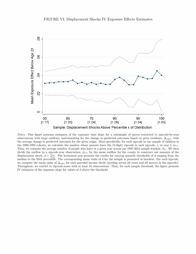
FIGURE VI: Displacement Shocks IV Exposure Eects Estimates

Notes: This figure presents estimates of the exposure time slope for a subsample of moves restricted to zipcode-by-yearobservations with large outflows, instrumenting for the change in predicted outcomes based on prior residents,

odps

, withthe average change in predicted outcomes for the given origin. More specifically, for each zipcode in our sample of children inthe 1980-1993 cohorts, we calculate the number whose parents leave the (5-digit) zipcode in each zipcode, z, in year t, m

zt

.Then, we compute the average number of people who leave in a given year across our 1997-2012 sample window, m

z

. We thendivide the outflow in a zipcode-year observation, m

zt

, by the mean outflow for the county to construct our measure of thedisplacement shock, d = mzt

mzt. The horizontal axis presents the results for varying quantile thresholds of d ranging from the

median to the 95th percentile. The corresponding mean value of d for the sample is presented in brackets. For each zipcode,we compute the mean value of

odps

for each parental income decile (pooling across all years and all movers in the zipcode).Throughout, we restrict to zipcode-years with at least 10 observations. Then, for each sample threshold, the figure presentsIV estimates of the exposure slope for values of d above the threshold.

FIGURE VII: Exposure Eects Based on Cross-Cohort Variation, with Cohort-Varying Intercepts

Notes: This figure presents estimates of the exposure time slope using own and placebo cohort place predictions. The sampleincludes all children in 1-time moving households whose parents moved when the child was less than or equal to 23 years old.The series in red traingles plots estimates of 9 separate regressions using place predictions for child in cohort c as if s/he werein cohort c + k, where k ranges between -4 and 4. By construction, the estimate for k = 0 corresponds to the baseline slope of0.040, illustrated in Figure IV (Panel B). Regressions include the predicted outcomes based on prior residents in the origin anddestination (for cohort c+k), and the interactions of the child’s age at the time of the move with the predicted outcomes in theorigin and destination based on prior residents (for cohort c + k). To be consistent with the baseline specifications, regressionsalso include dummy indicators for true cohort and its interaction with the predicted outcomes in the origin location. The blueseries reports coecients from a single regression that includes all variables in each of the regressions for k = ≠4, ..., 4 andplots the coecient on the interaction of the child’s age at the time of the move with the predicted outcome based on priorresidents in the destination location in cohort c + k.

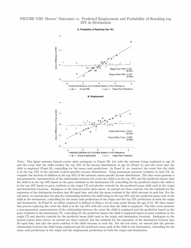
FIGURE VIII: Movers’ Outcomes vs. Predicted Employment and Probability of Reaching top10% in Destination

A. Probability of Reaching Top 10%

B. Employment

Notes: This figure presents binned scatter plots analogous to Figure III, but with the outcome being employed at age 24and the event that the child reaches the top 10% of the income distribution at age 24 (Panel A) and the event that thechild is employed (Panel B), controlling for the mean rank predictions. In Panel A, we construct the event that the childis in the top 10% of the national (cohort-specific) income distribution. Using permanent parental residents in each CZ, wecompute the fraction of children in the top 10% of the national cohort-specific income distribution. The blue series presents anon-parametric representation of the relationship between the event the child is in the top 10% and the predicted chance thatthe child is in the top 10% based on the prior residents in the destination CZ, controlling for the predicted chance the child isin the top 10% based on prior residents in the origin CZ and placebo controls for the predicted mean child rank in the originand destination locations. Analogous to the binned scatter plots above, we partial out these controls, bin the residuals for theregression of the destination location into 20 equal bins, and plot the mean residual of the child outcome in each bin. For thered series, we instead plot the placebo relationship between the child being in the top 10% and the predicted mean rank of thechild in the destination, controlling for the mean rank predictions in the origin and the top 10% predictions in both the originand destination. In Panel B, we define employed is defined as filing a w2 at some point during the age of 24. We then repeatthis process replacing the event the child is in the top 10% with the event that the child is employed. The blue series presentsa non-parametric representation of the relationship between the event the child is employed and the prediction based on theprior residents in the destination CZ, controlling for the predicted chance the child is employed based on prior residents in theorigin CZ and placebo controls for the predicted mean child rank in the origin and destination locations. Analogous to thebinned scatter plots above, we partial out these controls, bin the residuals for the regression of the destination location into20 equal bins, and plot the mean residual of the child outcome in each bin. For the red series, we instead plot the placeborelationship between the child being employed and the predicted mean rank of the child in the destination, controlling for themean rank predictions in the origin and the employment predictions in both the origin and destination.

FIGURE IX: Movers’ Outcomes vs. Gender-Specific Predicted Outcomes in Destination

Notes: This figures presents binned scatter plots analogous to Figure III, but using gender-specific predicted outcomes basedon prior residents. The blue series provides a non-parametric representation of the relationship between the child’s own genderplace prediction and the child’s outcome; the red series provides a non-parametric representation of the relationship betweenthe other (placebo) gender place predictions for the child’s outcome, controlling for the own gender prediction. The sampleincludes all children in 1-time moving households whose parents moved when the child was less than or equal to 13 yearsold. Child income is measured when the child is age 26. For the blue circle series, we regress the own gender destinationprediction for the child’s outcome on the other gender destination prediction, other gender origin prediction, and own genderorigin prediction. Similarly, we regress the child’s income rank on the other gender destination prediction, other genderorigin prediction, and own gender origin prediction. The figure then plots the relationship between these residuals fromthese regressions with sample means added to center the graphs. We construct 20 equal sized bins of the residuals from thedestination regression and, in each bin, plot mean of the residuals from the child rank regression. For the red series, we repeatthis process but using the placebo (other) gender predictions. We regress the other gender destination prediction for thechild’s outcome on the own gender destination prediction, other gender origin prediction, and own gender origin prediction.Similarly, we regress the child’s income rank on the own gender destination prediction, other gender origin prediction, andown gender origin prediction. The red triangle series then plots the relationship between these residuals from these regressionswith sample means added to center the graphs.

FIGURE X: Exposure Eect Estimates for College Attendence (18-23) and Marriage at Age 26

A. College Attendance (Age 18-23)

B. Marriage (Age 26)

Notes: This figure presents exposure eect estimates for college and marriage outcomes. In Panel A, we replicate the baselinespecification (equation 9) replacing the child’s outcomes with an indicator for college attendence at any age between 18-23.We construct separate analogous predicted outcomes based on the prior residents in each CZ for each outcome. We definecollege attendence as the existence of a 1098-T form (indicating college enrollment) when the child is 18-23 years old andrestrict the sample to observations we observe for years 18-23. Because we observe college attendance in years 1999-2012, weobtain estimates for ages at move of 8-29. In Panel B, we replicate the baseline specification (equation 9) replacing the child’soutcomes with an indicator for being married at age age 26 using the child’s filing status at age 26.

10

FIGURE XI: Exposure Eect Estimates for Teen Outcomes

A. Teen Employment at Age 16 B. Teen Employment at Age 17

C. Teen Employment at Age 18 D. Teenage birth

Notes: This figure presents exposure eect estimates for teen outcomes. Panels A-C replicate the baseline specification withorigin prediction controls (Figure IV, Panel B), but replaces the child’s outcomes with an indicator for working at age 16-18(defined as the existence of a W-2 during the year in which the child turned age a). Panel D presents estimates from thebaseline specification using teen birth as the outcome. We define teenage birth as having a birth in the calendar year prior toturning age 20 using birth certificate records from the social security administration’s death master file (DM-2), and estimatethe model separately for males and females.

11

FIGURE XII: The Geography of Exposure Eects on Income Across CZs

A. At 25th Percentile (µ25,c

)

B. At 75th Percentile (µ75,c

)

Notes: These figures present estimates of place eects, µpc

in for child income rank at age 26 by Commuting Zone, for childrenfrom families at the 25th percentile and 75th percentile of the parental income distribution. Section V discusses the estimationstrategy and sample restrictions. The values represent the causal eect of spending 1 additional year growing up in a CZ(relative to a population-weighted average CZ).

FIGURE XIII: Predicted Estimates: National CZ

A. At 25th Percentile (µ25,c

)

B. At 75th Percentile (µ75,c

)

Notes: These figures present forecast estimates of each CZ’s causal eects, µf

pc

, for below-median (p = 25) and above-median(p = 75) income families. We compute these forecasts using the methodology discussed in Section IX.A and, in particular,using the formula in Equation 21. For small-population CZs for which we do not have fixed eect estimates, we display thepermanent resident outcomes (which corresponds to the natural assumption that s

pc

= Πin Equation 21 in the case whenwe have no fixed eect estimate).

FIGURE XIV: Predicted Estimates for NY and Boston CSA by County

A. New York CSA, at 25th Percentile (µ25,c

) B. Boston CSA, at 25th Percentile (µ25,c

)

C. New York CSA, at 75th Percentile (µ75,c

) D. Boston CSA, at 75th Percentile (µ75,c

)

Notes: These figures present forecast estimates of the county-level causal eects, µf

pc

, for below-median (p = 25) and above-median (p = 75) income families in the New York and Boston Combined Statistical Areas (CSAs). We compute these using theformula in Equation 21 using the county-level fixed eect estimates, µ

pc

(which are the sum of the CZ and county-within-CZestimates, as discussed in Section XII.D), and the permanent resident forecasts, y

pc

, for each county.

FIGURE XV: Predictors of Exposure Eects For Children with Parents at 25th Percentile

A. At the Commuting Zone Level

B. At the County Level; within CZs

Notes: These figures show the coecients of regressions of the model components for below-median income families (p = 25)on a set of covariates analyzed in Chetty et al. (2014) which are normalized to have mean zero and unit standard deviation.The vertical line represents the coecient from a regression of the permanent resident outcomes, y25,c

, on the covariate.The solid bar represents the coecient from a regression of the causal component, T

c

µ25,c

, on the covariate, so that thedierence between the bar and the vertical line (denoted by the dashed horizontal line) represents the regression coecientfrom a regression of the sorting component, y25,c

≠ Tc

µ25,c

, on the covariate. The column on the far left divides the regressioncoecient by the standard deviation of µ25,c

, providing the implied correlation between the covariate and the causal eects. We

restrict the sample to CZs and counties for which we have both causal fixed eects and permanent resident outcome

measurements. The covariate definitions are provided in Appendix Table X. Results for additional covariates provided

in Tables XII-XV. Panel A presents the results at the CZ level. Panel B presents the results at the county within

CZ level by conditioning on CZ fixed eects.

FIGURE XVI: Predictors of Exposure Eects For Children with Parents at 75th Percentile

A. At the Commuting Zone Level

B. At the County Level; within CZs

Notes: These figures show the coecients of regressions of the model components for above-median income families (p = 75)on a set of covariates analyzed in Chetty et al. (2014) which are normalized to have mean zero and unit standard deviation.The vertical line represents the coecient from a regression of the permanent resident outcomes, y75,c

, on the covariate.The solid bar represents the coecient from a regression of the causal component, T

c

µ75,c

, on the covariate, so that thedierence between the bar and the vertical line (denoted by the dashed horizontal line) represents the regression coecientfrom a regression of the sorting component, y75,c

≠ Tc

µ75,c

, on the covariate. The column on the far left divides the regressioncoecient by the standard deviation of µ75,c

, providing the implied correlation between the covariate and the causal eects. We

restrict the sample to CZs and counties for which we have both causal fixed eects and permanent resident outcome

measurements. The covariate definitions are provided in Appendix Table X. Results for additional covariates provided

in Tables XII-XV. Panel A presents the results at the CZ level. Panel B presents the results at the county within

CZ level by conditioning on CZ fixed eects.

FIGURE XVII: Median Rent versus Exposure EectsA. Above-Median Segregated CZs with Populations above 100,000

B. Below-Median Segregated CZs with Populations above 100,000

C. CZs with Populations below 100,000

Notes: This figure presents binned scatterplots corresponding to a regression of median rent in the county (from the 2000Census) on the predicted exposure eect for that county at p = 25, µf

25,c

. In contrast to the model in Section IX, weconstruct the forecasts µf

25,c

using only the fixed eect estimates, µ25,c

normalized by their signal-to-total variance ratio (wedo not incorporate information from permanent residents, y

pc

, in order to avoid picking up correlations between prices andthe sorting components). Panels A-C present binned scatter plots of the relationship between median rent in the county andthe predicted exposure eect of the county, conditional on CZ fixed eects. We split counties into three groups: those inCZs with populations above and below 100,000 based on the 2000 Census. We then split the set of CZs with populationsabove 100,000 into two groups: those with above-median segregation/sprawl and below-median segregation/sprawl, wheresegregation/sprawl is defined by the fraction of people in the CZ that have commute times less than 15 minutes. Panel Areports the binned scatterplot for CZs with above-median segregation/sprawl and CZ populations above 100,000; Panel Breports the binned scatterplot for CZs with below-median segregation/sprawl and CZ populations above 100,000. Panel Creports the binned scatterplot for CZs with population below 100,000.

FIGURE XVIII: Median Rent versus Unobservable and Observable Exposure EectsA. Median Rent versus Observable Component

B. Median Rent versus Unobservable Component

Notes: This figure presents binned scatter plots corresponding to a regression of median rent on the observable and unobservablecomponents of the county-level forecasts, µf

25c

, on the sample of CZs with populations above 100,000, conditional on CZ fixedeects. We construct the observable component by regressing µ25,c

on five covariates that are standardized to have mean zeroand unit variance: the fraction of children with single parents, the fraction with travel time less than 15 minutes, the ginicoecient restricted to the 0-99th percentiles of the income distribution (which equals the gini minus the fraction of incomeaccruing to the top 1%), the fraction below the poverty line, and a residualized measure of test scores (see Appendix TableX for further variable details). We weight observations by the estimated precision of µ25,c

. We then define the “observable”component as the predicted values from this regression. For the unobservable component, we take the residual from thisregression and multiply it by its estimated total variance divided by the signal variance of the residual. The total variance isgiven by the variance of the residuals, weighted by the estimated precision of µ25,c

. To construct the signal variance of theresidual, we estimate the noise variance as the mean of the square of the standard errors, weighted by the estimated precisionof µ25,c

. Given the observable and unobservable components, Panel A presents the binned scatterplot corresponding to theregression of median rent on the observable component, controlling for CZ fixed eects and the unobservable component. Weregress median rent on the the unobservable component and CZ fixed eects and construct residuals. We then regress theobservable component on the unobservable component and CZ fixed eects and construct residuals. We bin these residualsof the observable component into vengtiles and within each vingtile plot the average of the median rent residuals. Hence, theslope of the line corresponds to the partial regression coecient of a regression of median rent on the observable component,controlling for the unobservable component and CZ fixed eects. For Panel B, we replace the observable and unobservablecomponents in the process for Panel A, so that the slope of the graph corresponds to the partial regression coecient on theunobservable component in a regression of median rent on the observable and unobservable components of the forecast.

ONLINE APPENDIX FIGURE I

Map of Boston CZ

Notes: This figure presents a county map of the Boston commuting zone.

ONLINE APPENDIX FIGURE II

Exposure Eect Estimates at Age 24, 26, 28, and 30

Notes: This figure replicates our baseline specification in equation (8), shown in Figure IVb, using incomes measured at age24, 26, 38, and 30. The figure presents estimates of b

m

for the specification in equation (6) that includes origin by parentincome decile by cohort by child age at move fixed eects. The figure reports the slopes from a regression of the b

m

coecientson m for m Æ 23, with standard errors in parentheses.

ONLINE APPENDIX FIGURE III

Exposure Eect Estimates using Parental Move as an Instrument for Child Exposure

Notes: This figure presents estimates of the coecients bm adjusted for the probability that the child follows the

parent to the destination. Formally, we construct the fraction of children who follow their parents when the parents

move when the child is m years old, „m, as the fraction of children who either (a) file a tax return in the destination,

(b) have a form W-2 mailing address in the destination location, or (c) attend a college (based on 1098-T filings

by institutions) in the destination location. The figure plots the series of bIVm =

bm≠”„m

+ ”, where ” = 0.125 is the

estimated selection eect shown in Figure IVa.

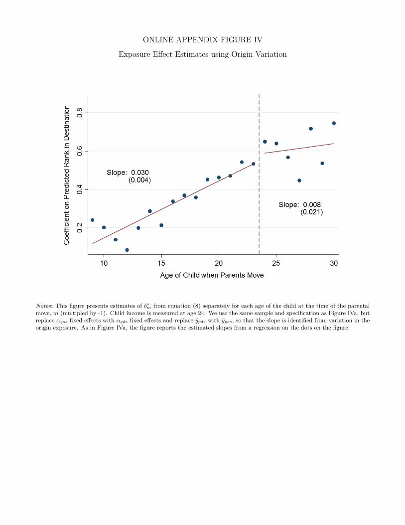
ONLINE APPENDIX FIGURE IV

Exposure Eect Estimates using Origin Variation

Notes: This figure presents estimates of bo

m

from equation (8) separately for each age of the child at the time of the parentalmove, m (multipled by -1). Child income is measured at age 24. We use the same sample and specification as Figure IVa, butreplace –

qos

fixed eects with –qds

fixed eects and replace ypds

with ypos

, so that the slope is identified from variation in theorigin exposure. As in Figure IVa, the figure reports the estimated slopes from a regression on the dots on the figure.

ONLINE APPENDIX FIGURE V

Map of Dierence in Gender Outcomes, ympcs ≠ yf

pcs, Evaluated at the 25th Percentile of ParentalIncome,

Notes: This figure presents estimates of the dierence in male versus famale outcomes of permanent residents, ympcs ≠ yf

pcs by

CZ, c, for income at age 24. To estimate ympcs and yf

pcs, we estimate linear regressions of child rank on parent income

rank for each CZ on separate male and female samples, pooling cohorts 1980-1988 cohorts.

ONLINE APPENDIX FIGURE VI

Predicted Income Rank at Age 30 - Permanent Residents

A. For Children with Parent at the 25thPercentile (CZ) B. For Children with Parent at the 75thPercentile (CZ)

C. For Children with Parent at the 25thPercentile (County) D. For Children with Parent at the 75thPercentile (County)

Notes: These figures present the estimated ypcs

by CZ and County for p = 25 and p = 75.

ONLINE APPENDIX FIGURE VII: Correlations of place eects by age (p25)

Notes: This figure presents the estimated correlation between ypc

across CZs when measured at age 32 with measurements atearlier ages (20-32). Correlations are weighted by CZ population in the 2000 Census. The vertical axis presents the estimatedcorrelation; the horizontal axis corresponds to the varying age of income measurement.

ONLINE APPENDIX FIGURE VIII: Distribution of Predicted Values by Gender

Notes: This figure presents the cumulative distribution of the gender-specific forecasts of county exposure eects for familyincome for children in below-median (p25) income families, µf

25,c

. The solid (blue) line presents the cumulative distributionfor male forecasts. The dashed (red) line presents the cumulative distribution of the female forecasts.

ONLINE APPENDIX FIGURE IX: Predicted Estimates: National CZ - Using Individual Incomes

A. At 25th Percentile (µ25,c

)

B. At 75th Percentile (µ75,c

)

Notes: These figures present forecast estimates of each CZ’s causal eects on individual income (as opposed to family income,shown in Figure XIII), µf

pc

, for below-median (p = 25) and above-median (p = 75) income families. We estimate the fixedeects, µ

pc

, and permanent resident outcomes, ypc

, using the child’s individual income at age 26. We then compute theseforecasts using the methodology discussed in Section IX.A and, in particular, using the formula in Equation 21. For small-population CZs for which we do not have fixed eect estimates, we display the permanent resident outcomes (which correspondsto the natural assumption that s

pc

= Πin Equation 21 in the case when we have no fixed eect estimate).

ONLINE APPENDIX FIGURE X: Predicted Estimates: National CZ - Male and Female

A. Male (µ25,c

)

B. Female (µ25,c

)

Notes: These figures present forecast estimates of each CZ’s causal eects on family income for children in below-median(p = 25) families on separate samples of male (Panel A) and female (Panel B) children. We estimate the fixed eects, µ

pc

, andpermanent resident outcomes, y

pc

, using the child’s family income at age 26 on separate gender samples. We then computethese forecasts using the methodology discussed in Section IX.A and, in particular, using the formula in Equation 21. Forsmall-population CZs for which we do not have fixed eect estimates, we display the permanent resident outcomes (whichcorresponds to the natural assumption that s

pc

= Πin Equation 21 in the case when we have no fixed eect estimate).

ONLINE APPENDIX FIGURE XI: Predicted Estimates: National CZ - Male and Female - UsingIndividual Incomes

A. Male (µ25,c

)

B. Female (µ25,c

)

Notes: These figures present forecast estimates of each CZ’s causal eects on individual income for children in below-median(p = 25) families on separate samples of male (Panel A) and female (Panel B) children. We estimate the fixed eects, µ

pc

,and permanent resident outcomes, y

pc

, using the child’s individual income at age 26 on separate gender samples. We thencompute these forecasts using the methodology discussed in Section IX.A and, in particular, using the formula in Equation 21.For small-population CZs for which we do not have fixed eect estimates, we display the permanent resident outcomes (whichcorresponds to the natural assumption that s

pc

= Πin Equation 21 in the case when we have no fixed eect estimate).

Variable Mean Std. Dev. Median Sample Size(1) (2) (3) (4)

Non-MoversParent Income 79,802 310,537 52,800 44,175,313Child family income at 24 24,853 130,276 19,700 22,933,771Child family income at 26 33,706 149,981 26,200 17,592,224Child family income at 30 48,377 129,801 35,400 7,239,831Child individual earnings at 24 20,484 193,368 17,000 23,046,067College attendence (18-23) 0.69 0.46 1.00 23,526,466College quality (18-23) 31,306 13,138 30,900 23,526,466Teen Birth (13-19) 0.11 0.31 0.00 16,829,532Teen employment at age 16 0.28 0.45 0.00 43,950,854

Number of movers1 time 7,784,9762 times 4,725,8433 times 2,010,5374+ times 2,043,889Total 16,565,245

1 time -3 times MoversParent Income 71,422 285,880 44,100 14,521,356Child family income at 24 23,484 62,130 18,200 6,810,190Child family income at 26 31,249 90,855 23,700 5,127,832Child family income at 30 44,812 133,057 32,200 2,059,365Child individual earnings at 24 18,804 54,408 15,200 6,810,190College attendence (18-23) 0.636 0.481 1.000 7,067,553College quality (18-23) 29,386 12,537 28,700 7,067,553Teen Birth (13-19) 0.137 0.344 0.000 5,225,131Teen employment at age 16 0.268 0.443 0.000 14,521,356

One-time MoversParent Income 85,271 316,143 48,500 3,418,710Child family income at 24 23,867 56,564 18,700 1,553,021Child family income at 26 32,419 108,431 24,300 1,160,278Child family income at 30 47,882 117,450 33,200 460,457Child individual earnings at 24 19,781 48,784 16,200 1,553,021College attendence (18-23) 0.695 0.460 1.000 1,622,145College quality (18-23) 31,332 13,430 30,600 1,622,145Teen Birth (13-19) 0.109 0.311 0.000 1,212,352Teen employment at age 16 0.257 0.437 0.000 3,418,710

TABLE ISummary Statistics for CZ Permanent Residents and Movers

Notes: The table presents summary statistics for the samples used in the CZ-level analyses. We split the summarystatistics into the permanent residents ("non-movers") whose parents do not move across CZs throughout our samplewindow (1996-2012) and movers. Section III provides details on variable and sample definitions.

(1) (2) (3) (4) (5) (6) (7) (8a) (8b) (8c) (9) (10)

Exposure Slope 0.040 0.041 0.041 0.031 0.036 0.041 0.031 0.040 0.037 0.031 0.039 0.040(0.002) (0.002) (0.006) (0.005) (0.002) (0.002) (0.002) (0.001) (0.004) (0.006) (0.001) (0.002)

ControlsCohort-Varying Intercept X X X X X X X X X XChild age (m) x yops

Interactions X

Child Income Definition Family Family Family Family Family Family Family Family Family Family Family Individual

Num of Obs. 1,553,021 1,287,773 687,323 604,602 1,553,021 1,553,021 1,473,218 4,374,418 4,374,418 4,374,418 4,374,418 1,553,021

Pooled ConstrainedIndividual Income

Origin Controls

(Destination)

No Cohort Controls

Claimed Sample

TABLE IIExposure Effect Estimates

Notes: Table II reports the coefficients on the child's age at the time of the parental move interacted with the difference in the predicted outcomes based on prior residents in the destination relative tothe origin. Coefficients are multipled by -1 to correspond to exposure to destination. We allow separate lines allowed for child age <= 23 and child age > 23 at the time of the parental move. Column (1)reports the coefficient β in equation (9). Column (2) restricts the sample to those below age 23 at the time of the move. Column (3) restricts the sample to those below age 18. Column (4) further restrictsto the sample of children who are claimed as a dependent on a 1040 in the destination CZ in the years subsequent to the move. Column (5) drops the cohort interactions with the predicted outcomes ofpermanent residents in the origin and destination location and instead includes one control for the predicted outcomes of those in the origin location. Column (6) adds controls for the child's age at moveinteracted with the predicted outcomes of those in the origin location to the baseline specification in column (1) and equation (9). Column (7) adds the child's CZ in adulthood (2012) as a fixed effect.Column (8a-c) present estimates for the exposure effect of the 1st, 2nd, and 3rd move using the sample of 1-3-time movers, as opposed to the 1-time movers sample. Column (9) presents the estimatesof the exposure effect restricting the coefficient to be the same across each move. Column (10) presents the baseline specification (equation 9) using individual income for both the outcome andpredicted outcomes in the origin and destination

Specification:

Pooled movesBaseline Spec.1st

Destination

Child CZ Fixed

Effects2nd

Destination3rd

DestinationAge ≤ 18Age ≤ 23

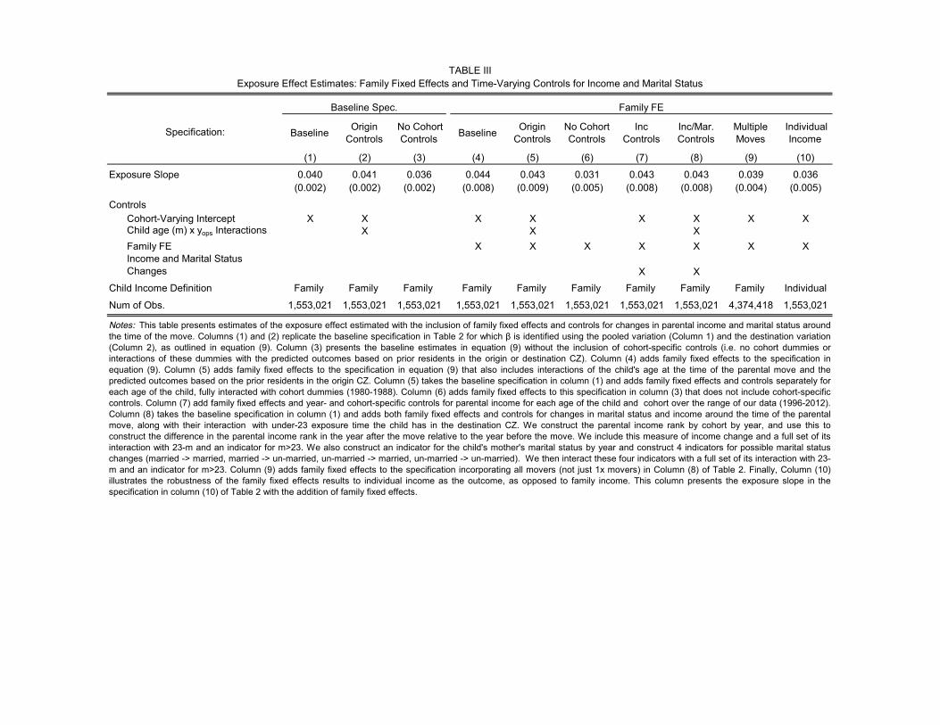
Baseline Origin Controls

No Cohort Controls Baseline Origin

ControlsNo Cohort Controls

Inc Controls

Inc/Mar. Controls

Multiple Moves

Individual Income

(1) (2) (3) (4) (5) (6) (7) (8) (9) (10)

Exposure Slope 0.040 0.041 0.036 0.044 0.043 0.031 0.043 0.043 0.039 0.036(0.002) (0.002) (0.002) (0.008) (0.009) (0.005) (0.008) (0.008) (0.004) (0.005)

ControlsCohort-Varying Intercept X X X X X X X XChild age (m) x yops Interactions X X XFamily FE X X X X X X XIncome and Marital Status Changes X X

Child Income Definition Family Family Family Family Family Family Family Family Family Individual

Num of Obs. 1,553,021 1,553,021 1,553,021 1,553,021 1,553,021 1,553,021 1,553,021 1,553,021 4,374,418 1,553,021

Notes: This table presents estimates of the exposure effect estimated with the inclusion of family fixed effects and controls for changes in parental income and marital status aroundthe time of the move. Columns (1) and (2) replicate the baseline specification in Table 2 for which β is identified using the pooled variation (Column 1) and the destination variation(Column 2), as outlined in equation (9). Column (3) presents the baseline estimates in equation (9) without the inclusion of cohort-specific controls (i.e. no cohort dummies orinteractions of these dummies with the predicted outcomes based on prior residents in the origin or destination CZ). Column (4) adds family fixed effects to the specification inequation (9). Column (5) adds family fixed effects to the specification in equation (9) that also includes interactions of the child's age at the time of the parental move and thepredicted outcomes based on the prior residents in the origin CZ. Column (5) takes the baseline specification in column (1) and adds family fixed effects and controls separately foreach age of the child, fully interacted with cohort dummies (1980-1988). Column (6) adds family fixed effects to this specification in column (3) that does not include cohort-specificcontrols. Column (7) add family fixed effects and year- and cohort-specific controls for parental income for each age of the child and cohort over the range of our data (1996-2012).Column (8) takes the baseline specification in column (1) and adds both family fixed effects and controls for changes in marital status and income around the time of the parentalmove, along with their interaction with under-23 exposure time the child has in the destination CZ. We construct the parental income rank by cohort by year, and use this toconstruct the difference in the parental income rank in the year after the move relative to the year before the move. We include this measure of income change and a full set of itsinteraction with 23-m and an indicator for m>23. We also construct an indicator for the child's mother's marital status by year and construct 4 indicators for possible marital statuschanges (married -> married, married -> un-married, un-married -> married, un-married -> un-married). We then interact these four indicators with a full set of its interaction with 23-m and an indicator for m>23. Column (9) adds family fixed effects to the specification incorporating all movers (not just 1x movers) in Column (8) of Table 2. Finally, Column (10)illustrates the robustness of the family fixed effects results to individual income as the outcome, as opposed to family income. This column presents the exposure slope in thespecification in column (10) of Table 2 with the addition of family fixed effects.

TABLE IIIExposure Effect Estimates: Family Fixed Effects and Time-Varying Controls for Income and Marital Status

Specification:

Baseline Spec. Family FE

(1) (2) (3) (4) (5) (6)

0.043 0.040 0.046 0.045(0.002) (0.003) (0.003) (0.004)

0.022 0.004 0.021 0.000(0.002) (0.003) (0.002) (0.003)

Num. of Obs. 1,553,021 1,553,021 1,553,021 1,553,021 1,553,021 1,553,021

TABLE IVDistributional Convergence

Child Rank in top 10% Child Employed

Notes: Table presents estimates of the exposure time relationships for the outcome of being in the top 10% of thecohort-specific income distribution at age 24 and being employed. We define employment as an indicator for filinga W-2 at some point during the year in which the child is age 24. Analogous to these outcomes, we constructpredicted outcomes using permenent residents each CZ. Column (1) presents the estimated exposure time slopeusing top 10% indicator as the dependent variable and predicted outcomes based on permanent residents in theorigin and destination CZ. Column (2) continues to use the indicator of being in the top 10% as the dependentvariable, but uses the mean rank predictions from the baseline regressions as the origin and destinationpredictions. Column (3) combines all variables in specifications (1) and (2). Column (4) presents the estimatedexposure time slope using an indicator of being employed as the dependent variable and predicted outcomesbased on permanent residents in the origin and destination CZ. Column (5) retains the employment indicator asthe dependent variable but replaces the predicted outcomes in the origin and destination with the mean rankpredictions from the baseline regressions. Column (6) combines all variables in specifications (4) and (5).

Mean Rank Prediction (Placebo)

Distributional Prediction

(1) (2) (3) (4) (5) (6) (7)0.038 0.031 0.031 0.027 0.0308

(0.002) (0.003) (0.006) (0.006) (0.007)

0.034 0.009 0.017 0.017 0.0116(0.002) (0.003) (0.006) (0.006) (0.007)

Family Fixed Effects X X X X

Sample 2-Gender HH

Num. of Obs. 1,552,898 1,552,898 1,552,898 1,552,898 1,552,898 1,552,898 490964

TABLE VGender Placebos

Notes: Table presents estimates of the exposure time relationships using gender-specific predictions based on prior residents.The outcome is child rank when the child is 24 years old. Column (1) presents estimates for the baseline specification replacingthe predicted outcomes based on prior residents in the origin and destination with gender-specific predictions. Column (2)replaces own-gender predicted outcomes with predicted outcomes in the origin and destination based on the other gender.Column (3) combines all variables in the specification in (1) and (2). Columns (4)-(6) repeat the specifications in (1)-(3) with theaddition of family fixed effects. Column (7) repeats the specification in (6) but restricts to households with at least two childrenand at least one of each gender.

No Family Fixed Effects

Full Sample Full Sample

Family Fixed Effects

Other Gender Prediction (Placebo)

Own Gender Prediction

(1) (2) (3) (4) (5) (6) (7)

Exposure Slope 0.035 0.033 0.022 0.032 0.027 0.029 0.024(0.003) (0.011) (0.003) (0.004) (0.003) (0.025) (0.002)

Num of Obs. 654,491 654,491 617,502 457,140 2,900,311 2,900,311 7,311,431

Notes: Table II reports exposure effect coefficients in equation (9), analogous to those presented in Tables II andIII, using county-level predictions for the sample of 1-time county movers. Column (1) presents the baselinespecification analogous to Column (1) of Table 2, replacing CZ-level predictions with county-level predictionsbased on prior residents. We restrict the sample to moves of at least 100 miles and require the county-levelpopulation to be at least 250,000 in the origin and destination county. Column (2) adds family fixed effects to thespecification in Column (1). Columns (3)-(7) drop the distance restriction and consider the set of within-CZ countymoves (between counties with populations of at least 250,000). Column (3) replicates the baseline specification.Column (4) replicates the baseline specification using income at age 26 as the outcome, analogous to theoutcomes considered in Section V. Column (5) presents the pooled estimate that stacks all outcomes for ages 24and above (multiple observations per person). Column (6) adds family-by-age of outcome fixed effects to thespecification in Column (5). Column (7) expands the sample in Column (5) to include moves between all CZs withpopulations above 10,000).

Table VICounty Exposure Effect Estimates

Specification:

Baseline Spec. Within CZ Moves

Baseline Family FE Age 24 Age 26 Small CZsFamily FEAge ≥ 24

Below Median (p25)

Above Median (p75)

Below Median (p25)

Above Median (p75)

Below Median (p25)

Above Median (p75)

Model Component (1) (2) (3) (4) (5) (6)

Signal vs. Noise (per year of exposure)Raw (per year) Exposure Effect (SD) 0.248 0.243 0.434 0.435 0.357 0.361Noise (SD) 0.210 0.218 0.402 0.407 0.343 0.344Signal of Exposure Effects (SD) 0.132 0.107 0.165 0.155 0.099 0.112Signal to Noise Ratio 0.398 0.241 0.170 0.144 0.084 0.106

Correlation between p25 and p75 Exposure Effects

Sorting vs. Causal Components (TC=20 yrs)Causal Effect (SD of Signal) 2.647 2.139 3.308 3.092 1.984 2.233Permanent Residents (SD) 3.259 2.585 4.203 3.257 2.653 1.982Sorting Component (SD) 1.960 1.097 3.033 3.203 2.315 3.009Correlation between Sorting and Causal Effect -0.021 0.193 -0.123 -0.465 -0.246 -0.753

Notes: This table presents the estimated variance components of the fixed effects model in equation (16). Panel A presents the estimates of the raw variance of theestimates. The first row presents the raw standard deviation across CZs, weighting by precision (1/SE, where SE is the estimated standard error of the estimate). Thesecond row presents the estimated standard deviation of the sampling noise (again weighted by precision, 1/SE). The third row presents the estimated signal standarddeviation, computed using the formula Signal_Variance = Total Variance - Noise Variance. The fourth row presents the signal to noise ratio (=Signal Variance / NoiseVariance). The last row of panel A presents the correlation between the 25th and 75th percentile estimates. To construct this correlation, we compute the covariance using asplit sample of above-median and below-median samples to estimate the p75 and p25 estimates, respectively, to avoid mechanical correlations, and then divide by thestandard deviations of the p25 and p75 place effects (estimated on these split samples) to arrive at an estimate of the correlation. Panel B presents the model variancecomponents. The first row presents the standard deviation of the causal effects (=20*signal of exposure effects). The second row presents the standard deviation of thepermanent resident outcomes (precision weighted). The third row presents the standard deviation of the sorting component (precision weighted). See the text for details oncomputing this standard deviation. The fourth row presents the estimated correlation between the sorting and causal effect across CZs. The columns present the estimateson various samples. Columns (1)-(2) present the estimates for below-median and above-median income families across Commuting Zones; Columns (3)-(4) present theestimates across counties. Columns (5)-(6) present the implied estimates for counties within CZs. For example, we compute the standard deviations using the identity:var(county_within_cz) = var(county) - var(cz).

Table VII

County within CZ

Panel B: Model Variance Components

Panel A: Exposure Effect Estimates

Model Variance Components: Causal and Selection Effects

Commuting Zones Counties

0.724 0.287 0.080

Prediction RMSE $ Increase % Increase Prediction RMSE $ Increase % Increase(1) (2) (3) (4) (5) (6) (7) (8)

Salt Lake City UT 0.166 0.066 135.9 0.521 0.105 0.041 88.4 0.218 (1)Seattle WA 0.140 0.059 114.3 0.438 -0.009 0.038 -7.3 -0.018 (2)Washington DC DC 0.105 0.051 85.8 0.329 0.062 0.034 51.7 0.127 (3)Minneapolis MN 0.103 0.065 84.1 0.322 0.077 0.041 65.0 0.160 (4)Fort Worth TX 0.057 0.061 46.6 0.178 0.049 0.039 41.3 0.102 (5)San Diego CA 0.056 0.054 46.1 0.177 -0.131 0.038 -110.0 -0.271 (6)Boston MA 0.055 0.061 45.3 0.174 0.033 0.040 27.7 0.068 (7)Manchester NH 0.051 0.070 41.8 0.160 0.025 0.041 20.7 0.051 (8)San Jose CA 0.048 0.065 39.1 0.150 -0.118 0.039 -99.2 -0.244 (9)Las Vegas NV 0.043 0.057 35.0 0.134 -0.078 0.039 -65.6 -0.162 (10)Denver CO 0.042 0.065 34.0 0.130 -0.060 0.038 -50.5 -0.124 (11)Portland OR 0.038 0.067 31.0 0.119 -0.091 0.041 -76.4 -0.188 (12)San Francisco CA 0.029 0.060 23.4 0.090 -0.119 0.037 -99.6 -0.245 (13)Pittsburgh PA 0.013 0.065 10.8 0.041 0.104 0.041 87.6 0.216 (14)Newark NJ 0.012 0.051 9.5 0.036 0.057 0.034 48.2 0.119 (15)Providence RI 0.007 0.067 5.7 0.022 0.022 0.042 18.4 0.045 (16)Sacramento CA 0.006 0.058 4.6 0.018 -0.144 0.038 -120.6 -0.297 (17)Phoenix AZ 0.004 0.049 3.1 0.012 -0.018 0.038 -15.1 -0.037 (18)Buffalo NY -0.003 0.067 -2.2 -0.009 0.010 0.041 8.6 0.021 (19)Kansas City MO -0.007 0.067 -5.4 -0.021 0.020 0.042 16.7 0.041 (20)Houston TX -0.025 0.050 -20.7 -0.079 0.006 0.036 5.3 0.013 (21)Miami FL -0.026 0.044 -20.9 -0.080 -0.201 0.039 -169.0 -0.416 (22)Philadelphia PA -0.029 0.057 -23.5 -0.090 0.005 0.037 3.9 0.010 (23)Grand Rapids MI -0.031 0.070 -25.7 -0.098 0.066 0.043 55.6 0.137 (24)Dallas TX -0.038 0.055 -30.8 -0.118 -0.009 0.036 -7.8 -0.019 (25)Cleveland OH -0.042 0.062 -34.7 -0.133 -0.025 0.041 -21.1 -0.052 (26)Bridgeport CT -0.045 0.059 -37.2 -0.143 0.028 0.038 23.6 0.058 (27)Jacksonville FL -0.048 0.061 -39.0 -0.149 -0.071 0.042 -59.6 -0.147 (28)Milwaukee WI -0.048 0.067 -39.3 -0.150 0.044 0.042 37.1 0.091 (29)Dayton OH -0.062 0.071 -51.1 -0.196 0.015 0.043 12.9 0.032 (30)Cincinnati OH -0.082 0.069 -67.3 -0.258 0.063 0.041 53.1 0.131 (31)Columbus OH -0.086 0.068 -70.7 -0.271 0.006 0.042 5.3 0.013 (32)Nashville TN -0.087 0.070 -71.4 -0.274 -0.027 0.042 -22.6 -0.056 (33)St. Louis MO -0.090 0.067 -73.7 -0.282 0.029 0.041 24.6 0.061 (34)Austin TX -0.097 0.066 -79.6 -0.305 -0.098 0.040 -82.6 -0.203 (35)Baltimore MD -0.103 0.066 -84.1 -0.322 0.067 0.039 56.4 0.139 (36)San Antonio TX -0.110 0.063 -90.1 -0.345 -0.078 0.040 -65.2 -0.160 (37)Tampa FL -0.114 0.048 -92.8 -0.356 -0.128 0.040 -107.8 -0.265 (38)New York NY -0.117 0.039 -95.5 -0.366 -0.032 0.035 -26.7 -0.066 (39)Indianapolis IN -0.118 0.070 -96.9 -0.371 -0.019 0.041 -16.3 -0.040 (40)Atlanta GA -0.124 0.043 -101.3 -0.388 -0.094 0.036 -78.7 -0.194 (41)Los Angeles CA -0.130 0.038 -105.9 -0.406 -0.226 0.032 -189.4 -0.466 (42)Detroit MI -0.136 0.054 -111.0 -0.425 -0.125 0.039 -105.3 -0.259 (43)Orlando FL -0.136 0.054 -111.3 -0.427 -0.137 0.040 -115.1 -0.284 (44)Chicago IL -0.154 0.048 -126.2 -0.484 -0.035 0.033 -29.1 -0.072 (45)Fresno CA -0.164 0.062 -134.3 -0.515 -0.120 0.042 -100.6 -0.248 (46)Port St. Lucie FL -0.174 0.057 -142.6 -0.547 -0.198 0.040 -166.7 -0.410 (47)Raleigh NC -0.195 0.065 -159.3 -0.610 -0.114 0.041 -96.0 -0.236 (48)Charlotte NC -0.205 0.061 -167.6 -0.642 -0.084 0.040 -70.7 -0.174 (49)New Orleans LA -0.214 0.065 -175.3 -0.672 -0.060 0.042 -50.1 -0.123 (50)

Row Number

Notes: Table presents per-year exposure predictions for the 50 largest CZs using the estimation strategy discussed in Section VIII. Column (1) reportsthe predictions for the child's family income rank at age 26. Column (2) reports the root mean square error for this prediction, computed as the squareroot of 1/(1/v_r + 1/v)) where v_r is the residual signal variance and v is the squared standard error of the fixed effect estimate. Column (3) scales thenumbers to dollars by multiplying the estimates in column (1) by 818, the coefficient obtained by regressing the permanent resident outcomes at p25for child family income at age 26 on the analogous outcomes for child rank at age 26. Column (4) divides the income impacts in column (3) by themean income of children from below-median (p25) income families of $26,090. Columns (5)-(8) report the analogous statistics for above-medianincome families. Column (5) reports the prediction for the child's family income rank at age 26; column (6) reports the root mean square error. Column(7) scales the numbers in Column (1) by 2.068, the coefficient obtained by regressing the permanent resident outcomes at p25 for child family incomeat age 26 on the analogous outcomes for child rank at age 26. Column (8) divides the income impacts on column (5) by the mean income of childrenfrom above-median (p75) income families of 40,601.

Predicted Place Effects for 50 Largest CZsTable VIII

Below-Median Income Parents (p25) Above-Median Income Parents (p75)Scaling ScalingFamily Income RankFamily Income Rank

Commuting ZoneState

Prediction RMSE $ Increase % Increase Prediction RMSE $ Increase % IncreaseCounty State (1) (2) (3) (4) (5) (6) (7) (8)

Dupage IL 0.255 0.090 208.8 0.800 0.076 0.077 63.8 0.157 (1)Fairfax VA 0.239 0.100 195.5 0.749 0.265 0.096 222.5 0.548 (2)Snohomish WA 0.224 0.099 182.9 0.701 0.058 0.094 48.9 0.120 (3)Bergen NJ 0.220 0.102 179.7 0.689 0.152 0.099 127.7 0.315 (4)Bucks PA 0.198 0.101 161.6 0.620 -0.023 0.098 -19.3 -0.047 (5)Norfolk MA 0.183 0.101 149.6 0.573 0.151 0.099 126.5 0.312 (6)Montgomery PA 0.155 0.096 127.0 0.487 0.072 0.092 60.5 0.149 (7)Montgomery MD 0.151 0.099 123.5 0.473 0.003 0.098 2.2 0.005 (8)King WA 0.149 0.084 121.8 0.467 0.077 0.076 64.8 0.160 (9)Middlesex NJ 0.146 0.102 119.1 0.456 0.013 0.101 11.2 0.027 (10)Contra Costa CA 0.141 0.095 115.2 0.442 -0.069 0.091 -58.3 -0.144 (11)Middlesex MA 0.123 0.091 100.6 0.386 0.013 0.089 11.0 0.027 (12)Macomb MI 0.111 0.088 91.1 0.349 0.028 0.091 23.1 0.057 (13)Salt Lake UT 0.099 0.095 80.7 0.309 0.016 0.093 13.8 0.034 (14)Ventura CA 0.099 0.100 80.6 0.309 -0.055 0.093 -46.0 -0.113 (15)San Mateo CA 0.085 0.102 69.2 0.265 -0.035 0.102 -29.7 -0.073 (16)Worcester MA 0.075 0.107 61.4 0.235 0.130 0.107 109.3 0.269 (17)Monmouth NJ 0.075 0.103 61.2 0.235 0.073 0.096 61.7 0.152 (18)Honolulu HI 0.073 0.100 59.9 0.230 -0.130 0.113 -109.2 -0.269 (19)Hudson NJ 0.066 0.101 54.4 0.208 0.161 0.110 135.5 0.334 (20)Kern CA 0.062 0.086 50.4 0.193 -0.059 0.110 -49.9 -0.123 (21)Clark NV 0.059 0.074 48.3 0.185 -0.046 0.087 -38.9 -0.096 (22)San Diego CA 0.058 0.063 47.8 0.183 -0.136 0.064 -114.4 -0.282 (23)Providence RI 0.048 0.101 39.2 0.150 -0.043 0.108 -35.8 -0.088 (24)San Francisco CA 0.045 0.100 37.1 0.142 -0.183 0.104 -154.0 -0.379 (25)

Jefferson KY -0.137 0.105 -112.3 -0.431 0.022 0.111 18.5 0.046 (75)Franklin OH -0.137 0.092 -112.4 -0.431 0.114 0.096 95.9 0.236 (76)San Bernardino CA -0.140 0.062 -114.5 -0.439 -0.245 0.073 -205.9 -0.507 (77)Davidson TN -0.141 0.098 -115.6 -0.443 -0.036 0.105 -29.8 -0.073 (78)Pima AZ -0.142 0.083 -116.5 -0.446 -0.139 0.099 -116.7 -0.287 (79)Montgomery OH -0.142 0.104 -116.5 -0.447 -0.016 0.116 -13.2 -0.032 (80)Travis TX -0.147 0.089 -120.2 -0.461 -0.159 0.087 -133.6 -0.329 (81)Essex NJ -0.147 0.096 -120.5 -0.462 0.074 0.098 61.8 0.152 (82)Bexar TX -0.152 0.090 -124.7 -0.478 -0.092 0.122 -77.4 -0.191 (83)Milwaukee WI -0.158 0.096 -129.4 -0.496 -0.027 0.097 -22.4 -0.055 (84)Riverside CA -0.161 0.067 -131.6 -0.505 -0.248 0.075 -208.3 -0.513 (85)Los Angeles CA -0.164 0.045 -134.1 -0.514 -0.254 0.049 -212.9 -0.524 (86)Wake NC -0.171 0.101 -139.8 -0.536 -0.094 0.102 -79.1 -0.195 (87)New York NY -0.173 0.076 -141.5 -0.542 -0.275 0.100 -230.7 -0.568 (88)Fulton GA -0.173 0.077 -141.6 -0.543 0.024 0.083 19.9 0.049 (89)Bronx NY -0.174 0.076 -142.0 -0.544 -0.201 0.107 -169.1 -0.416 (90)Wayne MI -0.182 0.077 -148.6 -0.570 -0.073 0.079 -61.5 -0.152 (91)Orange FL -0.193 0.077 -157.9 -0.605 -0.093 0.092 -77.9 -0.192 (92)Cook IL -0.204 0.060 -166.9 -0.640 -0.030 0.051 -24.9 -0.061 (93)Palm Beach FL -0.208 0.084 -169.8 -0.651 -0.314 0.097 -263.9 -0.650 (94)Marion IN -0.209 0.097 -170.8 -0.655 -0.102 0.091 -85.4 -0.210 (95)Shelby TN -0.210 0.093 -171.5 -0.657 0.030 0.103 25.2 0.062 (96)Fresno CA -0.215 0.089 -176.1 -0.675 -0.051 0.110 -42.4 -0.105 (97)Hillsborough FL -0.220 0.088 -180.3 -0.691 -0.192 0.102 -161.4 -0.397 (98)Baltimore City MD -0.223 0.092 -182.4 -0.699 -0.017 0.097 -14.6 -0.036 (99)Mecklenburg NC -0.231 0.095 -188.6 -0.723 -0.090 0.100 -75.5 -0.186 (100)

Row Number

Notes: Table presents per-year exposure predictions for the top 25 and bottom 25 largest counties using the estimation strategy discussed inSection VIII, sorted by the impact on family income rank for children in below-median (p25) income families. Column (1) reports the predictions forthe child's family income rank at age 26. Column (2) reports the root mean square error for this prediction, computed as the square root of 1/(1/v_r+ 1/v)) where v_r is the residual signal variance and v is the squared standard error of the fixed effect estimate. Column (3) scales the numbers todollars by multiplying by the estimates in column (1) by 3.13, the coefficient obtained by regressing the permanent resident outcomes at p25 forchild family income at age 26 on the analogous outcomes for child rank at age 26. Column (4) divides the income impacts in column (3) by themean income of children from below-median (p25) income families of $26,090. Columns (5)-(8) report the analogous statistics for above-medianincome families. Column (5) reports the prediction for the child's family income rank at age 26; column (6) reports the root mean square error.Column (7) scales the numbers in Column (1) by 2.068, the coefficient obtained by regressing the permanent resident outcomes at p25 for childfamily income at age 26 on the analogous outcomes for child rank at age 26. Column (8) divides the income impacts on column (5) by the meanincome of children from above-median (p75) income families of 40,601.

Table IXPredicted Place Effects for 100 Largest Counties (Top and Bottom 25)

Family Income RankBelow-Median Income Parents (p25) Above-Median Income Parents (p75)

Scaling ScalingFamily Income Rank

Prediction RMSE % Increase Prediction RMSE % Increase Prediction RMSE % Increase Prediction RMSE % Increase(1) (2) (3) (4) (5) (6) (7) (8) (9) (10) (11) (12)

Seattle WA 0.154 0.101 0.457 0.217 0.087 0.711 0.140 0.059 0.438 0.185 0.067 0.581 (1)Minneapolis MN 0.155 0.130 0.461 0.154 0.101 0.503 0.103 0.065 0.322 0.154 0.082 0.484 (2)Salt Lake City UT 0.060 0.131 0.178 0.234 0.105 0.767 0.166 0.066 0.521 0.147 0.084 0.461 (3)Washington DC DC 0.078 0.097 0.233 0.108 0.081 0.353 0.105 0.051 0.329 0.093 0.063 0.292 (4)Portland OR 0.127 0.124 0.379 0.040 0.100 0.131 0.038 0.067 0.119 0.084 0.079 0.262 (5)Fort Worth TX 0.097 0.109 0.290 0.021 0.090 0.069 0.057 0.061 0.178 0.059 0.071 0.186 (6)Las Vegas NV -0.029 0.091 -0.087 0.147 0.078 0.482 0.043 0.057 0.134 0.059 0.060 0.185 (7)San Diego CA 0.019 0.098 0.056 0.087 0.084 0.286 0.056 0.054 0.177 0.053 0.064 0.167 (8)San Francisco CA -0.005 0.101 -0.014 0.086 0.085 0.281 0.029 0.060 0.090 0.041 0.066 0.127 (9)Pittsburgh PA -0.002 0.132 -0.005 0.070 0.102 0.230 0.013 0.065 0.041 0.034 0.084 0.107 (10)Boston MA 0.055 0.106 0.163 0.012 0.089 0.039 0.055 0.061 0.174 0.033 0.069 0.105 (11)San Jose CA -0.127 0.114 -0.378 0.189 0.093 0.618 0.048 0.065 0.150 0.031 0.073 0.096 (12)Manchester NH 0.063 0.137 0.187 -0.011 0.106 -0.036 0.051 0.070 0.160 0.026 0.086 0.081 (13)Denver CO 0.035 0.116 0.104 0.008 0.095 0.026 0.042 0.065 0.130 0.021 0.075 0.067 (14)Phoenix AZ -0.054 0.084 -0.161 0.076 0.075 0.250 0.004 0.049 0.012 0.011 0.056 0.035 (15)Cleveland OH 0.096 0.121 0.284 -0.078 0.099 -0.256 -0.042 0.062 -0.133 0.009 0.078 0.027 (16)Sacramento CA -0.076 0.100 -0.227 0.069 0.085 0.228 0.006 0.058 0.018 -0.003 0.066 -0.011 (17)Providence RI -0.001 0.131 -0.004 -0.007 0.103 -0.023 0.007 0.067 0.022 -0.004 0.083 -0.013 (18)Newark NJ 0.039 0.084 0.116 -0.048 0.072 -0.158 0.012 0.051 0.036 -0.004 0.056 -0.014 (19)Buffalo NY -0.008 0.124 -0.024 -0.007 0.099 -0.022 -0.003 0.067 -0.009 -0.007 0.079 -0.023 (20)Grand Rapids MI 0.003 0.144 0.009 -0.049 0.109 -0.161 -0.031 0.070 -0.098 -0.023 0.090 -0.072 (21)Kansas City MO -0.042 0.135 -0.125 -0.013 0.104 -0.041 -0.007 0.067 -0.021 -0.027 0.085 -0.086 (22)Columbus OH 0.060 0.132 0.178 -0.118 0.102 -0.387 -0.086 0.068 -0.271 -0.029 0.084 -0.092 (23)Philadelphia PA -0.088 0.090 -0.260 0.024 0.078 0.080 -0.029 0.057 -0.090 -0.032 0.060 -0.099 (24)Cincinnati OH -0.002 0.135 -0.007 -0.071 0.104 -0.234 -0.082 0.069 -0.258 -0.037 0.085 -0.116 (25)Jacksonville FL 0.032 0.118 0.094 -0.114 0.095 -0.374 -0.048 0.061 -0.149 -0.041 0.076 -0.129 (26)Dallas TX -0.146 0.095 -0.434 0.060 0.079 0.197 -0.038 0.055 -0.118 -0.043 0.062 -0.135 (27)Miami FL -0.103 0.083 -0.306 0.014 0.073 0.046 -0.026 0.044 -0.080 -0.044 0.055 -0.139 (28)Houston TX -0.094 0.090 -0.279 0.005 0.076 0.016 -0.025 0.050 -0.079 -0.045 0.059 -0.140 (29)Dayton OH -0.073 0.145 -0.217 -0.045 0.109 -0.146 -0.062 0.071 -0.196 -0.059 0.091 -0.184 (30)Austin TX -0.073 0.125 -0.217 -0.064 0.100 -0.210 -0.097 0.066 -0.305 -0.069 0.080 -0.215 (31)Bridgeport CT -0.114 0.109 -0.339 -0.032 0.090 -0.106 -0.045 0.059 -0.143 -0.073 0.071 -0.230 (32)St. Louis MO -0.061 0.132 -0.182 -0.100 0.102 -0.327 -0.090 0.067 -0.282 -0.080 0.083 -0.252 (33)Milwaukee WI -0.114 0.135 -0.339 -0.059 0.105 -0.194 -0.048 0.067 -0.150 -0.087 0.086 -0.272 (34)Nashville TN -0.057 0.139 -0.170 -0.118 0.105 -0.386 -0.087 0.070 -0.274 -0.087 0.087 -0.274 (35)Indianapolis IN -0.052 0.135 -0.154 -0.159 0.104 -0.522 -0.118 0.070 -0.371 -0.106 0.085 -0.331 (36)Tampa FL -0.169 0.089 -0.501 -0.067 0.077 -0.218 -0.114 0.048 -0.356 -0.118 0.059 -0.369 (37)Atlanta GA -0.132 0.075 -0.393 -0.125 0.065 -0.410 -0.124 0.043 -0.388 -0.129 0.050 -0.404 (38)Baltimore MD -0.240 0.114 -0.714 -0.022 0.094 -0.071 -0.103 0.066 -0.322 -0.131 0.074 -0.410 (39)New York NY -0.137 0.065 -0.409 -0.151 0.059 -0.493 -0.117 0.039 -0.366 -0.144 0.044 -0.452 (40)Los Angeles CA -0.206 0.057 -0.613 -0.089 0.052 -0.291 -0.130 0.038 -0.406 -0.147 0.039 -0.462 (41)Detroit MI -0.259 0.103 -0.771 -0.043 0.086 -0.141 -0.136 0.054 -0.425 -0.151 0.067 -0.474 (42)San Antonio TX -0.168 0.115 -0.500 -0.141 0.093 -0.461 -0.110 0.063 -0.345 -0.154 0.074 -0.484 (43)Port St. Lucie FL -0.258 0.109 -0.766 -0.057 0.089 -0.187 -0.174 0.057 -0.547 -0.157 0.070 -0.493 (44)Chicago IL -0.235 0.081 -0.698 -0.118 0.070 -0.386 -0.154 0.048 -0.484 -0.176 0.053 -0.553 (45)Fresno CA -0.245 0.113 -0.727 -0.109 0.094 -0.358 -0.164 0.062 -0.515 -0.177 0.073 -0.555 (46)Orlando FL -0.225 0.088 -0.670 -0.138 0.078 -0.451 -0.136 0.054 -0.427 -0.182 0.059 -0.570 (47)Raleigh NC -0.198 0.120 -0.588 -0.204 0.096 -0.666 -0.195 0.065 -0.610 -0.201 0.077 -0.629 (48)Charlotte NC -0.191 0.114 -0.567 -0.267 0.092 -0.875 -0.205 0.061 -0.642 -0.229 0.073 -0.718 (49)New Orleans LA -0.187 0.127 -0.557 -0.285 0.098 -0.932 -0.214 0.065 -0.672 -0.236 0.080 -0.740 (50)

Notes: Table presents per-year exposure predictions by gender for the 50 largest CZs. Estimates are for children in below-median (p25) income families. Column (1) reports the predictionsfor the child's family income rank at age 26. Column (2) reports the root mean square error for this prediction, computed as the square root of 1/(1/v_r + 1/v)) where v_r is the residual signalvariance and v is the squared standard error of the fixed effect estimate. Column (3) scales the numbers to the percentage dollar increase by multiplying the estimates in column (1) by theregression coefficient from regressing the permanent resident outcomes at p25 for child family income at age 26 on the analogous outcomes for child rank at age 26 divided by the meanincome of children from below-median (p25) income families. Columns (4)-(6) repeat the analysis on the sample of female children. Columns (7)-(9) report the baseline (pooled gender)forecasts. Columns (10) reports the average of the two gender-specific forecasts. Column (11) reports the rmse of this forecast, constructed as the square root of the sum of the squaredmale and female rmse divided by two. Column (12) scales this to the percentage increase in incomes using the same scaling factors as in Column (9). The rows are sorted in decendingorder according to the gender-average specification.

Row Number

Table XPredicted Place Effects for 50 Largest CZs for Below-Median Income Parents (p25)

AverageMale Family Income Female Family Income Pooled SpecCommuting

Zone State

Prediction RMSE % Increase Prediction RMSE % Increase Prediction RMSE % Increase Prediction RMSE % IncreaseCounty State (1) (2) (3) (4) (5) (6) (7) (8) (9) (10) (11) (12)

Dupage IL 0.205 0.157 0.608 0.278 0.112 0.909 0.255 0.090 0.800 0.241 0.096 0.756 (1)Snohomish WA 0.234 0.178 0.696 0.224 0.122 0.732 0.224 0.099 0.701 0.229 0.108 0.718 (2)Bergen NJ 0.279 0.190 0.831 0.171 0.124 0.560 0.220 0.102 0.689 0.225 0.113 0.706 (3)Bucks PA 0.283 0.186 0.841 0.141 0.123 0.461 0.198 0.101 0.620 0.212 0.112 0.664 (4)Contra Costa CA 0.243 0.167 0.724 0.144 0.116 0.471 0.141 0.095 0.442 0.194 0.102 0.607 (5)Fairfax VA 0.155 0.189 0.461 0.231 0.124 0.755 0.239 0.100 0.749 0.193 0.113 0.604 (6)King WA 0.187 0.139 0.557 0.174 0.106 0.570 0.149 0.084 0.467 0.181 0.087 0.566 (7)Norfolk MA 0.209 0.186 0.622 0.135 0.123 0.443 0.183 0.101 0.573 0.172 0.112 0.540 (8)Montgomery MD 0.126 0.185 0.376 0.208 0.122 0.682 0.151 0.099 0.473 0.167 0.111 0.525 (9)Middlesex NJ 0.131 0.193 0.391 0.143 0.124 0.469 0.146 0.102 0.456 0.137 0.115 0.430 (10)Montgomery PA 0.074 0.168 0.220 0.177 0.118 0.579 0.155 0.096 0.487 0.125 0.103 0.393 (11)Ventura CA 0.183 0.181 0.545 0.053 0.123 0.174 0.099 0.100 0.309 0.118 0.109 0.371 (12)Middlesex MA 0.128 0.159 0.381 0.079 0.114 0.260 0.123 0.091 0.386 0.104 0.098 0.325 (13)Macomb MI 0.042 0.157 0.126 0.136 0.113 0.447 0.111 0.088 0.349 0.089 0.097 0.280 (14)San Mateo CA 0.071 0.190 0.211 0.106 0.124 0.348 0.085 0.102 0.265 0.089 0.113 0.278 (15)Hudson NJ 0.175 0.188 0.521 -0.017 0.122 -0.057 0.066 0.101 0.208 0.079 0.112 0.247 (16)Salt Lake UT -0.015 0.174 -0.044 0.156 0.122 0.511 0.099 0.095 0.309 0.071 0.106 0.221 (17)Pierce WA 0.092 0.170 0.273 0.030 0.119 0.099 0.033 0.096 0.104 0.061 0.104 0.191 (18)Providence RI 0.110 0.190 0.326 0.012 0.125 0.039 0.048 0.101 0.150 0.061 0.114 0.190 (19)Kern CA 0.101 0.149 0.300 0.017 0.110 0.054 0.062 0.086 0.193 0.059 0.093 0.184 (20)Monmouth NJ 0.010 0.192 0.031 0.103 0.125 0.338 0.075 0.103 0.235 0.057 0.114 0.178 (21)San Diego CA 0.027 0.106 0.082 0.079 0.088 0.258 0.058 0.063 0.183 0.053 0.069 0.166 (22)Worcester MA 0.020 0.203 0.059 0.068 0.129 0.221 0.075 0.107 0.235 0.044 0.120 0.137 (23)Hennepin MN 0.081 0.172 0.242 0.004 0.119 0.014 -0.024 0.094 -0.076 0.043 0.105 0.134 (24)Hartford CT 0.084 0.192 0.249 -0.001 0.125 -0.004 0.027 0.102 0.084 0.041 0.114 0.129 (25)

Davidson TN -0.095 0.182 -0.284 -0.153 0.121 -0.501 -0.141 0.098 -0.443 -0.124 0.109 -0.390 (75)Fairfield CT -0.227 0.198 -0.675 -0.038 0.127 -0.125 -0.101 0.104 -0.318 -0.133 0.118 -0.416 (76)New Haven CT -0.252 0.182 -0.748 -0.015 0.122 -0.051 -0.085 0.099 -0.267 -0.133 0.110 -0.418 (77)Essex NJ -0.081 0.174 -0.241 -0.195 0.118 -0.637 -0.147 0.096 -0.462 -0.138 0.105 -0.432 (78)Montgomery OH -0.152 0.196 -0.451 -0.133 0.127 -0.437 -0.142 0.104 -0.447 -0.143 0.117 -0.447 (79)San Bernardino CA -0.200 0.096 -0.596 -0.085 0.082 -0.280 -0.140 0.062 -0.439 -0.143 0.063 -0.448 (80)Monroe NY -0.234 0.215 -0.695 -0.057 0.132 -0.186 -0.108 0.110 -0.338 -0.145 0.126 -0.455 (81)Shelby TN -0.151 0.162 -0.448 -0.154 0.116 -0.505 -0.210 0.093 -0.657 -0.152 0.099 -0.478 (82)Jefferson AL -0.182 0.191 -0.540 -0.142 0.125 -0.463 -0.102 0.102 -0.320 -0.162 0.114 -0.507 (83)Los Angeles CA -0.218 0.067 -0.648 -0.122 0.060 -0.398 -0.164 0.045 -0.514 -0.170 0.045 -0.532 (84)New York NY -0.118 0.127 -0.351 -0.228 0.098 -0.747 -0.173 0.076 -0.542 -0.173 0.080 -0.543 (85)Riverside CA -0.285 0.105 -0.849 -0.071 0.087 -0.234 -0.161 0.067 -0.505 -0.178 0.068 -0.559 (86)Palm Beach FL -0.277 0.146 -0.824 -0.084 0.112 -0.275 -0.208 0.084 -0.651 -0.181 0.092 -0.566 (87)Wake NC -0.225 0.190 -0.670 -0.139 0.123 -0.455 -0.171 0.101 -0.536 -0.182 0.113 -0.571 (88)Fulton GA -0.196 0.130 -0.581 -0.176 0.101 -0.576 -0.173 0.077 -0.543 -0.186 0.082 -0.582 (89)Marion IN -0.148 0.172 -0.439 -0.237 0.118 -0.775 -0.209 0.097 -0.655 -0.192 0.105 -0.603 (90)Pima AZ -0.387 0.157 -1.151 -0.001 0.114 -0.002 -0.142 0.083 -0.446 -0.194 0.097 -0.608 (91)Bronx NY -0.256 0.127 -0.760 -0.137 0.098 -0.448 -0.174 0.076 -0.544 -0.196 0.080 -0.615 (92)Milwaukee WI -0.249 0.180 -0.740 -0.144 0.122 -0.471 -0.158 0.096 -0.496 -0.196 0.109 -0.616 (93)Wayne MI -0.293 0.135 -0.872 -0.106 0.104 -0.347 -0.182 0.077 -0.570 -0.200 0.085 -0.626 (94)Fresno CA -0.282 0.155 -0.840 -0.130 0.113 -0.427 -0.215 0.089 -0.675 -0.206 0.096 -0.647 (95)Cook IL -0.230 0.095 -0.683 -0.196 0.079 -0.641 -0.204 0.060 -0.640 -0.213 0.062 -0.667 (96)Orange FL -0.246 0.126 -0.731 -0.184 0.099 -0.601 -0.193 0.077 -0.605 -0.215 0.080 -0.673 (97)Hillsborough FL -0.274 0.151 -0.815 -0.155 0.113 -0.509 -0.220 0.088 -0.691 -0.215 0.095 -0.673 (98)Mecklenburg NC -0.215 0.173 -0.640 -0.225 0.119 -0.737 -0.231 0.095 -0.723 -0.220 0.105 -0.690 (99)Baltimore City MD -0.469 0.155 -1.393 -0.082 0.112 -0.270 -0.223 0.092 -0.699 -0.275 0.096 -0.864 (100)

Table XIPredicted Place Effects for 100 Largest Counties (Top and Bottom 25 based on Family Income Rank)

Notes: Table presents per-year exposure predictions by gender for the top 25 and bottom 25 of the 100 largest counties. Estimates are for children in below-median (p25) income families. Column(1) reports the predictions for the child's family income rank at age 26. Column (2) reports the root mean square error for this prediction, computed as the square root of 1/(1/v_r + 1/v)) where v_r isthe residual signal variance and v is the squared standard error of the fixed effect estimate. Column (3) scales the numbers to the percentage dollar increase by multiplying the estimates in column(1) by the regression coefficient from regressing the permanent resident outcomes at p25 for child family income at age 26 on the analogous outcomes for child rank at age 26 divided by the meanincome of children from below-median (p25) income families. Columns (4)-(6) repeat the analysis on the sample of female children. Columns (7)-(9) report the baseline (pooled gender) forecasts.Columns (10) reports the average of the two gender-specific forecasts. Column (11) reports the rmse of this forecast, constructed as the square root of the sum of the squared male and female rmsedivided by two. Column (12) scales this to the percentage increase in incomes using the same scaling factors as in Column (9). The rows are sorted in decending order according to the gender-average specification.

Row Number

Male Family Income Female Family Income Pooled Spec Average

(1)Std. Dev Correlation s.e. Coeff (s.e.) Coeff (s.e.) Coeff (s.e.)

Fraction Black Residents 0.100 -0.514 (0.128) -2.418 (0.229) -1.361 (0.339) -1.027 (0.306)Poverty Rate 0.041 -0.144 (0.156) -0.551 (0.296) -0.381 (0.412) -0.174 (0.408)Racial Segregation Theil Index 0.107 -0.510 (0.109) -1.693 (0.249) -1.351 (0.288) -0.294 (0.312)Income Segregation Theil Index 0.034 -0.574 (0.137) -1.141 (0.307) -1.518 (0.364) 0.448 (0.378)Segregation of Poverty (<p25) 0.030 -0.549 (0.145) -1.287 (0.280) -1.452 (0.384) 0.233 (0.366)Segregation of Affluence (>p75) 0.039 -0.580 (0.130) -1.027 (0.320) -1.534 (0.345) 0.579 (0.384)Share with Commute < 15 Mins 0.095 0.875 (0.133) 1.624 (0.322) 2.317 (0.353) -0.718 (0.325)Log. Population Density 1.376 -0.647 (0.119) -1.143 (0.345) -1.713 (0.315) 0.633 (0.278)

Household Income per Capita for Working-Age Adults 6,945 -0.304 (0.150) -0.217 (0.282) -0.805 (0.397) 0.618 (0.275)Gini coefficient for Parent Income 0.083 -0.765 (0.131) -1.387 (0.501) -2.024 (0.346) 0.686 (0.381)Top 1% Income Share for Parents 5.032 -0.493 (0.095) -0.347 (0.289) -1.304 (0.251) 0.994 (0.206)Gini Bottom 99% 0.054 -0.713 (0.107) -1.795 (0.384) -1.888 (0.284) 0.135 (0.398)Fraction Middle Class (Between National p25 and p75) 0.061 0.700 (0.141) 1.615 (0.404) 1.853 (0.374) -0.299 (0.393)

Local Tax Rate 0.006 -0.126 (0.138) 0.002 (0.301) -0.332 (0.365) 0.286 (0.306)Local Tax Rate per Capita 0.381 -0.292 (0.172) -0.078 (0.255) -0.774 (0.454) 0.678 (0.348)Local Government Expenditures per Capita 680.7 -0.300 (0.131) 0.235 (0.278) -0.794 (0.346) 1.026 (0.405)State EITC Exposure 3.708 0.151 (0.154) 0.799 (0.296) 0.400 (0.407) 0.404 (0.258)State Income Tax Progressivity 2.336 -0.080 (0.158) 0.592 (0.205) -0.212 (0.419) 0.814 (0.415)

School Expenditure per Student 1.312 -0.015 (0.147) 0.254 (0.286) -0.041 (0.388) 0.291 (0.358)Student/Teacher Ratio 2.681 -0.346 (0.108) 0.038 (0.386) -0.915 (0.285) 1.028 (0.385)Test Score Percentile (Controlling for Parent Income) 7.204 0.509 (0.102) 0.787 (0.662) 1.346 (0.269) -0.623 (0.562)High School Dropout Rate (Controlling for Parent Income) 0.016 -0.551 (0.138) -1.628 (0.329) -1.458 (0.366) -0.112 (0.294)

Number of Colleges per Capita 0.007 0.647 (0.136) 0.547 (0.250) 1.713 (0.359) -1.127 (0.351)Mean College Tuition 3,315 -0.147 (0.106) -0.113 (0.275) -0.389 (0.280) 0.290 (0.324)College Graduation Rate (Controlling for Parent Income) 0.104 0.141 (0.116) 0.519 (0.267) 0.373 (0.307) 0.139 (0.209)

Labor Force Participation Rate 0.047 0.141 (0.162) 0.278 (0.286) 0.373 (0.428) -0.076 (0.338)Fraction Working in Manufacturing 0.062 0.028 (0.147) -0.239 (0.301) 0.073 (0.390) -0.276 (0.320)Growth in Chinese Imports 1990-2000 (Autor and Dorn 2013) 0.979 -0.032 (0.117) 0.176 (0.231) -0.086 (0.309) 0.301 (0.213)Teenage (14-16) Labor Force Participation Rate 0.101 0.554 (0.138) 1.293 (0.467) 1.466 (0.365) -0.223 (0.520)

Migration Inflow Rate 0.011 -0.174 (0.139) -0.054 (0.278) -0.459 (0.368) 0.452 (0.286)Migration Outflow Rate 0.007 -0.117 (0.129) 0.208 (0.284) -0.311 (0.342) 0.569 (0.280)Fraction of Foreign Born Residents 0.100 -0.447 (0.104) 0.196 (0.286) -1.184 (0.275) 1.417 (0.315)

Social Capital Index (Rupasingha and Goetz 2008) 0.936 0.697 (0.133) 1.216 (0.392) 1.845 (0.352) -0.692 (0.411)Fraction Religious 0.107 0.178 (0.172) 1.062 (0.361) 0.471 (0.456) 0.551 (0.278)Violent Crime Rate 0.001 -0.679 (0.115) -0.959 (0.584) -1.798 (0.305) 0.871 (0.467)

Fraction of Children with Single Mothers 0.036 -0.567 (0.119) -2.458 (0.345) -1.500 (0.316) -0.909 (0.382)Fraction of Adults Divorced 0.015 0.040 (0.156) -0.710 (0.287) 0.106 (0.414) -0.781 (0.273)Fraction of Adults Married 0.034 0.522 (0.141) 1.449 (0.365) 1.382 (0.373) -0.007 (0.410)

Median House Prices 82,926 -0.324 (0.133) 0.286 (0.270) -0.858 (0.351) 1.194 (0.202)Median Monthly Rent 206.8 -0.424 (0.139) -0.006 (0.335) -1.123 (0.368) 1.186 (0.276)

(2) (3)

TABLE XIIRegressions of Place Effects Across Commuting Zones on Selected Covariates (Below-Median Income Parents (p25))

Causal (20 years) Sorting

Regression Decomposition on Model Components

Prices

Notes: This table presents estimates of regressions of the place effects for children in below-median income families (p25) at the CZ level on normalized covariates. Appendix Table XIV provides a definition and sourcefor each of these variables. Each covariate is standardized to have mean 0 and standard deviation 1 using population weights by CZ from the 2000 Census. Column (1) reports the standard deviation of the covariateprior to this normalization. Column (2) reports the correlation between the place exposure effect and the covariate. We compute this as the regression coefficient of the place exposure effect estimate on the covariate;we then divide this coefficient (and its standard error) by the estimated signal standard deviation (reported in Table VII) to arrive at the correlation and its standard error. Column (3) reports the coefficient of a regressionof the permanent resident outcomes on the normalized covariate (and its standard error). Columns (4)-(5) decompose this regression coefficient into the regression of the place exposure effect (multiplying by 20 years ofexposure) on the normalized covariate (Column (4)) and the sorting component (=permenant resident outcomes - 20*place exposure effect) on the normalized covariate. All regressions include population weights using2000 Census populations. Standard errors presented in parentheses are clustered at the state level to account for spatial autocorrelation.

Permanent Residents

Tax

K-12 Education

College

Local Labor Market

Migration

Social Capital

(4) (5)

Segregation and Poverty

Income Distribution

Family Structure

Standard Deviation of Covariate

Exposure Effect Correlation

(1)Std. Dev Correlation s.e. Coeff (s.e.) Coeff (s.e.) Coeff (s.e.)

Fraction Black Residents 0.100 -0.005 (0.203) -0.539 (0.343) -0.011 (0.434) -0.501 (0.262)Poverty Rate 0.041 -0.063 (0.209) -0.563 (0.227) -0.134 (0.446) -0.455 (0.331)Racial Segregation Theil Index 0.107 -0.163 (0.102) -0.737 (0.185) -0.348 (0.219) -0.358 (0.244)Income Segregation Theil Index 0.034 -0.557 (0.167) -1.395 (0.236) -1.190 (0.357) -0.170 (0.249)Segregation of Poverty (<p25) 0.030 -0.453 (0.148) -1.271 (0.206) -0.969 (0.317) -0.265 (0.243)Segregation of Affluence (>p75) 0.039 -0.623 (0.179) -1.472 (0.250) -1.332 (0.383) -0.107 (0.255)Share with Commute < 15 Mins 0.095 0.602 (0.150) 1.555 (0.222) 1.288 (0.321) 0.287 (0.270)Log. Population Density 1.376 -0.423 (0.140) -1.012 (0.261) -0.905 (0.299) -0.073 (0.221)

Household Income per Capita for Working-Age Adults 6,945 -0.334 (0.162) -0.619 (0.196) -0.714 (0.346) 0.123 (0.258)Gini coefficient for Parent Income 0.083 -0.694 (0.227) -1.586 (0.473) -1.483 (0.485) -0.074 (0.302)Top 1% Income Share for Parents 5.032 -0.514 (0.172) -1.055 (0.372) -1.099 (0.369) 0.062 (0.218)Gini Bottom 99% 0.054 -0.585 (0.175) -1.444 (0.230) -1.252 (0.374) -0.170 (0.311)Fraction Middle Class (Between National p25 and p75) 0.061 0.487 (0.177) 1.512 (0.264) 1.041 (0.379) 0.440 (0.322)

Local Tax Rate 0.006 -0.086 (0.188) -0.244 (0.237) -0.185 (0.402) -0.096 (0.265)Local Tax Rate per Capita 0.381 -0.264 (0.203) -0.432 (0.193) -0.564 (0.435) -0.007 (0.297)Local Government Expenditures per Capita 680.7 -0.695 (0.247) -1.209 (0.368) -1.486 (0.529) 0.250 (0.290)State EITC Exposure 3.708 0.161 (0.132) 0.674 (0.245) 0.345 (0.283) 0.336 (0.184)State Income Tax Progressivity 2.336 -0.416 (0.329) -0.749 (0.563) -0.890 (0.704) 0.144 (0.224)

School Expenditure per Student 1.312 0.031 (0.188) 0.148 (0.325) 0.067 (0.401) 0.082 (0.222)Student/Teacher Ratio 2.681 -0.726 (0.191) -1.628 (0.177) -1.553 (0.408) -0.040 (0.320)Test Score Percentile (Controlling for Parent Income) 7.204 0.689 (0.205) 1.669 (0.186) 1.473 (0.438) 0.173 (0.383)High School Dropout Rate (Controlling for Parent Income) 0.016 -0.196 (0.153) -0.902 (0.273) -0.420 (0.327) -0.437 (0.291)

Number of Colleges per Capita 0.007 0.518 (0.220) 1.086 (0.254) 1.109 (0.470) 0.161 (0.354)Mean College Tuition 3,315 0.127 (0.169) 0.342 (0.255) 0.272 (0.362) 0.085 (0.242)College Graduation Rate (Controlling for Parent Income) 0.104 -0.025 (0.149) 0.276 (0.276) -0.054 (0.318) 0.325 (0.288)

Labor Force Participation Rate 0.047 -0.037 (0.213) 0.246 (0.265) -0.079 (0.457) 0.353 (0.351)Fraction Working in Manufacturing 0.062 0.356 (0.173) 0.674 (0.232) 0.761 (0.369) -0.052 (0.306)Growth in Chinese Imports 1990-2000 (Autor and Dorn 2013) 0.979 0.011 (0.139) 0.240 (0.168) 0.023 (0.297) 0.241 (0.242)Teenage (14-16) Labor Force Participation Rate 0.101 0.476 (0.253) 1.482 (0.305) 1.017 (0.542) 0.452 (0.349)

Migration Inflow Rate 0.011 -0.529 (0.148) -0.638 (0.202) -1.131 (0.317) 0.525 (0.273)Migration Outflow Rate 0.007 -0.514 (0.159) -0.957 (0.214) -1.100 (0.340) 0.173 (0.321)Fraction of Foreign Born Residents 0.100 -0.858 (0.182) -1.572 (0.316) -1.835 (0.388) 0.283 (0.232)

Social Capital Index (Rupasingha and Goetz 2008) 0.936 0.663 (0.203) 1.590 (0.244) 1.417 (0.434) 0.157 (0.342)Fraction Religious 0.107 0.248 (0.148) 1.252 (0.207) 0.531 (0.318) 0.689 (0.266)Violent Crime Rate 0.001 -0.780 (0.199) -1.334 (0.287) -1.669 (0.425) 0.343 (0.255)

Fraction of Children with Single Mothers 0.036 -0.105 (0.184) -0.851 (0.331) -0.225 (0.393) -0.581 (0.248)Fraction of Adults Divorced 0.015 0.105 (0.195) -0.529 (0.291) 0.226 (0.417) -0.720 (0.292)Fraction of Adults Married 0.034 0.480 (0.181) 1.419 (0.304) 1.027 (0.388) 0.351 (0.264)

Median House Prices 82,926 -0.648 (0.120) -1.224 (0.204) -1.387 (0.256) 0.193 (0.198)Median Monthly Rent 206.8 -0.718 (0.180) -1.367 (0.282) -1.536 (0.385) 0.207 (0.260)

TABLE XIIIRegressions of Place Effects Across Commuting Zones on Selected Covariates (Above-Median Income Parents (p75))

Migration

Social Capital

SortingPermanent Residents(3) (4)

Causal (20 years)

Exposure Effect Correlation

(2)

Regression Decomposition on Model Components

5)

Standard Deviation of Covariate

Prices

Notes: This table presents estimates of regressions of the place effects for children in above-median income families (p75) at the CZ level on normalized covariates. Appendix Table XIV provides a definition and sourcefor each of these variables. Each covariate is standardized to have mean 0 and standard deviation 1 using population weights by CZ from the 2000 Census. Column (1) reports the standard deviation of the covariateprior to this normalization. Column (2) reports the correlation between the place exposure effect and the covariate. We compute this as the regression coefficient of the place exposure effect estimate on the covariate;we then divide this coefficient (and its standard error) by the estimated signal standard deviation (reported in Table VII) to arrive at the correlation and its standard error. Column (3) reports the coefficient of a regressionof the permanent resident outcomes on the normalized covariate (and its standard error). Columns (4)-(5) decompose this regression coefficient into the regression of the place exposure effect (multiplying by 20 yearsof exposure) on the normalized covariate (Column (4)) and the sorting component (=permenant resident outcomes - 20*place exposure effect) on the normalized covariate. All regressions include population weightsusing 2000 Census populations. Standard errors presented in parentheses are clustered at the state level to account for spatial autocorrelation.

Family Structure

Segregation and Poverty

Tax

K-12 Education

College

Local Labor Market

Income Distribution

(1)Std. Dev Correlation s.e. Coeff (s.e.) Coeff (s.e.) Coeff (s.e.)

Fraction Black Residents 0.130 -0.319 (0.103) -2.253 (0.174) -0.632 (0.205) -1.622 (0.220)Poverty Rate 0.056 -0.232 (0.108) -1.940 (0.224) -0.461 (0.214) -1.491 (0.200)Racial Segregation Theil Index 0.119 -0.371 (0.096) -2.231 (0.145) -0.735 (0.190) -1.501 (0.195)Income Segregation Theil Index 0.039 -0.422 (0.101) -1.686 (0.113) -0.837 (0.200) -0.838 (0.197)Segregation of Poverty (<p25) 0.034 -0.463 (0.103) -1.810 (0.128) -0.919 (0.204) -0.884 (0.206)Segregation of Affluence (>p75) 0.046 -0.357 (0.107) -1.460 (0.123) -0.708 (0.212) -0.737 (0.199)Share with Commute < 15 Mins 0.104 0.019 (0.117) 0.198 (0.188) 0.037 (0.233) 0.196 (0.313)Log. Population Density 1.752 -0.269 (0.112) -1.764 (0.267) -0.533 (0.221) -1.230 (0.297)

Household Income per Capita for Working-Age Adults 9,236 0.056 (0.140) 0.814 (0.249) 0.112 (0.278) 0.702 (0.199)Gini coefficient for Parent Income 0.113 -0.410 (0.136) -1.933 (0.413) -0.813 (0.270) -1.117 (0.274)Top 1% Income Share for Parents 0.064 -0.227 (0.095) -0.943 (0.256) -0.451 (0.188) -0.492 (0.234)Gini Bottom 99% 0.112 -0.410 (0.136) -1.936 (0.412) -0.814 (0.270) -1.119 (0.273)Fraction Middle Class (Between National p25 and p75) 0.075 0.129 (0.134) 0.711 (0.260) 0.255 (0.265) 0.428 (0.231)

Local Tax Rate 0.010 -0.212 (0.124) -0.853 (0.609) -0.421 (0.246) -0.480 (0.545)Local Tax Rate per Capita 0.475 -0.146 (0.107) -0.412 (0.502) -0.290 (0.212) -0.140 (0.468)Local Government Expenditures per Capita 1.062 -0.299 (0.135) -1.013 (0.545) -0.593 (0.267) -0.447 (0.438)State EITC Exposure 3.745 -0.013 (0.211) -0.084 (0.061) -0.026 (0.419) -0.061 (0.392)State Income Tax Progressivity 2.358 -0.192 (0.270) -0.132 (0.128) -0.381 (0.535) 0.249 (0.574)

School Expenditure per Student 1.505 -0.066 (0.121) -0.274 (0.339) -0.130 (0.240) -0.233 (0.393)Student/Teacher Ratio 2.837 -0.104 (0.107) -0.572 (0.210) -0.207 (0.212) -0.344 (0.300)Test Score Percentile (Controlling for Parent Income) 9.630 0.354 (0.130) 1.750 (0.360) 0.702 (0.259) 1.055 (0.316)High School Dropout Rate (Controlling for Parent Income) 0.024 -0.375 (0.129) -1.777 (0.214) -0.743 (0.256) -1.054 (0.303)

Number of Colleges per Capita 0.012 -0.039 (0.177) -0.415 (0.183) -0.078 (0.352) -0.426 (0.342)Mean College Tuition 4,421 -0.017 (0.138) -0.330 (0.255) -0.033 (0.274) -0.297 (0.397)College Graduation Rate (Controlling for Parent Income) 0.139 0.035 (0.156) -0.543 (0.203) 0.069 (0.309) -0.615 (0.338)

Labor Force Participation Rate 0.058 -0.096 (0.124) 0.897 (0.234) -0.190 (0.245) 1.136 (0.234)Fraction Working in Manufacturing 0.070 0.244 (0.129) 0.941 (0.143) 0.485 (0.257) 0.490 (0.255)Teenage (14-16) Labor Force Participation Rate 0.109 0.087 (0.124) 1.026 (0.205) 0.172 (0.245) 0.864 (0.253)

Migration Inflow Rate 0.019 -0.036 (0.085) 0.996 (0.225) -0.072 (0.169) 1.095 (0.225)Migration Outflow Rate 0.014 0.009 (0.124) 0.119 (0.235) 0.018 (0.246) 0.126 (0.249)Fraction of Foreign Born Residents 0.109 -0.029 (0.124) -0.633 (0.217) -0.058 (0.246) -0.568 (0.239)

Social Capital Index (Rupasingha and Goetz 2008) 1.102 0.148 (0.148) -0.033 (0.221) 0.293 (0.293) -0.344 (0.348)Fraction Religious 0.129 0.075 (0.137) 0.025 (0.168) 0.149 (0.271) -0.152 (0.284)Violent Crime Rate 0.002 -0.320 (0.106) -1.742 (0.141) -0.635 (0.211) -1.118 (0.200)

Fraction of Children with Single Mothers 0.070 -0.377 (0.107) -2.500 (0.257) -0.747 (0.212) -1.739 (0.195)Fraction of Adults Divorced 0.017 -0.336 (0.132) -1.670 (0.161) -0.667 (0.261) -1.019 (0.259)Fraction of Adults Married 0.063 0.333 (0.094) 2.390 (0.131) 0.661 (0.186) 1.719 (0.203)

Median House Price 124,006 -0.058 (0.068) 0.158 (0.406) -0.115 (0.134) 0.278 (0.379)Median Monthly Rent 219.3 0.078 (0.125) 0.737 (0.227) 0.154 (0.248) 0.623 (0.254)

Exposure Effect Correlation Regression Decomposition on Model Components

TABLE XIVRegressions of Place Effects Across Counties within Commuting Zones on Selected Covariates (Below-Median Income Parents (p25))

Family Structure

Permanent Residents Causal (20 years) Sorting(2)

Standard Deviation of Covariate

Prices

Notes: This table presents estimates of regressions of the place effects for children in below-median income families (p25) at the county level on normalized covariates, conditional on a set of CZ fixedeffects. Appendix Table XIV provides a definition and source for each of these variables. Each covariate is standardized to have mean 0 and standard deviation 1 using population weights by CZ from the2000 Census. Column (1) reports the standard deviation of the covariate prior to this normalization. Column (2) reports the correlation between the place exposure effect and the covariate conditional on CZfixed effects. We compute this as the regression coefficient of the place exposure effect estimate on the covariate conditional on CZ fixed effects; we then divide this coefficient (and its standard error) by theestimated signal standard deviation (reported in Table VII, column (5)) to arrive at the correlation and its standard error. Column (3) reports the coefficient of a regression of the permanent resident outcomeson the normalized covariate (and its standard error), conditional on CZ fixed effects. Columns (4)-(5) decompose this regression coefficient into the regression of the place exposure effect (multiplying by 20years of exposure) on the normalized covariate (Column (4)) and the sorting component (=permenant resident outcomes - 20*place exposure effect) on the normalized covariate. All regressions includepopulation weights using 2000 Census populations. Standard errors presented in parentheses are clustered at the CZ level to account for spatial autocorrelation.

(3)

Tax

K-12 Education

College

Local Labor Market

Migration

Social Capital

(4) 5)

Segregation and Poverty

Income Distribution

(1)Std. Dev Correlation s.e. Coeff (s.e.) Coeff (s.e.) Coeff (s.e.)

Fraction Black Residents 0.130 0.137 (0.138) -1.363 (0.102) 0.305 (0.309) -1.671 (0.342)Poverty Rate 0.056 -0.020 (0.164) -1.138 (0.111) -0.044 (0.366) -1.108 (0.342)Racial Segregation Theil Index 0.119 0.138 (0.095) -1.329 (0.120) 0.309 (0.211) -1.642 (0.223)Income Segregation Theil Index 0.039 -0.055 (0.108) -1.255 (0.075) -0.123 (0.241) -1.123 (0.235)Segregation of Poverty (<p25) 0.034 -0.081 (0.116) -1.283 (0.082) -0.181 (0.258) -1.094 (0.255)Segregation of Affluence (>p75) 0.046 -0.039 (0.104) -1.144 (0.087) -0.087 (0.232) -1.045 (0.225)Share with Commute < 15 Mins 0.104 0.079 (0.262) 0.208 (0.170) 0.177 (0.586) 0.064 (0.604)Log. Population Density 1.752 -0.043 (0.122) -1.453 (0.154) -0.096 (0.273) -1.358 (0.264)

Household Income per Capita for Working-Age Adults 9,236 -0.025 (0.098) 0.227 (0.114) -0.057 (0.219) 0.287 (0.231)Gini coefficient for Parent Income 0.113 -0.064 (0.134) -1.443 (0.174) -0.144 (0.299) -1.298 (0.422)Top 1% Income Share for Parents 0.064 -0.010 (0.145) -0.936 (0.170) -0.022 (0.324) -0.918 (0.443)Gini Bottom 99% 0.112 -0.065 (0.134) -1.444 (0.173) -0.144 (0.298) -1.299 (0.421)Fraction Middle Class (Between National p25 and p75) 0.075 -0.136 (0.143) 0.661 (0.144) -0.304 (0.318) 0.956 (0.325)

Local Tax Rate 0.010 -0.008 (0.143) -0.534 (0.486) -0.017 (0.319) -0.546 (0.620)Local Tax Rate per Capita 0.475 -0.022 (0.105) -0.352 (0.479) -0.049 (0.235) -0.313 (0.550)Local Government Expenditures per Capita 1.062 -0.184 (0.103) -0.689 (0.393) -0.411 (0.230) -0.298 (0.454)State EITC Exposure 3.745 0.014 (0.152) -0.053 (0.035) 0.032 (0.340) -0.087 (0.335)State Income Tax Progressivity 2.358 -0.145 (0.101) -0.123 (0.107) -0.324 (0.225) 0.198 (0.253)

School Expenditure per Student 1.505 0.051 (0.166) -0.198 (0.345) 0.113 (0.370) -0.378 (0.371)Student/Teacher Ratio 2.837 -0.206 (0.163) -0.513 (0.247) -0.460 (0.365) -0.043 (0.322)Test Score Percentile (Controlling for Parent Income) 9.630 0.031 (0.119) 1.021 (0.118) 0.070 (0.265) 0.958 (0.334)High School Dropout Rate (Controlling for Parent Income) 0.024 0.148 (0.174) -1.064 (0.121) 0.330 (0.388) -1.403 (0.404)

Number of Colleges per Capita 0.012 -0.148 (0.188) -0.166 (0.153) -0.329 (0.421) 0.116 (0.440)Mean College Tuition 4,421 -0.154 (0.137) -0.324 (0.181) -0.343 (0.306) 0.021 (0.351)College Graduation Rate (Controlling for Parent Income) 0.139 -0.077 (0.148) -0.485 (0.122) -0.173 (0.331) -0.313 (0.320)

Labor Force Participation Rate 0.058 -0.136 (0.152) 0.195 (0.183) -0.303 (0.340) 0.530 (0.361)Fraction Working in Manufacturing 0.070 0.155 (0.174) 0.890 (0.079) 0.345 (0.388) 0.573 (0.402)Teenage (14-16) Labor Force Participation Rate 0.109 0.013 (0.194) 0.486 (0.160) 0.028 (0.434) 0.466 (0.442)

Migration Inflow Rate 0.019 -0.305 (0.122) 0.486 (0.110) -0.682 (0.274) 1.189 (0.252)Migration Outflow Rate 0.014 -0.163 (0.142) -0.275 (0.211) -0.365 (0.316) 0.104 (0.301)Fraction of Foreign Born Residents 0.109 0.192 (0.089) -0.739 (0.125) 0.428 (0.198) -1.162 (0.223)

Social Capital Index (Rupasingha and Goetz 2008) 1.102 0.003 (0.159) -0.136 (0.166) 0.007 (0.356) -0.157 (0.415)Fraction Religious 0.129 -0.105 (0.153) 0.013 (0.149) -0.235 (0.342) 0.231 (0.357)Violent Crime Rate 0.002 0.059 (0.146) -0.954 (0.147) 0.132 (0.326) -1.092 (0.319)

Fraction of Children with Single Mothers 0.070 -0.074 (0.137) -1.556 (0.093) -0.165 (0.307) -1.384 (0.304)Fraction of Adults Divorced 0.017 -0.123 (0.160) -0.929 (0.153) -0.274 (0.356) -0.660 (0.333)Fraction of Adults Married 0.063 0.162 (0.172) 1.652 (0.099) 0.361 (0.384) 1.285 (0.360)

Median House Price 124,006 -0.228 (0.050) -0.264 (0.117) -0.508 (0.111) 0.251 (0.114)Median Monthly Rent 219.3 -0.045 (0.117) 0.033 (0.239) -0.101 (0.262) 0.162 (0.265)

TABLE XVRegressions of Place Effects Across Counties within Commuting Zones on Selected Covariates (Above-Median Income Parents (p75))

Exposure Effect Correlation Regression Decomposition on Model Components

Income Distribution

(3) (4) 5)

Segregation and Poverty

Permanent Residents Causal (20 years) Sorting(2)

Standard Deviation of Covariate

Prices

Notes: This table presents estimates of regressions of the place effects for children in above-median income families (p75) at the county level on normalized covariates, conditional on a set of CZ fixedeffects. Appendix Table XVI provides a definition and source for each of these variables. Each covariate is standardized to have mean 0 and standard deviation 1 using population weights by CZ from the2000 Census. Column (1) reports the standard deviation of the covariate prior to this normalization. Column (2) reports the correlation between the place exposure effect and the covariate conditional on CZfixed effects. We compute this as the regression coefficient of the place exposure effect estimate on the covariate conditional on CZ fixed effects; we then divide this coefficient (and its standard error) by theestimated signal standard deviation (reported in Table VII, column (5)) to arrive at the correlation and its standard error. Column (3) reports the coefficient of a regression of the permanent resident outcomeson the normalized covariate (and its standard error), conditional on CZ fixed effects. Columns (4)-(5) decompose this regression coefficient into the regression of the place exposure effect (multiplying by 20years of exposure) on the normalized covariate (Column (4)) and the sorting component (=permenant resident outcomes - 20*place exposure effect) on the normalized covariate. All regressions includepopulation weights using 2000 Census populations. Standard errors presented in parentheses are clustered at the CZ level to account for spatial autocorrelation.

Tax

K-12 Education

College

Local Labor Market

Migration

Social Capital

Family Structure

Variable Mean Std. Dev. Median Sample Size(1) (2) (3) (4)

Panel A: County Permanent Residents and MoversNon-MoversParent Income 81,932 320,026 54,800 37,689,238Child family income at 24 25,066 136,016 19,900 19,956,828Child family income at 26 34,091 157,537 26,600 15,364,222Child family income at 30 48,941 133,264 36,200 6,355,414Child individual earnings at 24 20,686 202,833 17,300 20,069,124College attendence (18-23) 0.703 0.457 1.000 20,418,691College quality (18-23) 31,608 13,207 31,400 20,418,691Teen Birth (13-19) 0.107 0.309 0.000 14,503,588Teen employment at age 16 0.276 0.447 0.000 37,464,779

One-time Movers Across CZ SampleParent Income 94,738 400,685 55,100 1,498,319Child family income at 24 23,815 72,306 18,200 654,491Child family income at 26 32,532 139,563 24,300 483,407Child family income at 30 48,834 110,619 33,500 188,801Child individual earnings at 24 20,247 61,185 16,000 654,491College attendence (18-23) 0.717 0.451 1.000 690,207College quality (18-23) 32,171 14,001 31,900 690,207Teen Birth (13-19) 0.103 0.304 0.000 524,194Teen employment at age 16 0.233 0.423 0.000 1,498,319

One-time Movers Within CZ SampleParent Income 84,850 356,758 48,900 1,425,096Child family income at 24 24,006 68,559 18,300 617,502Child family income at 26 32,993 75,520 24,500 457,140Child family income at 30 49,974 108,248 33,500 179,856Child individual earnings at 24 20,844 56,639 16,500 617,502College attendence (18-23) 0.719 0.450 1.000 650,045College quality (18-23) 32,883 14,086 33,200 650,045Teen Birth (13-19) 0.095 0.293 0.000 496,122Teen employment at age 16 0.245 0.430 0.000 1,425,096

Panel B: CZ and County Samples for Fixed Effects Estimation in Section VIICZ Movers SampleParent Income 74,390 293,213 45,200 6,791,026Child family income at 24 23,613 49,457 18,500 2,692,104Child family income at 26 31,559 83,716 24,400 1,869,560Child family income at 30 45,225 91,195 33,300 616,947Child individual earnings at 24 18,787 42,333 15,600 2,692,104College attendence (18-23) 0.625 0.484 1.000 4,026,000College quality (18-23) 29,005 12,284 27,700 4,026,000Teen Birth (13-19) 0.121 0.326 0.000 2,321,994Teen employment at age 16 0.279 0.449 0.000 6,791,026

Appendix Table 1Summary Statistics for Permanent Residents and Movers

Continued on Next Page

County Movers SampleParent Income 76,285 276,185 51,500 3,772,532Child family income at 24 24,569 54,583 19,500 1,756,981Child family income at 26 32,985 70,944 25,700 1,323,455Child family income at 30 47,500 104,900 34,700 532,388Child individual earnings at 24 19,832 45,082 16,800 1,756,981College attendence (18-23) 0.637 0.481 1.000 2,316,963College quality (18-23) 29,691 12,521 29,200 2,316,963Teen Birth (13-19) 0.115 0.319 0.000 1,356,990Teen employment at age 16 0.274 0.446 0.000 3,772,532

Notes: The table presents summary statistics for county movers sample discussed in Section VI (Panel A) and thesample used for the fixed effect estimation in Section VII (Panel B).

Pop > 50KPop > 250K

Pop > 500K Pop > 50K

Pop > 250K

Pop > 500K Pop > 50K

Pop > 250K

Pop > 500K

(1) (2) (3) (4) (5) (6) (7) (8) (9) (10)

Exposure Slope 0.040 0.032 0.035 0.037 0.036 0.039 0.040 0.037 0.039 0.041(0.002) (0.001) (0.002) (0.002) (0.001) (0.002) (0.002) (0.002) (0.002) (0.002)

Num of Obs. 1,553,021 3,066,854 2,199,834 1,607,626 2,126,859 1,609,330 1,210,164 1,719,687 1,345,125 1,036,668

Notes: This table presents estimates of the baseline specification in equation (9) varying the sample restriction. Column (1) presents the baseline samplerestricting to populations in the origin and destination CZ of greater than 250,000 people based on the 2000 Census and requiring a distance of move > 100miles between zipcode centroids. Columns (2)-(10) vary these distance assumptions and population restrictions.

100 Miles (Baseline)

Appendix Table IIPopulation and Distance Restrictions

BaselineNo Distance 200 Miles

Above Median Income

Below Median Income

Positive Moves

Negative Moves Male Female

(1) (2) (3) (4) (5) (6) (7)

Exposure Slope 0.040 0.047 0.031 0.030 0.040 0.041 0.042(0.002) (0.003) (0.003) (0.004) (0.004) (0.003) (0.003)

Num of Obs. 1,553,021 803,189 749,832 783,936 769,085 783,181 769,717

Parental Income

Notes: This table presents estimates of the heterogeneity in the baseline exposure time estimates (Column (1) of Table II) forvarious subsamples. Column (1) reports the baseline coefficient. Column (2) (Column (3)) restricts to moves by parents with above(below) median income (median defined as parent rank = 0.5; note there are more observations of 1x movers with parent rank > 0.5,reflecting the fact that the likelihood of moving is increasing in parental income). Column (4) (Column (5)) restricts to moves in whichthe predicted outcomes based on prior residents in the destination are higher (lower) than in the origin. Columns (6) and (7) restrictthe sample to male and female children, respectively.

Appendix Table IIIHeterogeneity in Exposure Effects

Moves Child Gender

Baseline

Below Median Income

Above Median Income

Below Median Income

Above Median Income

(1) (2) (3) (4)

Prediction RegressionPermanent Residents Regression Coeff. 0.032 0.038 0.027 0.023 (s.e.) (0.003) (0.004) (0.002) (0.003)

SD of predicted values 0.106 0.097 0.115 0.076SD of residual values 0.224 0.222 0.419 0.429Noise SD of residuals 0.210 0.218 0.402 0.407Signal SD of residuals 0.080 0.045 0.118 0.135

Num of Obs. 595 595 2,370 2,370

Notes: This table presents the coefficients from the regression of the fixed effects on permanent residentoutcomes. The first row presents this regression coefficient (regression is precision-weighted). The lowerfour rows present the standard deviation of the predicted values, the standard deviation of the residualvalues, and the estimated signal and noise standard deviation (computed under the simplifying assumptionof no uncertainty in the permanent resident outcomes).

CZ County

Appendix Table IVPrediction Regressions

VariableCorrelation with

Baseline Signal SDCorrelation with

Baseline Signal SD(1) (2) (3) (4)

Baseline 1.000 0.132 1.000 0.1071. Income Change Controls 0.946 0.151 0.942 0.1112. Quadratic Income 0.940 0.144 0.932 0.1343. Split Sample (Above/Below Median) 0.839 0.134 0.784 0.1074. COLI adjusted 0.748 0.230 0.797 0.2065. Individual Income 0.800 0.126 0.767 0.1196. Males 0.706 0.213 0.677 0.1047. Females 0.668 0.160 0.677 0.1278. Males (Individual Income) 0.663 0.231 0.596 0.1129. Females (Individual Income) 0.425 0.129 0.494 0.20010. Individual income ($, not ranks) 0.746 102.1 0.659 125.411. Family Income ($, not ranks) 0.921 132.7 0.888 143.6

Baseline 1.000 0.165 1.000 0.1551. Income Change Controls 0.974 0.177 0.973 0.1932. Quadratic Income 0.876 0.180 0.777 0.1623. Split Sample (Above/Below Median) 0.841 0.208 0.659 0.1954. COLI adjusted 0.808 0.253 0.852 0.2355. Individual Income 0.771 0.144 0.754 0.1756. Males 0.645 0.277 0.631 0.2747. Females 0.656 0.172 0.639 0.1968. Males (Individual Income) 0.586 0.277 0.547 0.2479. Females (Individual Income) 0.404 0.110 0.433 0.28710. Individual income ($, not ranks) 0.696 0.611 280.611. Family Income ($, not ranks) 0.872 0.785 363.8

Notes: Table presents the correlation of exposure effects under alternative specifications with the baseline (child income rank at age 26)estimates. Column (1) reports the correlation with the baseline estimates for below-median income families. We weight the observations byinverse of the sum of the variances of the two specifications. Column (2) reports the estimated signal standard deviation for the alternativespecification. Columns (3) and (4) repeat columns (1) and (2) on the sample of above-median income families (p75).

Appendix Table VCorrelates of Alternative Measures of Place Effects

Panel A: CZ Correlations

Panel B: County Correlations

Robustness

Robustness

Below Median Income Parents (p=25th percentile)

Above Median Income Parents (p=75th percentile)

(1) (2) (3) 4) (5) (6) (7) (8)Los Angeles CA 44.80 48.21 -3.41 (0.85) 52.69 58.16 -5.47 (0.91)New York NY 43.94 46.91 -2.97 (0.89) 56.73 57.51 -0.78 (1.14)Chicago IL 41.00 44.61 -3.60 (1.22) 56.65 57.45 -0.80 (1.01)Newark NJ 44.92 44.77 0.16 (1.31) 58.45 56.71 1.74 (1.09)Philadelphia PA 42.08 41.65 0.43 (1.65) 58.02 58.62 -0.60 (1.29)Detroit MI 38.62 40.46 -1.84 (1.46) 53.14 53.39 -0.25 (1.55)Boston MA 46.50 45.74 0.76 (1.87) 58.32 57.59 0.73 (1.79)San Francisco CA 45.55 45.21 0.34 (1.85) 54.26 56.55 -2.29 (1.34)Washington DC DC 45.10 41.84 3.27 (1.34) 57.58 54.80 2.78 (1.04)Houston TX 44.25 45.04 -0.78 (1.30) 57.24 56.58 0.66 (1.22)

(s.e.)

Above Median Income Parents

Appendix Table VIDecomposition of College Attendance Outcomes into Causal and Sorting Components for 10 Largest CZs

Notes: Table presents estimates of the sorting and causal effects of several CZs. Column (1) presents the permanent resident averagechild income rank at age 26 for those with below-median parent income rank (p25). Column (3) presents the estimated causal component,which equals 20*u, where u is the estimated causal effect of an additional year of exposure (evaluated at p=25). Column (2) presents thesorting component, which equals column (1) - column (3). Column (4) presents the standard error of the estimated causal effect, whichequals 20 times the standard error of the estimated per-year causal effect. Columns (5)-(8) repeat columns (1)-(4) evaluating the estimatesfor children in above-median income families (p75).

DecompositionPermanent Residents

Below Median Income Parents

Permanent Residents

Decomposition

Sorting Causal (s.e.)Commuting Zone State

Sorting Causal

Below Median (p25)

Above Median (p75)

Below Median (p25)

Above Median (p75)

Below Median (p25)

Above Median (p75)

Model Component (1) (2) (3) (4) (5) (6)

Sorting vs. Causal Components (TC=20 yrs)Causal Effect (SD of Signal) 2.647 2.139 3.308 3.092 1.984 2.233Permanent Residents (SD) 3.259 2.585 4.203 3.257 2.653 1.982Sorting Component (SD) 1.960 1.097 3.033 3.203 2.315 3.009Correlation between Sorting and Causal Effect -0.021 0.193 -0.123 -0.465 -0.246 -0.753

Sorting vs. Causal Components (TC=23 yrs)Causal Effect (SD of Signal) 3.044 2.459 3.804 3.556 2.281 2.568Permanent Residents (SD) 3.259 2.585 4.203 3.257 2.653 1.982Sorting Component (SD) 2.008 1.082 3.133 3.443 2.406 3.269Correlation between Sorting and Causal Effect -0.219 -0.101 -0.278 -0.567 -0.360 -0.795

Sorting vs. Causal Components (TC=12 yrs)Causal Effect (SD of Signal) 1.588 1.283 1.985 1.855 1.190 1.340Permanent Residents (SD) 3.259 2.585 4.203 3.257 2.653 1.982Sorting Component (SD) 2.207 1.515 3.156 2.847 2.256 2.410Correlation between Sorting and Causal Effect 0.461 0.704 0.301 -0.089 0.100 -0.569

Appendix Table VIIModel Variance Components: Robustness to Alernative TC Assumptions

Notes: Table presents estimated model variance components in Panel B of Table VII for alternative assumptions of the number of years of exposure corresponding to"full" exposure. The first set of results presents the baseline (20 years). See notes to Table VII for details on the calculation of these statistics. The second set of resultsreport the estimates under the assumption that permanent residents obtain 23 years of exposure. The lower set of estimates assume individuals obtain 12 years ofexposure, which is the number of years we observe in our data for outcomes at age 26.

Commuting Zones Counties County within CZ

Baseline (TC=20)

Full 23 years (TC=23)

Observed Exposure (TC=12)

Prediction RMSE % Increase Prediction RMSE % Increase Prediction RMSE % Increase Prediction RMSE % Increase(1) (2) (3) (4) (5) (6) (7) (8) (9) (10) (11) (12)

Minneapolis MN 0.186 0.139 0.537 0.170 0.091 0.600 0.161 0.070 0.530 0.178 0.166 0.586 (1)Newark NJ 0.156 0.090 0.450 0.144 0.068 0.508 0.151 0.052 0.497 0.150 0.113 0.494 (2)Seattle WA 0.154 0.107 0.446 0.110 0.080 0.387 0.140 0.064 0.462 0.132 0.133 0.435 (3)Boston MA 0.148 0.113 0.428 0.105 0.082 0.369 0.151 0.062 0.499 0.127 0.140 0.416 (4)Washington DC DC 0.078 0.102 0.225 0.148 0.076 0.522 0.136 0.058 0.448 0.113 0.127 0.372 (5)Cleveland OH 0.179 0.129 0.518 0.027 0.088 0.095 0.048 0.072 0.158 0.103 0.156 0.339 (6)Buffalo NY 0.164 0.133 0.473 0.027 0.088 0.097 0.118 0.072 0.387 0.096 0.159 0.315 (7)San Francisco CA 0.003 0.108 0.008 0.135 0.078 0.477 0.070 0.062 0.230 0.069 0.133 0.228 (8)Philadelphia PA -0.077 0.096 -0.222 0.203 0.073 0.716 0.081 0.060 0.268 0.063 0.120 0.208 (9)Fort Worth TX 0.104 0.116 0.301 -0.012 0.081 -0.043 0.036 0.061 0.120 0.046 0.142 0.152 (10)Pittsburgh PA 0.067 0.142 0.194 0.012 0.091 0.043 0.037 0.073 0.123 0.040 0.168 0.131 (11)Las Vegas NV -0.060 0.096 -0.173 0.137 0.072 0.485 0.049 0.058 0.160 0.039 0.120 0.127 (12)Portland OR 0.122 0.133 0.353 -0.049 0.088 -0.171 0.017 0.074 0.056 0.037 0.159 0.122 (13)Providence RI 0.056 0.141 0.162 0.015 0.091 0.054 0.048 0.075 0.157 0.036 0.168 0.118 (14)San Jose CA -0.083 0.122 -0.239 0.119 0.084 0.419 0.043 0.068 0.142 0.018 0.148 0.059 (15)Manchester NH 0.054 0.148 0.157 -0.020 0.093 -0.071 0.039 0.078 0.129 0.017 0.175 0.056 (16)Bridgeport CT -0.057 0.117 -0.165 0.084 0.082 0.297 0.056 0.063 0.183 0.014 0.143 0.045 (17)Phoenix AZ -0.031 0.088 -0.090 0.047 0.069 0.167 0.010 0.053 0.033 0.008 0.112 0.027 (18)Denver CO 0.009 0.124 0.026 -0.006 0.086 -0.020 -0.016 0.066 -0.051 0.002 0.151 0.005 (19)New York NY -0.043 0.069 -0.123 0.037 0.056 0.132 0.017 0.039 0.054 -0.003 0.089 -0.009 (20)Grand Rapids MI 0.090 0.156 0.259 -0.095 0.095 -0.335 -0.048 0.080 -0.159 -0.003 0.183 -0.009 (21)Columbus OH 0.055 0.142 0.159 -0.072 0.090 -0.252 -0.085 0.072 -0.279 -0.008 0.168 -0.027 (22)San Diego CA -0.011 0.104 -0.033 -0.019 0.077 -0.068 -0.007 0.057 -0.024 -0.015 0.129 -0.050 (23)Cincinnati OH -0.042 0.144 -0.120 0.009 0.091 0.033 -0.037 0.076 -0.122 -0.016 0.171 -0.053 (24)Sacramento CA -0.110 0.107 -0.316 0.075 0.078 0.266 -0.005 0.057 -0.015 -0.017 0.132 -0.056 (25)Salt Lake City UT -0.029 0.141 -0.085 -0.035 0.093 -0.123 -0.010 0.075 -0.032 -0.032 0.168 -0.106 (26)Milwaukee WI -0.103 0.146 -0.298 0.015 0.093 0.054 0.028 0.073 0.094 -0.044 0.173 -0.145 (27)Miami FL -0.164 0.088 -0.472 0.074 0.068 0.262 -0.015 0.055 -0.049 -0.045 0.112 -0.147 (28)St. Louis MO -0.073 0.141 -0.211 -0.017 0.090 -0.059 -0.037 0.073 -0.123 -0.045 0.167 -0.148 (29)Dayton OH -0.064 0.156 -0.184 -0.027 0.095 -0.096 -0.069 0.078 -0.227 -0.046 0.183 -0.150 (30)Jacksonville FL 0.013 0.126 0.039 -0.108 0.085 -0.380 -0.042 0.069 -0.137 -0.047 0.152 -0.155 (31)Kansas City MO -0.072 0.144 -0.207 -0.038 0.092 -0.132 -0.034 0.075 -0.111 -0.055 0.170 -0.180 (32)Dallas TX -0.165 0.100 -0.475 0.045 0.074 0.158 -0.062 0.056 -0.204 -0.060 0.125 -0.197 (33)Houston TX -0.067 0.096 -0.195 -0.059 0.071 -0.209 -0.087 0.056 -0.286 -0.063 0.119 -0.209 (34)Austin TX -0.091 0.133 -0.262 -0.043 0.089 -0.151 -0.114 0.074 -0.376 -0.067 0.160 -0.220 (35)Indianapolis IN -0.069 0.145 -0.200 -0.070 0.092 -0.247 -0.064 0.075 -0.212 -0.070 0.171 -0.229 (36)Chicago IL -0.193 0.085 -0.557 0.038 0.066 0.134 -0.059 0.053 -0.195 -0.077 0.107 -0.255 (37)Nashville TN -0.098 0.148 -0.283 -0.064 0.092 -0.225 -0.109 0.076 -0.360 -0.081 0.174 -0.266 (38)Detroit MI -0.198 0.109 -0.570 -0.006 0.078 -0.021 -0.113 0.061 -0.371 -0.102 0.135 -0.335 (39)Baltimore MD -0.262 0.122 -0.757 0.031 0.085 0.109 -0.056 0.069 -0.184 -0.116 0.149 -0.380 (40)Tampa FL -0.195 0.094 -0.563 -0.039 0.071 -0.137 -0.115 0.054 -0.380 -0.117 0.118 -0.385 (41)Charlotte NC -0.191 0.121 -0.550 -0.058 0.083 -0.206 -0.129 0.069 -0.424 -0.124 0.147 -0.410 (42)San Antonio TX -0.178 0.123 -0.513 -0.085 0.084 -0.298 -0.136 0.070 -0.448 -0.131 0.149 -0.432 (43)Los Angeles CA -0.199 0.060 -0.573 -0.082 0.050 -0.289 -0.138 0.037 -0.454 -0.140 0.078 -0.462 (44)Port St. Lucie FL -0.272 0.116 -0.786 -0.010 0.081 -0.037 -0.152 0.063 -0.502 -0.141 0.141 -0.465 (45)Orlando FL -0.269 0.093 -0.775 -0.042 0.072 -0.149 -0.129 0.054 -0.424 -0.155 0.117 -0.512 (46)Fresno CA -0.232 0.121 -0.670 -0.088 0.084 -0.309 -0.152 0.070 -0.501 -0.160 0.148 -0.526 (47)Raleigh NC -0.239 0.128 -0.690 -0.086 0.086 -0.304 -0.202 0.067 -0.666 -0.163 0.154 -0.535 (48)Atlanta GA -0.229 0.079 -0.660 -0.098 0.062 -0.344 -0.158 0.044 -0.520 -0.163 0.100 -0.537 (49)New Orleans LA -0.223 0.137 -0.643 -0.133 0.088 -0.468 -0.197 0.070 -0.649 -0.178 0.163 -0.585 (50)

Row Number

Notes: This table presents per-year exposure effect predictions on individual income by gender for the 50 largest CZs. Estimates are for children in below-median (p25) income families. Column (1) reports the predictions for the child's individual income rank at age 26. Column (2) reports the root mean square error for this prediction, computed as the square root of 1/(1/v_r + 1/v)) where v_r is the residual signal variance and v is the squared standard error of the fixed effect estimate. Column (3) scales the numbers to the percentage dollar increase by multiplying the estimates in column (1) by the regression coefficient from regressing the permanent resident outcomes at p25 for child individual income at age 26 on the analogous outcomes for child rank at age 26 divided by the mean individual income of children from below-median (p25) income families. Columns (4)-(6) repeat the analysis on the sample of female children. Columns (7)-(9) report the pooled gender forecasts. Columns (10) reports the average of the two gender-specific forecasts. Column (11) reports the rmse of this forecast, constructed as the square root of the sum of the squared male and female rmse divided by two. Column (12) scales this to the percentage increase in incomes using the same scaling factors as in Column (9). The rows are sorted in decending order according to the gender-average specification.

Appendix Table VIIIPredicted Place Effects for 50 Largest CZs for Below-Median Income Parents (p25) Individual Income

Male Individual Income Female Individual Income Pooled Spec Average

Commuting Zone State

Prediction RMSE % Increase Prediction RMSE % Increase Prediction RMSE % Increase Prediction RMSE % IncreaseCounty State (1) (2) (3) (4) (5) (6) (7) (8) (9) (10) (11) (12)

Bergen NJ 0.351 0.192 1.014 0.213 0.080 0.752 0.288 0.099 0.949 0.282 0.208 0.930 (1)Norfolk MA 0.308 0.188 0.889 0.190 0.080 0.671 0.274 0.098 0.902 0.249 0.204 0.820 (2)Middlesex NJ 0.263 0.194 0.760 0.159 0.080 0.560 0.216 0.100 0.713 0.211 0.210 0.695 (3)Dupage IL 0.234 0.159 0.676 0.149 0.076 0.524 0.217 0.089 0.714 0.191 0.177 0.630 (4)Hudson NJ 0.279 0.190 0.806 0.103 0.080 0.363 0.169 0.098 0.556 0.191 0.206 0.629 (5)Bucks PA 0.251 0.188 0.726 0.115 0.080 0.404 0.200 0.099 0.658 0.183 0.204 0.602 (6)Fairfax VA 0.153 0.190 0.443 0.197 0.080 0.694 0.229 0.099 0.754 0.175 0.206 0.576 (7)Middlesex MA 0.228 0.162 0.659 0.119 0.077 0.421 0.179 0.089 0.588 0.174 0.179 0.573 (8)Montgomery MD 0.164 0.186 0.475 0.177 0.079 0.624 0.168 0.097 0.554 0.171 0.202 0.562 (9)King WA 0.205 0.141 0.592 0.134 0.074 0.471 0.215 0.082 0.708 0.169 0.159 0.557 (10)Ventura CA 0.278 0.184 0.802 0.048 0.080 0.170 0.122 0.098 0.401 0.163 0.200 0.537 (11)Contra Costa CA 0.217 0.170 0.627 0.095 0.078 0.334 0.142 0.092 0.467 0.156 0.187 0.514 (12)Suffolk NY 0.214 0.168 0.618 0.096 0.078 0.338 0.136 0.091 0.449 0.155 0.185 0.511 (13)Monmouth NJ 0.156 0.193 0.449 0.121 0.080 0.427 0.149 0.100 0.492 0.138 0.209 0.455 (14)Snohomish WA 0.185 0.179 0.533 0.041 0.079 0.144 0.149 0.096 0.489 0.113 0.196 0.371 (15)Worcester MA 0.143 0.204 0.413 0.080 0.081 0.283 0.152 0.103 0.499 0.112 0.220 0.367 (16)Erie NY 0.214 0.210 0.616 0.004 0.082 0.014 0.069 0.105 0.226 0.109 0.225 0.358 (17)Nassau NY 0.103 0.151 0.298 0.110 0.076 0.389 0.081 0.085 0.266 0.107 0.169 0.351 (18)Prince Georges MD 0.126 0.173 0.363 0.079 0.078 0.279 0.043 0.093 0.143 0.102 0.190 0.337 (19)Providence RI 0.163 0.191 0.470 0.041 0.080 0.144 0.085 0.099 0.280 0.102 0.208 0.335 (20)San Mateo CA 0.057 0.192 0.166 0.140 0.080 0.494 0.122 0.099 0.402 0.099 0.208 0.325 (21)Macomb MI 0.160 0.159 0.462 0.014 0.076 0.051 0.071 0.088 0.235 0.087 0.177 0.287 (22)Hartford CT 0.081 0.193 0.234 0.068 0.080 0.241 0.081 0.100 0.267 0.075 0.209 0.246 (23)Suffolk MA 0.116 0.175 0.334 0.019 0.078 0.066 0.006 0.093 0.020 0.067 0.192 0.221 (24)San Francisco CA -0.032 0.186 -0.093 0.162 0.079 0.572 0.109 0.098 0.359 0.065 0.202 0.214 (25)

Bronx NY -0.192 0.132 -0.556 0.025 0.072 0.090 -0.058 0.076 -0.191 -0.084 0.150 -0.275 (75)Tulsa OK -0.121 0.188 -0.348 -0.057 0.079 -0.200 -0.052 0.097 -0.171 -0.089 0.204 -0.292 (76)Cook IL -0.191 0.098 -0.551 0.001 0.063 0.003 -0.081 0.061 -0.268 -0.095 0.116 -0.313 (77)Gwinnett GA -0.221 0.166 -0.637 0.022 0.077 0.078 -0.047 0.090 -0.155 -0.099 0.183 -0.326 (78)Marion IN -0.132 0.173 -0.380 -0.085 0.078 -0.300 -0.113 0.091 -0.373 -0.108 0.189 -0.357 (79)Jefferson KY -0.157 0.196 -0.452 -0.071 0.081 -0.251 -0.136 0.099 -0.446 -0.114 0.212 -0.375 (80)Hillsborough FL -0.208 0.152 -0.601 -0.030 0.076 -0.105 -0.128 0.086 -0.421 -0.119 0.170 -0.392 (81)Wayne MI -0.231 0.138 -0.667 -0.016 0.073 -0.057 -0.102 0.078 -0.335 -0.124 0.156 -0.407 (82)Los Angeles CA -0.203 0.070 -0.585 -0.054 0.052 -0.192 -0.144 0.044 -0.474 -0.129 0.087 -0.423 (83)Montgomery OH -0.183 0.195 -0.528 -0.080 0.080 -0.281 -0.137 0.099 -0.451 -0.131 0.211 -0.432 (84)Travis TX -0.226 0.159 -0.653 -0.041 0.076 -0.144 -0.169 0.089 -0.556 -0.134 0.176 -0.440 (85)Mecklenburg NC -0.243 0.173 -0.701 -0.037 0.078 -0.130 -0.147 0.094 -0.484 -0.140 0.190 -0.460 (86)Milwaukee WI -0.262 0.180 -0.756 -0.025 0.079 -0.087 -0.081 0.093 -0.268 -0.143 0.197 -0.472 (87)Palm Beach FL -0.280 0.150 -0.809 -0.006 0.076 -0.023 -0.153 0.084 -0.505 -0.143 0.168 -0.472 (88)Bexar TX -0.255 0.180 -0.735 -0.042 0.080 -0.149 -0.155 0.088 -0.509 -0.148 0.197 -0.489 (89)Bernalillo NM -0.280 0.178 -0.807 -0.023 0.079 -0.080 -0.089 0.089 -0.292 -0.151 0.195 -0.497 (90)Cobb GA -0.243 0.175 -0.702 -0.064 0.078 -0.227 -0.152 0.094 -0.500 -0.154 0.192 -0.506 (91)Wake NC -0.274 0.189 -0.790 -0.043 0.079 -0.151 -0.190 0.097 -0.627 -0.158 0.205 -0.521 (92)Fresno CA -0.235 0.158 -0.679 -0.082 0.076 -0.289 -0.165 0.089 -0.542 -0.159 0.175 -0.522 (93)Orange FL -0.339 0.128 -0.979 0.003 0.071 0.012 -0.120 0.074 -0.395 -0.168 0.147 -0.553 (94)San Bernardino CA -0.218 0.099 -0.629 -0.119 0.064 -0.420 -0.186 0.062 -0.612 -0.168 0.118 -0.555 (95)Fulton GA -0.291 0.134 -0.840 -0.079 0.072 -0.280 -0.168 0.077 -0.553 -0.185 0.152 -0.610 (96)Pima AZ -0.367 0.159 -1.059 -0.014 0.077 -0.048 -0.112 0.085 -0.369 -0.190 0.177 -0.626 (97)Riverside CA -0.277 0.109 -0.798 -0.116 0.067 -0.408 -0.213 0.066 -0.701 -0.196 0.128 -0.646 (98)Jefferson AL -0.341 0.190 -0.985 -0.098 0.080 -0.344 -0.173 0.098 -0.570 -0.219 0.206 -0.722 (99)Baltimore City MD -0.487 0.157 -1.405 0.014 0.076 0.048 -0.140 0.088 -0.460 -0.237 0.175 -0.779 (100)

Row Number

Notes: This table presents per-year exposure effect predictions on individual income by gender for the top 25 and bottom 25 amongst the 100 largest counties. Estimates are for children in below-median (p25) income families. Column (1) reports the predictions for the child's individual income rank at age 26. Column (2) reports the root mean square error for this prediction, computed as the square root of 1/(1/v_r + 1/v)) where v_r is the residual signal variance and v is the squared standard error of the fixed effect estimate. Column (3) scales the numbers to the percentage dollar increase by multiplying the estimates in column (1) by the regression coefficient from regressing the permanent resident outcomes at p25 for child individual income at age 26 on the analogous outcomes for child rank at age 26 divided by the mean individual income of children from below-median (p25) income families. Columns (4)-(6) repeat the analysis on the sample of female children. Columns (7)-(9) report the pooled gender forecasts. Columns (10) reports the average of the two gender-specific forecasts. Column (11) reports the rmse of this forecast, constructed as the square root of the sum of the squared male and female rmse divided by two. Column (12) scales this to the percentage increase in incomes using the same scaling factors as in Column (9). The rows are sorted in decending order according to the gender-average specification.

Appendix Table IXPredicted Place Effects for 100 Largest Counties (Top and Bottom 25 based on Individual Income Rank)

Male Individual Income Female Individual Income Pooled Spec Average

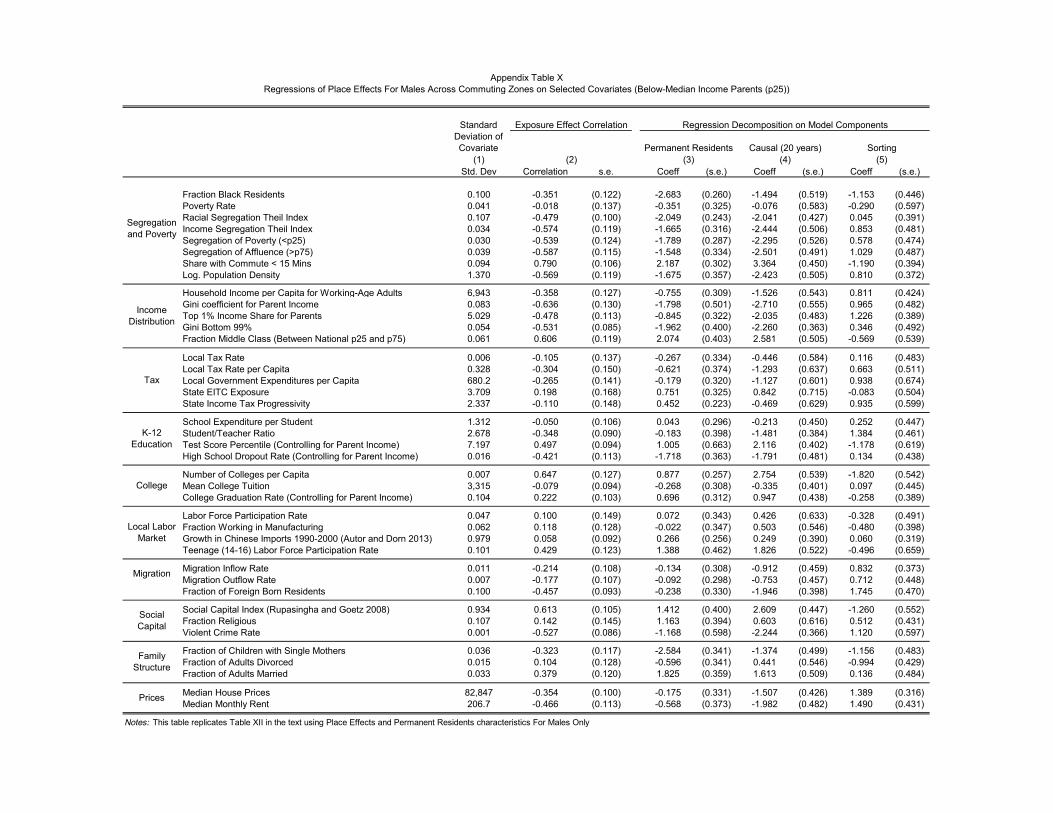
(1)Std. Dev Correlation s.e. Coeff (s.e.) Coeff (s.e.) Coeff (s.e.)

Fraction Black Residents 0.100 -0.351 (0.122) -2.683 (0.260) -1.494 (0.519) -1.153 (0.446)Poverty Rate 0.041 -0.018 (0.137) -0.351 (0.325) -0.076 (0.583) -0.290 (0.597)Racial Segregation Theil Index 0.107 -0.479 (0.100) -2.049 (0.243) -2.041 (0.427) 0.045 (0.391)Income Segregation Theil Index 0.034 -0.574 (0.119) -1.665 (0.316) -2.444 (0.506) 0.853 (0.481)Segregation of Poverty (<p25) 0.030 -0.539 (0.124) -1.789 (0.287) -2.295 (0.526) 0.578 (0.474)Segregation of Affluence (>p75) 0.039 -0.587 (0.115) -1.548 (0.334) -2.501 (0.491) 1.029 (0.487)Share with Commute < 15 Mins 0.094 0.790 (0.106) 2.187 (0.302) 3.364 (0.450) -1.190 (0.394)Log. Population Density 1.370 -0.569 (0.119) -1.675 (0.357) -2.423 (0.505) 0.810 (0.372)

Household Income per Capita for Working-Age Adults 6,943 -0.358 (0.127) -0.755 (0.309) -1.526 (0.543) 0.811 (0.424)Gini coefficient for Parent Income 0.083 -0.636 (0.130) -1.798 (0.501) -2.710 (0.555) 0.965 (0.482)Top 1% Income Share for Parents 5.029 -0.478 (0.113) -0.845 (0.322) -2.035 (0.483) 1.226 (0.389)Gini Bottom 99% 0.054 -0.531 (0.085) -1.962 (0.400) -2.260 (0.363) 0.346 (0.492)Fraction Middle Class (Between National p25 and p75) 0.061 0.606 (0.119) 2.074 (0.403) 2.581 (0.505) -0.569 (0.539)

Local Tax Rate 0.006 -0.105 (0.137) -0.267 (0.334) -0.446 (0.584) 0.116 (0.483)Local Tax Rate per Capita 0.328 -0.304 (0.150) -0.621 (0.374) -1.293 (0.637) 0.663 (0.511)Local Government Expenditures per Capita 680.2 -0.265 (0.141) -0.179 (0.320) -1.127 (0.601) 0.938 (0.674)State EITC Exposure 3.709 0.198 (0.168) 0.751 (0.325) 0.842 (0.715) -0.083 (0.504)State Income Tax Progressivity 2.337 -0.110 (0.148) 0.452 (0.223) -0.469 (0.629) 0.935 (0.599)

School Expenditure per Student 1.312 -0.050 (0.106) 0.043 (0.296) -0.213 (0.450) 0.252 (0.447)Student/Teacher Ratio 2.678 -0.348 (0.090) -0.183 (0.398) -1.481 (0.384) 1.384 (0.461)Test Score Percentile (Controlling for Parent Income) 7.197 0.497 (0.094) 1.005 (0.663) 2.116 (0.402) -1.178 (0.619)High School Dropout Rate (Controlling for Parent Income) 0.016 -0.421 (0.113) -1.718 (0.363) -1.791 (0.481) 0.134 (0.438)

Number of Colleges per Capita 0.007 0.647 (0.127) 0.877 (0.257) 2.754 (0.539) -1.820 (0.542)Mean College Tuition 3,315 -0.079 (0.094) -0.268 (0.308) -0.335 (0.401) 0.097 (0.445)College Graduation Rate (Controlling for Parent Income) 0.104 0.222 (0.103) 0.696 (0.312) 0.947 (0.438) -0.258 (0.389)

Labor Force Participation Rate 0.047 0.100 (0.149) 0.072 (0.343) 0.426 (0.633) -0.328 (0.491)Fraction Working in Manufacturing 0.062 0.118 (0.128) -0.022 (0.347) 0.503 (0.546) -0.480 (0.398)Growth in Chinese Imports 1990-2000 (Autor and Dorn 2013) 0.979 0.058 (0.092) 0.266 (0.256) 0.249 (0.390) 0.060 (0.319)Teenage (14-16) Labor Force Participation Rate 0.101 0.429 (0.123) 1.388 (0.462) 1.826 (0.522) -0.496 (0.659)

Migration Inflow Rate 0.011 -0.214 (0.108) -0.134 (0.308) -0.912 (0.459) 0.832 (0.373)Migration Outflow Rate 0.007 -0.177 (0.107) -0.092 (0.298) -0.753 (0.457) 0.712 (0.448)Fraction of Foreign Born Residents 0.100 -0.457 (0.093) -0.238 (0.330) -1.946 (0.398) 1.745 (0.470)

Social Capital Index (Rupasingha and Goetz 2008) 0.934 0.613 (0.105) 1.412 (0.400) 2.609 (0.447) -1.260 (0.552)Fraction Religious 0.107 0.142 (0.145) 1.163 (0.394) 0.603 (0.616) 0.512 (0.431)Violent Crime Rate 0.001 -0.527 (0.086) -1.168 (0.598) -2.244 (0.366) 1.120 (0.597)

Fraction of Children with Single Mothers 0.036 -0.323 (0.117) -2.584 (0.341) -1.374 (0.499) -1.156 (0.483)Fraction of Adults Divorced 0.015 0.104 (0.128) -0.596 (0.341) 0.441 (0.546) -0.994 (0.429)Fraction of Adults Married 0.033 0.379 (0.120) 1.825 (0.359) 1.613 (0.509) 0.136 (0.484)

Median House Prices 82,847 -0.354 (0.100) -0.175 (0.331) -1.507 (0.426) 1.389 (0.316)Median Monthly Rent 206.7 -0.466 (0.113) -0.568 (0.373) -1.982 (0.482) 1.490 (0.431)

Family Structure

Prices

Notes: This table replicates Table XII in the text using Place Effects and Permanent Residents characteristics For Males Only

Tax

K-12 Education

College

Local Labor Market

Migration

Social Capital

Income Distribution

Appendix Table XRegressions of Place Effects For Males Across Commuting Zones on Selected Covariates (Below-Median Income Parents (p25))

Standard Deviation of Covariate

Exposure Effect Correlation Regression Decomposition on Model Components

Permanent Residents Causal (20 years) Sorting(2) (3) (4) (5)

Segregation and Poverty

(1)Std. Dev Correlation s.e. Coeff (s.e.) Coeff (s.e.) Coeff (s.e.)

Fraction Black Residents 0.130 0.059 (0.206) -2.394 (0.202) 0.211 (0.734) -2.608 (0.742)Poverty Rate 0.055 0.016 (0.192) -1.983 (0.271) 0.056 (0.684) -2.048 (0.778)Racial Segregation Theil Index 0.118 -0.232 (0.083) -2.442 (0.163) -0.824 (0.294) -1.622 (0.310)Income Segregation Theil Index 0.039 -0.381 (0.129) -1.919 (0.129) -1.355 (0.460) -0.568 (0.469)Segregation of Poverty (<p25) 0.034 -0.401 (0.130) -2.028 (0.142) -1.427 (0.464) -0.607 (0.479)Segregation of Affluence (>p75) 0.045 -0.342 (0.127) -1.686 (0.138) -1.217 (0.451) -0.469 (0.449)Share with Commute < 15 Mins 0.102 -0.197 (0.264) 0.301 (0.201) -0.700 (0.940) 1.014 (0.941)Log. Population Density 1.718 -0.291 (0.128) -2.039 (0.296) -1.037 (0.456) -1.011 (0.504)

Household Income per Capita for Working-Age Adults 9,222 -0.127 (0.164) 0.729 (0.252) -0.453 (0.585) 1.181 (0.615)Gini coefficient for Parent Income 0.113 -0.226 (0.108) -2.102 (0.494) -0.804 (0.384) -1.294 (0.424)Top 1% Income Share for Parents 0.064 -0.076 (0.098) -1.093 (0.326) -0.270 (0.350) -0.819 (0.402)Gini Bottom 99% 0.112 -0.227 (0.108) -2.105 (0.493) -0.806 (0.384) -1.295 (0.424)Fraction Middle Class (Between National p25 and p75) 0.074 0.060 (0.154) 0.872 (0.275) 0.213 (0.548) 0.647 (0.563)

Local Tax Rate 0.009 -0.241 (0.294) -0.975 (0.687) -0.858 (1.046) -0.131 (0.841)Local Tax Rate per Capita 0.432 -0.204 (0.281) -0.530 (0.586) -0.728 (0.999) 0.190 (0.760)Local Government Expenditures per Capita 1.019 -0.212 (0.211) -1.106 (0.611) -0.755 (0.751) -0.368 (0.587)State EITC Exposure 3.750 -0.061 (0.121) -0.067 (0.059) -0.218 (0.432) 0.142 (0.440)State Income Tax Progressivity 2.365 -0.073 (0.167) -0.101 (0.138) -0.260 (0.594) 0.159 (0.649)

School Expenditure per Student 1.483 0.129 (0.195) -0.472 (0.424) 0.459 (0.695) -0.951 (0.777)Student/Teacher Ratio 2.816 -0.587 (0.481) -0.549 (0.226) -2.089 (1.712) 1.554 (1.760)Test Score Percentile (Controlling for Parent Income) 9.610 0.141 (0.128) 1.879 (0.417) 0.503 (0.456) 1.381 (0.537)High School Dropout Rate (Controlling for Parent Income) 0.024 -0.412 (0.289) -1.920 (0.248) -1.465 (1.028) -0.465 (1.052)

Number of Colleges per Capita 0.011 0.258 (0.157) -0.444 (0.199) 0.917 (0.557) -1.419 (0.531)Mean College Tuition 4,421 0.030 (0.122) -0.365 (0.267) 0.106 (0.434) -0.473 (0.488)College Graduation Rate (Controlling for Parent Income) 0.139 0.197 (0.171) -0.617 (0.206) 0.701 (0.608) -1.318 (0.597)

Labor Force Participation Rate 0.058 -0.327 (0.297) 0.882 (0.261) -1.164 (1.056) 2.076 (1.039)Fraction Working in Manufacturing 0.070 0.492 (0.280) 1.119 (0.163) 1.752 (0.998) -0.622 (1.010)Teenage (14-16) Labor Force Participation Rate 0.108 -0.345 (0.460) 1.020 (0.228) -1.229 (1.636) 2.250 (1.629)

Migration Inflow Rate 0.019 -0.144 (0.120) 1.104 (0.250) -0.512 (0.427) 1.627 (0.487)Migration Outflow Rate 0.014 -0.129 (0.137) 0.071 (0.244) -0.458 (0.488) 0.541 (0.515)Fraction of Foreign Born Residents 0.109 -0.018 (0.074) -0.776 (0.246) -0.064 (0.263) -0.709 (0.369)

Social Capital Index (Rupasingha and Goetz 2008) 1.096 0.045 (0.126) -0.146 (0.246) 0.159 (0.448) -0.321 (0.478)Fraction Religious 0.128 0.176 (0.159) -0.031 (0.185) 0.627 (0.565) -0.673 (0.563)Violent Crime Rate 0.002 -0.176 (0.085) -1.804 (0.170) -0.626 (0.302) -1.181 (0.339)

Fraction of Children with Single Mothers 0.069 -0.222 (0.130) -2.613 (0.316) -0.789 (0.464) -1.820 (0.541)Fraction of Adults Divorced 0.017 -0.227 (0.428) -1.777 (0.174) -0.806 (1.524) -0.977 (1.523)Fraction of Adults Married 0.062 0.073 (0.138) 2.551 (0.168) 0.260 (0.491) 2.290 (0.530)

Median House Price 124,001 -0.067 (0.087) 0.160 (0.378) -0.239 (0.310) 0.401 (0.612)Median Monthly Rent 217.8 -0.160 (0.213) 0.608 (0.246) -0.568 (0.759) 1.194 (0.724)

Family Structure

Prices

Notes: This table replicates Table XIV in the text using Place Effects and Permanent Residents characteristics For Males Only

Tax

K-12 Education

College

Local Labor Market

Migration

Social Capital

Income Distribution

Appendix Table XIRegressions of Place Effects for Males Across Counties within Commuting Zones on Selected Covariates (Below-Median Income Parents (p25))

Standard Deviation of Covariate

Exposure Effect Correlation Regression Decomposition on Model Components

Permanent Residents Causal (20 years) Sorting(2) (3) (4) 5)

Segregation and Poverty

(1)Std. Dev Correlation s.e. Coeff (s.e.) Coeff (s.e.) Coeff (s.e.)

Fraction Black Residents 0.100 -0.430 (0.125) -2.163 (0.242) -1.371 (0.398) -0.763 (0.428)Poverty Rate 0.041 -0.137 (0.113) -0.756 (0.289) -0.436 (0.361) -0.324 (0.437)Racial Segregation Theil Index 0.107 -0.348 (0.147) -1.344 (0.262) -1.110 (0.468) -0.185 (0.519)Income Segregation Theil Index 0.034 -0.312 (0.150) -0.620 (0.304) -0.995 (0.480) 0.448 (0.528)Segregation of Poverty (<p25) 0.030 -0.321 (0.157) -0.787 (0.281) -1.023 (0.500) 0.306 (0.525)Segregation of Affluence (>p75) 0.039 -0.297 (0.142) -0.506 (0.312) -0.949 (0.455) 0.515 (0.515)Share with Commute < 15 Mins 0.094 0.608 (0.175) 1.081 (0.350) 1.940 (0.558) -0.914 (0.577)Log. Population Density 1.368 -0.503 (0.129) -0.619 (0.340) -1.603 (0.413) 1.062 (0.484)

Household Income per Capita for Working-Age Adults 6,943 -0.135 (0.133) 0.310 (0.266) -0.429 (0.424) 0.774 (0.380)Gini coefficient for Parent Income 0.083 -0.540 (0.132) -0.984 (0.502) -1.722 (0.420) 0.788 (0.545)Top 1% Income Share for Parents 5.028 -0.302 (0.114) 0.139 (0.266) -0.963 (0.364) 1.148 (0.347)Gini Bottom 99% 0.054 -0.545 (0.150) -1.634 (0.388) -1.739 (0.477) 0.148 (0.559)Fraction Middle Class (Between National p25 and p75) 0.061 0.485 (0.165) 1.171 (0.416) 1.548 (0.527) -0.448 (0.580)

Local Tax Rate 0.006 -0.107 (0.137) 0.236 (0.286) -0.342 (0.437) 0.544 (0.436)Local Tax Rate per Capita 0.328 -0.174 (0.172) 0.412 (0.321) -0.557 (0.549) 0.966 (0.519)Local Government Expenditures per Capita 676.9 -0.044 (0.134) 0.635 (0.251) -0.140 (0.427) 0.778 (0.441)State EITC Exposure 3.709 -0.039 (0.178) 0.845 (0.279) -0.124 (0.566) 0.972 (0.484)State Income Tax Progressivity 2.337 0.067 (0.101) 0.729 (0.210) 0.214 (0.323) 0.527 (0.343)

School Expenditure per Student 1.312 -0.060 (0.176) 0.449 (0.293) -0.191 (0.562) 0.639 (0.503)Student/Teacher Ratio 2.678 -0.004 (0.128) 0.276 (0.373) -0.013 (0.410) 0.358 (0.510)Test Score Percentile (Controlling for Parent Income) 7.196 0.167 (0.123) 0.568 (0.666) 0.534 (0.391) -0.032 (0.591)High School Dropout Rate (Controlling for Parent Income) 0.016 -0.372 (0.156) -1.543 (0.330) -1.187 (0.499) -0.300 (0.452)

Number of Colleges per Capita 0.007 0.399 (0.144) 0.241 (0.267) 1.272 (0.460) -1.066 (0.413)Mean College Tuition 3,315 -0.307 (0.111) 0.031 (0.267) -0.978 (0.356) 1.029 (0.387)College Graduation Rate (Controlling for Parent Income) 0.104 -0.058 (0.101) 0.354 (0.235) -0.184 (0.322) 0.523 (0.317)

Labor Force Participation Rate 0.047 0.095 (0.114) 0.488 (0.259) 0.304 (0.362) 0.198 (0.366)Fraction Working in Manufacturing 0.062 -0.018 (0.159) -0.424 (0.274) -0.059 (0.508) -0.343 (0.560)Growth in Chinese Imports 1990-2000 (Autor and Dorn 2013) 0.979 -0.118 (0.129) 0.106 (0.218) -0.375 (0.411) 0.515 (0.359)Teenage (14-16) Labor Force Participation Rate 0.101 0.296 (0.170) 1.196 (0.483) 0.945 (0.542) 0.201 (0.623)

Migration Inflow Rate 0.011 -0.004 (0.140) 0.046 (0.258) -0.014 (0.447) 0.101 (0.390)Migration Outflow Rate 0.007 0.052 (0.142) 0.514 (0.281) 0.166 (0.452) 0.392 (0.360)Fraction of Foreign Born Residents 0.100 -0.198 (0.123) 0.616 (0.254) -0.633 (0.393) 1.281 (0.382)

Social Capital Index (Rupasingha and Goetz 2008) 0.934 0.365 (0.159) 1.013 (0.398) 1.164 (0.508) -0.211 (0.531)Fraction Religious 0.107 0.056 (0.183) 0.949 (0.351) 0.179 (0.583) 0.737 (0.441)Violent Crime Rate 0.001 -0.414 (0.182) -0.764 (0.603) -1.322 (0.580) 0.596 (0.538)

Fraction of Children with Single Mothers 0.036 -0.501 (0.129) -2.329 (0.371) -1.598 (0.412) -0.682 (0.552)Fraction of Adults Divorced 0.015 0.089 (0.160) -0.803 (0.259) 0.282 (0.509) -1.052 (0.427)Fraction of Adults Married 0.033 0.430 (0.152) 1.080 (0.378) 1.373 (0.484) -0.364 (0.555)

Median House Prices 82,845 -0.139 (0.171) 0.739 (0.226) -0.445 (0.546) 1.234 (0.452)Median Monthly Rent 206.7 -0.200 (0.165) 0.550 (0.304) -0.639 (0.525) 1.258 (0.406)

Family Structure

Prices

Notes: This table replicates Table XII in the text using Place Effects and Permanent Residents characteristics for Females Only

Tax

K-12 Education

College

Local Labor Market

Migration

Social Capital

Income Distribution

Appendix Table XIIRegressions of Place Effects for Females Across Commuting Zones on Selected Covariates (Below-Median Income Parents (p25))

Standard Deviation of Covariate

Exposure Effect Correlation Regression Decomposition on Model Components

Permanent Residents Causal (20 years) Sorting(2) (3) (4) (5)

Segregation and Poverty

(1)Std. Dev Correlation s.e. Coeff (s.e.) Coeff (s.e.) Coeff (s.e.)

Fraction Black Residents 0.130 -0.371 (0.255) -2.131 (0.159) -0.486 (0.334) -1.646 (0.347)Poverty Rate 0.055 0.139 (0.478) -1.940 (0.199) 0.183 (0.626) -2.129 (0.600)Racial Segregation Theil Index 0.118 -0.452 (0.281) -2.049 (0.140) -0.593 (0.368) -1.459 (0.363)Income Segregation Theil Index 0.039 -0.488 (0.237) -1.451 (0.113) -0.640 (0.311) -0.806 (0.298)Segregation of Poverty (<p25) 0.034 -0.540 (0.244) -1.596 (0.129) -0.708 (0.320) -0.885 (0.311)Segregation of Affluence (>p75) 0.045 -0.420 (0.241) -1.224 (0.122) -0.551 (0.316) -0.668 (0.302)Share with Commute < 15 Mins 0.102 0.335 (0.530) 0.174 (0.199) 0.439 (0.694) -0.253 (0.756)Log. Population Density 1.715 -0.453 (0.306) -1.520 (0.269) -0.593 (0.401) -0.927 (0.433)

Household Income per Capita for Working-Age Adults 9,222 -0.222 (0.348) 0.921 (0.263) -0.291 (0.456) 1.210 (0.394)Gini coefficient for Parent Income 0.113 -0.775 (0.325) -1.783 (0.358) -1.016 (0.426) -0.766 (0.346)Top 1% Income Share for Parents 0.064 -0.693 (0.455) -0.812 (0.214) -0.909 (0.596) 0.100 (0.576)Gini Bottom 99% 0.112 -0.775 (0.324) -1.786 (0.357) -1.015 (0.424) -0.770 (0.345)Fraction Middle Class (Between National p25 and p75) 0.075 -0.086 (0.348) 0.516 (0.263) -0.112 (0.456) 0.614 (0.438)

Local Tax Rate 0.009 0.234 (0.795) -0.808 (0.619) 0.306 (1.042) -1.132 (1.425)Local Tax Rate per Capita 0.432 0.005 (0.499) -0.316 (0.463) 0.007 (0.654) -0.331 (0.989)Local Government Expenditures per Capita 1.016 -0.502 (0.223) -0.954 (0.532) -0.657 (0.292) -0.312 (0.628)State EITC Exposure 3.752 0.449 (0.381) -0.105 (0.065) 0.588 (0.500) -0.703 (0.460)State Income Tax Progressivity 2.365 -0.039 (0.599) -0.164 (0.125) -0.051 (0.785) -0.114 (0.834)

School Expenditure per Student 1.483 1.135 (1.332) -0.240 (0.405) 1.488 (1.745) -1.749 (1.872)Student/Teacher Ratio 2.816 -0.317 (0.371) -0.575 (0.231) -0.416 (0.486) -0.143 (0.583)Test Score Percentile (Controlling for Parent Income) 9.612 0.346 (0.490) 1.654 (0.335) 0.454 (0.642) 1.202 (0.688)High School Dropout Rate (Controlling for Parent Income) 0.024 -0.449 (0.348) -1.682 (0.205) -0.589 (0.456) -1.105 (0.458)

Number of Colleges per Capita 0.011 0.201 (0.863) -0.491 (0.197) 0.264 (1.130) -0.810 (1.128)Mean College Tuition 4,421 -0.079 (0.296) -0.305 (0.249) -0.103 (0.387) -0.206 (0.520)College Graduation Rate (Controlling for Parent Income) 0.139 -0.374 (0.359) -0.480 (0.207) -0.491 (0.471) 0.007 (0.511)

Labor Force Participation Rate 0.058 -0.116 (0.502) 1.019 (0.225) -0.152 (0.658) 1.189 (0.656)Fraction Working in Manufacturing 0.070 0.272 (0.370) 0.818 (0.140) 0.356 (0.484) 0.473 (0.476)Teenage (14-16) Labor Force Participation Rate 0.108 -0.065 (0.497) 1.075 (0.201) -0.085 (0.651) 1.160 (0.629)

Migration Inflow Rate 0.019 -0.227 (0.277) 0.938 (0.217) -0.297 (0.363) 1.247 (0.371)Migration Outflow Rate 0.014 -0.070 (0.349) 0.203 (0.247) -0.092 (0.457) 0.309 (0.453)Fraction of Foreign Born Residents 0.109 -0.081 (0.371) -0.500 (0.202) -0.107 (0.486) -0.390 (0.456)

Social Capital Index (Rupasingha and Goetz 2008) 1.096 0.370 (0.604) 0.072 (0.219) 0.485 (0.791) -0.426 (0.815)Fraction Religious 0.128 -0.230 (0.380) 0.050 (0.179) -0.302 (0.497) 0.334 (0.518)Violent Crime Rate 0.002 -0.681 (0.320) -1.713 (0.132) -0.892 (0.419) -0.822 (0.387)

Fraction of Children with Single Mothers 0.069 -0.429 (0.268) -2.392 (0.212) -0.562 (0.352) -1.826 (0.265)Fraction of Adults Divorced 0.017 -0.763 (0.404) -1.617 (0.169) -0.999 (0.529) -0.629 (0.542)Fraction of Adults Married 0.062 0.304 (0.299) 2.245 (0.113) 0.398 (0.392) 1.845 (0.387)

Median House Price 124,012 -0.182 (0.139) 0.173 (0.461) -0.239 (0.182) 0.413 (0.437)Median Monthly Rent 217.7 0.058 (0.340) 0.940 (0.219) 0.076 (0.445) 0.877 (0.466)

Family Structure

Prices

Notes: This table replicates Table XIV in the text using Place Effects and Permanent Residents characteristics For Females Only

Appendix Table XIIIRegressions of Place Effects for Females Across Counties within Commuting Zones on Selected Covariates (Below-Median Income Parents (p25))

Exposure Effect Correlation Regression Decomposition on Model Components

Permanent Residents Causal (20 years) Sorting

Tax

K-12 Education

College

Local Labor Market

Migration

Social Capital

5)

Standard Deviation of Covariate

Segregation and Poverty

Income Distribution

(2) (3) (4)

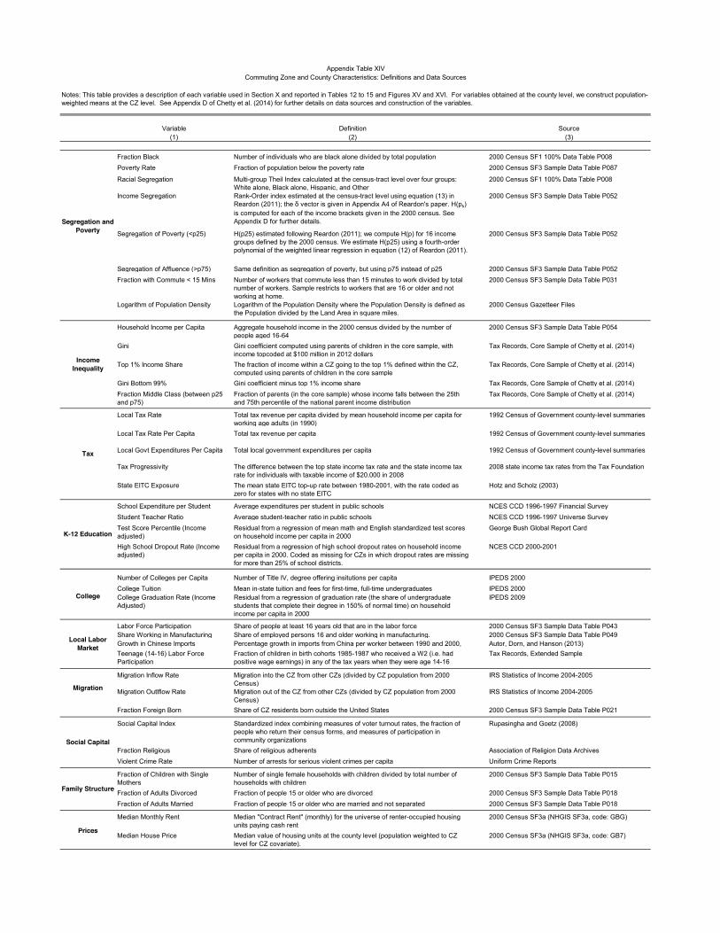
Variable Definition Source(1) (2) (3)

Fraction Black Number of individuals who are black alone divided by total population 2000 Census SF1 100% Data Table P008Poverty Rate Fraction of population below the poverty rate 2000 Census SF3 Sample Data Table P087

Racial Segregation Multi-group Theil Index calculated at the census-tract level over four groups: White alone, Black alone, Hispanic, and Other

2000 Census SF1 100% Data Table P008

Income Segregation Rank-Order index estimated at the census-tract level using equation (13) in Reardon (2011);; the δ vector is given in Appendix A4 of Reardon's paper. H(pk) is computed for each of the income brackets given in the 2000 census. See Appendix D for further details.

2000 Census SF3 Sample Data Table P052

Segregation of Poverty (<p25) H(p25) estimated following Reardon (2011); we compute H(p) for 16 income groups defined by the 2000 census. We estimate H(p25) using a fourth-order polynomial of the weighted linear regression in equation (12) of Reardon (2011).

2000 Census SF3 Sample Data Table P052

Segregation of Affluence (>p75) Same definition as segregation of poverty, but using p75 instead of p25 2000 Census SF3 Sample Data Table P052Fraction with Commute < 15 Mins Number of workers that commute less than 15 minutes to work divided by total

number of workers. Sample restricts to workers that are 16 or older and not working at home.

2000 Census SF3 Sample Data Table P031

Logarithm of Population Density Logarithm of the Population Density where the Population Density is defined as the Population divided by the Land Area in square miles.

2000 Census Gazetteer Files

Household Income per Capita Aggregate household income in the 2000 census divided by the number of people aged 16-64

2000 Census SF3 Sample Data Table P054

Gini Gini coefficient computed using parents of children in the core sample, with income topcoded at $100 million in 2012 dollars

Tax Records, Core Sample of Chetty et al. (2014)

Top 1% Income Share The fraction of income within a CZ going to the top 1% defined within the CZ, computed using parents of children in the core sample

Tax Records, Core Sample of Chetty et al. (2014)

Gini Bottom 99% Gini coefficient minus top 1% income share Tax Records, Core Sample of Chetty et al. (2014)Fraction Middle Class (between p25 and p75)

Fraction of parents (in the core sample) whose income falls between the 25th and 75th percentile of the national parent income distribution

Tax Records, Core Sample of Chetty et al. (2014)

Local Tax Rate Total tax revenue per capita divided by mean household income per capita for working age adults (in 1990)

1992 Census of Government county-level summaries

Local Tax Rate Per Capita Total tax revenue per capita 1992 Census of Government county-level summaries

Local Govt Expenditures Per Capita Total local government expenditures per capita 1992 Census of Government county-level summaries

Tax Progressivity The difference between the top state income tax rate and the state income tax rate for individuals with taxable income of $20,000 in 2008

2008 state income tax rates from the Tax Foundation

State EITC Exposure The mean state EITC top-up rate between 1980-2001, with the rate coded as zero for states with no state EITC

Hotz and Scholz (2003)

School Expenditure per Student Average expenditures per student in public schools NCES CCD 1996-1997 Financial SurveyStudent Teacher Ratio Average student-teacher ratio in public schools NCES CCD 1996-1997 Universe SurveyTest Score Percentile (Income adjusted)

Residual from a regression of mean math and English standardized test scores on household income per capita in 2000

George Bush Global Report Card

High School Dropout Rate (Income adjusted)

Residual from a regression of high school dropout rates on household income per capita in 2000. Coded as missing for CZs in which dropout rates are missing for more than 25% of school districts.

NCES CCD 2000-2001

Number of Colleges per Capita Number of Title IV, degree offering insitutions per capita IPEDS 2000College Tuition Mean in-state tuition and fees for first-time, full-time undergraduates IPEDS 2000College Graduation Rate (Income Adjusted)

Residual from a regression of graduation rate (the share of undergraduate students that complete their degree in 150% of normal time) on household income per capita in 2000

IPEDS 2009

Labor Force Participation Share of people at least 16 years old that are in the labor force 2000 Census SF3 Sample Data Table P043Share Working in Manufacturing Share of employed persons 16 and older working in manufacturing. 2000 Census SF3 Sample Data Table P049Growth in Chinese Imports Percentage growth in imports from China per worker between 1990 and 2000,

scaled as an annualized rate times 10Autor, Dorn, and Hanson (2013)

Teenage (14-16) Labor Force Participation

Fraction of children in birth cohorts 1985-1987 who received a W2 (i.e. had positive wage earnings) in any of the tax years when they were age 14-16

Tax Records, Extended Sample

Migration Inflow Rate Migration into the CZ from other CZs (divided by CZ population from 2000 Census)

IRS Statistics of Income 2004-2005

Migration Outlflow Rate Migration out of the CZ from other CZs (divided by CZ population from 2000 Census)

IRS Statistics of Income 2004-2005

Fraction Foreign Born Share of CZ residents born outside the United States 2000 Census SF3 Sample Data Table P021

Social Capital Index Standardized index combining measures of voter turnout rates, the fraction of people who return their census forms, and measures of participation in community organizations

Rupasingha and Goetz (2008)

Fraction Religious Share of religious adherents Association of Religion Data ArchivesViolent Crime Rate Number of arrests for serious violent crimes per capita Uniform Crime Reports

Fraction of Children with Single Mothers

Number of single female households with children divided by total number of households with children

2000 Census SF3 Sample Data Table P015

Fraction of Adults Divorced Fraction of people 15 or older who are divorced 2000 Census SF3 Sample Data Table P018Fraction of Adults Married Fraction of people 15 or older who are married and not separated 2000 Census SF3 Sample Data Table P018

Median Monthly Rent Median "Contract Rent" (monthly) for the universe of renter-occupied housing units paying cash rent

2000 Census SF3a (NHGIS SF3a, code: GBG)

Median House Price Median value of housing units at the county level (population weighted to CZ level for CZ covariate).

2000 Census SF3a (NHGIS SF3a, code: GB7)

Appendix Table XIVCommuting Zone and County Characteristics: Definitions and Data Sources

Prices

Notes: This table provides a description of each variable used in Section X and reported in Tables 12 to 15 and Figures XV and XVI. For variables obtained at the county level, we construct population-weighted means at the CZ level. See Appendix D of Chetty et al. (2014) for further details on data sources and construction of the variables.

Segregation and Poverty

Income Inequality

Tax

K-12 Education

College

Local Labor Market

Migration

Social Capital

Family Structure