child benefit and fiscal burden with endogenous fertility · moreover, the baby boomer generation...
TRANSCRIPT

Munich Personal RePEc Archive
Child Benefit and Fiscal Burden with
Endogenous Fertility
Oguro, Kazumasa and Takahata, Junichiro
Graduate School of Economics, Hitotsuashi University
April 2009
Online at https://mpra.ub.uni-muenchen.de/15378/
MPRA Paper No. 15378, posted 25 May 2009 09:40 UTC

1
Child Benefit and Fiscal Burden with Endogenous Fertility1
Kazumasa Oguro Research fellow, Institute for International Policy Studies
Consulting fellow, Research Institute of Economy, Trade and Industry,
Ministry of Economy, Trade and Industry, Government of Japan [email protected]
and
Junichiro Takahata Graduate School of Economics, Hitotsubashi University
Researcher, Policy Research Institute, Ministry of Finance, Government of Japan
This version: April 2009
Abstract This paper studies a possibility of efficiency improvement by child benefit programs in an overlapping
generations economy with endogenous fertility and government debt. We derive conditions for improving an
efficiency by child benefit using Representative-Consumer efficiency (RC-efficiency), an efficiency criterion
for an endogenous fertility setting developed by Michel and Wigniolle (2007).
It is shown that the result crucially depends on the relative amount of accumulated government debt in
the economy. It is likely to hold in an economy of developed countries with a low fertility rate. We provide an
implication of the results in the real economy.
Keywords: Endogenous fertility, Pareto-efficiency, child benefit, fiscal burden
JEL Classification Numbers D9, J13, D61
1. Introduction
The purpose of this paper is to analyze the relationship between child benefit and fiscal
burden in the setting of an overlapping generation model with endogenous fertility.
Lump-sum tax and public debt can be resources of child benefit. Although the tax burden of
each generation is concentrated on its respective working period, this period also
corresponds to the child-rearing period in some cases. Therefore, implementing child
1 This paper was presented at the First Workshop on Demography and Public Finance at Hitotsubashi University in March 7, 2009. We are grateful for helpful comments and discussions from Takashi OSHIO (Professor, Graduate School of Economics, Hitotsubashi University (Kobe University until March 2009)), Motohiro SATO (Associate Professor, Graduate School of Economics, Hitotsubashi University), Ryo ISHIDA (University of Michigan, US), and the workshop participants. Takahata was supported by a grant from Global COE program “Research Unit for Statistical and Empirical Analysis in Social Sciences.” Finally, the opinions expressed in this paper are those of the authors and do not represent the views of the organizations to which we belong. Any remaining errors are the responsibility of the authors.

2
benefit programs financed by lump-sum tax in an exogenous fertility setting is a zero-sum
game in that it transfers the fiscal burden to the same generation. On the other hand,
financing child benefit programs by issuing debt is a zero-sum game in that it transfers the
fiscal burden from the current generation to the future generation. In this paper, we focus
mainly on child benefit financed by public debt in an endogenous fertility setting. Also, if
certain conditions are satisfied, we clarify that the benefit has the potential to improve each
generation's utility through the mitigation of per-capita fiscal burden.
In industrialized countries, the fiscal burden has been increasing. In Japan, especially,
the debt-GDP ratio is the highest among industrialized countries, even beyond that of Italy.
As is well known, the sustainability of the Japanese fiscal and social security system is
declining because of its low fertility rate, aging, and decreasing population. This situation is
due to the fact that Japan now holds public debt explicitly and implicitly: the explicit debt
is about 180% to GDP with regard to government bonds and the implicit debt is about
230% with regard to the social security system, public pension, medical insurance, and
elderly assistance. Therefore, Japan holds a total of approximately 410% public debt to
GDP.
Table1. Public Debt-GDP ratio and Total Fertility Rate (TFR) of Industrialized Countries Country Japan Italy France Germany UK US
Public
Debt
1.71 1.17 0.71 0.64 0.50 0.66
TFR 1.33 1.32 1.87 1.28 1.66 2.04
Source: United Nations (2006) “Population, Resources, Environment and Development.”
Moreover, the baby boomer generation comprising the largest population is now
moving over to the benefit side of the social security system. Thus, attempts to reduce the
benefit will face political limitations. This means that the 410% public debt must be paid
mainly by the current working generation and future generations.
In addition, the fertility rate in Japan has been decreasing since the baby boom in the
1950s. To maintain the population level, it is considered necessary for a woman to have
2.08 children. The total fertility rate in Japan was above 2.08 before the 1970s, but since
then, it has fallen below that number. The relationship between (explicit) debt-GDP ratio
and fertility rate in developed countries is shown in Table 1.
These demographic factors raise the following question: what is the most economically
efficient way for the burden to be shared by each generation? The answer will essentially
differ depending on whether the model is exogenous fertility or endogenous fertility.
For this reason recent studies have clarified that the Pareto-efficiency condition of the
exogenous fertility model differs from that of endogenous. First, in the case of an
exogenous fertility model, we make use of the overlapping generations (OLG) model which
was introduced by Diamond (1965). Three types of steady states exist in the model:
under-accumulation, golden rule, and over-accumulation. The first two steady states are
Pareto-efficient, but the third is not. In addition, an empirical study by Abel, Mankiw,
Summers, and Zeckhauser (1989) reports that in industrialized countries dynamic
efficiency is satisfied. In a steady state, dynamic efficiency corresponds to

3
under-accumulation (or golden rule). Therefore, the possibility that industrialized countries
are in the state of under-accumulation seems high. In an exogenous fertility setting, an
allocation is said to be Pareto-efficient if it is impossible to make some individuals better
off without making other individuals worse off. For this reason, in an exogenous case, we
cannot improve any generation's utility while at the same time sacrificing another
generation's utility.
However, recent studies clarify the properties of the competitive equilibrium with an
endogenous fertility setting. Raut and Srinivasan (1994) and Charkrabarti (1999) analyze
the properties of the inter-temporal equilibrium with endogenous fertility. Conde-Ruiz et al.
(2002) and Golosov et al. (2004) present the definition of Pareto-efficiency criteria in an
endogenous fertility framework.
As a development of these studies, surprisingly, Michel and Wigniolle (2007)2 point
out the possibility that under-accumulation may not be efficient in an endogenous fertility
setting. This implies that there is a possibility of improving one generation's welfare
without making another generation's welfare worse off by some policies, even when it is in
an under-accumulation state near the steady state. Moreover, the remarkable point of
Michel and Wigniolle (2007) is to clarify that the Representative-Consumer efficient
(RC-efficient) condition, which is a concept developed in their study, deeply connects with
the sign-of-inequality relationship between the child-rearing cost and wage rate. That is, if
by some policies we can give some effects to this relationship, we would have a possibility
to improve RC-efficiency.
Michel and Wigniolle (2007) provide proof that, by utilizing an OLG model with
endogenous population growth, the possibility to improve RC-efficiency also exists in the
case of under-accumulation. But they did not analyze an economy model with public debt.
Therefore, we have great interest in the possibility of improving RC-efficiency in an
economy with huge public debt, low fertility rate, and endogenous population growth.
Therefore, we should focus on the child benefit programs financed by debt. The policy
has the possibility to affect the conditions of RC-efficiency through the following path.
First, there is a path of reducing the per-capita fiscal burden through fertility rate increase,
which is found in even a simple model without capital accumulation. Second, as is shown
in a model with capital accumulation, child benefit may affect an individual’s expenditure
through the current fertility level and interest rate which causes the consumption amount in
the second period. The first condition has particular effect when an economy holds huge
public debt like that of Japan.
Intuitively, there is a possibility to attain RC-improvement by a child benefit program
financed by newly issued debt when the accumulated amount of debt is huge. This is
because of the following logic. Suppose we have a child benefit program financed by newly
issued debt and it raises the fertility rate to a certain level. An influence of newly issued
2Although there have been several approaches that endogenize fertility decisions, Michel and Wigniolle (2007) depend on the benchmark framework, which assumes that children are consumption goods that appear in the utility function of the parents. The basic articles are Becker (1960), Willis (1973), and Eckstein and Wolpin (1985). Other approaches depend on the literature based on the additional assumption of descendant altruism, as in Becker and Barro (1988) or the assumption of ascendant altruism and strategic behavior of parents, as in Nishimura and Zhang (1992).

4
debt to the accumulated debt is different depending on the size of accumulated debt. If the
effect of the rise in fertility is the same regardless of the amount of accumulated debt, then
such a policy may lessen per-capita debt without harming any generation. In this scenario,
even the initial generation is not made worse off since they do not need to endure the
burden. The problem of worsening the situation of the initial generation might occur if a
child benefit program were financed by a lump-sum tax. We will show situation using a
simple model first intuitively, and derive conditions in a general setting after that.
This paper is organized as follows. In Section 2 we introduce a simple model for
grasping an intuitive understanding. In Section 3, we will set the model for our main
analysis. In Section 4, we derive the conditions of RC-improvement using the model. In
Section 5, we analyze the superiority of public debt and tax with child benefit financing, as
continuing discussions of Sections 3 and 4.. Section 6 presents some concluding remarks.
2. Simple analysis In this section, we analyze a simple model to show the characteristics of child benefit
financed by public debt as preparation for analyzing the rigorous model in the next section.
As an example, we first make an intuitive analysis of the relationship between child benefit
and fiscal burden in a case with intergeneration-selfishness in a simple economy with only
two generations: parent generation and child generation. Next, by using an OLG model
with only two generations, we show the possibility that the child benefit improves
RC-efficiency.
First,, for simplicity, we consider the economy only with two generations, the first and
the second generation. Individuals live two periods, young and old, and they have children
when they are young. We assume that the second (young) generation does not have
children, and that the government expenditure is set to zero in the baseline case. The debt
amount at the beginning is set to D , and the government subsidizes per child for
child-rearing activity, financed by issuing bonds. In this simple model, we let N denote
the population of the first generation, nN that of the second generation, r interest rate,
z child-rearing cost, j
X and j
Y the consumption when young and old, W the lifetime
income, and the fiscal burden in lump-sum tax j
T ( 2,1j ). Using the above, we get the
following budget constraints for a representative household:
11
1
11
)( TWr
YXnz
(1)
22
2
21
TWr
YX
(2)
The intertemporal government budget constraint is the following:
nNr
TNTnND
1
2
1 (3)
Solving per capita fiscal burden of the second generation from equation (1) to (3), we
get the following relationship:
nN
NTnNDrT 1
2)1(
(4)
If 0/2
T is satisfied, enlarging child benefit programs financed by bond will

5
decrease the fiscal burden of the second generation. It is possible to rewrite the condition as
in the following:
nn
d
n
nTNDdwhere
n and/,
1 (5)
The left-hand side represents the fiscal burden of the second generation. On the other
hand, the denominator of the right-hand side represents the elasticity of fertility to child
benefit programs. As long as the ratio of child-rearing subsidy to elasticity is less than the
per capita fiscal burden of the second generation, the child benefit programs decrease the
per capita fiscal burden of the second generation. Specifically, the after-tax lifetime income
of the second generation increases, which implies that the lifetime utility rises. The lifetime
utility of the first generation also rises by the child benefit programs financed by bonds. In
other words, in the case equation (5) holds, child-rearing policy financed by bonds may
attain RC-improvement.
3. Model In this section, we construct the model for considering the condition for having the
child benefit financed by bonds to effect RC-improvement. The detailed settings are shown
in the following.
3.1. Household
Generation t lives two periods, period t when they are young and period 1t when
old, earn lifetime income W , enjoy consumption t
X when young and 1tY when old, and
raise children t
n at cost z , subsidized with t
. Generation t has to take over per capita
debt t
d from generation 1t by paying lump-sum tax t
T when young, and give their per
capita debt 1td to the following generation 1t when old.
Assumption 1 U is a function from 3
R to }{R , and U maps 3
R to R , with
./),,(everyfor ),,(lim),,( 33
),,(),,(
RRYXnYXnUYXnUYXnYXn
U is twice continuously differentiable on 3
R , strictly concave, increasing in each
argument, homogeneous of degree one, and satisfies the Inada conditions:
.limlimlim000
YY
XX
nn
UUU
In this case, the lifetime utility and the budget constraint of generation t is described
in the following:
),,(1
ttttYXnUU (6)
ttttttTWSXnz )( (7)
tttSRY
11 (8)
The first-order conditions for maximizing the lifetime utility are as follows:
t
n
YtXz
UURU
1
(9)

6
From the above equations, we can derive the following relationships:
),,(1 ttttt
RTWXX (10)
),,(11 ttttt
RTWYY (11)
),,(1 ttttt
RTWnn (12)
),,(1 ttttt
RTWSS (13)
Functions X , Y , n , s are defined on 3
R and are continuously differentiable.
3.2. Firm
We assume that, in period t , there exists a representative firm producing goods with
capital t
K and labor t
L under perfect competition using the following function which is
homogeneous of degree one and we can define f as )1,()( kFkf .
),(ttt
LKFQ (14)
Assumption 2 RR:f , and for all 0k , 0)( kf and 0)( kf .
Then we get the following condition from profit maximization:
t
t
t
t
t
t
t
t
tL
KW
L
Kf
L
K
L
KfW (15)
t
t
t
t
tL
KR
L
KfR (16)
3.3. Government
Suppose that the population of generation t is expressed as 11
tttNnN , and that the
government subsidizes child-rearing under the following budget constraint: the
reimbursement of per capita debt of generation 1t and child-rearing subsidy t
are
financed by lump-sum tax t
T and newly issued bond t
d :
)(11111
ttttttttttNnNdRNdNT
⇔ ttt
t
tt
tdR
n
dRT
1
1
1 (17)
3.4. Market equilibrium
Suppose that the labor market is balanced as tt
NL , and that the capital and the saving
in the capital market are balanced. Then, with ttt
NKk / , we have the following:
)(and)(tttt
kRRkWW (18)
)(1 tttt
dSNK (19)
The equation (19) is verified to be equivalent to the following commodity market
clearing condition by simple operation:

7
ttttt
t
t
ttttnRzn
n
YXknkf
1
1
1)( (20)
Definition 1 Starting from initial conditions 1N ,
0N ,
0K , and ))/((
10100 NKdRY ,
given debt management policies and child-rearing subsidies }),{(0
ttt
d , an inter-temporal
equilibrium is a sequence }),,,,{(0
tttttt
nYXNK , which satisfies (7)-(9) and (17)-(19).
4. The inter-temporal equilibrium In this section, based on the model constructed above, we will examine the condition
for the child benefit financed by issuing bonds to effect RC-improvement. Then an example
with a simple function is considered.
First, we will derive the condition of child benefit programs to improve lifetime utility
of all generations without sacrificing welfare of any generation. It is difficult to derive such
a condition rigorously in an analytical sense. In this paper, for simplicity, we assume that
)(t
UU is homogeneous of degree one. In addition, we define the variables as the
following:
tt
t
tTW
nn
~
tt
t
tTW
XX
~
tt
t
tTW
YY
1
1
~ (21)
tt
t
tTW
SS
~
.~
tt
t
tTW
dd
.~
tt
t
tTW
UU
The government budget constraint can be rewritten as
t
ttttn
dR
t
d
dWRT t
tt
~1
~1
~
~
1
1
And the budget constraints (7) and (8) can be transformed as the following:
1
~~~)(
1
t
t
tttR
YXnz (22)
From equation (9) and (22), we can solve the variables of equation (21) as a function of
),(1
ttRz . Substituting these variables into (19), we obtain the following:
ttttttttdRzSkRzn~
),(~
),(~111 (23)
)(11 ttt
kk
Proposition 1 Given 000
/ NKk and })~
{(0
tt
d , an inter-temporal equilibrium is

8
characterized by the sequence }){(0
tt
such that 0t ,
ttttttttdkRzSkkRzn~
)](,[~
)](,[~111
(24)
The proof is straightforward. A sequence 0
)( ttk is characterized by a sequence
0)( tt
in this setting, while an inter-temporal equilibrium is characterized by a sequence 0
)( ttk in
Michel and Wigniolle (2007). Hence, an inter-temporal equilibrium is characterized by a
sequence 0
)( tt .
We define the function as:
dkfzskkfznkz~
)](,[~)](,[~),(
is defined on 2
R and continuously differentiable. The equation (24) can be written
as: 0))(,(
1 ttt
kz
In this setting, the equation is no more dynamic since the function is only of 1tk but
not of t
k . Since 1tk is a function of
t , once we have a sequence of
0)( tt
, a unique
inter-temporal equilibrium 0
)( tt may exist. We would like to show this in the following.
Before that, we need to make some assumptions on saving and fertility to the change of
interest rate and child benefit.
In the following we will deal with several cases in terms of preferences. In the first case,
we will consider the case with preferences with which 0/1
ttk is satisfied. Next, we
consider the opposite case. Before that, we assume the following in advance.
Assumption 3 To the change of interest rate, assume that savings and fertility rates
change as in the following: 0~,0~
RRns
Proposition 2 Under Assumptions 1, 2, and 3, 00k , for any sequence
0
}{tt
, there
exists a unique inter-temporal equilibrium 01
}{tt
k starting from a given initial condition
00k .
Proof See Appendix A.
The difference from Michel and Wigniolle (2007) is that there are no dynamics in k in
our model since we have assumed homogeneity with household preferences, which drops
the effect of wage rate determined by the capital level in the same period.
Our next interest is in the relationship between k and . In the following, we will
consider two cases about this sign: one is the case when 0/ k , and the other is when
0/ k . For this, we need to make additional assumptions about s and n to a change
of .

9
Definition 2 An inter-temporal equilibrium 0
),,,,( ttttttnYXNK is said to be converging if
the sequence ttt
NKk / converges to a limit 0k when t goes to infinity. If t
k
converges to a limit k , it is straightforward to show that )(tt
kRR , )(tt
kWW , t
X , t
Y
and nt are converging to constant values R , W , X , Y and n .
Definition 3 A converging inter-temporal equilibrium 0
),,,,( ttttttnYXNK is said to
converge in under-accumulation if nR . It is said to converge in over-accumulation if
nR .
Definition 4 (RC-allocation) A feasible allocation with representative consumers (or
RC-allocation) is a sequence 0
),,,,( ti
t
i
t
i
t
i
t
i
tnYXNK of positive variables that satisfies 0t :
zNYNXNKNKFtttttttt 111
),(
.1 ttt
NnN
Definition 5 (RC-dominance) Let 0
),,,,( ti
t
i
t
i
t
i
t
i
tnYXNK for 2,1i be two feasible
RC-allocations. Allocation 1 is said to RC-dominate allocation 2 if it leads to a higher level
of utility for all generations, with a strict improvement for (at least) one generation.
Formally,
),,,(),,(,0 22
1
211
1
1
ttttttnYXUnYXUt
).,,(),,(such that,0 2
0
2
10
2
0
1
0
1
10
1
00 tttttt nYXUnYXUt
If Allocation 2 were changed to Allocation 1 by using child-benefit programs,
RC-improvement would be achieved.
4.1. Case 1: if ns where
t
t
t
t
n
t
t
t
t
s
n
n
s
s
,
First we will consider the sign of tt
k /1
. Taking the derivative of (23) with respect to
t in this case, we have:
t
t
t
t
t
t
t
t
tt
t
t
t
t
t
t
tR
R
SSknk
R
R
nk
n
1
1
1
1
1
1
1
~~~~
~~
0~1
1
11
1
1
~
1
~
~
1
~
1
t
t
t
t
t
t
t
t
t
t
t
t
k
R
R
S
tk
R
R
n
t
S
t
n
t
t
kn
kk
(25)
Provided Assumption 3, we can derive the following proposition.
Proposition 3 RC-improvement is achieved by child benefit with public debt resources
when the following is true:
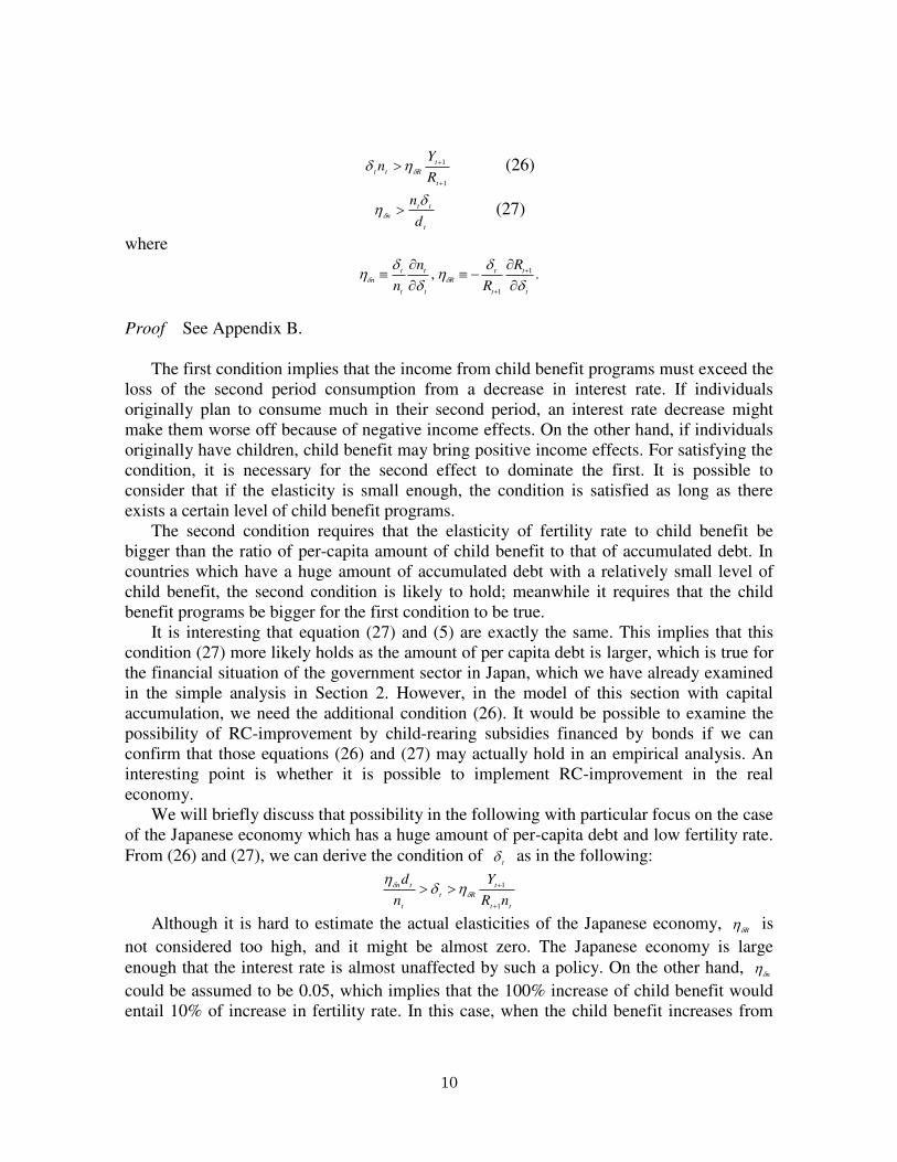
10
1
1
t
t
RttR
Yn (26)
t
tt
nd
n (27)
where
., 1
1 t
t
t
t
R
t
t
t
t
n
R
R
n
n
Proof See Appendix B.
The first condition implies that the income from child benefit programs must exceed the
loss of the second period consumption from a decrease in interest rate. If individuals
originally plan to consume much in their second period, an interest rate decrease might
make them worse off because of negative income effects. On the other hand, if individuals
originally have children, child benefit may bring positive income effects. For satisfying the
condition, it is necessary for the second effect to dominate the first. It is possible to
consider that if the elasticity is small enough, the condition is satisfied as long as there
exists a certain level of child benefit programs.
The second condition requires that the elasticity of fertility rate to child benefit be
bigger than the ratio of per-capita amount of child benefit to that of accumulated debt. In
countries which have a huge amount of accumulated debt with a relatively small level of
child benefit, the second condition is likely to hold; meanwhile it requires that the child
benefit programs be bigger for the first condition to be true.
It is interesting that equation (27) and (5) are exactly the same. This implies that this
condition (27) more likely holds as the amount of per capita debt is larger, which is true for
the financial situation of the government sector in Japan, which we have already examined
in the simple analysis in Section 2. However, in the model of this section with capital
accumulation, we need the additional condition (26). It would be possible to examine the
possibility of RC-improvement by child-rearing subsidies financed by bonds if we can
confirm that those equations (26) and (27) may actually hold in an empirical analysis. An
interesting point is whether it is possible to implement RC-improvement in the real
economy.
We will briefly discuss that possibility in the following with particular focus on the case
of the Japanese economy which has a huge amount of per-capita debt and low fertility rate.
From (26) and (27), we can derive the condition of t
as in the following:
tt
t
Rt
t
tn
nR
Y
n
d
1
1
Although it is hard to estimate the actual elasticities of the Japanese economy, R is
not considered too high, and it might be almost zero. The Japanese economy is large
enough that the interest rate is almost unaffected by such a policy. On the other hand, n
could be assumed to be 0.05, which implies that the 100% increase of child benefit would
entail 10% of increase in fertility rate. In this case, when the child benefit increases from

11
10,000 yen to 20,000 yen every month, the fertility rate might increase from 1.34 to 1.39. If
the debt amount t
d is 20 million yen, then as long as child benefit per child is below 1
million yen, this condition satisfies.
Though the population has not been decreasing dramatically at present, in future it will
decline much more rapidly. In such a case, the per capita amount of debt will increase
dramatically and there would be a greater possibility for RC-improvement.
4.2. Case 2: if 0~ s and 0~ n are satisfied
First we will consider the sign of tt
k /1
.
0~1
1
11
1
1
~
1
~
~
1
~
1
t
t
t
t
t
t
t
t
t
t
t
t
k
R
R
S
tk
R
R
n
t
S
t
n
t
t
kn
kk
(25’)
In this case, we need the conditions for improving efficiency as discussed above.
Proposition 4 RC-improvement is achieved by child benefit with public debt resources
when the following is true:
1
11
1
1
~
~)1(~
~
t
tt
R
tt
tt
WRn
d
n
dR
nW (28)
where
t
t
t
t
t
t
t
t
R
W
W
R
RW
1
1
1
1
,
Proof See Appendix C.
This condition implies that the elasticity of fertility rate to child benefit should be high
enough to dominate the right-hand-side effects. We will consider a small change of t
.
First, when the elasticity of k to is considered to be not too high, it is likely for the
condition to be satisfied. In that case, both R and
W are close to zero, which
renders the right-hand side of (28) also close to zero and facilitates satisfying the condition.
Second, when 1td is increases, the condition becomes more likely to be satisfied, as
shown in Proposition 3. It shows that the possibility to improve efficiency by child benefit
is higher in both cases when the amount of existing debt is huge.
Example 1 We assume specific forms for preferences and production technology in the
above model. Suppose we have preferences:
1
1tttYXnU
and production technology:
.)( ttt
kAkf
Then the sufficient conditions for RC-improvement are
)1)(1(~
11/
t
tt
dz (29)
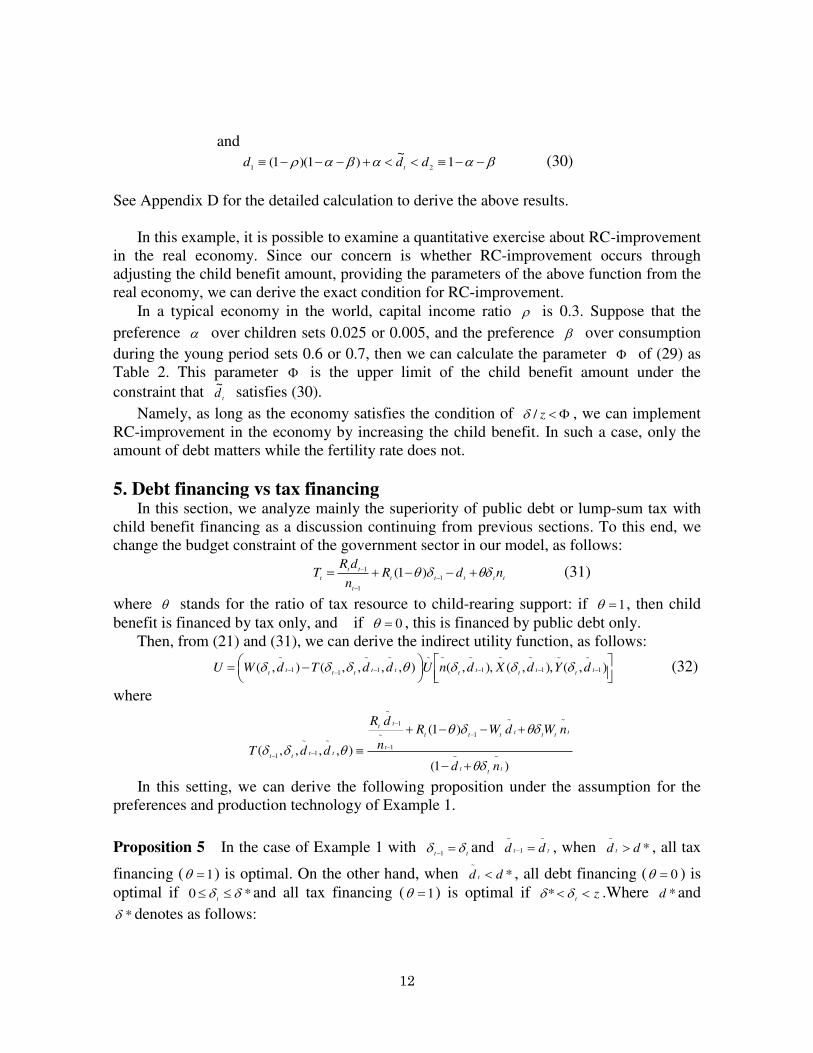
12
and
1~
)1)(1(21
dddt
(30)
See Appendix D for the detailed calculation to derive the above results.
In this example, it is possible to examine a quantitative exercise about RC-improvement
in the real economy. Since our concern is whether RC-improvement occurs through
adjusting the child benefit amount, providing the parameters of the above function from the
real economy, we can derive the exact condition for RC-improvement.
In a typical economy in the world, capital income ratio is 0.3. Suppose that the
preference over children sets 0.025 or 0.005, and the preference over consumption
during the young period sets 0.6 or 0.7, then we can calculate the parameter of (29) as
Table 2. This parameter is the upper limit of the child benefit amount under the
constraint that t
d~
satisfies (30).
Namely, as long as the economy satisfies the condition of z/ , we can implement
RC-improvement in the economy by increasing the child benefit. In such a case, only the
amount of debt matters while the fertility rate does not.
5. Debt financing vs tax financing In this section, we analyze mainly the superiority of public debt or lump-sum tax with
child benefit financing as a discussion continuing from previous sections. To this end, we
change the budget constraint of the government sector in our model, as follows:
ttttt
t
tt
tndR
n
dRT
1
1
1 )1( (31)
where stands for the ratio of tax resource to child-rearing support: if 1 , then child
benefit is financed by tax only, and if 0 , this is financed by public debt only.
Then, from (21) and (31), we can derive the indirect utility function, as follows:
),(),,(),,(),,,,(),( 1
~~
1
~~
1
~~~~
1
~
11
~
ttttttttttttdYdXdnUddTdWU (32)
where
)1(
)1(
),,,,(~~
~~
1
1
~
1
~
~
1
~
1
ttt
ttttttt
t
tt
tttt
nd
nWdWR
n
dR
ddT
In this setting, we can derive the following proposition under the assumption for the
preferences and production technology of Example 1.
Proposition 5 In the case of Example 1 with tt
1and tt dd
~
1
~
, when *~
dd t , all tax
financing ( 1 ) is optimal. On the other hand, when *~
dd t , all debt financing ( 0 ) is
optimal if *0 t
and all tax financing ( 1 ) is optimal if zt * .Where *d and
* denotes as follows:

13
1
1*d
z
d
)1()1)(1(
1*~
Proof See Appendix E.
According to Proposition 5, debt financing is optimal only in the case of *~
dd t . In
addition, the condition that the sign of *d is positive as follows:
01
1
⇔
1
1
(33)
And, to the consumption smoothing during young and old periods, we assume the
following.
Assumption 4 The preference parameters of Example 1 satisfy the following
relationship. 1
⇔ 21
(34)
Then, from the constraint of 0 , (33) and (34), we can derive the following corollary,
as the necessary conditions with regards to debt financing.
Corollary 1 Under Proposition 4 and Assumption 4, the necessary condition that debt
financing is optimal is 3/1 .
Proof First, )1/(1 is derived from (33) and 0 . Next, )1/( is derived
from (33) and (34). Hence, from these relationships, 1)1/(2 holds.
Moreover, we can derive the following proposition and example in the case of tax
financing, as in previous sections.
Proposition 6 RC-improvement is achieved by child benefit with lump-sum tax resources
when the following is true:
Case 1: if ns
t
t
t
Rt
Y
Rn
1
1
1
and tttt
RWnd /~~11 (35)
Case 2: if 0~ s and 0~ n
1
1
~
~
tt
tt
WRn
dR
Wn and
ttttRWnd /~~
11 (36)

14
Proof See Appendix F.
Example 2 We assume the preferences and production technology with Example 1. Then
the sufficient condition for RC-improvement of Proposition 6 is
)1/(1
1~
t
d (37)
See Appendix G for the detailed calculation to derive the above results.
6. Conclusion In this paper, we derive the condition of RC-efficiency in an endogenous population
growth setting. According to this, when the elasticity of interest rate to child benefit policy
is close to zero and there exists a huge amount of accumulated debt, having a certain level
of child benefit programs financed by issuing debt and lump-sum tax is RC-improving.
The weakness of this study is the assumptions we made on the preferences, such as
homogeneity. This study report would be more worthwhile if it were possible to show those
results more generally. We will take over this assignment in a following study.

15
Table 2. Range of Child Benefit with RC-improvement
1) Case 1: 3.0 , 025.0 and 6.0 or 7.0 .
Preference Parameters of Utility Debt Parameters
Upper Limit
of
Child Benefit
1
d~
1d
2d
0.025 0.700 0.275 0.220 0.218 0.275 0.125
0.025 0.700 0.275 0.230 0.218 0.275 0.417
0.025 0.700 0.275 0.240 0.218 0.275 0.563
0.025 0.700 0.275 0.250 0.218 0.275 0.650
0.025 0.700 0.275 0.260 0.218 0.275 0.708
0.025 0.700 0.275 0.270 0.218 0.275 0.750
0.025 0.600 0.375 0.290 0.288 0.375 0.125
0.025 0.600 0.375 0.300 0.288 0.375 0.417
0.025 0.600 0.375 0.310 0.288 0.375 0.563
0.025 0.600 0.375 0.320 0.288 0.375 0.650
0.025 0.600 0.375 0.330 0.288 0.375 0.708
0.025 0.600 0.375 0.340 0.288 0.375 0.750
0.025 0.600 0.375 0.350 0.288 0.375 0.781
0.025 0.600 0.375 0.360 0.288 0.375 0.806
0.025 0.600 0.375 0.370 0.288 0.375 0.825
2) Case 2 : 3.0 , 05.0 and 6.0 or 7.0 .
Preference Parameters of Utility Debt Parameters
Upper Limit
of
Child Benefit
1
d~
1d
2d
0.050 0.700 0.250 0.230 0.225 0.250 0.125
0.050 0.700 0.250 0.240 0.225 0.250 0.300
0.050 0.600 0.350 0.300 0.295 0.350 0.125
0.050 0.600 0.350 0.310 0.295 0.350 0.300
0.050 0.600 0.350 0.320 0.295 0.350 0.417
0.050 0.600 0.350 0.330 0.295 0.350 0.500
0.050 0.600 0.350 0.340 0.295 0.350 0.563

16
Appendix A: Proof of Proposition 2
It is possible to show this with the same logic as Michel and Wigniolle (2007). We will
follow their proof for the most part and change the different points. In equilibrium, the
market adjusts only the capital level, and we do not need to consider a change of . Hence,
for a given sequence of 0
}{tt
, is represented in the following way: ~~~
)](',[)](',[),( dkfzskkfznkz
.
We will show that 0 has a unique solution. In order to show this, we will check the
property of . First, we will check monotonicity of this function. The derivative of the
first term kkkfzn
/))](',[(~
is positive, since )(' kfR is monotonically decreasing in
k and 0~
R
n . The derivative of the second term kkfzs
/)](',[~
is negative, since 0~
R
s .
Hence, is increasing in k .
Next, suppose we have a certain level of child benefit . At this time, when k goes to
0 , it can be bounded in such a way that 1k )1(')(' fkf . Then we obtain the following
inequalities:
)]1(',[)](',[
)]1(',[)](',[~~
~~
fzskfzs
fznkfzn
and thus ~~~
)]1(',[)]1(',[),( dfzskfznkz .
Finally, we have
0)]1(',[),(lim~~
0
dfzskz
k .
When k goes to , we can prove the following by using the contrary thought as
1k )1(')(' fkf . We then obtain the following inequality: ~~~
)]1(',[)]1(',[),( dfzskfznkz .
Thus
),(lim kzk
.
Hence, for any given sequence
0}{
tt , a unique inter-temporal equilibrium
01}{
ttk
exists and the proposition has been proven.

17
Appendix B: Proof of Proposition 3
We will use (25) in the proof. Calculate the change of lifetime utility t
U when the
amount of child benefit t
is raised:
)(~
~
~
~~
~
~~
~
~
)( 1
1
tttt
t
t
t
t
t
t
t
t
t
t
t
t
tttTWU
Y
Y
UX
X
Un
n
UTWU
.~
~
~
~~
~
~~
~
~
)(1
1
1
1
tt
t
t
tt
t
t
t
t
t
t
t
t
t
t
t
t
tttT
WU
Y
Y
UX
X
Un
n
UTWU
It is possible to transform this equation using the household first-order conditions
.~
~1
~~)()(
1
1
1
1
tt
t
t
tt
t
t
tt
t
t
t
ttttT
WU
Y
R
XnzTWU
Moreover, taking derivative of equation (22) with respect tot
, we obtain
t
t
t
t
t
t
t
tt
t
t
t
tY
R
Rn
Y
R
Xnz
~1~~
1~~
)( 1
2
1
1
1
then, by substituting this into the above equation, we have the following equation:
tt
t
t
ttt
t
t
t
ttttT
WUY
R
RnTWU
1
1
1
1
2
1
~~1~)(
(A-1)
where
1
1
11~
1
1
1
~1
1~~
)(1
t
tt
tttttn
R
t
t
t
t
d
dWRdTT t
t
Using this, we can rewrite as
tt
t
t
t
ttttY
R
RnTWU
1
1
2
1
~1~)(
.~1
1~~
~1
1
11~
1
1
t
tt
tttttn
R
t
t
t
d
dWRdWU t
t
This equation represents the effect of the change in child-rearing subsidies }){(0
tt on
lifetime utility of generation t , given a set of debt policies }){(0
tt
d . If the sign of the big
parenthesis of the first term and the coefficient of the second term are both positive, it is
possible to bring welfare improvement to all generations by enlarging child benefit
programs since the sign of t
U~
is positive from homogeneity. Moreover, since 0/1 tt
W
from equation (15) and (25), the latter is always true in the case that the coefficient sign of
the first term is positive. Namely, the sufficient condition of RC-improvement is as follows:
t
t
t
Rt
Y
Rn
1
1
1
(A-2)
where
t
t
t
t
R
R
R
1
1
and

18
0~
1
1~~
1
11~
1
1
tt
tttttn
R
t
t
d
dWRdTt
t
(A-3)
This form (A-3) holds when
0
~
)1(][~
~
111
1
t
tt
WRtRn
tt
ttdW
Rn
dR
0~
~~
)1(~
~
1
1
1
1
t
tt
t
t
WR
t
tt
Rn
d
nd
R
W
d
n
1
1
1
1
~
~~
)1(~
~
t
tt
t
t
WR
t
tt
Rn
d
nd
R
W
d
n
(A-4)
where
t
t
t
tW
WW
1
1
Since 0R and 0
W , we can express in the following form:
11
1
1
11
~
~~
)1(~
~
~
~
t
tt
t
t
WR
t
tt
R
t
tt
d
nd
R
W
d
n
d
n
(A-5)
As a result of (A-2), (A-4) and (A-5), we can get the following sufficient conditions for
RC-improvement:
t
t
t
Rt
Y
Rn
1
1
1
1
11
~
~
t
tt
n
d
n

19
Appendix C: Proof of Proposition 4
We will use (25') in the proof. Calculate the change of lifetime utility t
U when the
amount of child benefit t
is raised, we can use the result already obtained from the
previous section:
tt
t
t
ttt
t
t
t
ttttT
WUY
R
RnTWU
1
1
1
1
2
1
~~1~)(
(B-1)
where
1
1
11~
1
1
1
~1
1~~
)(1
t
tt
tttttn
R
t
t
t
t
d
dWRdTT t
t
Using t
T in the original equation,
tt
t
t
t
ttttY
R
RnTWU
1
1
2
1
~1~)(
1
1
11~
1
~1
1~~
~1
t
tt
tttttn
R
t
t
t
d
dWRdWU t
t
The first term is always positive in this case. We are interested in the sign of the second
term. To have sufficient conditions for improving the utility level, the term should be
positive. Hence,
.0~
1
1~~
1
11~
1
1
tt
ttttn
R
t
t
d
dWRdWt
t
The condition is calculated as in the following:
0~1
1~~
~
~
~
~
1
1
11
1
2
1
1
11
1
1
t
t
t
t
tt
t
t
t
t
t
tt
t
t
t
t
t
t
dd
WR
Rn
n
dRR
n
dW
Cancelling out the term )~
1/(1t
d , we can transform the condition as
0~
~
~
~
~
1
11
1
2
1
1
11
1
1
tt
t
t
t
t
t
tt
t
t
t
t
t
t RRn
n
dRR
n
dW
0~
~
~
~
11
1
11
1
1
ttRn
tt
tt
tt
tt
R
t
t
WRR
n
dR
n
dRW
0)1()(~
~
11
1
1
tRRn
tt
tt
t
t
WR
n
dRW
1
11
1
1
~
~)1(~
~
t
tt
R
tt
tt
WRn
d
n
dR
nW
Hence, the sufficient condition is shown in the following:
1
11
1
1
~
~)1(~
~
t
tt
R
tt
tt
WRn
d
n
dR
nW

20
Appendix D: Calculation of Example 1
The first-order conditions from household optimization are
t
tt
tz
TWn
)(
)(ttt
TWX
).)(1(1 tttt
TWRY
We can normalize for tt
TW :
z
nt
~
t
X~
).1(~
1 tt
RY
Deriving the saving amount as ))(1(
tttTWs
⇒ ).1(~ t
s
Factor prices are ttt
kAW )1(
.1 ttt
kAR
Obtaining the dynamics of k ,
t
t
t dz
k ~11
⇔ )(
~1
1 t
t
tz
dk
where
1~
td . (D-1)
Therefore,
.
~1
1
t
t
tdk
Calculate the elasticities
)~
1)(1()(
1
1
1
1
11
1
11
1
1
t
t
t
t
t
t
tt
tt
t
t
t
t
t
R
d
k
k
k
kA
kA
R
R
)(
)1(
t
t
z
)~
1()(
1
1
1
11
11
1
1
t
t
t
t
t
t
tt
tt
t
t
t
t
t
W
d
k
k
k
kA
kA
W
W
)(t
t
z
2)(
)())/(1()(
t
tt
t
t
t
t
tt
t
t
nz
TW
n
zTW
n
.
t
t
z
We can derive sufficient conditions for RC-improvement
1
11
1
1
~
~)1(~
~
t
tt
R
tt
tt
WRn
d
n
dR
nW

21
⇔ d
n
zd
nz
d
zzz~
~)
)(
)1(1(~
~)(
~11
)()(
)1(
⇔ d
nz
d
nz
d~
~)(~
~)(
~1
)1()1(1
⇔ )(
)()
~1)(1(
~
z
zdd
⇔ )(
)()1)(1(
~
z
zd
⇔
zd
/1
1)1)(1(
~
⇔
zd
/1
1)1)(1(
~
(D-2)
Incidentally, since 0 , 1
~dd is derived from (D-2), where
1d denotes as follows:
)1)(1(1
d (D-3)
Therefore, from (D-1) to (D-3),
)1)(1(~
11/
dz
and
1~
)1)(1(21
ddd

22
Appendix E: Proof of Proposition 5
In the indirect utility function (32), ),,,,(~
1
~
1 tttt
ddT depends on the parameter .
Hence, under the assumption that and ~
d is fixed, we can derive the maximum condition
of (32) as follows:
)1(
)1(
min),,,,(min~~
~~
1
1
~
1
~
~
1
~
1
ttt
ttttttt
t
tt
tttt
nd
nWdWR
n
dR
ddT
(D-1)
To search for the optimal value of (D-1), we analyze the sign of the function /T
using the preferences and production technology of Example 1.
The sign of /T = The sign of
)1(
)1(
log~~
~~
1
1
~
1
~
ttt
ttttttt
t
tt
nd
nWdWR
n
dR
= The sign of
)1()1(
~~
~
~~
1~
1
~
~
1
ttt
tt
tttttt
t
tt
ttttt
nd
n
nWdWR
n
dR
nWR
= The sign of
))1(())(1(~~
1~
1
~
~~
1
~~
tttttt
t
tttttttttttt nWdWR
n
dRnnWRnd
= The sign of
tt
t
ttttt
t
t
tnRddnW~
1~
1
~
1
~1 /
= The sign of
In addition, we can denote as follows in the case with tt
1and tt dd
~
1
~
.
tt
t
tR
n
W
1~
1 (D-2)
⇔ 1
~)()
)(
1()()1()(
Ak
n
Ak
1~~
)(1
)1
()(1
)1(
z
dA
z
zd
A

23
1~
~~
)(1
)1()1)(1()1)(1(
z
dAdzd
(D-3)
Because (D-2) doesn’t depend on the parameter and
)(lim z
, the sign of (D-2)
is determined by the sign of the following value on (D-3). 1
~
~ 1)1)(1()0(
z
dAzd (D-4)
The sign of (D-4) is subject to the following rules:
1) When )1/(1*~
dd , )),0[(0)( zfor .
2) When )1/(1*~
dd , there exists * from (D-3) , then
)*),0[(0)( for or ))*,((0)( zfor
Where * denotes as follows:
z
d
)1()1)(1(
1*~
Therefore, from (D-2), (D-3), and the above rules, we can derive the following rules.
1) When )1/(1*~
dd ,
1 is optimal.
2) When *~
dd , 0 is optimal if *0 and 1 is optimal if z * .

24
Appendix F: Proof of Proposition 6
We will use (25) and (25') in the proof. Calculate the change of lifetime utility t
U
when the amount of child benefit t
is raised, we can use (31) with 1 and the results
already obtained from the previous section:
tt
t
t
ttt
t
t
t
ttttT
WUY
R
RnTWU
1
1
1
1
2
1
~~1~)(
(F-1)
where
t
t
tt
t
t
tt
t
TTT
),(),(1
1
1
1
t
t
ttt
ttttttn
R
t
t
ttt
ttttttn
R
nd
nWdWd
nd
nWdWdt
t
t
t
~~1
~~~
~~1
~~~1
~
1
1
1~
11
t
t
ttt
tttttn
R
t
t
t
ttt
ttttttn
R
nd
dWdWdW
nd
nWdWdt
t
t
t
~~1
)~
1(~~
~~1
~~~1
~
1
1
1~
11
ttt
ttt
ttn
R
t
t
ttt
ttttttn
R
nnd
Wdnd
nWdWd
t
t
t
t
~
)~~1(
~~~1
~~~
2
1~
1
1
1~
1
1
Using t
T in the original equation,
tt
t
t
t
ttttY
R
RnTWU
1
1
2
1
~1~)(1
1
1~
1
~~1
~~~
~
1
t
t
ttt
ttttttn
R
t
t
t
nd
nWdWd
WU
t
t
ttt
ttt
ttn
R
tn
nd
WdU t
t
~
)~~1(
~~
2
1~
1 (F-2)
Case 1: if ns
In this case, we are interested in the sign of all terms of (F-2). For having sufficient
conditions for improving utility level, the terms should be positive. Hence,
0~1~
1
1
2
1
t
t
t
t
tY
R
Rn
, .0
~~1
~~~
1
1~
1
1
t
ttt
ttttttn
R
t
tnd
nWdWd
W
t
t
and
0~
~ 1
1
tt
t
t Wdn
R

25
The condition is calculated in the following:
0~1~
1
1
2
1
t
t
t
t
tY
R
Rn
, .0
~~1
~~~~1~~
~11
1
11
1
1
1
2
1
1
ttt
t
t
t
tt
t
t
t
t
t
t
t
t
t
t
t
t
t
nd
nW
dW
dR
nd
n
n
R
W
and
0~
~ 1
1
tt
t
t Wdn
R
Cancelling out the term )~
1/(1t
d , we can transform the condition as
t
t
t
Rt
Y
Rn
1
1
1
, 0~
~
~
~
11
1
11
1
1
tt
tt
Rn
tt
tt
t
t
Wn
dR
n
dRW
(F-3)
and
0~
~ 1
1
tt
t
t Wdn
R
Since 0R and 0
W , the sufficient condition is shown in the following:
t
t
t
Rt
Y
Rn
1
1
1
and
tt
t
t Wdn
R
1
1
~~
Case 2: if 0~ s and 0~ n
In this case, the first term of (F-2) is always positive. We are interested only in the sign
of the second term and the third term of (F-2). Hence, from (F-3), the sufficient condition is
shown in the following:
1
1
~
~
tt
tt
WRn
dR
Wn
and
tt
t
t Wdn
R
1
1
~~

26
Appendix G: Proof of Example 2
It is possible to transform (36) using the equations of Appendix D.
1
1
~
~
tt
tt
WRn
dR
Wn and
tt
t
t Wdn
R
1
1
~~
⇔ )(
~11
)(~1
)()(
)1(1
1
11
t
t
ttt
t
t
t
t
t zd
zdzzz
and
)(
~11
)(~1
11
1
11
t
t
tt
zd
zd
⇔ )~
1(~
111
ttdd
and )~
1(~
111
ttdd
⇔ )1/(1
1~1
td

27
References ・ Abel, A. B., Mankiw, N. G., Summers, L. H., and Zeckhauser, R. J. (1989), “Assessing
Dynamic Efficiency: Theory and Evidence,” Review of Economics Studies 56(1), pp.
1–20.
・ Becker, G. S. (1960), “An economic analysis of fertility. In: Demographic and
economic change in developed countries,” National Bureau of Economic Research
Conference Series 11, pp. 209–231.
・ Becker, G. S. and Barro, R. J. (1988), “A reformulation of the economic theory of
fertility,” Quarterly Journal Of Economics 103, pp. 1–25.
・ Chakrabarti, R. (1999), “Endogenous fertility and growth in a model with old age
support,” Economic Theory 13, pp. 393–416.
・ Conde-Ruiz, J. I. and Gimenez, E. L. (2002), “Perez-Nievas, M.: Efficiency in an
overlapping generations model with endogenous population,” mimeo.
・ Diamond, P.A. (1965), “National Debt in a Neoclassical Growth Model,” American
Economic Review 55(5), pp. 1126–1150.
・ Eckstein, Z. and Wolpin, K. (1985), “Endogenous fertility and optimal population
size,” Journal of Public Economics 27, pp. 93–106.
・ Golosov, M., Jones, L. E. and Tertilt, M. (2004), “Efficiency with endogenous
population growth,” National Bureau of Economic Research 10231.
・ Michel, P. and Wigniolle, B. (2007), “On Efficient Child Making,” Economic Theory
31(2), pp. 307–326.
・ Nishimura, K. and Zhang, J. (1992), “Pay-as-you-go public pensions with endogenous
fertility,” Journal of Public Economics 48, pp. 239–258.
・ Raut, L. K. and Srinivasan, T. N. (1994), “Dynamics of endogenous growth,”
Economic Theory 4, pp. 777–790.
・ Willis, R. (1973), “A new approach to the economic theory of fertility behavior,”
Journal of Political Economy 81, S14–S64.