child poverty, generational mobility and the one child...

Child Poverty, Investment in Children and Generational Mobility: The Short and Long Term Wellbeing of Children in

Urban China after the One Child Policy

Gordon Anderson and Teng Wah Leo

October 2008

Many thanks for helpful comments are due to seminar participants at the 2007 meetings of the Canadian Economics Association, Halifax, Nova Scotia, to the conference participants at the 2nd

ECINEQ meeting in Berlin, and The International Conference on Experiences and Challenges in Measuring National Income and Wealth in Transition Economies, Beijing, and two perceptive referees.

Abstract

China's One Child Policy (OCP) introduced in 1979 changed fundamentally the nature of both

existing and anticipated marriage arrangements and influenced family formation decisions in

many dimensions especially with respect to the number of and investment in children. The policy

coincided with the Economic Reforms of 1979 and the trend towards greater urbanization, all of

which may have influenced the well being of children. This paper examines the mobility status

consequence of children in urban China since the introduction of the OCP and the economic

reforms using data drawn from urban household surveys in China. The analysis first makes the

comparison between child poverty in Canada, the United Kingdom and urban India, where it was

found that both status and trends of child poverty are very different among the countries, with

children not being over represented in the poverty group in urban China. The extent to which the

policies influenced investment in children is next examined by studying the way in which the

relationship between the educational attainment of children and family characteristics changed

within families formed prior to and after 1979. We found that the impact of household income

and parental educational attainment increased significantly over time, with a positive gender

effect where girls advanced more than boys. Applying new techniques for measuring mobility,

we observe the reduction in intergenerational mobility. This phenomenon is found to be

particularly prevalent in the lower income quantiles reinforcing a dynastic notion of poverty.

Introduction

One of the most controversial and far reaching population control policies in recent history is

China’s One Child Policy (OCP) implemented in 1979 and followed since with some minor

modifications. Directed at China’s large population growth rate, the OCP represented a

considerable intervention in the household choice process, where by fines and various other

forms of coercion families were encouraged to limit the production of offspring. Over the same

period child poverty has been a major issue in western (predominantly urban) societies where it

is strongly associated with single parent family situations (in the United Kingdom children of

lone parents are subject to more than twice the risk of poverty compared to children of couples

(Brewer et. al. (2006a))). Its association with a lack of generational mobility and low investment

in child quality has meant that its eradication has been an overt policy target in both Canada and

the United Kingdom1, where child poverty figures of the order of 1 in 6 and 1 in 4 respectively

have been cited in recent years (as compared to 1 in 10 and 1 in 7 respectively for people in

poverty in the population at large). Though child poverty has not been such a direct policy target

in the United States (where roughly speaking 1 in 5 children are in the poor group as compared

with 1 in 10 households in the population at large) policies promoting generational mobility

(reducing the dependence of child outcomes on parental circumstances) and investment in child

quality (the “No Child Left Behind” for example) have been a policy imperative2. In formalizing

1 Without being very explicit, in 1989 the Canadian House of Commons unanimously resolved to “seek to achieve the goal of eliminating poverty among Canadian children by the year 2000” (to date a little progress has been made, though children are still over-represented in the poverty group). With a similar vagueness in 2000, the British Government vowed to “half child poverty by 2010 and eliminate it by 2020”, and to this end the U.K. government committed £8 billion to child contingent income support in the 1999-2004 period (Brewer et. al. (2006)) and some benefit has accrued, by 2004 the number of children in poverty had fallen by some 700,000 and the child poverty rate was at its lowest since the 1980’s. These heroic intentions were not matched by the United States administration where the policy focus has been more on improving generational mobility (e.g. “Headstart” and “No Child Left Behind”).2 All of this can be seen as an attack on the dynastic nature of poverty (Kanbur and Stiglitz (1989)) wherein children of the poor have a greater likelihood of being members of the poor “club” when they become adults.

the mobility imperative, Roemer (2002) remarked that equal opportunity is “Probably the most

universally supported conception of Justice advanced in societies..”. With roots in recent

egalitarian political philosophy (See Dworkin (1981)) the concept sees differential outcomes as

ethically acceptable when they are the consequence of individual choice and action but not

ethically acceptable when they are the consequence of circumstances beyond the individual’s

control.

The OCP intervention changed fundamentally the nature of both existing and anticipated

marriage arrangements and influenced family formation decisions in many dimensions.

Anderson and Leo (2007), in studying the impact of the policy on family formation construed the

OCP as a rationing policy constraining the quantity (but not the quality) of children and,

following Neary and Roberts (1980) and Deaton (1981), anticipated that the demand equations

for quantity and quality of children would be affected accordingly. Increased positive assortative

pairing of couples was observed as was increased investment in children and, also consistent

with rationing theory, income ceased to be a factor in determining family size though it did

become an increasingly important determining factor in investment in children. Such changes in

family formation behavior may well have had substantial impacts on the short and long term

wellbeing of children both in the context of child poverty, the level of investment in children and

their generational mobility. Substantial economic growth (in part due to the economic reforms

embarked upon at the same time as the OCP (Anderson and Ge (2004))) and rapid urbanization

(Anderson and Ge (2005)) also took place at the same time making it difficult to attribute the

child effects solely to the OCP (though theoretically it can be shown that growth would reduce

the incidence of positive assortative pairing (Anderson and Leo (2007)).

This raises issues, addressed in this research, as to whether or not similar circumstances prevail

with respect to child poverty in urban China as in western societies where it is a matter of such

concern, and whether or not the OCP and Economic Reforms had an influence on investment in

children and generational mobility. The study is confined to urban China for two main reasons.

The western societies with which comparison is being made are predominantly urban societies

(the U.K. urban population is over 90%, Canada’s is over 85%) and the child poverty issue is

predominantly an urban feature in those societies. With respect to China (which is 39%

urbanized according to the 2002 census and 28% urbanized according to Houkou registrations)

the OCP appeared to be considerably more effective in the urban sector. The data are samples of

family cohorts for the years 1987, 1989 and 1991 to 2001 drawn from an urban survey of six

provinces in China, Shaanxi, Jilin, Hubei, Sichuan, Guangdong and Shandong3.

To anticipate some of the results, unlike the western experience, children do not appear to be

over-represented in the poverty group either in terms of families formed before or after the OCP,

indeed the sense in which they are under-represented seems to have strengthened over the period.

However generational mobility does appear to have been substantially reduced over the period, a

consequence perhaps of an increasing dependence upon the status of parents and of their

investment in child quality, especially among the lower quantiles of the income distribution.

Section 1 discusses the empirical strategy and the extent to which the observed changes can be

attributed to the OCP and the economic reforms. In section 2 changes in the nature of child

poverty are examined and compared with changes over a similar period in the U.K., Canada and

urban India. Section 3 considers how increased investments in children in urban China have

3 This dataset was obtained from the National Bureau of Statistics as part of the project on Income Inequality during China's Transition organized by Dwayne Benjamin, Loren Brandt, John Giles and Sangui Wang.

impacted their educational attainment and Section 4 considers the changes in generational

mobility in China over the period. Finally some conclusions are drawn in section 5.

1. Empirical Strategy

As noted in the introduction, the passing of the OCP in 1979 corresponded with the Economics

Reforms of 1979. In so far as the economic growth policies has been successful, both of these

policies could potentially lead to increased investments in children across all socioeconomic

groups, thereby preventing the identification of the true indirect impact of the OCP on parental

investment in children, and its consequent effect on intergenerational mobility, and incidence of

child poverty. In this section, we will briefly discuss the dataset(s) used in our analysis, and the

empirical strategy with which we hope to glean the impact of the OCP on children.

The Chinese dataset is drawn from the household survey from the National Bureau of Statistics

of China for the years 1987, 1989, and 1991 to 2001. In the following section, we will examine

the nature of child poverty in comparison with that of U.K., Canada, and urban India to illustrate

the difference in structure, particularly the falling child poverty incidence among the urban

populace in China. Based on the experience of developing economies such as exemplified by

urban India, economic growth and urbanization is typically associated with increased incidences

of child poverty as the poverty-gap increases. To the extent that the nature and incidence of child

poverty differ between India and China, it may be indicative of the effect that OCP may have had

on the urban populace of China. On the other hand, developed economies such as exemplified by

the U.K. and Canada with the preponderance of social policies that aim at alleviating child

poverty serve as a counterpoint to the effect of the OCP of China. To permit this comparison, we

draw our U.K data from the annual Family Resources Survey, for Canada the Statistics Canada

Survey of Household spending and for India the National Sample Survey rounds 50 and 60 from

the Ministry of Statistics for urban India households.

In making the comparison between the four countries, we utilized Stochastic Dominance

techniques to compare child and adult income size distributions. For this analysis, we used

available comparable sample years from each country, specifically 1987 and 2001 for China,

1996 and 2002 for United Kingdom, 1997 and 2004 for Canada and 1994 and 2004 for India.

Although all the Chinese sample years are after the OCP, we can think of the earliest 1987

sample as composed largely of families formed prior to the introduction of the OCP (particularly

when we consider child and parent income realizations which constrains the sample to families

with adult children) while the 2001 sample (as is clearly the case in each of the successive

samples) as composed largely of families formed after the OCP. It is thus appropriate to address

how we can elicit the effects of the OCP from such a collection of samples.

To understand this mixture of households formed before and after the OCP, first note that as

mentioned above we may expect that the proportion of pre-OCP deciding households to diminish

substantially over time in successive samples. Let the true pre-OCP and post-OCP density

function of income or academic achievement characteristics, x∈[0, x ] , be fpre (x) and gpost (x)

respectively. Next, let the density function of the same characteristics for the 1987 sample be f(x)

such that it is a mixture of the pre-OCP decider households density (fpre (x)) and the post-OCP

decider households density (gpost (x)) in the form αf fpre (x) + (1-αf) gpost (x) where αf is the

proportion of pre-OCP deciding households in the f(.) distribution of 1987. In a similar fashion

let the 2001 sample distribution g(x) be a mixture of the form αg fpre (x) + (1-αg) gpost (x) where αg

is the proportion of pre-OCP deciding households in the g(.) distribution. Furthermore, it is

reasonable to expect αf - αg > 0, that is to say f(x) is largely a household income distribution of

pre-OCP deciders albeit in 1987 and g(x) is largely a household income distribution of post-OCP

deciders in 2001. It is then clear that even if the interest is in the underlying dominance

relationship between fpre (x) and gpost (x), the dominance relationship can still be examined by

considering the mixture of two density functions. To see this note that in considering a

dominance relationship between f(x) corresponding to the adult distribution in 1987 and g(x)

corresponding to the child’s distribution, we have for a k’th order dominance relationship:

∫ ...∬ f x −g x dxdy ... dz=∫ ...∬ f f prex 1− f g post x − g f prex 1−g g post x dxdy ... dz

= f−g ∫ ...∬ f pre x−g post x dxdy ... dz

If household decisions are thought to be made prior to age 25 based on the age of head of

household, αf is approximately 0.8079 and αg is approximately 0.2768 in our samples so that the

1987 comparison will be that of predominantly pre-OCP deciders and the 2001 comparison will

be that of predominantly post-OCP deciders. In so much as the OCP is peculiar to China, the

change in the difference in the dominance relationship as compared to the three other countries

allows us to glean for suggestive evidence that the OCP might have induced it.

To directly examine the changes in investments in children and the evolution of generational

mobility we pooled all the cross-sectional data from 1987, 1989 and 1991 to 2001, and using the

birth year of the mothers, separated the dataset into pre- and post-OCP families. A family is

classified as possibly affected by the OCP (Post-OCP Family) if the mother was younger than 25

years of age at the onset of the OCP, and could have had at most one child by 1979. All other

families are classified as “Pre-OCP Families”, and further to minimize the selection problem due

to truncation of observations within these families which are more likely to experience older

children leaving the household to form their own families, we excluded families whose heads

were born before the 1940's. The first criterion in creating the “Post-OCP Families” was selected

based on the observed age of first birth among the populace, which is summarized in section 3.

The addition of the second criterion is because it is possible that a young women might have

married early, and consequently have had more than one child by the onset of the OCP, that is

her family size choice would not have been subject to the OCP. From this set of families, we

then considered children over 19 and less than 30 inclusive, who can be attached to parents

within the household, since in so doing we can ensure that parental investments in these children

(as realized in their educational attainment) would have been more or less completed. Put

another way, we ignore identifiable relationships between the head of household and their spouse

with other relatives such as parent-in-laws. This is done since it is not possible to link all children

of older members of the household (parent-in-laws) to their children, most of whom may not be

in the same household. We will nonetheless examine the selection problems and their consequent

biases in section 4. Note that although all of the cross sectional data contributed to the pre-OCP

observations, post-OCP observations occur only after 1998.

2. Child Poverty and Wellbeing

In western societies, concern with child poverty pertains to the over-representation of children in

the poverty “club”, alternatively put the children in those societies experience a greater degree of

measured poverty than do the adults. How this poverty “club” is measured has been the subject

of much debate. What should the poverty frontier be? Should incidence, depth or intensity

measures be used? How should adults and children be compared within the context of a

household? To what extent are there returns to scale in household consumption? All are issues

that have received much attention. To this list should be added the question of the household

sharing rule which permits the identification of child and adult income distributions? Thanks to

Atkinson (1987) many of these debates (aside from the last few) may be circumvented by

employing stochastic dominance techniques.

Atkinson’s result, also noted in Foster and Shorrocks (1988), establishes a useful link between

poverty indices and stochastic dominance relations for more general welfare comparisons which

may be summarized as follows. If income distribution FA (x) stochastically dominates income

distribution FC (x) over the interval 0 to x*, x* ≤ x , at a particular order, then all poverty

measures in a specific class will record greater poverty for society C than society A for any

poverty line up to x*. Intensity of poverty measures require dominance of order three or less,

depth of poverty measures require dominance of two or less and incidence measures (e.g.

poverty rates) require dominance of order 1. Noting that dominance of order j implies dominance

of order k for k > j, we see that first order dominance of A over C implies greater poverty in C

than in A for any poverty measure based upon a cut-off less than x*. Thus in the present context,

child FC (x) and adult FA (x) income distributions can be compared and if the former is

stochastically dominated by the latter at all incomes less than x* we can conclude that children

are over-represented in the poverty group regardless of the poverty index used as long as the

poverty cutoff is less than x*.

Child and adult income distribution comparisons, computed on the basis of attributing the

household equivalized income (using the square root rule) to each child or adult in the

household4, are made for the China datasets for the years 1987 and 2001. Similar comparisons

were calculated for the U.K. for 1996 and 2002, Canada for 1997 and 2004 and India for 1994

and 20045. Summary statistics for the comparison distributions are reported in Table 1. Note that

the location measures for the child distributions are greater than the location measures for adult

distributions in China whereas the situation is reversed in the U.K., Canada and India (note that

all comparisons are in within country real terms). Child distributions are always less dispersed

than the corresponding adult distributions in all comparisons. With the exception of the 1987

adult distribution in China, which possesses a much larger standard deviation compared to its

child counterpart, relative variability is pretty stable across distributions.

Table 1: Sample characteristics log adult real equivalized household incomeMean Median Standard Coefficient Sample Deviation of Variation Size

China Child 1987China Adult 1987

4.7819 4.8548 0.6164 0.1289 3387 4.5317 4.8040 1.2556 0.2771 2074

China Child 2001China Adult 2001

8.8374 8.9197 0.8642 0.0978 10569 8.6875 8.7916 0.9050 0.1042 3936

UK Child 1996UK Adult 1996

5.3423 5.3390 0.6380 0.1194 17386 5.5021 5.5277 0.6797 0.1235 60323

UK Child 2002UK Adult 2002

5.5985 5.6089 0.6750 0.1206 9401 5.7257 5.7703 0.7509 0.1311 32691

Canada Child 1997Canada Adult 1997

10.0136 10.0858 0.6685 0.0668 1304010.1234 10.1721 0.6952 0.0687 34594

Canada Child 2004Canada Adult 2004

10.3216 10.3658 0.6746 0.0654 9214 10.3731 10.4193 0.7115 0.0686 26027

India Child 1994India Adult 1994

11.3268 11.2815 0.5446 0.0481 67033 11.4490 11.4012 0.5748 0.0502 141215

India Child 2004India Adult 2004

11.9622 11.9234 0.4811 0.0402 12342 12.0444 11.9996 0.5151 0.0429 13716

4 Comparing child and adult income distributions in this way involves very strong implicit assumptions about the way income is allocated or shared within the family which is fundamentally an unobservable phenomenon. Different sharing rules would produce substantially different outcomes establishing what those rules may be is a matter for ongoing research (see Browning et. al. (2006) for instance). The sensitivity to the “square root rule” choice was checked for the Chinese results. They appear robust for all scaling values between 0.0 and 0.68, thereafter no significant differences between child and adult distributions could be detected 5 The non-China data used in this study relate to United Kingdom household income net of direct taxes drawn from the annual Family Resources Survey , for Canada the Statistics Canada Survey of Household spending and for India National Sample Survey (NSS) rounds 50 and 60 from the Ministry of Statistics for Urban India households.

Diagram 1 illustrates the comparisons of the distributions. It is readily seen that for 2001 at every

decile cut-off up to the 9th there were smaller proportions of children in the group than there were

adults, very much a property of the child’s income distribution first order dominating that of the

adults. Thus we can safely conclude that for almost any poverty measure at any cutoff line child

poverty would be less than adult poverty. The same is almost true for the 1987 year where the

proportion of children is always less than the proportion of adults for every decile cut-off up to

the 7th, so that child poverty would be less than adult poverty for any poverty line up to the 7th

decile for virtually all poverty measures. Actually 1st order dominance would be rejected over the

whole income range since for the 8th and 9th deciles child shares are significantly greater than

adult shares but second order dominance of the adult income distribution by the child’s

distribution would prevail (see appendix 1 for details) so that all depth and intensity poverty

measures would record less poverty for children than for adults over the whole income range.

Diagrams 1a, 1b and 1c illustrate the corresponding comparisons for the selected years for

Canada, the U.K. and India respectively. Notice that for the U.K. and India comparators the

reverse is true, at every decile cut-off up to the 9th the child’s income share is greater than the

adult’s (both in 1996 and 2002), very much a characteristic of the adult income distribution

stochastically dominating the child’s income distribution at all orders indicating an over-

representation of children in the poverty group however defined. The same is true for Canada

except for the 2nd decile in the 2004 comparison (but this difference is not significantly different

from 0 and not enough to contradict the same dominance result as for the U.K. and India).

Diagram 1

Diagram 1a

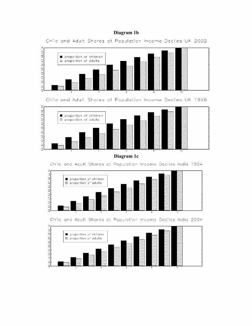
Diagram 1b

Diagram 1c

In essence the comparisons which permitted such strong and sweeping statements to be made

were of the form:

∫0

x FCi z −F A

i zdz≤0∀ x

where F Hi ' x =∫0

xF H

i z dz , i '=i1 and F H0 z = f H z for H=A,C and i={1,2, ...} . These are

conditions under which we can infer that society C is better off than society A. Thus from the

above, for China it may be inferred that the society of children were better of than the society of

adults for all utilitarian social welfare functions in 2001 and for all social welfare functions that

express a preference for mean preserving progressive transfers in 1987. The reverse is true for

the U.K., Canada and India in both their respective comparison periods and the society of adults

is better off than the society of children in terms of all utilitarian social welfare functions.

However we can take the analysis further, consider the income distribution of society H in year k

to be FH,k (x) and consider the condition:

∫0

x F C , 2001i −F A , 2001

i − FC ,1987i −F A,1987

i dz≤0,∀ x , i∈{1,2,. ..}

This responds to the question: “Does the extent to which the child’s society was better off than

the adult's in 2001 dominate the extent to which the child’s society was better off than the adult’s

in1987?”. This is essentially a difference in dominance comparison, part of the toolkit for

studying polarization (Anderson (2004)). The comparison results employing the Wolak (1989)

method for comparing multivariate inequalities are reported in Table 2 for China 2001 and 1987,

for Canada 2004 and 1997, for the UK 2002 and 1996 and for India 2004 and 1994.

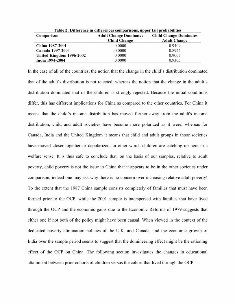
Table 2: Difference in differences comparisons, upper tail probabilitiesComparison Adult Change Dominates

Child ChangeChild Change Dominates

Adult ChangeChina 1987-2001 0.0000 0.9409Canada 1997-2004 0.0000 0.8925United Kingdom 1996-2002 0.0000 0.9007India 1994-2004 0.0000 0.9305

In the case of all of the countries, the notion that the change in the child’s distribution dominated

that of the adult’s distribution is not rejected, whereas the notion that the change in the adult’s

distribution dominated that of the children is strongly rejected. Because the initial conditions

differ, this has different implications for China as compared to the other countries. For China it

means that the child’s income distribution has moved further away from the adult's income

distribution, child and adult societies have become more polarized as it were, whereas for

Canada, India and the United Kingdom it means that child and adult groups in those societies

have moved closer together or depolarized, in other words children are catching up here in a

welfare sense. It is thus safe to conclude that, on the basis of our samples, relative to adult

poverty, child poverty is not the issue in China that it appears to be in the other societies under

comparison, indeed one may ask why there is no concern over increasing relative adult poverty!

To the extent that the 1987 China sample consists completely of families that must have been

formed prior to the OCP, while the 2001 sample is interspersed with families that have lived

through the OCP and the economic gains due to the Economic Reforms of 1979 suggests that

either one if not both of the policy might have been causal. When viewed in the context of the

dedicated poverty elimination policies of the U.K. and Canada, and the economic growth of

India over the sample period seems to suggest that the domineering effect might be the rationing

effect of the OCP on China. The following section investigates the changes in educational

attainment between prior cohorts of children versus the cohort that lived through the OCP.

3. Investment in Children

One feature of the OCP impact on family formation noted in Anderson and Leo (2007) is the

increased investment in child quality. To illustrate the issue here, investment in children as

reflected in their educational attainments is examined. As noted in section 1, for comparison

purposes only children between the ages of 19 and 30 are studied so that the parental aspect of

the investment activity may assume to have been completed and cohorts of such children were

derived from all samples from 1987, 1989 and 1991 to 2001, and for all six provinces, separating

the samples into pre-OCP families consisting of mothers who were 25 years old and older in

1979 (including also younger mothers who had more than 1 child by 1979 since the OCP would

not have been binding on them), and post-OCP families with mothers who were younger than 25

in 1979 (with at most one child by 1979).

The summary of some of the variables are reported in table 3. Note that both groups have very

similar age at first birth among the mothers in both pre- and post-OCP cohorts, and the

substantially lower number of children per family after the OCP. In addition, despite the fact that

pre-OCP parents being more advanced in their careers, the average deflated and equivalized6

incomes of pre-OCP parents are all lower than their post-OCP counterparts, this in spite the fact

that post-OCP fathers had marginally lower educational attainment, while post-OCP mothers had

higher educational attainment compared to the pre-OCP cohort. This is likely due to the

increased positive assortative matching and lower marriage rates noted in Anderson and Leo

(2007).

6 Deflated as suggested by Brandt and Holz (2006).

Table 3: Summary of Individual and Household Characteristics Variables Pre-OCP Post-OCP

Mother's Age at First Birth 25.77 24.38

(3.17) (1.7)

Father's Age at First Birth 29.08 27.07

(3.89) (2.54)

Age 21.97 19.61

(2.48) (0.79)

Proportion Female 0.46 0.51

Educational Attainment 3.45 3.54

(1.07) (1.02)

Birth Order 1.42 1.14

(0.62) (0.38)

Family Size 3.91 3.35

(0.81) (0.6)

Deflated & Equivalized Father's Income ('000s)

2.22 2.79

(2.04) (2.98)

Deflated & Equivalized Mother's Income ('000s)

1.56 1.93

(1.55) (2.17)

Father's Education 3.04 2.95

(1.37) (1.24)

Mother's Education 2.44 2.6

(1.24) (1)

Father's Age 51.75 46.73

(4.6) (2.62)

Mother's Age 48.44 44.04

(3.78) (1.67)

Number of Children 1.83 1.26

(0.75) (0.51)

Number of Observations 11154 492

Note: 1. Standard Deviations in parenthesis and median in brackets.2. Educational attainment is measured as an integer indexed from 0 to 5 with 5 = college graduates

and above, 4 = technical secondary school, 3 = high school, 2 = middle school, 1 = primary school and lower.

Table 4 reports the results of the stochastic dominance comparisons of educational attainment

between the pre- and post-OCP cohorts of children. The first two rows under each attainment

reports the cumulative distribution (First Order Stochastic Dominance) up to the educational

measure, while the third and fourth rows reports the second order stochastic dominance statistics.

It is clear that the post-OCP cohort first order stochasticially dominates the pre-OCP cohort at all

levels of educational attainment suggesting there were indeed significant gains in child

attainment.

Table 4: Stochastic Dominance Test between Pre- and Post OCP Cohorts

Educational Attainment

Pre-OCP Post-OCP Difference

Primary or Less 0.0120 0.0000 0.0120

(0.0010) (0.0000) [1.0000]

0.0120 0.0000 0.0120

(0.0010) (0.0000) [1.0000]

Middle School 0.1807 0.1301 0.0507

(0.0036) (0.0152) [0.9994]

0.9037 0.6504 0.2533

(0.0076) (0.0303) [1.0000]

High School 0.5993 0.5854 0.0139

(0.0046) (0.0222) [0.7297]

8.3895 8.1951 0.1943

(0.0182) (0.0817) [0.9899]

Technical School 0.7554 0.7398 0.0156

(0.0041) (0.0198) [0.7799]

22.6630 22.1950 0.4676

(0.0313) (0.1465) [0.9991]

Note: 1. Standard errors are in parenthesis, and p-values are in brackets. 2. The first two rows for each educational attainment level are for first order stochastic dominance comparisons while the third and fourth rows are for second order stochastic dominance comparisons.

To examine the determinants of child quality, educational attainment is regressed upon the

logarithm of total parental equivalized income, father’s and mother’s educational status,

household size (including all members of the extended family), and the gender of the child (1 if

female, 0 otherwise) and birth order (representing the order in which the child arrived in the

family, 1 = first child, 2 = second child…). Family consumption deflated (Brandt and Holz

(2006)) income equivalization is based upon the square root rule (Brady and Barber (1948))

under which family income is divided by the square root of the number of persons in the family

(as opposed to the household) and reflects returns to scale in family consumption. Parental

educational status is included to reflect both inherited abilities and parental preferences,

household size is included independently of family income to reflect investment scale effects

beyond the consumption nexus. Gender and birth order effects are included following Bjorklund

et. al (2004) and Kantarevic and Mechoulan (2006).

Table 5 reports regressions for the pre-OCP and post-OCP cohorts which were performed for

single child, and two child family situations7. Examining single child families in both panel A

and B, note the great similarity for both the pre- and post-OCP families in the effect parental

income and father's educational attainment has on child educational attainment. Despite the

differences due to household size, and the effect of the child being female (both of which are not

statistically significant), there is in fact no difference in the “production technology” between the

two cohorts. This however is not surprising since the choice of investment is predicated on the

same number of children, consequently whether that choice is exogenously imposed or

independently chosen, there should be no difference in the effect on investment.

7 Although there were sufficient observations to examine the production technology of families with more than 2 children in the pre-OCP state, this family structure is rare in the post-OCP state, and consequently has been left out of our analysis.

Table 5: Child Educational Attainment Regressions

Panel A: Pre-OCP 1 Child Families 2 Child Families

Deflated & Equivalized Family Income 0.3472 0.2964

(0.0351) (0.0282)


(0.0128) (0.0105)


(0.0140) (0.0120)

Household Size 0.0225 0.0633

(0.0524) (0.0468)

Female 0.1004 0.0890

(0.0308) (0.0260)

Birth Order 0.0452

(0.0259)

Parental Cohort Dummies Yes Yes

Provincial & Year Dummies Yes Yes

R2 0.2122 0.2085

σ 0.9516 0.9488


Panel B: Post-OCP 1 Child Families 2 Child Families

Deflated & Equivalized Family Income 0.3022 0.5827

(0.0850) (0.1966)


(0.0467) (0.0711)


(0.0580) (0.0883)

Household Size -0.1636 -0.9707

(0.1231) (0.6185)

Female 0.0853 0.3971

(0.0987) (0.1715)

Birth Order -0.2387

(0.1680)

Parental Cohort Dummies Yes Yes

Provincial & Year Dummies Yes Yes

R2 0.2138 0.4333

σ 0.9368 0.7701


Test of Difference, F Statistic [p-value] 0.1562 [1.0000] 1.4415 [0.1126]

Standard Errors are in parenthesis, and p-values are in brackets.

On the other hand, comparing families with two children, note the significant increase in the

income effect (doubling from approximately 29 percentage point to 58 percentage point) and the

paternal effect on educational attainment in their children, while the maternal effect waned. In

addition, note the significant increase in the female effect, suggesting greater investments were

placed with female children among these families. Although birth order was positive among pre-

OCP cohorts, this changed sign among post-OCP children. Despite these differences, test of the

restriction that all the coefficients for both pre- and post-OCP cohorts are the same cannot be

rejected.

A possible reason for the stronger connection in income and paternal educational attainment

among families with more than one child is that the former is a prerequisite to circumvent the

OCP, thereby creating the significant differential between the pre- and post-OCP cohorts. In so

far as the primary determinant of family income is dependent on paternal labour supply, the

increase in paternal educational effect is likewise then not surprising. However, given the

concurrent effects of the Economic Reforms, the former argument may not be binding without

the economic growth that was generated. With respect to the increase in female effect, it is

possible that it is a reaction to marriage market sex ratio (see table 3) so as to enhance the

probability of a good spousal match for their daughters and personal wealth through the labour

market (Peters and Siow (2002)).

4. Generational Mobility

Greater parental investments in child quality undoubtedly strengthen the ties between

generational income distributions, making it more likely that parents with high (low) incomes

will have children who will earn high (low) incomes when they become adults. This increased

dependence between child and parent outcomes constitutes a reduction generational mobility.

Here the generational mobility phenomenon is examined by studying the dependence between

parent incomes and educational attainments and child educational attainments.

Mobility has mostly been studied in the context of intergenerational income transitions (see

Corak (2004, 2006) for a survey and examples) generally assessed via the regression coefficient

(β) of the child income (y) on the corresponding parent income (x) inferring mobility (equal

opportunity) as β→0 and immobility (unequal opportunity) as β→1. However mobility

interpretations of β are limited by its connection to the correlation coefficient ρyx (β = ρyx(σy /σx)),

and its ability to reflect dependence. In addition, it is constrained by the implicit assumption that

y and x are homogeneously linear across all socioeconomic strata8. However if the degree of

dependence is the issue and the setting is not homogeneous, the transition matrix between the

common quantiles of the marginal densities f(x) and g(y) can be more informative. This has

given rise to the application of techniques derived from Markov Chain processes and the

development of mobility indices, some based upon the nature of the transition matrix directly

(with complete mobility the columns of a transition matrix are identical), some based upon other

related concepts9. When the quantiles or categories of f(x) and f(y) match or are common, such an

analysis is straightforward, but there are significant difficulties when they are not. Here, since the

8 As an index β would not prove very effective if immobility were just confined to the lowest income group for example. Indeed there are dangers with interpreting zero correlation with perfect mobility, imagine a deterministic world (perfectly immobile) where below a certain parental income there is an exact negative relationship between parent and child outcomes whereas above that income there is an exact positive relationship between parent and child outcomes, an appropriately balanced sample would yield 0 correlation with an inferred perfect mobility for what is a completely deterministic and immobile state.9 Bartholemew (1982), Blanden et. al. (2004), Chakravaty (1995), Dearden et. al. (1997), Hart (1983), Maasoumi (1986), Maasoumi and Zandvakili (1986), Prais (1955), Shorrocks (1976), (1978) have all produced “Transition” based mobility indices many of which are discussed in Maasoumi (1995)).

data does not present in terms of the common quantiles of two single variables, we consider

more general transition processes between generations characterized by different sets of

characteristics which do not readily lend themselves to a Markov chain interpretation.

Following Anderson, Ge and Leo (2008) and Anderson and Leo (2006) the extent to which

independence accords with the data can be indexed by an overlap measure given by:

OV=∑i∑ j min {p i , jo , pi , j

e }

where p i , jo corresponds to the i,jth cell probability of the observed joint probability matrix and

p i , je corresponds to the i,jth cell probability of the expected joint probability under the null

hypothesis of independence where i corresponds to the ith child characteristic configuration and j

corresponds to the jth parental characteristic configuration. This measure forms a very natural

index since it reflects the proximity of the data to the hypothesis of interest, which is that child

characteristic realization is independent of parental characteristic(s). When the data completely

conform to the hypothesis of interest (in this case independence) OV = 1, otherwise 0 ≤ OV < 1.

OV is easily calculated, p i , jo is simply estimated from the observed cell sample proportions and

p i , je is estimated from the product of the corresponding empirical marginal proportions. An

attractive feature of this index is that they can be readily applied when the underlying parent

child transition matrices are not square and transitions are between multivariate environments.

For example given continuously measured parental characteristics w and x with joint density

f(w,x) and continuously measured child characteristics y and z with joint density g(y,z) and a joint

density of all characteristics given by h(w,x,y,z), then OV estimates the magnitude

∫∫∫∫min[h(w,x,y,z),(f(w,x)g(y,z))]dwdxdydz. In addition they are asymptotically normal sampling

distributions (See Anderson, Ge and Leo (2008)), conveniently facilitating inferences about

trends toward or away from independence over time. Further, these indices can be more focused,

concentrating on a subset of cells that relate to particular features of interest. So for example

mobility amongst the poor could be examined by specifying a null in which only independence

with respect to the poor is entertained so that the mobility of the ith subgroup can be considered

in terms of:

OV i=∑ j∈{1, K }min {

pi , j

pi, p j}

where pi and pj are marginal row and column probabilities respectively10.

To study the impact on generational mobility due to the OCP, we examine the changes in the

degree of dependence between parent and child characteristics pre- and post-OCP. The samples

used are as that in section 3, and parental characteristics considered are family income and

parental educational attainment (the maximum of the parent’s attainments), while the child’s

characteristics are their educational attainments. As before in section 3, only children between

the ages of 19 and 30 residing with their parents were considered so as to allow for them to have

completed their education. In addition to overall parent-child mobility, mobility by gender and

birth order of child are considered following Bjorkland et.al. (2004). Both univariate (Parent

Achievement-Child Achievement and Parent Income-Child Achievement), multivariate indices

(Parent Achievement and Income-Child Achievement) are employed and are reported in table 6.

Examining first panel A, it is clear that in the education-education comparison, as well as the

multivariate comparison reveals a diminished level of mobility, while the slight increase in

mobility for the income-education comparison is not statistically significant, suggesting that the

10 This possibility calls for a concept of “Qualified Equal Opportunity” or “Conditional Mobility” which has been developed elsewhere (Anderson, Leo and Muelhaupt (2008)).

improvement is driven by parental educational attainment, which may be interpreted as non-

pecuniary inheritance.

Table 6: Mobility Differences Pre- and Post- OCP families

Panel A: Mobility of All Children

Pre-OCP Families Post-OCP Families Difference

Mobility-All Children, Education-Education

0.8796 0.8463 0.0334(0.0031) (0.0163) [0.0439]

Mobility-All Children, Income-Education

0.8706 0.8899 -0.0193

( 0.0032) (0.0141) [0.1829]

Mobility-All Children, Education-Income-Education

0.8069 0.7460 0.0607

( 0.0037) (0.0196) [0.0023]

No. of Observations 11154 492

Panel B: Mobility of Male Children


Mobility-Male Children,Education-Education

0.8882 0.8547 0.0335( 0.0041) (0.0227) [0.1459]

Mobility-Male Children,Income-Education

0.8715 0.8688 0.0027

( 0.0043) (0.0217) [0.9026]

Mobility-Male Children,Education-Income-Education

0.8091 0.7289 0.0802

( 0.0051) (0.0286) [0.0057]


Panel C: Mobility of Female Children


Mobility-Female Children, Education-Education

0.8593 0.7986 0.0608(0.0048) (0.0254) [0.0186]

Mobility-Female Children, Income-Education

0.8631 0.8787 -0.0156

( 0.0048) (0.0206) [0.4609]

Mobility-Female Children,Education-Income-Education

0.7905 0.6979 0.0926

(0.0057) (0.0290) [0.0017]


Table 6 Cont'd: Mobility Differences Pre- and Post- OCP families

Panel D: Mobility of 1st Born Pre-OCP Families Post-OCP Families Difference

Mobility-1st Born,Education-Education

0.8769 0.8574 0.0195(0.0039) (0.0169) [0.2620]

Mobility-1st Born, Income-Education

0.8669 0.8877 -0.0208

( 0.0040) (0.0153) [0.1880]

Mobility-1st Born,Education-Income-Education

0.7973 0.7469 0.0504

( 0.0047) (0.0211) [0.0196]


Panel E: Mobility of 2nd Born Pre-OCP Families Post-OCP Families Difference

Mobility-2nd Born,Education-Education

0.8768 0.7227 0.1541

( 0.0057) (0.0569) [0.0070]Mobility-2nd Born,Income-Education

0.8866 0.8013 0.0854

( 0.0055) (0.0507) [0.0941]

Mobility-2nd Born,Education-Income-Education

0.8151 0.5427 0.2724

( 0.0068) (0.0633) [0.0000]


Note: Standard Errors are in parenthesis, and p-values are in brackets.

Panels B and C reports the same tests but by the gender of the child. It is interesting to note that

the decrease in mobility among male children seems to be driven by parental income while that

for female children was through parental educational attainment. To the extent that the pattern

exhibited by female children parallels that when all children all aggregated together suggests that

the decrease in mobility is driven by parental investment in them, which is similar to the insight

gained from the regressions of table 5. Panels D and E reports the same results but differentiating

the order of birth of the child. Both of the univariate tests suggests little difference between first

born child, while there was significant decline in mobility among second born children, results

that parallel that observed among families with one children in table 5. Further, notice that the

improvement among second born children is derived from both parental education and income,

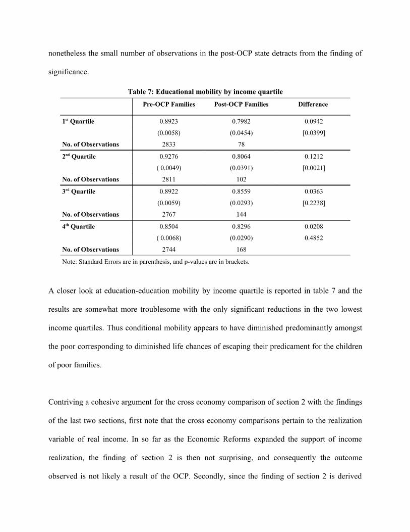
nonetheless the small number of observations in the post-OCP state detracts from the finding of

significance.

Table 7: Educational mobility by income quartile


1st Quartile 0.8923 0.7982 0.0942

(0.0058) (0.0454) [0.0399]


2nd Quartile 0.9276 0.8064 0.1212

( 0.0049) (0.0391) [0.0021]


3rd Quartile 0.8922 0.8559 0.0363

(0.0059) (0.0293) [0.2238]


4th Quartile 0.8504 0.8296 0.0208

( 0.0068) (0.0290) 0.4852


Note: Standard Errors are in parenthesis, and p-values are in brackets.

A closer look at education-education mobility by income quartile is reported in table 7 and the

results are somewhat more troublesome with the only significant reductions in the two lowest

income quartiles. Thus conditional mobility appears to have diminished predominantly amongst

the poor corresponding to diminished life chances of escaping their predicament for the children

of poor families.

Contriving a cohesive argument for the cross economy comparison of section 2 with the findings

of the last two sections, first note that the cross economy comparisons pertain to the realization

variable of real income. In so far as the Economic Reforms expanded the support of income

realization, the finding of section 2 is then not surprising, and consequently the outcome

observed is not likely a result of the OCP. Secondly, since the finding of section 2 is derived

from income and not educational attainment, it does not necessarily contradict the finding of

sections 3 and 4. Since the choice of education is conditional to some degree on the income

commiserating with that qualification, the increase in the support of income at all levels of

educational attainment suggests that using differing variables yields different mobility

conclusions. Our choice of educational attainment is motivated by the idea that it is a better

measure of the permanent income of an individual. Thus income obscures the fact that there is a

fall in mobility among the general populace in post-1979 China, and particularly among the

lower strata of the society, highlighting the increased polarization in contemporary urban China.

Finally, what may be construed as an effect of the OCP is the increase in investment among

female children given the sex ratio in the marriage market created by the binding constraint

presented by the OCP.

In the above examination, we have focused on identifiable family relationships, and particularly

of families with children between the ages of 19 to 30 and who still remain with the family. In

choosing parents who are identified as heads of households, we neglect families embedded in

households under other relationships. To the extent that these missing parents or adults within

the same age range of parents and children of families under examination likewise exhibit

distinct transmission relationships vis-a-vis their children opposing to the reported pattern, our

results may be biased. It is not possible for us to identify these relationships since all

relationships are linked directly to the head of household, but we can nonetheless examine how

different these other individuals are as compared to those included in the sample. This is

informative to the extent that if we are willing to assume that the non-identifiable parents are

representative of the non-identifiable children, we can see how including these other “families”

would increase weight towards a particular educational attainment group or socioeconomic

group, and how it might possibly affect our conclusion. We create these comparison groups

using the year of birth of the individuals and their relationships to the head of household, and

examined if their densities are similar to those used, as well as examine the stochastic dominance

relationships against the sample11.

Although there are distinct differences in the densities of those included in the sample and their

excluded peers (excluded due to the inability to identify their family relationships directly), in

terms of educational attainment the pre-OCP group of parents used first order dominates their

peers, while for the post-OCP parents there does not seem to be a distinct first or second order

dominance relationship. In terms of income, both pre- and post-OCP parents first order dominate

their peers, and this dominance relationship is stronger among post-OCP parents for cutoffs

above the 4th decile. On the other hand, while there does not seem to be a distinct dominance

relationship between pre-OCP children and their peers, post-OCP children first order dominate

their peers not in the sample, suggesting that their inclusion might dilute the educational

transmission effect observed. Taken together, the “missing pre-OCP families” would have

diminished the intergenerational mobility measure for the pre-OCP cohort, while the “missing

post-OCP families” might have accentuated the lack of mobility among the lower

socioeconomic groups. None of which would have altered the substance of our conclusion.

5. Conclusions

Unlike countries in the west, children do not appear to be over-represented in the poverty group

in Urban China in any of the observation periods. What may be interpreted as the child’s income 11 The results of been omitted due to space constraints, but are available from the authors upon request.

distribution is seen to stochastically dominate the adult income distribution predominantly based

households formed in the pre-1979 environment at the second order. The post-1979 era result is

even stronger with the child income distribution first order dominating that of the adult

distribution. Indeed it appears that the two policies of 1979 seem to have polarized (i.e. widened

the gap between) child and adult income distributions12. Thus the general dominance relationship

between child and adult income distributions does not appear to be a result of the OCP13 though

not surprisingly it does appear to have precipitated an improvement in the wellbeing of children

relative to the adult population.

With respect to mobility, the increased intensity of investment in child quality brought about by

the OCP and the Economic Reforms has reinforced the link between parent and child quality and

reduced generational mobility as a result. This is contrary to the results found for the U.S. for

example where generational mobility has increased over the last part of the 20th Century

(Anderson and Leo (2006a)). When viewed by income quartile, increases in immobility are

found to be more prevalent in the lower income quartiles reinforcing notions of “Dynastic

Poverty” discussed in Kanbur and Stiglitz (1986).

12 On the other hand policies pursued in Canada, the UK and India, our comparator societies, appeared to have narrowed the gap between the child and adult income distributions where generally the adult income distribution dominates that of the children.13 It could well be a consequence of the nature of household formation and the extended family found in China (however it does not seem to be the case in Urban India where similar extended family arrangements prevail) together with higher income elasticities of demand for children than are prevalent in the west, all of which is the subject of ongoing research.

References

Anderson G.J. (2004) “Toward an Empirical Analysis of Polarization” Journal of Econometrics 122 1-26.

Anderson G., and Y. Ge (2004) “Do Economic Reforms Accelerate Urban Growth: The Case of China” (2004) Urban Studies 11 2197-2210.

Anderson G., and Y. Ge (2005) “The Distribution of Chinese City Sizes” Journal of Regional Science and Urban Economics

Anderson G.J., Ge Y. and T.W. Leo (2008) “Distributional Overlap: Simple, Multivariate, Parametric and Non-Parametric Tests for Alienation, Convergence and General Distributional Difference Issues”, Mimeo University of Toronto, Department of Economics.

Anderson G.J. and T.W. Leo (2006) “Indices and Tests for Matching and Mobility Theories: A Note” Mimeo University of Toronto, Department of Economics.

Anderson G.J. and T.W. Leo (2006a) “Evaluating Equal Opportunity Policies: The Impact of Changes in Child Custody Law and Practice on Generational Mobility in the United States.” Mimeo University of Toronto, Department of Economics. Anderson G.J. and T.W. Leo (2007) “Family Formation and the One Child Policy in Urban China” Mimeo University of Toronto, Department of Economics.

Anderson G.J, Leo T.W. and R. Muelhaupt (2008) “Qualified Equal Opportunity and Conditional Mobility: The case of Gender Equity in Educational Attainment in Canada.” Mimeo University of Toronto, Department of Economics. Atkinson A.B. (1987) “On the Measurement of Poverty” Econometrica 55, 749-764.

Bartholemew D.J. (1982) Stochastic Models for Social Processes. 3rd ed., Wiley New York.

Bjorklund A., T. Eriksson, M. Jantti, O. Raaum and E. Osterbacka (2004) “Family Structure and Labor Market Success: the Influence of Siblings and |Birth Order on the Earnings of Young Adults in Norway, Finland and Sweden. Chapter 9 in Generational Income Mobility in North America and Europe Miles Corak ed. Cambridge

Blanden, J., A. Goodman, P. Gregg and S. Machin (2004) “Changes in Intergenerational Mobility in Britain” chapter 6 of M. Corak (editor) Generational Income Mobility in North America and Europe. Cambridge

Brady D.S. and H.A. Barber (1948) “The Pattern of Food Expenditures” Review of Economics and Statistics 30 198-206.

Brandt L and C Holz (2006) "Spatial Price Differences in China: Estimates and Implications." Economic Development and Cultural Change, 55 43-86

Brewer M., Brown J. and H. Sutherland (2006) “Micro-simulating Child Poverty in 2010 and 2020” Joseph Rowntree Foundation.

Brewer M., Goodman A., Shaw J., and L. Sibieta (2006a) Poverty and Inequality in Britain: 2006. The Institute For Fiscal Studies.

Browning M., Chiappori P.A., and A Lewbel (2006) “Estimating Consumption Economies of Scale, Adult Equivalence Scales and Household Bargaining Power: Oxford University Economics Department Discussion Paper ISSN 1471-0498.

Chakravarty S.R. (1995) “A Note on the Measurement of Mobility” Economics Letters 48 33 – 36.

Clark, C. (1961) “The Greatest of a Finite Set of Random Variables” Operations Research 9 145-162.

Corak M. (2004) Generational Income Mobility in North America and Europe Cambridge University Press.

Daganzo C. (1980) Multinomial Probit. New York; Academic.

Davidson, R and J-Y Duclos (2000) “Statistical Inference for Stochastic Dominance and for the Measurement of Poverty and Inequality” Econometrica 68, 2000, 1435-1464

Deaton A.S. (1981) “Theoretical and Empirical Approaches to Consumer Demand Under Rationing.” In Essays in the Theory and Measurement of Consumer Behaviour: In Honour of Sir Richard Stone. A.S. Deaton ed. Cambridge University Press.

Dworkin R. (1981) “What is Equality? Part 2: Equality of Resources” Philosophy and Public Affairs 10 283-345.

Foster J.E. and A.F. Shorrocks (1988) "Poverty Orderings" Econometrica 56 pp.173-177.

Hart, P.E. (1983) “The size mobility of Earnings” Oxford Bulletin Of Economics and Statistics 45 181-193.

Kanbur S.M.R. and J.E. Stiglitz (1986) Intergenerational Mobility and Dynastic Inequality Woodrow Wilson Discussion Paper No 111 Princeton University.

Kantarevic J. and S. Mechoulan, (2006) “Birth Order, Educational Attainment and Earnings: an Investigation using the PSID”, Journal of Human Resources 41 (4) 755–777.

Maasoumi E. (1986) “The Measurement and Decomposition of Earnings Mobility” Econometrica 54 991-997

Maasoumi E. (1996) “On Mobility” in D. Giles and A. Ullah (eds) Handbook of Applied Economic Statistics, Marcel Dekker.

Maasoumi E. and S. Zandvakili (1996) “A Class of Generalized Measures of Mobility with Applications” Economics Letters 22, 97-102.

Neary J.P. and K.W.S. Roberts (1980) “The Theory of Household Behaviour Under Rationing” European Economic Review 13 25-42.

Peters M. and A. Siow (2002) “Competing Pre-Marital Investments” Journal of Political Economy, June 2002, 592-608.

Roemer J.E. (2002) “Equal opportunity: A Progress Report” Social Choice and Welfare. 19 455-471.

Shorrocks A.F. (1976) “Income Mobility and the Markov Assumption” Economic Journal 86 566-577.

Shorrocks A.F. (1978) “The Measurement of Mobility” Econometrica 46 1013-1024.

Shorrocks A.F. and J Foster (1992) “On the Hart Measure of Income Mobility” in Industrial Concentration and Income Inequality: Festschrift for Peter Hart.

Wolak F.A. (1989) “Testing Inequality Constraints in Linear Econometric Models” Journal of Econometrics 41 205-235.

Appendix

A.1. Dominance Relations and Statistics

The following table reports the child and adult proportions at income deciles, differences and

standard deviations. For “child dominance” no differences must be significantly positive with at

least one significantly negative. All calculations and standard errors are based upon the formulae

from Davidson and Duclos (2000) for non-independent samples (see also Anderson (2004).

Panel A: Child and Adult proportions at income deciles, Urban ChinaCase Decile Cut-off Child Share Adult Share Difference Diff Std Error

China2001Nc=10569Na=3936

123456789

0.8603 0.0880 0.1319 -0.0439 0.0105 0.9088 0.1825 0.2477 -0.0652 0.0136 0.9506 0.2799 0.3537 -0.0738 0.0152 0.9848 0.3792 0.4558 -0.0766 0.0160 1.0113 0.4837 0.5434 -0.0598 0.0161 1.0339 0.5913 0.6235 -0.0322 0.0157 1.0555 0.6932 0.7180 -0.0248 0.0147 1.0831 0.7911 0.8239 -0.0328 0.0125 1.1236 0.8916 0.9223 -0.0307 0.0091

China1987Nc=3387Na=2074

123456789

0.8860 0.0765 0.1389 -0.0624 0.0089 0.9402 0.1760 0.2406 -0.0646 0.0114 0.9824 0.2772 0.3375 -0.0603 0.0129 1.0131 0.3770 0.4378 -0.0608 0.0137 1.0394 0.4804 0.5352 -0.0548 0.0139 1.0645 0.5890 0.6176 -0.0286 0.0136 1.0906 0.6994 0.7049 -0.0056 0.0127 1.1192 0.8087 0.7869 0.0218 0.0112 1.1633 0.9114 0.8809 0.0305 0.0086

Panel B: Child and Adult proportions at income deciles, CanadaCase Decile Child Share Adult Share Difference Diff Std Error Canada2004Nc=10569Na=3936

123456789

0.1107 0.0966 0.0141 0.0037 0.2018 0.2051 -0.0034 0.0049 0.3062 0.2994 0.0068 0.0056 0.4145 0.3954 0.0190 0.0060 0.5247 0.4926 0.0321 0.0061 0.6322 0.5903 0.0419 0.0059 0.7418 0.6862 0.0556 0.0054 0.8523 0.8000 0.0523 0.0044 0.9239 0.8927 0.0312 0.0034

Canada1997Nc=3387Na=2074

123456789

0.1283 0.0903 0.0380 0.0033 0.2274 0.1936 0.0338 0.0042 0.3301 0.2891 0.0410 0.0048 0.4428 0.3847 0.0581 0.0051 0.5469 0.4838 0.0631 0.0051 0.6545 0.5807 0.0738 0.0049 0.7558 0.6794 0.0764 0.0045 0.8510 0.7817 0.0693 0.0038 0.9360 0.8919 0.0441 0.0027

Panel C: Child and Adult proportions at income deciles, United KingdomCase Decile Child Share Adult Share Difference Diff Std Error 2002Nc=9401Na=32691

123456789

0.1191 0.0946 0.0245 0.0037 0.2564 0.1839 0.0725 0.0050 0.3855 0.2754 0.1101 0.0056 0.4889 0.3745 0.1144 0.0058 0.5975 0.4721 0.1254 0.0058 0.6906 0.5741 0.1165 0.0055 0.7816 0.6766 0.1050 0.0050 0.8641 0.7816 0.0825 0.0042 0.9349 0.8900 0.0449 0.0031

1996Nc=17386Na=60323

123456789

0.1313 0.0910 0.0404 0.0028 0.2805 0.1768 0.1036 0.0037 0.3977 0.2718 0.1259 0.0041 0.4987 0.3716 0.1271 0.0043 0.6041 0.4700 0.1341 0.0042 0.7055 0.5697 0.1358 0.0040 0.7924 0.6734 0.1191 0.0036 0.8697 0.7800 0.0897 0.0030 0.9370 0.8894 0.0476 0.0022

Panel D: Child and Adult proportions at income deciles, IndiaCase Decile Child Share Adult Share Difference Diff Std Error 2004 1

23456789

0.1095 0.0915 0.0180 0.0037 0.2173 0.1845 0.0328 0.0050 0.3263 0.2766 0.0497 0.0057 0.4300 0.3732 0.0568 0.0061 0.5343 0.4697 0.0646 0.0062 0.6374 0.5663 0.0711 0.0061 0.7375 0.6663 0.0712 0.0056 0.8294 0.7735 0.0559 0.0049 0.9187 0.8832 0.0354 0.0037

1994 123456789

0.1210 0.0901 0.0309 0.0015 0.2383 0.1818 0.0564 0.0019 0.3517 0.2755 0.0762 0.0022 0.4599 0.3716 0.0883 0.0023 0.5629 0.4701 0.0928 0.0023 0.6626 0.5703 0.0923 0.0023 0.7563 0.6733 0.0830 0.0021 0.8448 0.7787 0.0661 0.0018 0.9277 0.8869 0.0408 0.0013

Panel E: Second order dominance results for China 1987Case Decile Cut-off Child Adult Difference Diff Std Error China1987

12345678910

0.8860 0.0153 0.0734 -0.0581 0.00640.9402 0.0219 0.0837 -0.0617 0.0067 0.9824 0.0314 0.0957 -0.0643 0.0069 1.0131 0.0413 0.1074 -0.0667 0.00711.0394 0.0524 0.1201 -0.0677 0.0072 1.0645 0.0658 0.1345 -0.0687 0.0073 1.0906 0.0826 0.1517 -0.0691 0.0075 1.1192 0.1043 0.1732 -0.0689 0.0076 1.1633 0.1425 0.2101 -0.0676 0.0077 1.3860 0.3609 0.4269 -0.0660 0.0078

child poverty, generational mobility and the one child...

Documents