christiaan boersma - kapteyn astronomical institute ... · project supervisors: ... these aspects...

Christiaan Boersma

——————————————————–

Kapteyn Institute Rijksuniversiteit GroningenLandleven 12

9700 AV Groningen

——————–

Project supervisors: Prof. Dr. A.G.G.M. Tielens ( / u) and dr. S. Hony ()

Abstract. Large Polycyclic Aromatic Hydrocarbon molecules (s) are thought to be formed as thebyproduct of the soot formation process in the outflows of carbon-rich Asymptotic Giant Branch ()stars. Carbon-rich stars feed the universe with these complex species. However, the observationalevidence for these molecules in the outflows of stars is scarce. Generally, these types of species aredetected in interstellar and circumstellar environments through their fluorescence spectra, pumped by photon absorption. However, stars are exceedingly cool, and so without appreciable photons. Anexception is the carbon-rich star TU Tau, where a companion star provides the photons necessaryto excite molecules.

Fifty 1 spectra of warm carbon-rich stars have been investigated for residual band emis-sion to constrain the evolution scheme. A binary star, TU Tau, shows interesting spectral structure inthe appropriate wavelength regions. The spectra of stars show a multitude of molecular absorptionbands and dust emission features. Hence, the choice of the continuum is crucial to the identification andcharacterization of ’excess’ spectral structure. Stars similar to TU Tau have been selected for comparing bands. Their continua and optical depths have been matched with TU Tau. Blackbody fits to the spectrashowed that local continua should be used and that optical depth corrections are necessary. The residual band emission was obtained by subtracting the corrected spectra from TU Tau.

The derived band profiles have been compared to band profiles from the , e and carbon-rich post stars. The profiles of TU Tau are shown to have the most resemblance with those from e.Uncertainties in the deduced residual band profiles exist, however comparisons to several stars givesimilar results, which strengthens the confidence put in the derived profiles. Integrated band flux ratios havealso been determined and compared to object type flux ratio correlations found in other studies. Here nodefinite match was found.

The influence of the nearby companion star on the ionization state and formation rate has alsobeen established. The analysis indicates that the contribution of the companion star to these parameterscan be significant, depending on position in the outflow. Future modeling on the stellar outflow, including photon processing, should reveal if the band profiles from TU Tau are characteristic for ‘common’carbon-rich stars.

The match of the band profiles from TU Tau with those from e indicates that s are formed in the of carbon-rich stars and make it largely unmodified into the phase. The variations in the bandstrength ratios between the different objects has been linked to the ionization state of s and reflects thedifferent physical environments within these objects. This is an indication that the differences between eand s is largely due to modifications during the phase.

1Based on observations with , an project with instruments funded by member states (especially the countries: France Germany, the Netherlands and the United Kingdom) and with the participation of and .

Contents

Introduction 1

1 Carbon-rich stars and their spectra 31.1 Carbon-rich stars . . . . . . . . . . . . . . . . . . . . . . . . . . . . . . . . . . 3

1.1.1 The circumstellar envelope . . . . . . . . . . . . . . . . . . . . . . . . . 31.2 . . . . . . . . . . . . . . . . . . . . . . . . . . . . . . . . . . . . . . . . . . 5

1.2.1 . . . . . . . . . . . . . . . . . . . . . . . . . . . . . . . . . . . . . 61.3 Features in spectra of carbon-rich stars . . . . . . . . . . . . . . . . . . . . . 71.4 - bands and s . . . . . . . . . . . . . . . . . . . . . . . . . . . . . . . . 9

1.4.1 structure . . . . . . . . . . . . . . . . . . . . . . . . . . . . . . . . 101.4.2 emission mechanism . . . . . . . . . . . . . . . . . . . . . . . . . . 121.4.3 The characteristics of s . . . . . . . . . . . . . . . . . . . . . . . . 131.4.4 formation and evolution . . . . . . . . . . . . . . . . . . . . . . . . 14

1.5 The sample . . . . . . . . . . . . . . . . . . . . . . . . . . . . . . . . . . . . . 151.5.1 Data reduction . . . . . . . . . . . . . . . . . . . . . . . . . . . . . . . 15

1.6 TU Tau . . . . . . . . . . . . . . . . . . . . . . . . . . . . . . . . . . . . . . . 17

2 features in carbon-rich stars 212.1 Spectral classifications . . . . . . . . . . . . . . . . . . . . . . . . . . . . . . . 222.2 A first selection . . . . . . . . . . . . . . . . . . . . . . . . . . . . . . . . . . . 252.3 Blackbody fits . . . . . . . . . . . . . . . . . . . . . . . . . . . . . . . . . . . . 312.4 The second and final selection . . . . . . . . . . . . . . . . . . . . . . . . . . . 31

2.4.1 4.0 - 7.0 µm . . . . . . . . . . . . . . . . . . . . . . . . . . . . . . . . . 332.4.2 7.0 - 10.0 µm . . . . . . . . . . . . . . . . . . . . . . . . . . . . . . . . 352.4.3 10.0 - 13.0 µm . . . . . . . . . . . . . . . . . . . . . . . . . . . . . . . 392.4.4 3.0 - 4.0 µm . . . . . . . . . . . . . . . . . . . . . . . . . . . . . . . . . 41

2.5 The residual bands of TU Tau . . . . . . . . . . . . . . . . . . . . . . . . . 412.5.1 Single star . . . . . . . . . . . . . . . . . . . . . . . . . . . . . . . . . 422.5.2 Continuum and optical depth corrections . . . . . . . . . . . . . . . . . 45

2.6 The profiles . . . . . . . . . . . . . . . . . . . . . . . . . . . . . . . . . . . . . 49

3 Comparing the bands 533.1 Profiles . . . . . . . . . . . . . . . . . . . . . . . . . . . . . . . . . . . . . . . 53

3.1.1 C-C modes . . . . . . . . . . . . . . . . . . . . . . . . . . . . . . . . . 533.1.2 C-H modes . . . . . . . . . . . . . . . . . . . . . . . . . . . . . . . . . 53

3.2 Flux ratios and ionization . . . . . . . . . . . . . . . . . . . . . . . . . . . . . . 553.3 Implications . . . . . . . . . . . . . . . . . . . . . . . . . . . . . . . . . . . . 57

4 Impacts 614.1 evolution . . . . . . . . . . . . . . . . . . . . . . . . . . . . . . . . . . . . 614.2 Influence of companion star on the composition in TU Tau . . . . . . . . . . 63

5 Summary and conclusions 675.1 Discussion and future work . . . . . . . . . . . . . . . . . . . . . . . . . . . . . 68

Acknowledgments 69

References 71

List of Figures 75

List of Tables 77

A - spectra 79

B Equivalent Widths 93

C Classification Color Maps 99

D Method 1 refined 105

Introduction

The gas and dust present in space have a profound influence on the Interstellar Medium ().They form a critical part in the evolution of galaxies and stars, the formation of planetary systemsand the synthesis of organic molecules. During the late stages of their life time stars eject much oftheir mass, in the form of gas and dust, back into the through winds and supernova explosions.In the the dust is vulnerable to shocks, photons and ions which may alter its composition.The is slowly enriched with this dust and heavy elements, which form the building blocks forfuture generations of stars and planets. Understanding this life cycle of gas and dust is one of thekey goals in astrophysics.

An important component of interstellar dust, genuine star dust, can be traced back to Asymp-totic Giant Branch () stars through meteorites (Messenger 1997). The dust in stars is thedriver of their mass loss and also determines the end of the phase. Thus, knowledge on theproperties of dust is essential for a correct understanding of stellar evolution.

Another component of interstellar dust are Polycyclic Aromatic Hydrocarbons (s), largemolecules made up from many aromatic rings. s are excited upon the absorption of a single photon (Sellgren 1984). The absorbed energy is redistributed over the molecule into C-Cand C-H vibrational modes. These modes re-stabilize by emitting photons at characteristic wavelengths, leaving fingerprints by which they can be identified in spectra.

The presence of these large molecules in space has a big influence on many aspects of the (Omont 1986). These aspects include interstellar (surface) chemistry due to their large surfacearea, heating and cooling of the ambient through photo-electric ejection, infrared emission andgas-grain collisions and the charge balance, which on its turn influences the equilibrium state forchemical reactions. The presence of s in space is generally accepted. However, up to now thespecific molecular identification of the carriers remains elusive. In order to identify the individualmolecules of the interstellar family an understanding of the evolution of s is essential.

It is suggested that soot, carbonaceous dust, is formed via the carbon condensation route in theCircumstellar Envelopes (s) of carbon-rich giants. s are the primary building blocks in thisroute (see Allamandola et al. 1989, Frenklach & Feigelson 1989 and Cherchneff et al. 2000 forextensive overviews) and are also injected into the by the stellar winds, when not incorporatedinto soot. At present the evidence for s in the ejecta of carbon-rich giants is only indirect. Thisis for two reasons. First, spectra from carbon-rich protoplanetary nebulae and Planetary Nebulae(e) show strong emission features. These objects are the descendants of carbon-rich starsand their circumstellar material originates from mass loss during the phase (Salpeter 1971,Osterbrock 1974). Second, analysis of some graphite stardust grains isolated from meteorites -whose isotopic composition betrays an origin in carbon-rich stars - have revealed the presenceof (specific) small s with an isotopic composition similar to that of the parent, genuine, grain(Messenger 1997). Likely, these s are stowaways who survived the rigors of the deeplyembedded within these grains.

This thesis deals with the search for s in the outflows of carbon-rich stars. Emissionfeatures around 3.3, 6.2, 7.6, 7.9, 8.6, 11.2 and 12.7 µm, called the Unidentified () bands(Gillett et al. 1973, Geballe et al. 1985 and Cohen et al. 1986), are commonly ascribed to s

(Leger & Puget 1984, Cohen et al. 1985, Puget & Leger 1989 and Allamandola et al. 1989). Inastronomical spectra these features always seem to appear together, accompanied by broad emis-sion plateaus. Laboratory spectra of s reproduce the main characteristics of the bandsclosely.

The emission features are observed everywhere in space where matter is irradiated by photons. The detection of s in most stars may well be hampered by the lack of photons in their environment. An exception is a particular star system named TU Tau, a binarysystem. This system harbors an stars with a carbon-rich outflow and a blue companion starthat produces some photons. These photons may enable s to be detected.

Prior research in this area, done by Speck & Barlow (1997) and Buss et al. (1991) usingrespectively and spectra, showed minor evidence for the existence of residual band emission in TU Tau. Here is hoped to improve on their work by using spectra obtainedby the Short Wavelength Spectrometer () on board ’s Infrared Space Observatory1 ()(de Graauw et al. 1996). These spectra have better signal to noise, higher spectral resolution anda wider wavelength coverage, which allows to search for all the emission features in TU Tau.Also, the C-H bands in the previously studied 8 - 13 µm region, are known to vary in strength andtherefore may have presented only limited tracers of the presence of circumstellar s.

The aim of this study is to establish the similarities and differences of the bands from TUTau compared to the bands found in the , carbon-rich post- stars and e. It is knownthat the bands in the 5 - 9 µm range exhibit strong spectral variations reflecting their environment.Hence, the study of this region provides a tool for studying the evolution of s.

The outline of this thesis is as follows: The first chapter treats carbon-rich stars and theirspectra, including sections on the bands and their carriers, the sample and Tu Tau. The secondchapter deals with the determination of the band profiles of Tu Tau. Chapter three deals withthe comparison of these profiles with the band profiles found in the , carbon-rich post-stars and e from Peeters et al. (2002) and Peeters et al. (2003). The integrated flux ratios in the band are also determined. They are compared with object type flux ratio correlations found byHony et al. (2000). The fourth chapter treats the astronomical impacts and the possible influencesof the nearby companion star on the in the of TU Tau. In the last chapter a summary ispresented and the conclusions are drawn, also a discussion is included and a section on futurework.

1Based on observations with , an project with instruments funded by member states (especially the countries: France Germany, the Netherlands and the United Kingdom) and with the participation of and .

Chapter 1

Carbon-rich stars and their spectra

1.1 Carbon-rich stars

Low through intermediate-massed stars (M = 1 − 8M�), spend most of their life on the MainSequence (), fusing hydrogen into helium in their core. After depletion of the hydrogen inthe now mostly helium core, the star becomes a Red Giant and starts fusing hydrogen in a shellsurrounding the core. Only the intermediate-massed stars reach the Horizontal Branch (). Onthe in the core of the star helium starts fusing into carbon (by the triple-α process) and oxygen.When the helium from the core has been depleted the star will ascend the Asymptotic Giant Branch(). stars are very cool (Teffective ≤ 3000 K), but bright (L = 103 − 104 L�), implying a largestellar radius (R = 200 − 400 R�). The core has a small radius (∼3000 km), essentially a WhiteDwarf, and consist mainly of carbon and oxygen. The core is surrounded by a helium shell. Themass of the helium shell is increased by the helium coming from the fusion of hydrogen in a layersurrounding the helium. When the mass of the shell reaches a critical value the helium ignitesfusion.

It is in this helium shell burning phase when heavy elements, mostly carbon, oxygen and ni-trogen from the stellar interior are dredged up by convection into the extended hydrogen envelopesurrounding the helium shell. This is called a Thermal Pulse () and causes the long term vari-ability of these stars, known to have a period of ∼104 year, not to be confused with the short termpulsations of these objects having a period ∼1 year.

In the atmosphere of the star the carbon reacts easily with the oxygen and forms the very stablemolecule carbon-mono-oxide (CO). This effectively locks up the carbon or oxygen. Dependingon the C/O ratio the star is classified oxygen-rich (class M: C/O ≤ 0.6, class S: C/O ≈ 0.9) orcarbon-rich (class C: C/O > 1.05).

1.1.1 The circumstellar envelope

The density and temperature structure in the stellar atmosphere is highly dependent on dynamicalphenomena, such as shock waves and stellar winds. Stellar pulsations create strong shock wavesin the atmosphere causing levitation of the outer layers, hence cooling the outer layer of the at-mosphere. When the atmosphere has been pushed far enough outward for the temperature to fallbelow 1500 K, solid particles, dust can form. It is on these particles radiation pressure from thestar has a grip. The radiation pressure exerted on the particles is enough to accelerate them againstthe gravitational pull of the star. Through collisions the gas is coupled to the dust and the star hasa strong mass-loss with a relatively low outflow velocity of less than 15 km·s−1.

When the outer envelope becomes gravitationally unbound its called the Circumstellar Enve-lope (). The high mass-loss rate, up to ∼10−4 - 10−3 M� · yr−1 feeds the , making the centralstar totally obscure in the optical. The absorbed light by the dust is re-emitted in the near- and.

When the central star has lost most of its envelope it enters the post- phase. Typically theremainder of the star stays only 103 − 104 year in the post- phase. As a consequence, these

4 CHAPTER 1. CARBON-RICH STARS AND THEIR SPECTRA

types of objects are very rare. Post- stars can be recognized from two distinct contributionsthat appear in their spectral energy distribution (). First, the contribution from the expanding that leaves its marks in the . Second, the contribution from the remaining central star thatleaves marks at and optical wavelengths, as the optical depth decreases due to the expansion ofthe envelop and optical photons are able to penetrate the dust shell. The central star continuesto fuse hydrogen in a very small hydrogen envelope (∼10−3 M�) close to the surface of the star.When the central star reaches a temperature Teffective &3·104 K it is capable of ionizing the .This defines a new evolutionary stage: the Planetary Nebula (). The future of the central star isgoverned by the remaining mass of the hydrogen-rich envelope. When the mass of the envelopebecomes too low fusion will stop and the star will slowly cool down and become a White Dwarf.Fig. 1.1 presents a sketch of the evolution of a low-mass star in the Hertzsprung-Russel diagram.

Figure 1.1— A sketch of the evolution of a low-mass star in the Hertzsprung-Russeldiagram. Indicated are the evolutionary stages. Adapted from J.Bernard-Salas.

In the cool and expanding further reactions including the C and O take place, which mightgive rise to the formation of more complex species than CO. In the of carbon-rich stars, carbon-based molecules will form, which perhaps will be destroyed again in a later stage when the centralstar starts ionizing its surroundings. The formed molecules are the building blocks for the dustthat is present during the phase and that eventually may appear in the .

1.2. ISO 5

Carbon-based molecules show in general a wide range of rotational and vibrational transitions.These transitions lie mainly in the infrared. observations are therefore the tool to probe the richcollection of species in these stellar envelopes, which are the key to understanding dust evolution.

1.2

Figure 1.2— Schematic overview of the layout of ’s Infrared Space Observatory(). Source Leech et al. (2003)

The infrared universe has been clouded for a long time. Due to the high temperature of ourown atmosphere and telluric lines ground based observations are only possible through a few,so called spectral windows. At these windows the earth’s atmosphere is relatively transparent. In1983 the launch of the satellite opened up more windows and on the 17th of November 1995the total infrared spectrum (from 2 to 200 µm) became accessible with the launch of ’s InfraredSpace Observatory (). The satellite had a 28 month mission. By the 8th of April 1998 it hadmade more than 30,000 observations. A schematic overview of the satellite is given in Fig. 1.2.

The instrument package carried by were the Long-Wave Spectrometer (), ,a photo-polarimeter, , an infrared camera and the Short Wavelength Spectrometer (),which gathered the data used in this work.


1.2.1

Figure 1.3— Schematic overview of the instrument carried by . Sourcede Graauw et al. (1996).

The instrument made 3763 scientific observations, which accounts for 13% of the total ob-servations made by . In time, 2694 hours where used, accounting for 25% of the total amountof observation time. The size of the instrument was about that of a typical overhead projector. To-gether with the three other instruments the instrument was mounted into a cryostat, which wascooled with liquid helium to almost absolute zero. An overview of the instrument is given in Fig.1.3. The instrument provided medium and high spectral resolution in the wavelength region from2.38 up to 45.2 µm. The two spectrometers of the instrument had a spectral resolution R (≡ λ

∆λ) of

∼1000 - 2000, which corresponds to ∆v ∼ 300 - 150 km·s−1. Two Fabry-Pérot () filters could beinserted, increasing the resolution up to R ∼ 30,000; ∆v ∼ 10 km·s−1 for 25 - 35 µm, outside thisrange slightly less.

Light from the telescope reached the instrument through reflection by ’s pyramidalmirror. Each of the three entrance apertures of the instrument had its own dichroic beamsplitter feeding the Short Wavelength () and Long Wavelength () section of the detector. Theapertures were controlled by a shutter system, opening one of the apertures and closing the othertwo. Since the and section are independent, both wavelength ranges could be observedsimultaneously. The section covered 2.38 - 12 µm and used a 100 lines/mm grating in the firstfour orders. The section covered 12 - 45.2 µm and used a 30 lines/mm grating in the first twoorders.

The detectors were arranged into four arrays of twelve elements each for the and sectionand two double detectors for the Fabry-Pérots (= 4 × 12 + 2 × 2 = 52 detectors). The detection ofa certain wavelength region was achieved by combining specific detectors, apertures and gratingorders. Each combination was called a band. The bands had been chosen such that for each band

1.3. FEATURES IN IR SPECTRA OF CARBON-RICH STARS 7

its array of detectors received the light of a unique order from the gratings. The band specifi-cations are given in Table 1.1.

The light from each grating was redirected to the detectors by a mirror positioned close tothe grating. Selecting a specific wavelength to fall on the detectors was achieved by rotating themirror in discrete scan steps. Observations were made using an up-down scanning mechanism,meaning the grating initially made a scan of a wavelength range in one direction, then in the reversedirection. The availability of these two independent scans allows, to some extent to discriminatebetween ’real’ spectral features and instrumental ‘artifacts’.

The - instrument made several observations of carbon-rich stars, making the widevariety of features accessible for investigation. The - spectra showed features from knownand unknown species.

Section Band Order Areaa (′′×′′) Detector Numbers Wavelengthb (µm) Resolutionc

1A 4 14-20 1 - 12 2.38 - 2.60 1870 - 2110 1B 3 14-20 1 - 12 2.60 - 3.02 1470 - 1750 1D 3 14-20 1 - 12 3.02 - 3.52 1750 - 2150 1E 2 14-20 1 - 12 3.52 - 4.08 1290 - 1540 2A 2 14-20 13 - 24 4.08 - 5.30 1540 - 2130 2B 1 14-20 13 - 24 5.30 - 7.00 930 - 1250 2C 1 14-20 13 - 24 7.00 - 12.0 1250 - 2450 3A 2 14-27 25 - 36 12.0 - 16.5 1250 - 1760 3C 2 14-27 25 - 36 16.5 - 19.5 1760 - 2380 3D 1 14-27 25 - 36 19.5 - 27.5 980 - 1270 3E 1 20-27 25 - 36 27.5 - 29.0 1300 4 1 20-33 20 - 27 29.0 - 45.2 1020 - 1630

a Aperture area’ refers to the dimensions of the detectors projected through the entrance apertures projectedonto the sky. The first number refers to the size in the dispersion direction and the second refers to the cross dispersiondirection.

bThese are the validated ranges of the bands. The actual wavelength ranges are slightly greater.cThe resolution given is that obtained when observing an extended source.

Table 1.1— band specifications. Source Leech et al. (2003).

1.3 Features in spectra of carbon-rich stars

In Fig. 1.4 the spectrum of RY Dra, a carbon-rich star is shown. Indicated are the mostcommon features together with the species from which they arise. The species contain the mostcommon elements present in the , such as H, C, and N. Some species contain also some of theless abundant, heavier elements as Si, Ti and Zr. The species that can form are dependent on thelocal physical conditions in the envelope such as pressure, temperature and chemical abundances.Most of the molecular lines originate from close to the star, where the temperature is relativelyhigh. Further away from the star, where it is cooler, the dust continuum forms together with the


dust features (e.g. SiC and MgS (Hony et al. 2003). The spectra also exhibit this division: thestrongest molecular resonances fall shortward of ∼15 µm, while the dust continuum and the dustfeatures are found at longer wavelengths. Reversing the logic, certain wavelength bands can beused to probe the different regions in the , which can teach us something about the structure ofthe . However, that is not the focus of this work.

The most common species found in carbon-rich stars are C2, CN, CH, C3, HCN, C2H2and SiC. In the 2.38 - 45.2 µm wavelength range these species have one, or several resonances,some partially overlapping. Table 1.2 gives an overview of the most important species and at whatwavelength there signatures appear in the spectra.

The physical conditions in the also allow for, besides the relatively simple species, ratherlarge and complex molecules to form. The spectroscopic fingerprints of these molecules have beenfound in spectra from post- stars, e and the . The question is what evidence there is forthe existence of these molecules in the s of carbon-rich stars. The spectroscopic finger-prints, the molecular structures, the emission mechanisms and the formation mechanism of thosemolecules are the subjects of the next section.

Figure 1.4— - spectra of RY Dra showing most of the typical features, in-cluding molecular and dust features, in carbon-rich stars.

1.4. UIR - BANDS AND PAHS 9

Band Species

2.5 µm C2H2 + CO2.6 µm HCN + C23.0 µm HCN + C2H2

3.3 µm CH43.9 µm C2H2

5.0 µm C3

7.9 µm HCN + CS11.3 µm SiC (dust)13.7 µm C2H2

30.0 µm MgS (dust)

Table 1.2— Identified bands in carbon-rich stars, including molecular and dustfeatures.

1.4 - bands and s

In the early 1980, when mid- observations became for the first time widely available, investi-gations of H regions, e, Young Stellar Objects (), the diffuse and galaxies revealed adiversity of spectral features. Most of them have been identified with molecular absorption and/oremission bands. However around 12 µm, the so called cirrus, there were also emission features,although temperatures expected in these regions are far to cool to emit at such short wavelengths.Furthermore these features, located around 3.3, 6.2, 7.6, 7.9, 8.6, 11.2 and 12.7 µm, always ap-peared together and accompanied by broad emission plateaus (see Fig. 1.5 for an example). Thesebands couldn’t be identified with ‘normal’ molecular emission bands and therefore, at first, thesebands where called the Unidentified Infrared Bands (). After almost a decade it was realizedthat very small dust grains consisting of about 20 - 100 C-atoms, more typically large molecules,are the most likely candidates for the carriers of these bands. The observed wavelengths coin-cide with the typical resonances found in aromatic hydrocarbon molecules. Moreover, connectedaromatic molecules may easily attain the temperature required to emit at such short wavelengthsupon the absorption of a single photon (see Sect. 1.4.2). Therefore the carrier of the bandsis thought to be a family of connected aromatic species, so-called Polycyclic Aromatic Hydro-carbons (s). These s, dispersed throughout interstellar space are, to date the largest knownmolecules in space. A very extensive and complete overview on s in interstellar space is givenby Omont (1986).


Figure 1.5— The emission features in the mid- spectra of the planetary nebulaNGC 7027. Indicated are some of the features together with theirvibrational-mode identification.

1.4.1 structure

Back on earth s are known as a large family of tarry materials present in for example coal andcrude oil. They are also formed during combustion of carbonaceous fuels and are therefore foundin car exhaust, cigarette smoke, candle soot and burned food. In an astronomical context s area byproduct of dust formation.

Carbon atoms can have four bonds, this gives them the ability to form complex structures.A particular stable carbon complex is the benzene ring where the C-atoms are configured in ahexagonal ring with each atom bounded to three neighboring atoms by a σ, localized, bond. Thefourth remaining electron of each C-atom forms a delocalized π bond with similar electrons ofneighboring C-atoms, see Fig. 1.6.

The configuration is called aromatic and can be used as the basis of larger molecules consistingof several rings, such molecules are called polycyclic. When these molecules are only made upfrom hydrogen and carbon we speak of Polycyclic Aromatic Hydrocarbons (s), e.g. Fig. 1.7.Non-aromatic hydrocarbons are called aliphatic. When a collection of s are stacked parallel,like in graphite layers, one speaks of platelets. clusters are formed by s stuck together inparallel and non-parallel orientations. platelets and clusters form the basis of (hydrogenated)amorphous carbon.

In general it can be said for s, that the more extensive the delocalized electron cloud, themore chemically stable the molecule. This is because for a to react the σ-bond has to bebroken and the aromatic π system has to be disrupted. Two typical classes of s exist, themore centrally condensed, compact s and the more open structured s. The class of centrallycondensed, compact s are called pericondensed. The class of more open structured s arecalled catacondensed, see Table 1.3 for some examples.


Figure 1.6— The structure of benzene. a: the σ-bonding framework of benzene. b:the p orbitals which form the delocalized π-bonding system in benzene.c: shape of the π electron clouds above and below the plane of the ringin benzene.

Figure 1.7— example, circum-coronene (C42H16).


Pericondensed Catacondensed

Name Structure formula Name Structure formula

Pyrene C16H10 Naphthalene C10H8

Perylene C20H12 Tetraphene C18H12Antanthrene C22H12 Pentaphenen C22H14

Benzoperylene C22H12 Phenanthrene C14H10Coronene C24H12 Chrysene C18H12

Ovalene C32H14 Pentacene C22H14

Table 1.3— The two main classes with some examples.

Rings r − 1General structure formula C6r2 H6r

Hexagonal cycles 3r2 − 3r + 1C-C bond length ' 1.4 ÅArea 1 aromatic cycle ' 5 Å2

Total area (σ) ' 2.5 × 10−16·NC cm2

Circular radius (a) 0.9 × 10−8·N12C cm

Table 1.4— Some properties for fully centrally condensed s.

The structure is directly tied to the stability of the molecule. The most stable s areamong the pericondensed, since this structure allows for complete electron de-localization through-out the entire molecule between all adjacent carbon atoms, In Table 1.4 some properties for fullycentrally condensed s are given.

The ’s temperature is a very sensitive function of its heat capacity, which is determinedby the size of the molecule. The temperature translates itself into the observed band strengthratios: conversely, these ratios can be used to deduce the ‘average’ size of the emitting s. Thesharp bands, in particular the 3.3 µm feature, is emitted by s with between 50 to 100 carbonatoms. Generally the plateaus are formed by bigger, non-planer three dimensional s, they areclearly discernible in Fig. 1.5. These s are held together by weak Van der Waals bonds. At 25µm some excess emission can also be ascribed to s sized up to 105 C-atoms, which are morelike small grains (' 50 Å).

1.4.2 emission mechanism

In interstellar space molecules are not in thermal equilibrium with the local radiation field.Instead, s are electronically excited into an upper electronic state upon the absorption of a sin-gle photon, raising the ’s temperature as much as 1000 K. Rapidly the energy is internally


converted from the single excited vibrational state into several excited vibrational states, bring-ing the back into a lower electronically state. The molecule cools down mainly by radiativecascade through emission in the C-C and C-H vibrational modes (see Table 1.5), decreasing itstemperature to ∼10 K on a timescale of seconds. The internal energy redistribution is a complexmechanism involving the coupling of different vibrational modes and can occur in several stepsinvolving different timescales.

Laboratory studies show that ionizations do not affect the frequency of vibrational reso-nances much. More striking is the effect on the relative intensity of the various modes. This effectis the clearest in the 5 - 10 µm region, where the resonances are very weak in neutral s andmuch stronger in charged s. s can both be positively and negatively charged. The charge isset by the balance between photoelectrically ejected electrons and the electron recombinationrate, and is thus determined by the ratio of the field (G0) and the electron density (ne).

Bands (µm) Mode(s)

3.3 aromatic C-H stretching3.4 aliphatic C-H stretching in methyl groups

C-H stretching in hydrogenated shot band of the aromatic C-H stretch

5.2 combination of C-H bend and C-C stretch5.65 combination of C-H bend and C-C stretch6.0 C-O stretch (?)6.2 aromatic C-O stretching6.9 aliphatic C-H bending7.6 C-C stretching and C-H in-plane bending7.8 C-C stretching and C-H in-plane bending8.6 C-H in-plane bending11.0 C-H out-of-plane bending, solo, cation11.2 C-H out-of-plane bending, solo, natural12.7 C-H out-of plane bending, trio, cation (?)13.6 C-H out-of-plane bending, quartet14.2 C-H out-of-plane bending, quartet16.4 in-plane + out-of-plane C-C-C bending in pendant ring (?)

Plateaus (µm)

3.2 - 3.6 C-C stretch overtone/combination6 - 9 many C-C stretch blend and C-H in-plane benda

11 - 14 blend out-of-plane C-Ha

15 - 19 in-plane and out-of-plane C-C-C bending

aIn clusters of s.

Table 1.5— The emission features with wavelengths and mode identifications.

1.4.3 The characteristics of s

The best known emission features lie around 3.3, 6.2, 7.6, 7.9 , 8.6, 11.2 and 12.7 µm.These coincide with the characteristic wavelengths for the stretching and bending vibrations ofaromatic hydrocarbon materials. Table 1.5 summarizes the features with the specific modes


of molecules. Besides the well know features there are a lot of more subtle and weaker ones.These weaker bands vary in relative importance from source to source and may even be completelyabsent in some, with otherwise clear bands. The main features also show strong variationsin relative strength (Peeters et al. 2003). Moreover, detailed studies of the main bands showthat their profiles differ considerably between different regions in the sky (Hony et al. 2000). Allthese observed variations reflect the way in which the ensemble of molecules reacts on thelocal physical conditions. Thus, the bands originate in a family of related s, but the exactcomposition of this ensemble traces the local conditions. The observed variations are found tocorrelate to a large extent with the nature of the source. The bands in massive star-forming re-gions all resemble each-other, as do the spectra of galaxies. There is a larger spread in sourcesthat are currently producing or processing dust; e.g. e and young stars with disks. Thus, the bands can be used as a tracer of the molecular gas and the nature of the source where this gas isnear.

The different modes reflect to a large extent the nearest neighbor interactions, which is why theresonances from a family of structurally related molecules (s) tend to overlap. This explainsalso qualitatively why spectra from widely different regions, with correspondingly differentmolecular families, are relatively similar. A similar clustering of resonances is observed in sin the laboratory. The interstellar spectra often show narrower lines than those observed inlaboratory spectra. This is due to fact that laboratory materials are more disordered. The preciseposition of a specific mode is dependent on the size, symmetry, structure, molecular heterogeneityof the molecule and of the charge. Guided by laboratory experiments and quantum mechanicalcalculations the observed spectra can teach us about the interstellar families.

1.4.4 formation and evolution

s represent the extension of the grain-size distribution into the molecular domain and are thebuilding blocks of soot particles, dust. The main molecule from which s are formed is acetylene(see Fig. 1.8) and its radical derivatives. The first step in formation, which is the most difficultone, is the creation of the first aromatic ring. In additional reactions on the aromatic ring, suchas abstraction of H-atoms and the addition of hydrocarbons, a molecule is formed. For H-poor environments there is a three-way route. Upon the formation of small flexible linear C-chainradical monocyclic ring molecules are formed through the addition of C-atoms. The isomorizationreactions on the C-chain lead to planar carbon hexagon structures. The absence of hydrogen leadsto dangling bonds. Incorporation of pentagons and curling reduces the dangling bonds, possiblycreating the specie fullerene, better knows as ’The Bucky Ball’ (Fig. 1.9).

Given the similarity between dust and s, their evolution must be closely related. s aremainly formed in the outflow of evolved stars and are introduced into the by dust-driven winds.s can be processed, destroyed or grow. processing and destruction can be caused by highenergetic radiation, high energetic particles or strong shocks. However, only the smaller s arecompletely destroyed (up to 30 C-atoms). Near the stellar photosphere the high densities andtemperatures allow for a to grow chemically, further out in the flow growth occurs bycoagulation and accretion. Eventually a might become part of a dust grain. Heavier elementsproduced by the star, as for example nitrogen, can be incorporated into s as well.

In order to constrain the evolution scheme by tyeing it to the dust evolution scheme, asample of spectra of carbon-rich stars observed by has been investigated.

1.5. THE SAMPLE 15

Figure 1.8— The structure of acetylene. A: σ bonds in acetylene and the electronorbitals. B: π bonds in acetylene. C: structural diagram for acetylene.

Figure 1.9— The structure of fullerene, better known as the “Bucky Ball”.

1.5 The sample

In this study the spectra of optically bright carbon-rich stars have been used. Theselected sources are those classified as either 1.NC or 2.CE and having a IRAS 12 µm flux largerthan 20 Jy. The classification scheme used is that from Kraemer et al. (2002), who classified the spectra on the spectral features and the slope of the continuum. The acquired sampleconsist of 50 spectra from 26 warm and bright carbon stars. The sample is presented in Table1.8 at the end of this chapter. Also the optical classifications by Alksnis et al. (2001) have beenadded. The optical classifications do not span the full range of spectral classes, the stars are mainlyN-type. The absence of the warm R-type stars indicates that stars rich in dust have been selected.The reduced spectra are shown in appendix A. The data reduction is discussed next.

1.5.1 Data reduction

Astronomical observations with the instrument were done using Astronomical ObservingTemplates (). Available were four different science templates, each specialized for a differentkind of observation. The four s were 01, for observing the entire 2.38 - 45.2 µm range atlow resolution, 02, for observing specific spectral lines, 06, for observing spectral ranges,


speed Duration (s) Reset Interval (s) Dwell Time (s) Up-down Scans

1 1172 1 18 1

2 1944 2 18 1

3 3846 2 18 1

4 6570 2 14 1

Table 1.6— 01 speed specifications. Duration is the duration of the scan, ResetInterval is the time between detector resets, Dwell Time is the time inwhich the grating doesn’t move and Up-down Scans is the number ofup-down scans.

and 07, for observing with the Fabry-Pérot filters. The 50 carbon star spectra in this work wereobserved using 01. 01 had four user selectable scan speeds. Table 1.6 shows the 01speed specifications.

At the ground station the data beamed down by the satellite was collected and processedinto several data files. These files contained the raw data, instrument status, pointing information,etc. The data file containing the detector read outs in time order is called the Edited Raw Data ()file. In the next step a Standard Processed Data () file was created containing the uncalibratedsignal and pertaining wavelengths, the data are still in time order. In the final step the file forscientific use is created, called the Auto Analysis Results () file. The last two steps weredone by an automatic pipeline known as Off-Line Processing (). The data in this work hasbeen processed with () Version 10.1. Further reduction and analysis is possible using softwarepackages like 1 and 2. In this work further reduction and analysis has been done using in combination with own software, written in C/C++.

Further data reduction consisted of extensive bad data removal. Glitches in the data wereremoved by inspecting the detector read outs in time and comparing the signal of each detectorwith the average signal from the other detectors in each sub-band in wavelength. Simultaneousjumps or glitches in all detectors of a sub-band have been isolated by comparing the independentup and down scan and removing the discrepant data. After cleaning the data have been re-binnedto a regular wavelength grid with a resolution R = 300 (four times oversampled).

The re-binned spectra have been spliced with the sub-bands to form a continuous spectrumfrom 2.3 to 45.2 µm. At high flux levels the uncertainty in the absolute flux calibration is thedominant cause of discontinuities between neighboring sub-bands. While at low flux levels offsetsdue to dark-current corrections are thought to dominate. Scaling factors have been applied to thosebands with a median flux level over 20 Jy and offset to bands with lower flux levels. In general thenecessary corrections, in offset and scaling are small and in accordance with the quoted uncertain-ties for the instrument, except for three stars discussed below.

1 is a joint development of the consortium. Contributing institutes are , , and the Astrophys-

ical Division.2The Spectral Analysis Package () is a joint development by the and Instrument Teams and Data Centers.

Contributing institutes are , , , , and .

1.6. TU TAU 17

Y Cvn The observation is apparently affected by bad pointing and as a result the data in band 3are systematically too low. A scaling factor of 1.8 is applied in order to match the flux levelswith the data in band 2 and 4.

W Ori The data are of very high quality. However, the data in band 3A needs to be scaled by1.25 to match sub-bands 2C and 3C. This correction falls outside the quoted flux calibrationuncertainty of 12% for band 3A .

R Scl The data in band 4 is systematically too high and needs to be scaled by a factor 0.8 to matchthe data in band 3. This is probably due to the fact that the data in band 4 is obtained througha larger aperture and because this source is surrounded by a shell which is extended on thescale of the apertures (see Hony & Bouwman 2004).

In general the carbon stars in this study are relatively blue, this is the effect of choosing opti-cally bright carbon stars. Notice that the combination of low flux levels at the longest wave-lengths together with the increased noise levels of band 4 (29.0 - 45.5 µm) make this part of thespectrum to be often noise dominated and therefore unreliable.

As already has been discussed in section 1.4.2, molecules need photons to get elec-tronically excited. Normally these are not present near carbon-rich stars, however, one star inthe sample, TU Tau, has a hot companion that may provide the necessary photons.

1.6 TU Tau

TU Tau, a carbon-rich star, classed C-N 4.5 C2, was shown to have a composite spectrum byShane (1925), indicating a binary system. TU Tau’s companion is a hot A star, classed A2 IVby Olson & Richer (1975). The angular separation between the two stars is 0.170 ± 0.025 arcsec(Perryman et al. 1997). The system is measured to have a radial velocity of 24 Km·s−1 (Wilson1953). The mass-loss rate of TU Tau is estimated at 1.5 · 10−7M�·yr−1 by Claussen et al. (1987),they put the star at the distance of 0.9 kpc, which is in good agreement with the parallax of 1.12mas measured by Hipparcos (Perryman et al. 1997). Table 1.7 summarizes the properties of TUTau with references to the data.

observed TU Tau with the instrument on March the 17th 1998. The reduced spectrumis shown in Fig. 1.10, indicated are the locations of the molecular, dust and possible features.A first glance at Fig. 1.10 near the locations of the wavelengths shows sharpened peaks at someof these positions, which are not seen in the other spectra. This suggests, indeed, that emissionunique to TU Tau may be present.

The next chapter deals with the determination of the residual emission in the spectrum ofTU Tau.


referenceName TU Tau

Spectroscopic Binary Shane (1925)FK5 2000.0 RA 05 45 13.73FK5 2000.0 DEC +24 25 12.5Star HD 38218Parallax (mas) 1.12 Perryman et al. (1997)Distance (pc) 893 Inferred from parallaxProper motion (mas/yr) 3.46 -5.97 Perryman et al. (1997)Radial velocity (Km · s−1) -24 Wilson (1953)mass-loss rate (M�·yr−1) 1.5 · 10−7 Claussen et al. (1987)Spectral type C 5 II Richer (1971)V (mag) 8.46 Nicolet (1978)B − V (mag) 2.87 Nicolet (1978)U − B (mag) 1.36 Nicolet (1978)K (2.2 µm) (mag) 1.76 Neugebauer & Leighton (1969)I (mag) 5.84 Neugebauer & Leighton (1969)F12 (Jy) 35.21 Beichman et al. (1988)F25 (Jy) 9.17 Beichman et al. (1988)F60 (Jy) 2.63 Beichman et al. (1988)F100 (Jy) 2.24 (upper limit) Beichman et al. (1988)Interstellar extinction E(B − V) (mag) 0.44 Richer (1972)Variability (days) 190 Perryman et al. (1997)Vmin 11.10 Kukarkin et al. (1971)Vmax 12.50 Kukarkin et al. (1971)Spectral type companion A2 IV Olson & Richer (1975)Angular separation (arcsec) 0.170 ± 0.025 Perryman et al. (1997)Angular separation () >152 ± 22 Inferred from separation (arcsec)Magnitude difference components (mag) 0.28 ± 0.35 Perryman et al. (1997)

Table 1.7— Properties of TU Tau, with references to the data.

1.6.T

UTA

U19

Figure 1.10— spectrum of TU Tau, indicated are the molecular line positions, dust features (below) and the wavelengths (above).The data longward 25 µm have been omitted because of poor quality.

20C

HA

PTE

R1.

CA

RB

ON

-RIC

HSTA

RS

AN

DT

HE

IRSPE

CT

RA

ID SWS NAME TDT Mode(Speed) RA (J2000) DEC(J2000) Obs.Date Jul.Dat Observer IRAS Preferred Name Class (Kraemer) Class (Alksnis)

0 HD19557 64601230 SWS01(1) 03h11m25.32s +57d54m11.80s 1997-08-23 2450683.9 TTSUJI 03075+5742 HD19557 1.NC n/a1 TX PSC 55501379 SWS01(1) 23h46m23.50s +03d29m12.59s 1997-05-24 2450593.0 SPRICE 23438+0312 TX Psc 1.NC N0;C7,22 TX PSC 75700419 SWS01(2) 23h46m23.50s +03d29m12.01s 1997-12-11 2450794.3 FKERSCHB 23438+0312 TX Psc 1.NC N0;C7,23 V AQL 16402151 SWS01(2) 19h04m24.07s -05d41m05.71s 1996-04-29 2450202.9 TDEJONG 19017-0545 V Aql 2.CE N64 Y CVN 16000926 SWS01(2) 12h45m07.80s +45d26m24.90s 1996-04-25 2450198.8 AHESKE 12427+4542 Y CVn 2.CE N35 TU TAU 85403210 SWS01(2) 05h45m13.70s +24d25m12.21s 1998-03-18 2450891.4 MBARLOW 05421+2424 TU Tau 2.CE N2 + A6 S SCT 16401849 SWS01(2) 18h50m19.93s -07d54m26.39s 1996-04-29 2450202.8 TDEJONG 18476-0758 S Sct 2.CE N37 V460 CYG 42201734 SWS01(1) 21h42m01.06s +35d30m36.50s 1997-01-11 2450460.1 TTSUJI 21399+3516 V460 Cyg 2.CE N1;C6,38 V460 CYG 74500512 SWS01(1) 21h42m01.10s +35d30m35.99s 1997-11-29 2450782.3 FKERSCHB 21399+3516 V460 cyg 2.CE N1;C6,39 T IND 71800602 SWS01(2) 21h20m09.50s -45d01m18.98s 1997-11-02 2450755.3 AHESKE 21168-4514 T Ind 1.NC N10 T IND 37300427 SWS01(2) 21h20m09.50s -45d01m18.98s 1996-11-23 2450411.0 AHESKE 21168-4514 T IND 1.NC N11 W ORI 85801604 SWS01(3) 05h05m23.70s +01d10m39.22s 1998-03-22 2450895.4 ABLANCO 05028+0106 W ORI 2.CE N5;C5,412 RY DRA 54300203 SWS01(3) 12h56m25.70s +65d59m39.02s 1997-05-12 2450580.7 IYAMAMUR 12544+6615 RY Dra 2.CE N413 SS 485 43600471 SWS01(1) 14h41m02.50s -62d45m54.00s 1997-01-25 2450473.9 SPRICE 14371-6233 C* 2178 2.CE R:14 VX AND 42801502 SWS01(2) 00h19m54.10s +44d42m34.99s 1997-01-17 2450466.3 TTANABE 00172+4425 VX And 2.CE N7;C4,515 R FOR 82001817 SWS01(1) 02h29m15.30s -26d05m56.18s 1998-02-13 2450857.6 KERIKSSO 02270-2619 R For 2.CE Ne16 RU VIR 24601053 SWS01(2) 12h47m18.43s +04d08m41.89s 1996-07-20 2450284.6 TDEJONG 12447+0425 RU Vir 2.CE R3e17 CS 3070 42602373 SWS01(1) 21h44m28.80s +73d38m03.01s 1997-01-15 2450464.2 SPRICE 21440+7324 C* 3070 2.CE N18 V CRB 11105149 SWS01(2) 15h49m31.42s +39d34m18.01s 1996-03-07 2450150.2 JHRON 15477+3943 V Crb 2.CE Ne19 V CRB 42200213 SWS01(2) 15h49m31.39s +39d34m18.01s 1997-01-11 2450459.9 JHRON 15477+3943 V Crb 2.CE Ne20 V CRB 42300201 SWS01(2) 15h49m31.39s +39d34m18.01s 1997-01-12 2450460.9 JHRON 15477+3943 V Crb 2.CE Ne21 V CRB 47600302 SWS01(2) 15h49m31.39s +39d34m18.01s 1997-03-06 2450513.8 JHRON 15477+3943 V Crb 2.CE Ne22 V CRB 57401003 SWS01(2) 15h49m31.39s +39d34m18.01s 1997-06-12 2450611.9 JHRON 15477+3943 V Crb 2.CE Ne23 V CRB 67600104 SWS01(2) 15h49m31.40s +39d34m18.01s 1997-09-21 2450713.3 JHRON 15477+3943 V Crb 2.CE Ne24 SS VIR 21100138 SWS01(1) 12h25m14.40s +00d46m10.20s 1996-06-14 2450249.4 TTSUJI 12226+0102 SS Vir 2.CE Ne25 AFGL 933 86706617 SWS01(1) 06h25m01.60s -09d07m16.00s 1998-03-31 2450904.5 SPRICE 06226-0905 V636 Mon 2.CE c26 CS 2429 46200776 SWS01(1) 17h20m46.20s -40d23m18.09s 1997-02-20 2450500.1 SPRICE 17172-4020 C* 2429 2.CE N27 T DRA 11101727 SWS01(2) 17h56m23.29s +58d13m06.39s 1996-03-07 2450149.8 JHRON 17556+5813 T Dra 2.CE Ne28 T DRA 24800101 SWS01(2) 17h56m23.30s +58d13m06.39s 1996-07-21 2450286.3 JHRON 17556+5813 T Dra 2.CE Ne29 T DRA 34601702 SWS01(2) 17h56m23.30s +58d13m06.39s 1996-10-28 2450384.5 JHRON 17556+5813 T Dra 2.CE Ne30 T DRA 42902712 SWS01(2) 17h56m23.30s +58d13m06.39s 1997-01-18 2450467.5 JHRON 17556+5813 T Dra 2.CE Ne31 T DRA 43700103 SWS01(2) 17h56m23.30s +58d13m06.39s 1997-01-26 2450474.8 JHRON 17556+5813 T Dra 2.CE Ne32 T DRA 54600104 SWS01(2) 17h56m23.30s +58d13m06.39s 1997-05-15 2450583.6 JHRON 17556+5813 T Dra 2.CE Ne33 T DRA 64500205 SWS01(2) 17h56m23.30s +58d13m06.39s 1997-08-21 2450682.4 JHRON 17556+5813 T Dra 2.CE Ne34 T DRA 38303014 SWS01(3) 17h56m23.30s +58d13m05.59s 1996-12-04 2450421.5 ABLANCO 17556+5813 T Dra 2.CE Ne35 U CAM 64001445 SWS01(2) 03h41m48.16s +62d38m55.21s 1997-08-17 2450677.9 TDEJONG 03374+6229 U Cam 2.CE N5;C5,436 S CEP 56200926 SWS01(1) 21h35m12.80s +78d37m28.19s 1997-05-31 2450599.8 KERIKSSO 21358+7823 S Cep 2.CE N37 S CEP 75100424 SWS01(1) 21h35m12.80s +78d37m27.99s 1997-12-05 2450788.2 FKERSCHB 21358+7823 S Cep 2.CE N38 V CYG 08001855 SWS01(1) 20h41m18.28s +48d08m28.90s 1996-02-05 2450119.3 TDEJONG 20396+4757 V Cyg 2.CE Ne39 V CYG 42100111 SWS01(2) 20h41m18.20s +48d08m29.01s 1997-01-10 2450458.9 JHRON 20396+4757 V Cyg 2.CE Ne40 V CYG 42300307 SWS01(2) 20h41m18.20s +48d08m29.01s 1997-01-12 2450460.9 JHRON 20396+4757 V Cyg 2.CE Ne41 V CYG 51401308 SWS01(2) 20h41m18.20s +48d08m29.01s 1997-04-13 2450552.2 JHRON 20396+4757 V Cyg 2.CE Ne42 V CYG 59501909 SWS01(2) 20h41m18.20s +48d08m29.01s 1997-07-03 2450633.0 JHRON 20396+4757 V Cyg 2.CE Ne43 V CYG 69500110 SWS01(2) 20h41m18.20s +48d08m29.01s 1997-10-10 2450732.2 JHRON 20396+4757 V Cyg 2.CE Ne44 R SCL 24701012 SWS01(2) 01h26m58.10s -32d32m34.91s 1996-07-21 2450285.7 JHRON 01246-3248 R Scl 2.CE N;C6,545 R SCL 37801443 SWS01(2) 01h26m58.05s -32d32m34.19s 1996-11-28 2450416.4 TDEJONG 01246-3248 R Scl 2.CE N;C6,546 R SCL 37801213 SWS01(2) 01h26m58.10s -32d32m34.91s 1996-11-28 2450416.4 JHRON 01246-3248 R Scl 2.CE N;C6,547 R SCL 39901911 SWS01(2) 01h26m58.10s -32d32m34.91s 1996-12-19 2450437.3 JHRON 01246-3248 R Scl 2.CE N;C6,548 R SCL 41401514 SWS01(2) 01h26m58.10s -32d32m34.91s 1997-01-03 2450452.3 JHRON 01246-3248 R Scl 2.CE N;C6,549 R SCL 56900115 SWS01(2) 01h26m58.10s -32d32m34.91s 1997-06-07 2450606.5 JHRON 01246-3248 R Scl 2.CE N;C6,5

Table 1.8— The sample.

Chapter 2

features in carbon-rich stars

This chapter is concerned with the determination of the residual band profiles of TU Tau fromits spectrum (Fig. 1.10). The determination is based on the comparison of the spectrum ofTU Tau with spectra from other, suitable, carbon-rich stars.

Two things have to be taken into account when comparing two stars. First the complexity ofthe spectra. The figures in appendix A clearly show that many emission and absorption compo-nents are present in the spectra form carbon-rich stars. Second, comparing one star to an otheris very sensitive to stellar characteristics, which are not very well known (T effective , log g, C/O, . . . ).

The spectra of carbon-rich stars have various components. The principle component beingthe stellar continuum. Besides the continuum radiation carbon-rich stars exhibit emissionand absorption bands due to the molecules and dust in the . Concentrating on the molecularabsorption bands, the resultant spectrum can be approximated as:

Fν(?)(λ) = Fν(C-star)(λ)e−τ? (λ), (2.1)

with Fν(C-star) being the continuum and τ?(λ) the optical depth in the molecular bands, which isdependent on the physical conditions in the and most importantly, on the abundances of thedifferent species present. In addition, for TU Tau an extra component, due to the bands, issuspected. Therefore, the spectrum of TU Tau is written as the sum of two parts, where the extraterm is from the bands (Fν()(λ)).

Fν(TU Tau)(λ) = Fν()(λ) + Fν(C-star)(λ)e−τTU Tau(λ) (2.2)

Line formation is a complex interplay of the diffusion of energy outwards mediated by theabsorption, scattering, and re-emission due to photospheric gasses. Clearly, the spectrum of TUTau, or any other carbon-rich star, is not that of a simple continuum with superimposed cir-cumstellar absorption bands. Indeed, many of the molecular absorption bands that are seen mainlyform in the photosphere.

However, it is beyond the scope of this project to develop a stellar atmosphere model forcarbon-rich stars to derive an appropriate model continuum. Rather this problem is approachphenomenologically by assuming an appropriate standard star with added circumstellar absorptionand emission components.

For the determination of the residual band profiles an expression for Fν(C-star)(λ)e−τTU Tau(λ)

has to be found. This is achieved by rewriting eq. (2.2) into eq. (2.3), where H(

Fν(?)(λ))

, inthe boxed part of the equation, is a function of Fν(?)(λ), which is the spectrum of an appropriatecarbon-rich star. Appropriate carbon-rich stars do not show any residual band emissionand are selected from the sample of stars that has been discussed in section 1.5.

Rν(TU Tau)(λ) = Fν()(λ) = Fν(TU Tau)(λ) − H(

Fν(?)(λ))

(2.3)

22 CHAPTER 2. UIR FEATURES IN CARBON-RICH AGB STARS

First, the sample of carbon-rich stars will be classified based upon several parameters.This is done to be able to determine the ‘appropriate’ stars for comparison. After selecting theappropriate stars the continuum component of the spectra is approximated as a blackbody, this willresult for the need to use local continua near the bands. Finally a summary and a discussionon the determined residual band profiles will be given. Also the question “How real are theprofiles that have been determined?” will be addressed.

2.1 Spectral classifications

The sample of stars consist of 26 optically bright carbon-stars classified 1.NC or 2.CE and havingan 12 µm flux over 20 Jy. Several stars have been observed more than once. In total there are50 spectra. To reduce the number of carbon stars under investigation and determine appropriatecomparison stars, several characteristic features of the spectra have been quantified and comparedfrom one spectrum to the other. First is the temperature of the blackbody fitted to the spectraconsidered. Due to the extent of the sample, the blackbodies have been auto-fitted to the spectra.The package contains a blackbody fitting routine that can be used to do this (see Section1.5.1). The temperatures of the auto-fitted blackbodies are presented in Table 2.1. Note that theauto-fitting systematically underestimates the blackbody temperature for two main reasons:

1. The turn-over point of the blackbodies fitted to the warm carbon-rich stars lie near theedge of the spectrum, between 2 - 4 µm. This region is dominated by the strong absorptionfeatures from C2H2 and CO. This results in a peak-shift for the auto-fitted Blackbodies tolonger wavelengths, implying cooler temperatures.

2. Strong absorption features in the spectra, especially between 2 - 15 µm tend to lower thefitted blackbody flux in this region, causing a shift of the peak to longer wavelengths, im-plying, again, a cooler temperature.

Next the absorption bands together with the 11.3 µm SiC emission feature are considered. Todo this, the Equivalent Widths have been measured. The EWs provide a good tool for comparingthe strength of the absorption bands (and SiC emission feature) from one star to another. First foreach band a straight local continuum has been drawn. Next the EW was determined, in accordancewith eq. (2.4).

EW = −b

∫

a

Fν(λ) − Fcontinuum(λ)Fcontinuum(λ)

dλ (2.4)

Table 2.2 lists the features, the carriers and the adopted integration ranges, Table 2.1 presentsthe determined EWs.

Fig. 2.1 displays three spectra around 3.0 µm, showing the range in profile strength present inthe sample. Take special notice of the CH4 absorption feature, which is clearly visible here.

For the features that originate from the same species plots have been made showing the EWof the second specie (λy) plotted against that of the first specie (λx). Also the fractional EWs ( λx

λy)

have been determined and plotted, against the 13.7 µm EW (λ13.7). Table 2.3 gives an overview ofthe common species and for which features the EW has been plotted. The plots are presented inappendix B. In each plot TU Tau has been colored purple.

The top figures in appendix B do not show a simple relation for most of the plotted EW, exceptperhaps for the 3.0 - 3.9 and 3.0 - 7.9 plots. The bottom figures show in some cases a small scatter

2.1. SPECTRAL CLASSIFICATIONS 23

EW (Å)ID Name TBB (K) 2.5 + 2.6 3.0 3.9 5.0 7.9 11.3 13.7

0 HD19557 2679 292.194 12.0996 17.0181 3270.81 78.5659 -397.551 34.56921 TX PSC 2980 88.6688 1095.61 266.699 3951.22 3658.65 105.487 632.4452 TX PSC 2880 178.828 1356.71 465.19 3873.62 4388.06 -357.344 506.2773 V AQL 2449 337.526 1146.63 31.6168 7756.03 2191.61 -3695.15 1023.784 Y CVN 2674 562.939 1166.76 38.3889 7914.89 2305.12 -4535.56 1206.675 TU TAU 2222 321.262 599.484 70.1344 5991.89 407.509 -3888.9 966.2116 S SCT 2350 350.815 1249.79 467.304 6726.77 3470.58 -2525.61 1119.957 V460 CYG 2808 177.607 472.321 138.56 4882.51 2254.14 -2907.09 982.778 V460 CYG 2839 200.168 713.19 138.261 5392.05 2430.5 -2947.33 836.6789 T IND 2988 163.622 560.364 71.9523 3793.03 1719.14 -1376.71 668.305

10 T IND 2812 153.082 748.924 157.978 3895.63 2381.16 -2731.6 717.2611 W ORI 2355 335.353 562.963 -42.7447 6737.35 796.159 -5863.2 933.81712 RY DRA 2293 693.225 920.092 98.9295 7617.32 1373.76 -3187.51 760.27813 SS 485 1070 249.216 1087.33 493.17 2192.55 2136.58 -3724.02 486.10914 VX AND 2462 568.68 1363.03 -34.2912 8495.33 2544.24 -4264.93 1223.915 R FOR SCAN 1202 210.933 1106.98 299.247 1778.54 2037.83 -6359.38 531.74716 RU VIR 997 252.722 1018.77 319.471 643.418 816.158 -6668.6 388.00317 CS 3070 1522 407.956 1827.16 693.733 4376.86 2930.27 -6542.71 566.56218 CRB V 1244 235.657 1571.69 475.94 1020.51 2714.41 -9592.25 555.3419 CRB V 1363 178.926 1261.43 335.257 1558.69 1652.23 -9370.27 608.00820 CRB V 1323 187.254 1369.5 455.884 853.893 2025.65 -11919.2 681.36921 CRB V 1272 336.803 1609.34 717.61 1352.63 2533.79 -10715.3 1012.5522 CRB V 1287 346.398 1579.73 706.016 1128.32 2638.81 -10653.2 689.43123 CRB V 1481 -24.7111 816.686 55.4971 837.063 944.589 -9736.87 565.36824 SS VIR 1785 514.816 2097.23 673.356 4988.44 4065.53 -7913.9 860.45325 AFGL 933 1201 119.567 942.831 207.254 1575.75 1360.41 -6409.44 479.92626 CS 2429 1815 260.17 903.54 51.8123 5241.05 2075.68 -13343.9 839.4727 DRA T 1106 354.418 1441.89 613.998 1981.09 2453.2 -8892.45 348.44528 DRA T 1159 238.046 1089.04 315.404 882.909 1208.19 -10005.1 430.50529 DRA T 1160 235.712 1091.86 454.147 901.746 1265.15 -7930.36 306.40530 DRA T 1026 427.791 1482.7 722.444 1632.9 1889.12 -6955.52 471.87731 DRA T 976 736.644 1575.83 1031.71 1955.34 1445.06 -7162.46 384.78332 DRA T 1039 508.171 1219.94 593.404 981.348 1354.77 -8126.52 424.87333 DRA T 1106 361.556 1395.88 539.854 1779.28 1629.27 -6586.79 363.77434 T DRA 1133 294.187 1201.29 483.893 1025.65 1506.65 -8218.39 377.29435 U CAM 2044 339.219 482.174 -35.5187 6126.84 754.74 -8363.37 936.00936 S CEP SCAN 1411 182.711 1065.72 282.268 2093.43 2277.05 -7539.14 591.57437 S CEP 1337 370.545 1616.49 615.361 3061.19 2669.02 -4499.94 636.57138 V CYG 1004 356.958 1543.18 705.394 1637.99 2136.77 -7646.34 514.15339 CYG V 1084 298.909 1320.14 414.633 1421.65 1912.64 -9585.8 586.16640 CYG V 1081 290.297 1333.13 367.809 1555.32 1676.4 -8812.31 549.52541 CYG V 990 449.868 1616.18 899.356 2170.31 1951.66 -6856.48 628.64342 CYG V 1007 438.012 1504.45 696.702 1880.83 2135.23 -7370.89 597.30743 CYG V 1148 185.183 1112.55 304.011 1050.35 2407.78 -9742.82 564.39444 SCL R 2168 346.218 1908.54 525.475 6518.11 4076.6 -4098.27 965.85545 R SCL 2233 344.239 1869.32 581.27 6842.3 3929.31 -3813.35 1021.1846 SCL R 2180 357.52 2105.18 680 7023.98 4892.48 -2807.84 899.52447 SCL R 2216 395.999 2192.88 709.433 7363.7 5141.98 -3354.3 702.16548 SCL R 1961 377.85 2038.12 682.663 6365.61 4788.46 -7867.59 878.90749 SCL R 2272 240.691 1749.46 344.701 5913.26 4575.6 -7091.03 928.474

Table 2.1— Overview of the 50 stars from the sample and their deduced properties.Shown are the auto-fitted blackbody temperatures and the EW for theselected features.


Feature (µm) Carrier(s) a (µm) b (µm)

2.5 + 2.6 C2H2, CO, HCN and C2 2.4 2.93.0 C2H2 and HCN 2.8 3.43.9 C2H2 3.5 4.35.0 CO and C3 3.9 6.17.9 HCN and CS 6.5 9.011.3 SiC 10.0 13.013.7 C2H2 and HCN 13.4 14.3

Table 2.2— Features under investigation shown together with their carrier(s) and theadopted integration ranges.

and in some cases a large scatter around the mean fractional EWs. It is interesting to see that atthe bottom plots involving the 7.9 µm feature, TU Tau lies clearly outside the region occupied bythe other stars. This is already an indication that, indeed, around 6.5 - 9.0 µm TU Tau is different.

To seek out classification schemes and to see whether similar classifications are made basedon different schemes, each spectrum is represented by a color. The spectra have been sorted, inascending order, on blackbody temperature and EW for the features mentioned in Table 2.1. Animage is constructed showing in each column a classification scheme. The constructed images arepresented in Appendix C. In each image a different column has been linear color coded to make iteasier to spot correlations.

Thus far, based upon the color classification maps, no obvious correlations are present. Onecould argue that there is a slight correlation between the blackbody temperature and the 5.0 µmEW together with an anti-correlation of the 3.9 µm EW. Looking at the figure in which the columnfor blackbody temperature has been linear color coded, the darker colors and lighter colors moreor less stay together in the 5.0 µm EW column, the 3.9 µm column displays mirrored behavior.This could indicate that the CO and C3 abundances are sensitive to the temperature in the .

Figure 2.1— Three spectra shown from 2.8 µm to 3.4 µm. Each spectrum has beennormalized to the maximum flux level of their entire spectrum. Indi-cated is the CH4 absorption feature.

2.2. A FIRST SELECTION 25

Specie Feature λx (µm) Feature λy (µm)

C2H2 2.5 + 2.6 −→ 3.03.913.7

3.0 −→ 3.913.7

3.9 −→ 13.7

HCN 2.5 + 2.6 −→ 3.07.913.7

3.0 −→ 7.913.7

7.9 −→ 13.7

CO 2.5 + 2.6 −→ 5.0

Table 2.3— Overview of the features carried by common species and for which plotshave been made.

Although no obvious subset around TU Tau is found from these spectral classifications, thisdoesn’t mean that it is impossible to create a subset of appropriate stars. In the next section a morequalitative scheme will be used to select those stars. The results from this section can be used toexplain, in some extend, occurring mismatches between TU Tau and the comparison stars.

2.2 A first selection

Before selecting a subset and discarding most of the stars and spectra from further analysis, it isnecessary to check for other stars for which residual band emission could be suspected. Forthis each spectrum has been checked around 3.3, 6.2, 7.6, 7.9, 8.60, 11.2 and 12.7 µm for excessemission when drawing a local continuum and estimating the molecular absorption and at 11.3 µmthe SiC emission. A list of possible candidates was created and the list was rechecked for possiblecandidates. This resulted in no other stars, besides TU Tau, for which residual emission aroundthe bands is suspected.

Reassured by the result that TU Tau is rather unique, we continue with the determination ofthe subset. The criteria on which the selection is based are set by the spectral characteristics of TUTau. These include:

• Reasonable flat λFν versus λ graph

• Clear 2.9 - 3.4 µm absorption feature

• Clear 4.3 - 6.1 µm absorption feature

• Clear bump around 10.0 - 12.5 µm


• Clear bump around 13.5 - 14.0 µm

This exercise resulted in a subsample consisting of the spectra from 9 different carbon-rich stars. The 9 stars, together with TU Tau, are presented in Table 2.4. The stars in the subsamplefor which several spectra are available the spectra showing the most resemblance with that of TUTau have been selected. This effected only two stars, V460 Cyg and R Scl for which, respectively,spectrum 7 and 44 are used in further analyzes. In Fig. 2.5 are the spectra from the subset, plusTU Tau, in the connected region around the bands (4.0 - 15 µm), plotted. This plot shows thelarge variations present around the 7.6 and 7.9 µm bands, already suggesting that matching TUTau, in this region with the other stars will be difficult and that the deduced 7.6 and 7.9 µm profilescan depend a lot on the selected comparison star.

# Name TBB (K) d

3 V AQL 2912 0.735 TU TAU 1912 0.384 Y CVN 2682 1.26 S SCT 2395 0.397, 8a V460 CYG 2759 1.211 W ORI 2092 1.812 RY DRA 2325 0.8214 VX AND 2379 0.4335 U CAM 1964 1.044 - 49b R SCL 2427 1.1

aSpectrum # 7 selected.bSpectrum # 44 selected.

Table 2.4— The subsample: selected carbon-rich AGB stars with fitted blackbodytemperatures and distance factor.

The color classification map in Fig. 2.2 shows the locations of TU Tau and the subset. Themap indicates that, at least for the blackbody temperature, the 5.0 µm and 13.7 µm, and more orless for the 2.5 + 2.6 µm, 7.9 µm and 11.3 µm, stars similar to TU Tau have been selected, whichstrengthens confidence in the subsample.

W Ori, ID 11, displays the most similarities with TU Tau. Already the and spectraof W Ori and TU Tau have been used by Buss et al. (1991) and Speck & Barlow (1997) to findevidence for features in TU Tau. When making the assumption that W Ori and TU Tau are thesame, except for their distance and bands, thus using eq. (2.2) and assuming for Fν(C-star)(λ)eq. (2.5), further taking for the optical depth τTU Tau(λ) = τ?(λ), it is possible to determine theresidual spectrum. Take d = 0.17, which puts W Ori roughly at the same distance as TU Tau, andfor the distance downscaled spectrum the dark curve in Fig. 2.3 is found.

Fν(C-star)(λ) = d · Fν(?)(λ)eτ?(λ) (2.5)

In the inset of Fig. 2.3 the residual spectrum is plotted. Indicated with the blue dash-dottedlines are the centers of the bands. Around most of these locations residual emission is found.


However, while the agreement is reasonable for such a direct comparison, spectral structure par-ticularly near strong absorption bands remain. A statistical approach with the entire sample mightimprove the fit of the absorption bands. For this the nine spectra have been normalized, usingeq. (2.6), and the usual statistical formulas, eq. (2.7) have been applied to get the mean, ±1 σ,minimal and maximum spectrum.

Fnormalizedν(?) (λ) =

Fν(?)(λ)max(Fν(?))

(2.6)

F̄ν(λ) = 19

9∑

i=1F(i)ν (λ) σ2(λ) = 1

8

9∑

i=1

(

F̄(i)ν (λ) − F(i)

ν (λ))2

Fmaxν (λ) = max

i=[1,9]F(i)ν (λ) Fmax

ν (λ) = mini=[1,9]

F(i)ν (λ)

(2.7)

Figure 2.2— Classification color map showing the locations of the stars from thesubset. The spectrum ID has been linear color coded.


The resulting spectra are presented in the top panel of Fig. 2.4. In the bottom panel thecomparison with TU Tau is made. The same approach as with W Ori is used, with d = 147 (eq.(2.5)). The inset in the bottom panel shows, again, the residual spectrum. At some places the fit ofthe MEAN spectrum with TU Tau seems to be better than with that of W Ori. However the matchof the stronger absorption bands is still very poor. It is evident that corrections for the absorptionbands should be made. But before turning to this, the continua are investigated using blackbodycurves.

Figure 2.3— Distance downscaled spectrum of W Ori, dark line, and the spectrum ofTU Tau, gray line. In the box the residual spectrum is shown. Indicatedwith the blue dash-dotted lines are the centers of the bands.


Figure 2.4— Top: The mean normalized spectrum from the subsample of ninecarbon-rich stars. The dark solid curve is the mean, the dottedcurves are the ± 1σ curves and the gray solid curves represent the max-imum and the minimum spectrum. Bottom: distance scaled mean spec-trum, dark line, with the spectrum of TU Tau, gray line. In the insertthe residual is plotted. Indicated with the blue dash-dotted lines are thecenters of the bands.


Figure 2.5— Overview of the spectra in the subsample. Indicated above the spectraare the locations of the possible features with their modes. Indicatedbelow the spectra are some of the molecular bands and SiC.

2.3. BLACKBODY FITS 31

2.3 Blackbody fits

Blackbody physics is relatively easy since it is clear what is happening. And very important, thephysics is described by a single parameter, the temperature (TBB). When introducing a parameterd correcting for distance effects, the blackbody equation becomes (2.8).

Fν(BB)(λ) = d · 4πhcλ3

(

ehc

λkTBB − 1)−1

(2.8)

The reason for fitting blackbodies to the spectra is to correct for, to some extent the globalspectral differences between the stars of the subsample and TU Tau. These global differences areput in terms of different stellar temperatures and effect the underlying continua of the spectra.

An interactive blackbody fit routine, part of the (see section 1.5.1), has been used to fitthe blackbodies to the spectra. The routine uses an arbitrary number of points (n > 2 ), chosen bythe user, to fit on. Here, three regions are assumed to contain continuum points. In each of theseregions one point has been selected. The three regions are:

1. Maximum around 2 - 3 µm. This to avoid the strong absorption features around 2.5 and 2.6µm due to C2H2, CO, HCN and C2.

2. The 17 µm point. Assumed to be an isolated continuum point.

3. Fixed between 4 - 5 µm to get the start of the 13.7 µm feature, due to C2H2, at zero.

Table 2.4 presents the fitted blackbody temperatures and the distance factors. The autofittingprocedure, used in section 2.1, agrees to within 15 K with the temperatures found here. As ex-pected, the autofitting routine underestimated the blackbody temperatures, but the small differenceof only 15 K is remarkable.

The panels to the left in Fig. 2.6 present the nine spectra from the subsample and TU Tau withthe fitted blackbodies. The residuals are plotted in the panels to the right. The fit to TU Tau isvery poor. This could be due to extra emission from plateaus, but is uncertain. Overall, theblackbody fits are poor. The residual spectra do flatten out with the subtraction of the blackbodies,but they more or less overshoot. The residual spectra show a concave profile, whereas the originalspectra are more convex.

The blackbody fits to the spectra are very poor and show that it is difficult to use a globaldescription for the continua. Focusing on the molecular bands (see section 2.2) and using localdescriptions for the continua could prove to be a more fruitful strategy.

2.4 The second and final selection

From W Ori and the MEAN spectrum it became obvious that τTU Tau(λ) , τ?(λ) (section 2.2).From the previous section it became clear that using global continua, such as blackbodies, is notthe way to go. The new strategy is to apply first order corrections to the optical depth and usepower-laws to describe, locally, the continuum.


Figure 2.6— Left panels: the spectra from the subsample with fitted blackbodycurves. Right panels: residual spectra.

2.4. THE SECOND AND FINAL SELECTION 33

The first order correction to the optical depth is given by eq. (2.9), where t is the correctionterm.

t · τ?(λ) = τTU Tau(λ) (2.9)

The description for the power-law is given in eq. (2.10), where γ is the power-law index and cis the power-law constant.

Fν(C-star)(λ) = c · λ−γ (2.10)

Combining this with eq. (2.5) results in eq. (2.11). The ‘′’ is put above the d for namingconveniences later.

Fν(?)(λ) = d′ · c · λ−γ · e−τTU Tau(λ)

t (2.11)

Lets assume, for simplicity, that all stars in the subsample, including TU Tau, have the samelocal continuum around 3.0 - 10.0 µm and such, that γ = 1. Putting this into the boxed part of eq.(2.2) and multiplying with λ results in eq. (2.12), where d ≡ c · d′−t

λ · Fν(TU Tau)(λ) = λ · Fν()(λ) + d · [λ · Fν(?)(λ)]t (2.12)

The bands of interest are located in four regions, 3.0 - 4.0 µm, 4.0 - 7.0 µm, 7.0 - 10.0 µmand 10.0 - 13.0 µm. Three spectra, for each region, have been selected from the subsample forcomparison with TU Tau. The spectra have been selected based on similarities in the four regions,one having the most similarities, one having the second most similarities and one having the leastsimilarities. This is to constrain the variations in the resulting residual band profiles.

For each region W Ori has been selected as the star with the most similarities, S Sct as the starwith the second most similarities and VX And as the star with the least similarities with TU Tau.That the selection of stars for each region resulted in the same three stars, puts confidence in thegeneral characteristics for the deduced profiles.

As a check, Fig. 2.7 shows that the power-law approximation for the continuum, with γ = 1,isn’t such a bad first choice for these three spectra. The derived formula will now be applied to thethree spectra from the selection and values will be fitted to d and t.

2.4.1 4.0 - 7.0 µm

One of the dominating features in spectra from carbon-rich stars is the absorption band dueto C2H2 around 5.0 µm. The spectra for W Ori, S Sct and VX And have been scaled, using eq.(2.11), to fit this band in TU Tau. The residual spectrum has been determined using eq. (2.12).The fitted values for d and t are presented in Table 2.5. The left panel in Fig. 2.8 presents thescaled spectra (left boxes) and the residual spectra (right boxes). The band around 6.2 µm,indicated with the blue dash-dotted line, show residual emission in all three residual spectra. Theresults with W Ori give the best fit in the 6.2 µm band.


Figure 2.7— Power-law fits, with power-law index γ = 1, to the local continuum(dashed lines) for the selected three stars (see text).

4.0 - 7.0 µm 7.0 - 10.0 µm

W Ori S Sct VX And W Ori S Sct VX And

d 0.66 3.7 7.5 0.66 3.7 7.5t 0.82 0.69 0.60 0.82 0.69 0.60

Table 2.5— Scaling parameters (method 1).


2.4.2 7.0 - 10.0 µm

From 7.0 - 10.0 µm the absorption bands due to HCN and CS are dominant. The two bands tend tooverlap in most carbon-rich stars. Due to the large variation in the way the two bands overlap,it is very difficult to match these bands in W Ori, S Sct and VX And with those in TU Tau (seealso section 2.2). To overcome this problem the fitted values for d and t for 7.0 - 10.0 µm havebeen adopted (Table 2.5). This is somewhat justified since for each band the same three stars wereselected. The right panel in Fig. 2.8 presents the scaled spectra (left boxes) and the residual spectra(right boxes). The bands around 7.6, 7.9 and 8.6 µm are indicated with the blue dash-dottedlines.

Figure 2.8— Left: Scaled spectra of the three selected stars from 4.0 - 7.0 µm. Right:Scaled spectra of three selected stars from 7.0 up to 10.0 µm. In bothpanels the boxes on the left present the scaled profiles (green) and TUTau. The boxes on the right present the residual spectra.


TU Tau R2 W Ori R2 S Sct R2 VX And R2

d - - 0.1640 0.997 0.5340 0.991 0.5233 0.973c 622.0 0.849 716.7 0.845 419.24 0.584 558.57 0.759γ 1.3485 1.4461 1.0256 1.1900t - - 0.8228 0.996 0.6923 0.993 0.4721 0.989

Table 2.6— Scaling parameters using method 2, with linear correlation coefficientsR2.

The result with W Ori shows again the best fit in the bands. With S Sct and VX Andthere seems to be a continuum mismatch. This is not unexpected, since Fig. 2.7 clearly shows themismatch of the power-law continuum around 7.0 - 10.0 µm. This is fixed by reintroducing thepower-law index γ as a variable.

Using cTU Tau and γTU Tau to indicate the power-law constant and power-law index for TU Tauand c? and γ? to indicate the power-law constants and power-law indexes for the selected stars,eq. 2.13 is written.

Fν(TU Tau)(λ) = Fν()(λ) + dt · cTU Tau

ct?

· λ−(γTU Tau−γ?·t) · [Fν(?)(λ)]t (2.13)

To illustrate the process, take a look at Fig. 2.9. The top-left box displays the flux from WOri plotted against the flux from TU Tau. Note that the spectra have been rebinned to the samewavelength grid (see section 1.5), so this is justified. The plot suggest a linear relationship. Theleast square fit, with no constant term, to the data results in a slope of 0.164. This is d ′−1 from eq.(2.11) and should be interpreted as the combined correction factor for the difference in distanceand stellar radii of the two stars.

In the top-right panel the spectra for TU Tau, W Ori and the distance scaled spectrum for WOri (dashed line) are drawn. Also the fitted power-laws are shown in this panel (dotted lines).The power-law has been fitted between 3.2 and 4.5 µm, outside the major absorption features. Aleast square fit to the data in this region results in cTU Tau = 622.0, γTU Tau = 1.349, cW Ori =

717 and γW Ori = 1.45.

Next, in the middle-left panel, the optical depth of distance scaled W Ori is plotted againstthe optical depth of TU Tau. Again a straight line has been fitted between 3.2 and 4.5 µm . Thisresulted in t = 0.800. In the middle-right panel the optical depth profile of TU Tau, distance scaledW Ori and the corrected optical depth of distance scaled W Ori are drawn (dashed line).

Fν(C-star)e−τTU Tau(λ) is plotted as the dashed line in the bottom-left box. Also the spectrum fromTU Tau is drawn again. In the final panel the residual is plotted.

Table 2.6 presents the fitted values for TU Tau, W Ori, S Sct and VX And. Fig. 2.10 and Fig.2.11 illustrate, respectively, the process for S Sct and VX And.


Figure 2.9— method 2 fitting routine with W Ori as selected comparison star. Seetext for details.

dmethod 1 = dt · cTU Tau

ct?

(2.14)

The determination of d and t for eq. (2.12) were done manually (method 1). Now however,with the fit routine from method 2 available it is possible to determine these parameters moresystematically. This is done by demanding that γ = 1. But since these results are similar to theprevious ones, they are presented in the appendices (appendix D). To state the similarities, takea look at W Ori. Table 2.5 gives d = 0.66 and t = 0.82. Table D.1 gives, for W Ori, t = 0.82.dmethod 1 is here found through eq. (2.14) and gives as result d = 0.68, thus showing that the resultsare indeed similar.

Comparing the values from Table 2.5 (method 1) with those from Table 2.6 (method 2) shows


that t doesn’t differ much and that it is mostly the continuum is responsible for the differences.Except for VX And, which also has a large correction on t. But this is not totally unexpected,since VX And shows the least similarities with TU Tau and is therefore suspected to be moresensitive to variations on the fitted parameters.

Table 2.6 also presents the linear correlation coefficients, which are very good. The value forthe continuum fit for S Sct is somewhat low. This is due to exceptionally strong absorption insome overtones of C2H2 between 3.2 and 4.0 µm, which gives an extra dip in the region where thepower-law is fitted.

Figure 2.10— method 2 fitting routine with S Sct as selected comparison star. Seetext for details.


2.4.3 10.0 - 13.0 µm

Around 11.2 µm the dominant feature due to SiC is located. The SiC is in emission, so a differentstrategy has to be adopted to match the feature from W Ori, S Sct and VX And with that fromTU Tau. For the spectrum of the comparison star eq. (2.15) is written, where fSiC(λ) is the SiCfeature, which is assumed to be generic for all carbon-rich stars.

d · Fν(?)(λ) = c0(?) + c1(?) · λ + fSiC(λ) (2.15)

Then similar for TU Tau eq. (2.16) can be written.

Fν(TU Tau)(λ) = Fν()(λ) + c0(TU Tau) + c1(TU Tau) · λ + fSiC(λ) (2.16)

Combing both gives eq. (2.17).

Fν(TU Tau)(λ) = Fν() + d · Fν(?)(λ) + (c0(TU Tau) − c0(?)) + (c1(TU Tau) − c1(?)) · λ (2.17)

The manually fitted values to c0, c1 and d are presented in Table 2.7. The left panel in Fig.2.12 displays the spectra for TU Tau and the three selected stars between 10.0 - 13.0 µm, togetherwith the matched continuum (in green). The panel in the middle displays the spectra after subtract-ing the continuum, together with TU Tau (in gray). The right panel displays the residual spectra.Indicated with the blue dash-dotted lines are the centers of the bands.The result with W Ori show again the best fit in the band. Indications for the presence of the band around 12.7 µm are only seen for VX And as selected companion star.

c0 c1 d

TU Tau 40 -1.2 -W Ori 26 -0.10 0.10S Sct 89.3 -0.5 0.71VX And 7.14 -84.3 0.71

Table 2.7— Continuum and scaling parameters between 10.0 - 13.0 µm.


Figure 2.11— method 2 fitting routine with VX And as selected comparison star. Seetext for details.

2.5. THE RESIDUAL UIR BANDS OF TU TAU 41

Figure 2.12— Matching the SiC emission of TU Tau.

2.4.4 3.0 - 4.0 µm

Around 3.3 µm is also an band located. However, the direct surrounding region is dominatedby the strong blended absorption bands from C2H2 and HCN. Even more, as Fig. 2.1 clearlydisplays, at 3.28 µm is the absorption feature due to CH4. Both the overlap of the C2H2 with theHCN absorption band and the presence of the CH4 features just on top 3.3 µm, make the fitting ofthe bands to complex. This has therefor not been attempted.

2.5 The residual bands of TU Tau

Essentially two methods have been used to find residual emission in the spectrum of TU Tau.The first method was the comparison to spectra from two single stars, W Ori and MEAN (section


2.2). The second method was the comparison to three selected spectra with corrections for thecontinuum and optical depth. Because of the mismatch of the molecular absorption bands and theSiC feature in the first method the corrections for the continuum and optical depth were applied.For both methods eq. (2.3) was used to obtain the residual spectra. For the single star comparisonsthe boxed part in the equation was represented by eq. (2.18).

H(

Fν(?)(λ))

=

{

d · Fν(W Ori)(λ)d · Fν(Mean)(λ)

(2.18)

For the method that used corrections for the continuum and optical depth the boxed part in theequation was represented by eq. (2.19).

H(

Fν(?)(λ))

=

d · λ−1 · [λ · Fν(x)(λ)]t

dt · cTU Tauct

x· λ−(γTU Tau−γx ·t) · [Fν(?)(λ)

]t

d · Fν(x)(λ) + (c0(TU Tau) − c0(x)) + (c1(TU Tau) − c1(x)) · λ(2.19)

x ε {W Ori, S Sct, VX And }.

With the residual profiles determined, it is now time to characterize them. The followingset of parameters is used to do this:

• λ0, line position

• Ra, Rb, line range

• Fν(λ0), flux at line position

• F, total flux =∫

RFν(λ) − Fν(continuum)(λ)dλ

• ∆λ1, equivalent width =∫

R(Fν(λ) − Fν(continuum)(λ))dλ = (Fν(λ0) − Fν(continuum)(λ)) · ∆λ2

• ∆λ2, Full Width at Half Max.

• σλ0 , noise at the line position =√

∑

xσ2

x, where σ2x is the average noise in a ∼ 2 µm wide

region around the line position.

Also will be investigated:

• Wings and/or flanks.

• Uncertainties introduced by the method.

2.5.1 Single star

The residual spectra for TU Tau have been plotted in Fig. 2.13. The top panel displays the resultsfrom comparing TU Tau with W Ori and the bottom panel from comparing TU Tau with theMEAN. Table 2.8, at the end of this section, presents the line positions, line ranges, fluxes atthe line positions, total fluxes, equivalent widths, FWHM and the noise at the line positions forthe residual band profiles in both spectra. Next are the wings, flanks and the uncertaintiesintroduced by the method for each of the residual band profiles characterized.


Figure 2.13— Top: residual spectrum from comparing TU Tau with W Ori. Bottom:residual from comparing TU Tau with the MEAN.

The residual band profiles of TU Tau, determined with W Ori, show the following charac-teristics:

6.22 Sharp and narrow peak, with no wings. The profile reaches zero flux in both tails.

7.60 + 7.95 Double profile, with two clear peak positions. The wings are not extended. Theprofile for the combined bands reaches zero flux in both tails.

8.60 Sharp profile. the profile reaches zero flux in both tails.


11.25 Sharp and narrow peak, however, an offset is present, likely from a discrepancy betweenthe SiC emission band of TU Tau and W Ori. A shift of ∼ 5 Jy seems probable.

12.7 No clear profile. One might suggest that the broad bump is the 12.7 µm band, howeverthis leads to a profile that is to broad. The bump is caused by a continuum mismatch betweenTU Tau and W Ori in this region.

The distance scaling parameter d is the governing parameter in the method used to derive theseprofiles. For small variations in d (d < 0.17) the match of the molecular absorption bands around3.0 - 4.0 µm is improved. This would lead to a narrower profile around 6.22 µm, but it would alsobroaden its wings. The 7.60 + 7.95 and 8.60 profiles would keep their shape, but a blend betweenthe right wing of the 7.60 + 7.95 µm and the left wing of the 8.60 µm profile would be introduced.For the 11.25 µm profile a decrease in d would lead to an increased offset.

When two spectra are subtracted the noise in the residual spectra will have increased in ac-cordance with eq. (2.20). For two spectra, having approximately the same noise, the noise in theresidual spectra will have become

√2 times the noise in one spectrum. This is a 40% increase.

It is a lot harder to give a single quantitative measure of the ‘true’ total statistical error, becauseit contains the contribution from the uncertainties introduced by the method used to derive theprofiles, which are not very clear.

σresidual =√σTU Tau + σx, x ε {W Ori, S Sct, VX And} (2.20)

The residual band profiles of TU Tau, determined with the MEAN, show the followingcharacteristics:

6.22 Sharp and narrow profile, with no wings. The profile doesn’t reach zero flux in both tails,suggesting a continuum mismatch.

7.60 + 7.95 Double profile, with two clear peak positions. The wings are not very extended. Theprofile for the combined bands reaches only zero in the right tail, suggesting a continuummismatch.

8.60 Sharp profile. The profile reaches almost zero flux in both tails, however, the overshoot inthe right tail suggest an offset of ∼ 1 Jy.

11.25 Sharp and narrow profile, however, an offset is present, which could be as interpretedplateau emission.

12.7 No clear profile.

The spectrum of the MEAN has been determined statistically from nine spectra. The ninespectra show a wide spread in their fitted blackbody temperatures, which is a measure for thecontinuum match between the stars. Also is there a wide variety in the molecular bands for thesespectra. This is clearly seen in Fig. 2.5. When adding all these spectra, normalized, and the aver-age spectrum is obtained, then the question still remains how well the continuum and molecularbands of this average spectrum will agree with those from TU Tau. There is no particular physicalreason to expect there to be a good match between them. Since TU Tau certainly is not average,it is the coolest star in the subsample (see section 2.2), it is clear that the average spectrum willbe hotter, thus not averaging out any effects of continuum mismatches here. As for the molecularbands, averaging out their strength is not the proper way to deal with effects caused by mismatches


in optical depth. The bottom panel in Fig. 2.4 clearly displays the continuum and optical depthmismatches.

Examining the influence of the distance scaling parameter d leads, more or less to the sameconclusions as with comparing TU Tau to W Ori. Decreasing d gives a better match for themolecular absorption bands around 3.0 - 4.0 µm. For the 11.25 µm profile a decrease in d wouldlead to an increased offset.

Giving a quantitative measure for the ‘true’ statistical error here is very difficult, because byadding 9 spectra the statistical will go down, but the systematic errors due to differences in T BB orsuch will propagate.

2.5.2 Continuum and optical depth corrections

The residual spectra for TU Tau have been plotted in Fig. 2.14 and Fig. 2.15. Each color indicatesa region, blue 4.0 - 7.0 µm, pail green 7.0 - 10.0 µm and green 10.0 - 13.0 µm. The separatepanels present the residual spectrum from comparing TU Tau with, respectively, W Ori, S Sct andVX And. The residual spectra in Fig. 2.14 have been determined using method 1 and those inFig. 2.15 using method 2. Table 2.8, at the end of this section, presents the line positions, lineranges, fluxes at the line positions, total fluxes, equivalent widths, FWHM and the noise at the linepositions for the residual band profiles from these spectra. Next are the wings, flanks and theuncertainties introduced by the method for each of the residual band profiles and used methodscharacterized.

The residual band profiles of TU Tau, determined with W Ori using method 1, show thefollowing characteristics:

6.22 Sharp and narrow profile. The profile reaches zero flux in the left tail, the right tail has anoffset.

7.60 + 7.95 Double profile, with two clear peak positions. The wings are not extended. Theprofile for the combined bands reach zero flux in both tails, but the right tail overshoots.

8.60 Sharp, but broad profile. The profile reaches zero flux in both left tails.

11.25 Sharp and narrow profile. The profile reaches zero flux in both left tails. Connection withthe previous band is good.


The residual band profiles of TU Tau, determined with S Sct using method 1, show thefollowing characteristics:

6.22 Sharp, but broad profile. The profile reaches zero flux in the left tail, but overshoots. Anoffset is present, which could be interpreted as plateau emission.

7.60 + 7.95 Double profile, with two clear peak positions. The wings are not extended. Theprofile for the combined bands doesn’t reach zero flux. An offset is present, which couldbe interpreted as plateau emission. The right wing has an extra offset, a shift of ∼ 2 Jy isprobable.



11.25 Sharp and narrow profile. The profile reaches zero flux in both left tails, but right tailovershoots. Connection with the previous band is good.


The residual band profiles of TU Tau, determined with VX And using method 1, show thefollowing characteristics:

6.22 Sharp and narrow profile. The profile overshoots zero flux in both tails. An offset is present,a shift of ∼ 3 Jy is probable.

7.60 + 7.95 Only the 7.95 µm part is present. It has a broad peak. The profile reaches zero flux inboth tails, but he right tail overshoots.

8.60 Broad profile. An offset is present, a shift of ∼ 7 Jy is probable.

11.25 Sharp and narrow profile. The profile reaches zero flux in both left tails, but right tailovershoots. Connection with the previous band is poor.


The distance scaling parameter d and the optical depth correction factor t are the governingparameters in method 1. The peak positions for the band profiles do not change much uponvariations in d and t. For as the 6.22 µm feature is concerned, residual emission is found whencomparing the spectrum from TU Tau with each of the other three stars spectrum. Although, thereis for the comparisons with S Sct and VX And a continuum mismatch. This continuum mismatchis also seen for the 7.60 + 7.95 and 8.60 µm profiles. The 11.25 µm profile is the best defined fromthe comparison with W Ori, for the other two comparisons the resulting profiles are embedded innoise. A 12.7 µm band profile hasn’t been found for all three residual spectra. Again, it is dueto the additive nature of errors, that it is very difficult here to give a quantitative measure for the‘true’ statistical errors in the profiles.

The residual band profiles of TU Tau, determined with W Ori using method 2, show thefollowing characteristics:

6.22 Sharp and narrow profile. The profile falls back to zero flux in both tails. An offset is presentin the right tail. A shift of ∼ 1 Jy is probable.

7.60 + 7.95 Double profile, with two clear peak positions. The wings are not extended. Theprofile for the combined bands reaches zero in both tails, but the left tail overshoots.

8.60 Sharp, but broad profile. The profile reaches zero in both tails. Connection with the nextband is reasonable.


Figure 2.14— Residual spectra for comparing TU Tau with W Ori (top), S Sct (mid-dle) and VX And (bottom), using method 1.


Figure 2.15— Residual spectra for comparing TU Tau with W Ori (top), S Sct (mid-dle) and VX And (bottom), using method 2.

2.6. THE PROFILES 49

The residual band profiles of TU Tau, determined with S Sct using method 2, show thefollowing characteristics:

6.22 Sharp, but broad profile. The profile falls back to zero flux in the left tail. An offset is present,which could be interpreted as plateau emission.

7.60 + 7.95 Double profile, with two clear peak positions. The profile for the combined bandsdoesn’t reach zero flux. An offset is present which could be interpret as plateau emission.

8.60 No clear profile. The connection with the next band is very poor.

The residual band profiles of TU Tau, determined with VX And using method 2, show thefollowing characteristics:

6.22 Sharp, but broad profile. The profile reaches zero flux in the left tail. An offset is present,which could be interpreted as plateau emission.

7.60 + 7.95 Double profile, the peaks for the two profiles are not distinguishable. The profile forthe combined bands doesn’t reach zero flux. An offset is present which could be interpret asplateau emission.

8.60 Sharp, but broad profile. The profile doesn’t reach zero flux. An offset is present, whichcould be interpreted as plateau emission. The connection with the next band is very poor.

Besides the optical depth parameter t are here the continuum parameters c? and γ?, respec-tively the power-law constant and power-law index of importance to. Any variation in these pa-rameters would worsen the fit of the continuum. It is actually the fit to the 5.0 µm absorptionfeature that worsens the overall match between TU Tau and the comparison star. When the con-tinuum corrections give a relatively good overall match, the optical depth corrections worsens itagain. This is however easily understood. As the color classification maps from section 2.1 al-ready showed, no clear relation exists between the molecular bands in carbon-rich stars. Thismeans, when matching only the 5.0 µm band the other molecular bands will undergo an indepen-dent change. Near 6.2 µm we might hope that the effects are negligible, but between 7.0 - 10.0 µmit will certainly be not.

Comparing TU Tau with W Ori using method 1 or method 2 give remarkably similar profiles.This is a clear indication that TU Tau and W Ori are very alike, as also can be seen from Table 2.6where only small relative corrections are presented for W Ori and the linear correlation coefficientsare very high.

2.6 The profiles

Three techniques have been used to determine the residual spectra of TU Tau. A total of eightresidual spectra from 4 - 13 µm were obtained this way. Most of these spectra showed excessemission in the bands. This is a very strong indication for the reality of band emission inTU Tau. However, the shape of the profiles vary and are, therefor, less certain.

The three techniques used to determine the residual band profiles, differ in their complexity.The most complex was the third technique, where the distance, continuum and optical depth werematched. (section 2.4, method 2). One star, W Ori, showed the most resemblance with TU Tau.The linear correlation coefficients for d, t, c and γ, being nearly one, as the similarity betweenthe values for t, c and γ reflect this. It is, therefor, the profiles deduced from comparing TU Tauwith W Ori that has been elected as the main result from this chapter. The profiles found from


the comparison with S Sct and VX And are used to estimate the uncertainties in the main profiles.Fig. 2.16 presents the normalized 6.22, 7.6 + 7.95, 8.6 and 11.2 µm profiles. The uncertainties areindicated with the dashed and dotted lines.

Figure 2.16— Main result: 6.22, 7.6 + 7.95, 8.6 and 11.2 µm profiles. The maximahave been normalized to one.

The profiles representing the estimated errors show, what seems, an underlying plateau ofemission. At the end of section 2.5.2, it has been argued that this is actually not plateau emission,but emission which came forth from the counteracting effects of matching both continuum andoptical depth. Only very locally corrections can be applied. The result is presented in Fig. 2.17.The profiles are remarkably similar. However, using this ‘extra’ correction is somewhat arbitraryand less systematic than the techniques used to derive the original profiles. Effectively one couldjust draw ‘super’ local continua in the spectrum of TU Tau and obtain, more or less the sameprofiles.

Figure 2.17— Main result with an ‘extra’ continuum component subtracted: 6.22,7.7 + 8.6 and 11.2 µm profiles. The maxima have been normalized toone.

One could state that it was already clear from Fig. 2.10 and Fig. 2.11 that a mismatch, because

2.6. THE PROFILES 51

of the poor relation between the optical depths of TU Tau and S Sct/VX And, was imminent.Compare this with the relation for the optical depths between TU Tau and W Ori, here there ismuch less scatter around the fitted line and therefore the deduced profiles leave much less roomfor justified corrections. Thus, using the applied ‘extra’ corrections can be argued for, but keep inmind that the method used to derive them allows for some ambiguity.

The next chapter deals with the comparison of the residual band profiles from TU Tau withthose from other types of objects e.g. post stars and e. Also the possible relation with molecules is investigated.

52C

HA

PTE

R2.

UIR

FEAT

UR

ES

INC

AR

BO

N-R

ICH

AG

BSTA

RS

W Ori MEAN

Feature (µm) 6.22 7.60 7.95 8.60 11.25 12.7 6.22 7.60 7.95 8.60 11.25 12.7

λ0 (µm) 6.270 7.623 7.930 8.610 11.27 - 6.263 7.636 7.930 8.610 11.25 -Ra (µm) 6.155 7.421 8.353 11.22 - 6.103 6.956 8.454 10.95 -Rb (µm) 6.439 8.353 8.972 11.31 - 6.548 8.349 8.798 11.49 -Fν(λ0) (Jy) 4.758 4.785 5.651 4.190 1.520 - 6.566 8.224 6.929 2.833 6.485 -F (Jy·µm) 0.701 1.264 0.064 - 1.423 0.526 1.947 -∆λ1 (µm) 0.147 0.302 0.042 - 0.217 0.186 0.300 -∆λ2 (µm) 0.150 0.310 0.050 - 0.200 0.180 0.170 -σλ0 1.08 1.06 1.03 0.81 0.98 1.23 3.33 2.89 2.88 2.58 3.04 3.17

method 1 BAND (W Ori) BAND (S Sct) BAND (VX And)

Feature (µm) 6.22 7.60 7.95 8.60 11.25 12.7 6.22 7.60 7.95 8.60 11.25 12.7 6.22 7.60 7.95 8.60 11.25 12.7

λ0 (µm) 6.270 7.623 7.930 8.610 11.27 - 6.263 - 7.930 - 11.25 12.64 6.263 7.623 7.930 - 11.26 -Ra (µm) 6.103 7.421 8.353 11.16 - 6.201 - 7.554 - 11.11 12.56 6.103 7.000 - 11.16 -Rb (µm) 6.448 8.319 8.897 11.55 - 6.312 - 8.068 - 11.35 12.91 6.349 8.444 - 11.45 -Fν(λ0) (Jy) 6.012 4.493 5.459 3.725 4.167 - 2.684 - 4.931 - 3.165 3.311 8.322 9.325 9.926 - 4.516 -F (Jy·µm) 1.107 0.933 0.774 - 0.126 - 1.180 - 0.377 0.589 1.176 - 0.532 -∆λ1 (µm) 0.184 0.251 0.186 - 0.470 - 0.239 - 0.119 0.178 0.141 - 0.118 -∆λ2 (µm) 0.190 0.270 0.200 - 0.040 - 0.250 - 0.110 0.050 0.190 - 0.180 -σλ0 1.08 1.06 1.03 0.81 0.98 1.23 0.85 0.71 0.67 0.60 0.83 1.01 0.68 0.60 0.60 0.51 0.72 0.94

method 2 BAND (W Ori) BAND (S Sct) BAND (VX And)

Feature (µm) 6.22 7.60 7.95 8.60 6.22 7.60 7.95 8.60 6.22 7.60 7.95 8.60

λ0 (µm) 6.270 7.775 7.930 8.610 6.263 7.623 7.930 8.514 6.263 7.622 7.935 8.514Ra (µm) 6.143 7.435 8.353Rb (µm) 6.479 8.234 8.873Fν(λ0) (Jy) 5.485 4.455 4.937 3.215 12.78 14.295 15.158 8.669 12.78 14.29 15.16 8.67F (Jy·µm) 0.948 −→ 2.053 0.663∆λ1 (µm) 0.173 0.206∆λ2 (µm) 0.160 0.200σλ0 1.08 1.06 1.03 0.81 0.85 0.71 0.67 0.60 0.68 0.60 0.60 0.51

Table 2.8— Residual band profile characterizations for TU Tau. The star names indicate the spectrum used to matchTU Tau. method 1 and method 2 refer to the two approaches used for determining the residual emissionbetween 4.0 - 10.0 µm. See section 2.5 for details.

Chapter 3

Comparing the bands

In this chapter the band profiles from TU Tau, derived in chapter 2, are compared to those fromH regions, ’s, e, evolved stars and e. First the shape and peak positions are investigatedto see if there are similarities. Second are the band strength ratios determined and comparedto known flux ratio object type correlations. The possible relation with molecules will beaddressed at the end of this chapter.

3.1 Profiles

The comparison of shape and peak positions of the profiles is separated into two parts. Part onedeals with the features that can be assigned to aromatic C-C bending and stretching modes. Thesemodes leave their fingerprints between 6 - 9 µm. Part two deals with the features that can beassigned to aromatic C-H bending and stretching modes (see section 1.4.2). These modes leavetheir fingerprints around 3.3 and 11.2 µm.

Fig. 3.1 presents the profiles. The top panel displays the compiled work from Peeters et al.(2002) and Peeters et al. (2003). Each color represents a different class of objects. The bottompanel displays the profiles from TU Tau obtained with the three comparison stars (chapter 2).

3.1.1 C-C modes

Peeters et al. (2002) present, and classify, 6 - 9 µm spectra from e, regions, ’s, evolvedstars and galaxies that show strong bands. They find that the variations in the bandscorrelate with object type and each other. Table 3.1 presents their classification scheme. Theprofiles from TU Tau match the profiles of class B (compare Table 2.8). In Fig. 3.2 the bandprofiles from TU Tau have been overlain with the profiles of class B, their similarities are veryclear.

3.1.2 C-H modes

Peeters et al. (2003) present, and classify, spectra around 3.3 and 11.2 µm for a variety of objects.They find correlations between profile peak position, FWHM, object type and the 6 - 9 µm profiles.Table 3.2 presents their classification scheme. The 11.2 µm profile from TU Tau matches classB11.2 (compare Table 2.8). Unfortunately only classes A3.3, A11.2 andA correlate, it is not possibleto use this correlation to constrain a 3.3 µm band. In Fig. 3.2 the 11.2 µm band profile fromTU Tau has been overlain with the profile of class B11.2, the match is consistent in peak position.

54 CHAPTER 3. COMPARING THE UIR BANDS

Figure 3.1— Top: the profiles from Peeters et al. (2002) and Peeters et al. (2003).The colors represent for the C-C modes: red = A, black = B and blue= C and for the C-H modes: red = A, black = B. Bottom: the bandprofiles for TU Tau and their uncertainties.

Class λ0 (µm) Object(s)

6.2 7.7 8.6A ∼ 6.22 ∼ 7.6 / equal ∼ 8.6 , eB 6.24 - 6.28 “7.8” > 8.62 eC ∼ 6.3 8.22 none post stars

6.27 7.6 / 7.8 8.61 TU Tau

Table 3.1— Classification scheme for the 6.22, 7.7 complex and 8.6 µm profiles, λ0

indicates the peak position. The 7.7 µm complex is classified by it’sdominant component. Adapted from Peeters et al. (2002).

3.2. FLUX RATIOS AND IONIZATION 55

Figure 3.2— The matching band profiles (class B and B11.2) have been overlaidon the band profiles from TU Tau.

Class λ0 (µm) ∆λ2 (µm) Object(s)

A3.3 ∼ 3.290 ∼ 0.040 H, Herbig, ’s, Galaxies, eB13.3 ∼ 3.293 ∼ 0.037 post B23.3 ∼ 3.297 ∼ 0.037 post

A11.2 ∼ 11.20 − 11.24 ∼ 0.17 H, Herbig, sA(B)11.2 ∼ 11.20 − 11.24 ∼ 0.21 Galaxies, eB11.2 ∼ 11.25 ∼ 0.20 Galaxies, e, post

11.25 - 11.27 0.05 - 0.2 TU Tau

Table 3.2— Classification scheme for the 3.3 µm and 11.2 µm profiles. Adopted fromPeeters et al. (2003).

The profile object type correlation with the C-H mode profiles is not as tight as with the C-Cmode profiles. Also, the determined FWHM for the profiles from TU Tau have a large intrinsicuncertainty due to the method applied for deriving them. However, combining the object identifi-cations from both modes and putting little weight on the FWHM, indicates that the bands fromTU Tau show a lot of similarities with those from e.

3.2 Flux ratios and ionization

Hony et al. (2000) present spectra from H, ’s, e and e. They find that object type cor-relates with certain band flux ratios. These correlations are found for I3.3

I6.2with I11.2

I6.2, I6.2

I11.2with

I12.7I11.2

and II

with I12.7I11.2

. For TU Tau only F6.2 and F11.2 are reliable, so the full potential of the


correlations can not be used. However, they might give insightful constraints on F3.3 and F12.7.

profile 6.2 11.2

6.2 1 0.5911.2 1.68 1

Table 3.3— Flux ratios for the bands of TU Tau.

profile a (µm) b (µm)

6.2 6.1 6.611.2 10.8 11.9

Table 3.4— Integration ranges used for the determination for the flux ratios in the bands of TU Tau.

Table 3.3 presents the determined flux ratios for TU Tau. The ratios have been calculated usingthe integration ranges given in Table 3.4 (Fx =

∫ ba Fν(λ)dλ).

The left panel of Fig. 3.3 displays the established correlation for F3.3F6.2

with F11.2F6.2

. The gray lineindicates the derived range for TU Tau, when assuming the established correlation and a range inF11.2F6.2

similar to the spread in the correlation. The match of the TU Tau with a single object is veryambiguous. The possible positions imply that the band strengths of TU Tau show characteristicscommon to several objects.

The right panel of Fig. 3.3 displays the established correlation for F6.2F11.2

with F12.7F11.2

. The gray lineindicates the possible positions for TU Tau, when assuming the range in F12.7

F11.2to be similar to the

spread in the correlation. Here the match of the TU Tau with a single object is also very ambigu-ous. Again, the possible positions imply that the band strengths of TU Tau show characteristicscommon to several objects.

However, keep in mind that the objects on which the correlation is based are bright objects thatshow strong bands. In contrast to TU Tau, which is not a bright object and has weak bands.This leaves some room for debate on the exact location of TU Tau on these correlation diagrams.

When adopting the established relationship between the F11.2F6.2

, F3.3F6.2

and the F12.7F11.2

ratios it ispossible to predict F3.3 and F12.7.

F3.3 can be found from the correlation of F3.3F6.2

with F11.2F6.2

. F3.3 is then estimated as F3.3 =

F6.2 · 10χ = 1.02 · 10χ (Jy·µm), with −0.85 . χ . −0.65. Putting in the values for χ gives

3.3. IMPLICATIONS 57

0.14 . F3.3 . 0.23 (Jy·µm).F12.7 can be found from the correlation of F6.2

F11.2with F12.7

F11.2. F12.7 is then estimated as F12.7 =

F11.2 · 10χ = 0.61 · 10χ (Jy·µm), with −0.25 . χ . 0.0. Putting in the values for χ gives 0.34 .F12.7 . 0.61 (Jy·µm).

This shows, when assuming a Gaussian profile with a width of ∼ 0.1 µm for F3.3 and ∼ 0.4µm for F12.7, that it would have been difficult to detect these features in the spectrum of TU Tau,if they are present. When looking back at Fig. 2.14 and Fig. 2.15 it is clear that such features atthese wavelengths could be missed.

No definite match with one type of object can be made for TU Tau, based upon the correlationsbetween the band strength ratios. Also, the band strength ratios in TU Tau do not at all seem tocorrespond to those in e. But, nevertheless, some insightful constraints for F3.3 and F12.7 wereobtained.

Figure 3.3— Band strength ratios. Squares indicate H regions, triangles indicateintermediate mass star forming regions, crosses indicate e and dia-monds indicate e. The gray lines indicate the possible location of TUTau. Adapted from Hony et al. (2000).

3.3 Implications

As already has been seen in section 1.4, Polycyclic Aromatic Hydrocarbons (s) are good can-didates for the carriers of the bands. Laboratory studies and quantum mechanical calculationshave revealed the characteristics of s. But their seems to be a discrepancy between astronom-ical spectra and those obtained in laboratory. The gap is however closing. Including effectsas ionization, structure, symmetry, heterogeneity and dehydrogenation, which induce smallshifts in peak positions and intensities, help remove them. Most striking is the influence of ionization, especially between 5 - 10 µm. The peak positions of the profiles is hardly effected,but the intensity changes remarkably. The emission in this region is coming from aromatic C-Cstretching modes. A strong oscillating dipole in the C-skeleton is created when the molecule


is ionized, while the oscillating dipole moments for the C-H bonds are reduced. This behavior isseen in all s known to date.

The peak position for the 6.2 µm profile of TU Tau, due to ionized s, is roughly locatedat ∼ 6.27 µm. Whereas laboratory studies show that the peak positions for ionized s fall justlongward 6.3 µm. Since TU Tau has an insignificant radial velocity (v = −24 Km · s−1), thus anegligible Doppler shift. For s consisting up to 30 carbon-atoms, it has been shown that thepeak position shifts to shorter wavelengths with increasing molecular size. For moleculeswith more than 30 carbon-atoms the trend, however, levels off (Hudgins & Allamandola 1999).Unfortunately the relation between size and peak position isn’t able to bridge this ∼ 0.05 µm.

Another property that can shift the peak position is the symmetry of a molecule (Bauschlicher2002). When the symmetry is broken cancellation of opposite oriented dipoles doesn’t occur any-more. However the shift in peak position is very small and the peaks generally still fall beyond 6.3µm.

Maybe molecular heterogeneity might also solve the problem. Disturbing the heterogeneityalters the symmetry and the charge distribution of the molecule. Effects on the spectraare dependent on the substituted atom and the location of the substitution (Bauschlicher 2002).The best candidate for substitution is nitrogen, basically for two reasons; one: incorporation ofnitrogen into the doesn’t compromise the aromatic stability of the π bond, two: nitrogen isrelatively abundant with respect to oxygen (locked in CO) and silicate (locked in SiC). However,alterations to the heterogeneity of a molecule generally shift the peak position back to 6.2 µm.

Concluding, the most likely carrier of the 6.27 µm band in TU Tau is thus, a family of small,‘pure’ carbon, ionized s.

The 7.7 µm complex is produced by aromatic C-C stretching and C-H in-plane bending modes.Laboratory studies show that single ionized s give at least one strong feature between 7.2 and8.2 µm. The peak position for the 7.6 µm component is readily reproduced in these spectra.However the origin of the dominant 7.8 µm component in TU Tau is an enigma. It is not wellreproduced in laboratory spectra and a trend, as for the 6.2 µm profile, linking size to peakposition isn’t found for the 7.7 µm complex. Dehydrogenation has almost no influence on peakposition and this time incorporation of nitrogen also doesn’t produce the desired shift. Most likelyother related species play an important role here.

Concluding, the most likely carrier of the 7.6 µm component in TU Tau is a family of eitherpure-C or N substituted s. The dominant 7.8 µm component in TU Tau is most likely carriedby other related species.

The peak position for the 8.6 µm profile from TU Tau lies at ∼ 8.61 µm. Laboratory studiesshow that the profile and peak position are readily reproduced by neutral s. Responsible arecombination modes of aromatic C-C and C-H modes vibrations.

Aromatic C-H stretching and aromatic C-H out-of-plane bending modes produce the 11.2 µmprofile. Especially the solo aromatic C-H modes of neutral s have been shown to fit the ob-served stellar positions well.

Overall a diverse family of s is present in the of TU Tau. The family consists of both‘pure’ C and N substituted s. The clear absence of the 3.3 and 12.7 µm features suggests thatthe s are mostly ionized. Also some neutral s and related species belong to the family.

Based on the comparison of TU Tau’s band profiles one would conclude that TU Tau has the

3.3. IMPLICATIONS 59

most resemblance with e, however, the observed band strength ratios for TU Tau are more sim-ilar to those observed for the .

The next chapter deals with the impact on the evolution scheme that the detection of sin the of TU Tau has. Also the ambiguity in the identification of TU Tau with a single objectand the possible influence of TU Tau’s hot companion on the s are addressed.

Chapter 4

Impacts

In chapter 3 it became clear that the bands from TU Tau show the most resemblances withthose from e. This result enables us to draw some conclusions on the evolution scheme. Butwhat should be kept in mind is that these conclusions are drawn upon the results found for a singlecarbon-rich star and perhaps even more important, the physical environment around this starmight differ from more ‘common’ carbon-rich stars due to the presence of a hot companion.

4.1 evolution

Figure 4.1— Schematic evolution scheme for s. In each phase the family canbe altered due to the differences in physical environment.

In Fig. 4.1 the proposed evolution path for s is schematically drawn. Dust and s areintroduced into the mainly by dust-driven winds from carbon-rich stars (top right). Thesmaller s are more sensitive to the harsh environment of interstellar space than the dust andare therefore more likely to have undergone changes when reaching finally the . It has alreadybeen shown that in the final evolutionary step, the transition from e s into s, the family changes (Hony et al. 2000 and Peeters et al. 2002). The question that remained was if sundergo any changes in the first evolutionary step from , of carbon-rich star, s into es. The nature of the changes s undergo is still very uncertain, is the old family destroyed

62 CHAPTER 4. IMPACTS

and a new one created, or do the s form clusters, with different characteristics, in each phase.One of the key questions is, whether the differences in the family compositions is governedby a single parameter (e.g. clustering), or that it is the complex cooperation of several physicalparameters. Since no data is yet available on clusters and clustering, the need for laboratorystudies is essential and should soon be put on the agenda of the relevant scientific research groups.

The spectral variations in peak position in the 5 - 9 µm region of TU Tau are thought to reflecta chemical evolution of the carrier; eg. incorporation of N in the ring. Given that stars (TUTau) and e have similar spectral characteristics, but different from interstellar objects, suggeststhat the changes predominantly happen in the (top left).

processing and reprocessing in the occurs through several high energy and low en-ergy processes. These processes include processing, shock processing and ice processing(Strazulla et al. 1995 and Bernstein et al. 1999). The high energy processing are responsible forthe more open structured nature of s. The focus is now on destruction.

In all cases considered it will be the weaker bond of the atoms/groups attached to the C-skeleton that will dissociate, with the weakest bounded, first. The bond energies of these periph-eral atoms on s typically lie between 4-6 eV (Omont 1986). When photons are involved twothings can happen; one, the molecule is heated to such a high temperature that the peripheralatoms evaporate and two, a direct excitation of the σ-bound leads to the dissociation of peripheralatoms. It has been shown that evaporation is negligible for s with N̄C & 25 and also that directdissociation is very unlikely for large molecular systems that have a high density of electronicstates (Omont 1986).

Grains are also capable of destroying s. Grains in the can acquire a relatively highvelocity with respect to the gas through turbulence (Voelk et al. 1980 and Draine & Anderson1985), rocket thrust by the photoelectric effect (Purcell 1979), etc. Moreover, charged grains canacquire very large velocities due to magnetic shocks (Draine 1980). The stronger coupling tothe gas, because of their small mass, makes it difficult for s to maintain their large velocities.Therefore destruction of s in the will be through grain- collisions and not through - collisions. When a grain collides with a its effect on the grain is negligible, but the severedeformation of the can result in the breaking of C-C bonds and the ejection of C-atoms into thegas. Chemical reaction involving s can also destroy s. This is called chemical sputtering.

However s are not only destroyed in the , they can also grow and may even form fromgrains that have been shattered in shocks. Recent laboratory studies have shown that s are alsoformed in cosmic ices upon energetic processing (Gudipati & Allamandola 2003), these resultssuggest that ice-processing can be very important in the .

Summarizing, the family of s present in the consists of modified e s, which arebeing destroyed, modified and which grow. Also part of this family are newly formed s fromthe remnants of shattered grains.

In the never ending dust cycle the s will eventually become part again of star formingregions. When a newly formed star ignites fusion the harsh environment that it creates will destroymost of the s again (bottom right). When, at the end of stellar evolution, in the of newlyformed carbon-rich stars s are formed again the evolution scheme has come to full circle.

4.2. INFLUENCE OF COMPANION STAR ON THE PAH COMPOSITION IN TU TAU63

4.2 Influence of companion star on the composition in TU Tau

The effect of photons on s has become clear from the previous section. TU Tau has, incontrast to more ‘common’ carbon-rich stars, a hot companion star. This companion star givesrise to photons, which are normally not present near carbon-rich stars. The influence ofthese photons on the family composition in the of TU Tau has to be investigated to excludethe possibility that the composition is mainly determined by the presence of the companion. Inother words, that the family composition near TU Tau is similar to that near more ‘common’carbon-rich stars.

The influence of the photons on s can be twofold. First there is the possible influenceon the ionization state of the s. Secondly the influence on the amount of s present. To de-termine the order of these influences, some estimates for the circumstances at the shell where sare formed have to be made.

For the field an estimate can be made when knowing that the companion is an A2 IV star.Zombeck (1990) give an absolute V-band magnitude MV of 0.53 and the effective temperature foran A2 IV star is ∼ 9700 K. To calculate the absolute bolometric magnitude a bolometric correction() has to be applied, according to eq. (4.1). However Flower (1996) give a ∼ 0.0.

Mbol = MV + (4.1)

Using eq. (4.2) gives for the absolute bolometric luminosity L = 104.83−0.53

2.5 = 52 L�

MV(�) − MV = 2.5 log(

LL�

)

= MV(�) − Mbol (4.2)

For a separation of 152 (see section 1.6), and using 1 L� = 3.826 · 1033 erg · s−1 and1 = 1.50 · 1013 cm, the bolometric flux Fbol is given according to eq. (4.3).

Fbol ≈52 × 3.826 · 1033

4π(152 × 1.5 · 1013)2 = 3.0 · 103 erg · cm−2 · s−1 (4.3)

The amount of energy radiated away in the is determined by taking into account a correc-tion factor f. This dilution factor is approximated with eq. (4.4).

f =

13.6 eV∫

3.1 eV

Bν(ν,T )dν/

σT 4 (4.4)

When taking a blackbody temperature of T = 9700 K the dilution factor becomes f = 0.46.The energy emitted in the is then, in Habing units, G0 = 0.46×3.0 ·103 / 1.6 ·10−3 = 0.9 ·106.

In comparison, this strength of the incident field is similar to that of e such as NGC 7027and much larger than that for e such as NGC 2023 and NGC 7023 (Hony et al. 2000).

The electron density ne is found considering the ionization balance, eq. (4.5) for a specificspecie, e.g. Fe. Here nn is the number of neutrals, kion is the ionization rate coefficient, nions is thenumber of ionized particles and α is the recombination rate coefficient.

nn · kion = nions · ne · α (4.5)

When considering only single ionizations the charge balance reads eq. (4.6).

nions = ne (4.6)

64 CHAPTER 4. IMPACTS

Similarly, for the particle density eq. (4.7) can be written.

n = nions + nn (4.7)

kion depends on the radiation field present and can be written as (4.8), where k0 is the unatten-uated rate and γ is an attenuation constant.

kion ' G0 · k0 · e−γAV (4.8)

The degree of ionization x is defined through eq. (4.9).

x ≡ nions

nions + nn(4.9)

With the degree of ionization, the ionization balance can be written as eq. (4.10).

1 − xx2 =

n · αkion

(4.10)

What is now left is to find appropriate values for the density, recombination rate and ionizationrate coefficients.

Lets use iron (Fe) to probe the electron density. Spaans et al. (1994) give for Fe irradiatedby a blackbody with temperature Teff = 104 K, k0 = 2.24 · 10−11 s−1 and γ = 2.14. For AV theinterstellar extinction is taken as an upper limit, AV ' 3.1 · E(B − V) = 1.36. Putting this togetherwith eq. (4.8) gives kion ' 1.1 · 10−6 cm2. Nahar et al. (1997) give for Fe+ around 800 K, thetemperature of the (Allain et al. 1997), α ' 4.34 · 10−12 cm3 · s−1. For the total iron densitynFe ∼ 3 · 101 cm−3 is adopted. This is for a hydrogen density of nH ∼ 1 · 108 cm−3 , typical for thenear-photospheric regions in the of such carbon-rich stars (Aoki et al. 1998), and an ironabundance of [Fe] ∼ 3 · 10−5. Putting this into eq. (4.10) gives x ≈ 1.0, indicating all the iron isionized. The electron density is then ne ≈ 3 · 103 cm−3.

The ionization state of a is controlled by the parameter G0ne

, which in this case gives G0ne∼

30 cm3. For comparison, for typical diffuse clouds G0ne∼ 500 cm3, for e, associated with H

regions, G0ne∼ 103 cm3 and for s G0

ne∼ 104 cm3 (Bakes et al. 2001)

Coupling this back to the observed F11.2F6.2

ratio for TU Tau, which possibly reflects the ionizationover recombination ratio, it is obvious that similar band strength ratios are seen for objects whichhave the same G0

ne(see Fig. 3.3).

For a that can only be single ionized, the neutral fraction f (0) is given by eq. (4.11). Hereγ is the ionization rate coefficient over the recombination rate coefficient.

f (0) = (1 + γ)−1 (4.11)

When taking the electron recombination rate for phenantherene, γ is given by eq. (4.12).

γ = 1.4 · 10−5 · N12C ·

G0

ne· T 1

2 (4.12)

Extrapolating for a of 50 C-atoms and T = 800 K, gives a small neutral fraction off (0) ≈ 1.2 · 10−4. This shows, in accordance with the conclusions from section 3.3, that in-deed most of the s are ionized.

4.2. INFLUENCE OF COMPANION STAR ON THE PAH COMPOSITION IN TU TAU65

The C2H2 radical formation is a good first order indicator for the influence of the photonson the formation rate. The formal reactions, considered here, for forming the acetylene radicalare given below,

C2H2 + γk−−−→ H2CC :

C2H2 + MkM−−→ M + H2CC :

where the radical can be formed through photon interaction or collisional interactions with themolecule M. The reaction rate k can be calculated using eq. (4.13), where AV is the extinctionand γ is a parameter to take into account the increasing extinction at wavelengths.

k = α · e−γ·AV s−1 (4.13)

Le Teuff et al. (2000) tabulate, for the interstellar radiation field () as photon source, α =4.6 · 10−10 s−1 and γ = 3.1. Taking again the interstellar extinction as the upper limit, AV ≈ 1.36,gives k ≈ 6.8 · 10−12 s−1.

The reaction rate kM can be calculated using eq. (4.14), where αM is the rate constant, T thetemperature, E the energy term and R the gas constant.

kM = αM · T ne−E

RT cm3 · s−1 (4.14)

Frenklach & Feigelson (1989) tabulate αM = 3.2 · 1016 mol · cm3 · s−1, n = 0 and E =159 kJ ·mol−1. Given R ≡ 8.31 · 10−3 kJ · K−1 ·mol−1, 1 mol ≡ 6.022 · 1023 and taking T = 800K, gives kM ≈ 2.18 · 10−18 cm3 · s−1

The parameter that summarizes the influence of the field, is χ, given in eq. (4.15),

χ ≡ [C2H2] · f · k[C2H2][M] · kM

=kkM· f

[M]= 3.1 × 106 · f

[M](4.15)

where f is a correction factor for the .Taking γ = 1 · 108 photons · cm−2 · s−1, a Blackbody at T = 9700 K, d = 152 and for a

typical stellar radius for a A0 V star R = 2.5 R� will give according to eq. (4.16) f = 2 · 106.

f =γ

γ= γ−1·(R

d

)2·

13.6 eV∫

3.1 eV

Bν(ν,T )hν

dν (4.16)

The collisional partner for acetylene is H or H2, using again a density of 1 ∼ 108 cm−3 resultsin χ ∼ 6·104 . Implying that the presence of the photons near TU Tau seem to have a significanteffect on the formation rate.

However, the estimates made are very crude. First the density, Cherchneff et al. (1992) showthat the density near the dust forming regions in the outflow of giants is around 1 ·1011 cm−3. Thisbrings χ down to 60. Second the temperature, the collisional reaction is not efficient because anenergy barrier equivalent to 19000 K at 800 K has to be bridged. This gives a Boltzmann factor of5 · 10−11. Around 1000 K the Boltzmann factor increases and χ starts to become greater than one,which suggest that when the outflow of gas starts and the gas moves away from the warm stellarsurface, the collisional reaction becomes less important.

This shows that it is important that detailed models for the stellar outflow of TU Tau should bemade, including processing.

Chapter 5

Summary and conclusions

The gas and dust present in space has a profound influence on the . An important componentof interstellar dust, genuine star dust, can be traced back to stars through meteorites. Soot,carbonaceous dust, is formed through the carbon condensation route. s are the building blocksin this route. s on them selfs are, when not incorporated into soot, also injected into the .The presence of these large molecules in space has a big influence on many aspects of the . Thepresence of s in space is generally accepted, presently however, the specific molecular identi-fications of the carriers remains elusive. The ultimate goal is the identifications of the individualmolecules of the family. For this an understanding of the evolution of s; when, where andhow they form, is essential.

The of carbon-rich stars house a wide variety of molecular species. Their fingerprintsshow up in the spectra of these stars in the form of many absorption and emission lines. With the instrument on board many spectra of carbon-rich stars have been obtained and madeit possible to identify many of the species.

Spectral features around 3.3, 6.2, 7.6, 7.9, 8.6, 11.2 and 12.7 µm are usually identified belong-ing to s. molecules need photons to get excited, therefor the features in the so called bands are commonly not found in spectra of carbon-rich stars. However the sample of 50warm carbon-rich stars, contains a binary star, TU Tau. The companion of TU Tau is a hot Astar that provides photons able to excite the s.

Appropriate stars to TU Tau have been selected from the sample to compare. Corrections forcontinua and optical depth have been applied. The use of global continua was inadequate and lo-cal continua were required. The local continua show that corrections in the optical depth are alsonecessary. The residual emission in the bands is obtained by subtracting the corrected spectrafrom the spectrum of TU Tau.

The profiles of the residual emission in the bands of TU Tau have been compared to band profiles from the , post stars and e. The profiles of TU Tau are shown to have themost resemblance with those from e. Uncertainties in the deduced residual band profilesexist, however a lot of confidence is put in the reality of these profiles.

Determined band flux ratios, laid against band strength correlations known for severaltypes of objects, gave no definite match between TU Tau and a single class of objects. Whereas,to first order, the profile shape is a measure of the molecular structure (chemistry), the bandstrength ratios are a measure of the ionization state (environment). This suggests that the phys-ical conditions in the of TU Tau differ significantly from e conditions, but that the similarmolecules are playing a role.

The match of the band profiles of TU Tau with those from e indicates that s areformed in the of carbon-rich stars and make it largely unmodified into the phase. Whichindicates that the differences between e and s is mostly due to processing in the phase.

68 CHAPTER 5. SUMMARY AND CONCLUSIONS

processing in the can occur through several high energy and low energy processes. Theseprocesses include processing, shock processing and ice processing.

The influence of the nearby companion star on the ionization state and formation ratewas also established. The analysis indicated that the contribution of the companion star to theseparameters can be significant, depending on position in the outflow.

5.1 Discussion and future work

The general conclusions have mainly been based on the results from chapter 2, the determinationof the band profiles from TU Tau. It is the determination using both the continuum and opticaldepth corrections where the focus of this discussion lies.

The uncertainties in the profiles have been put in terms of the residual profiles obtained aftersubtracting a best, a second best and a worst ‘appropriate’ comparison star. The residual profilesfrom comparing with the three stars show, indeed that residual emission is present, however thenice profiles obtained with the best comparison, star W Ori, are only found for the other two aftersubtracting an ‘extra’ continuum component.

The optical depth corrections, together with the power-law continuum seemed to work verynice. Especially with W Ori. The corrections were only of first order, but wanting to correctfor higher orders would be very difficult and the interpretation would become more difficult. Assection 3.3 made clear, due to large variation near 6 - 10 µm between the different spectra, the fit tothe optical depth counteracted, in some extend, the fit to the continuum. A better approach wouldbe to model spectra for general carbon-rich stars, get constraints on the different parameters,and then create a model for TU Tau without s. Comparison of TU Tau with the model wouldgive the most reliable band profiles. The modeling of the complex spectra, with the manyparameters, should give better insight in the reality of the residual band emission. Moreovermany of the difficulties arising from different stellar parameters as Teffective , log g, C/O, . . . are thencorrected for. Perhaps it would even become possible to constrain the 3.3 and 12.7 µm bandpresence and profiles.

Detailed modeling of the stellar outflow, including the photons coming from the com-panion star, should reveal if the band profiles from TU Tau are characteristic for ‘common’carbon-rich stars.

Finding more good comparison stars such as W Ori will , obviously, improve the statisticalsignificance of the deduced results. The sample presented in this work was obtained with 01, which is of relatively low resolution. Higher resolution spectra would teach us more aboutthe profiles themselves. At moderate resolution spectra using on the can help search,from the ground, for the 11.2 µm profile.

Acknowledgments

At the end of all this some words of thanks are in order. First of all to my supervisors Xander andSacha. Although Sacha has his office in Noordwijk, he often found the time to come to ‘AntonPannekoek’ in Amsterdam to give me advise on my progress. Xander spent most of his timeabroad, but his brief but subtle comments and remarks, which I received by e-mail, were alwaysvery useful and sometimes even necessary.

Other staff-members I would like to thank are Russ Shipman for his help with and DoKester for his help on the data of TU Tau, which has been shortly investigated for long periodchanges in the spectrum of TU Tau. Special thanks to Els Peeters for providing me with her data onthe band profiles for the e, post stars and the . Further, I would like to thank WilfredFrieswijk and Erwin Platen for there help with . Also I would like to thank Chris Ormel andErwin Platen for their remarks and help on a scientific level.

References

Alksnis, A., Balklavs, A., Dzervitis, U., Eglitis, I., Paupers, O., & Pundure, I. 2001, Baltic Astron-omy, 10, 1

Allain, T., Sedlmayr, E., & Leach, S. 1997, A&A, 323, 163

Allamandola, L. J., Tielens, G. G. M., & Barker, J. R. 1989, ApJ, 71, 733

Aoki, W., Tsuji, T., & Ohnaka, K. 1998, A&A, 333, L19

Bakes, E. L. O., Tielens, A. G. G. M., & Bauschlicher, C. W. 2001, ApJ, 556, 501

Bauschlicher, C. W. 2002, ApJ, 564, 782

Beichman, C. A., Neugebauer, G., Habing, H. J., Clegg, P. E., & Chester, T. J. 1988, NASAReference Publication, 1190, 1

Bernstein, M. P., Sandford, S. A., Allamandola, L. J., Gillette, J. S., Clemett, S. J., & Zare, R. N.1999, Sci, 283, 1135

Buss, R. H., Tielens, A. G. G. M., & Snow, T. P. 1991, ApJ, 372, 281

Cherchneff, I., Barker, J. R., & Tielens, A. G. G. M. 1992, ApJ, 401, 269

Cherchneff, I., Le Teuff, Y. H., Williams, P. M., & Tielens, A. G. G. M. 2000, A&A, 357, 572

Claussen, M. J., Kleinmann, S. G., Joyce, R. R., & Jura, M. 1987, ApJ, 65, 385

Cohen, M., Allamandola, L., Tielens, A. G. G. M., Bregman, J., Simpson, J. P., Witteborn, F. C.,Wooden, D., & Rank, D. 1986, ApJ, 302, 737

Cohen, M., Tielens, A. G. G. M., & Allamandola, L. J. 1985, ApJ Lett., 299, L93

de Graauw, T., Haser, L. N., Beintema, D. A., Roelfsema, P. R., van Agthoven, H., Barl, L., Bauer,O. H., Bekenkamp, H. E. G., Boonstra, A.-J., Boxhoorn, D. R., Cote, J., de Groene, P., vanDijkhuizen, C., Drapatz, S., Evers, J., Feuchtgruber, H., Frericks, M., Genzel, R., Haerendel,G., Heras, A. M., van der Hucht, K. A., van der Hulst, T., Huygen, R., Jacobs, H., Jakob, G.,Kamperman, T., Katterloher, R. O., Kester, D. J. M., Kunze, D., Kussendrager, D., Lahuis, F.,Lamers, H. J. G. L. M., Leech, K., van der Lei, S., van der Linden, R., Luinge, W., Lutz, D.,Melzner, F., Morris, P. W., van Nguyen, D., Ploeger, G., Price, S., Salama, A., Schaeidt, S. G.,Sijm, N., Smoorenburg, C., Spakman, J., Spoon, H., Steinmayer, M., Stoecker, J., Valentijn,E. A., Vandenbussche, B., Visser, H., Waelkens, C., Waters, L. B. F. M., Wensink, J., Wesselius,P. R., Wiezorrek, E., Wieprecht, E., Wijnbergen, J. J., Wildeman, K. J., & Young, E. 1996,A&A, 315, L49

Draine, B. T. 1980, ApJ, 241, 1021

Draine, B. T. & Anderson, N. 1985, ApJ, 292, 494

Flower, P. J. 1996, ApJ, 469, 355

72 REFERENCES

Frenklach, M. & Feigelson, E. D. 1989, ApJ, 341, 372

Geballe, T. R., Lacy, J. H., Persson, S. E., McGregor, P. J., & Soifer, B. T. 1985, ApJ, 292, 500

Gillett, F. C., Forrest, W. J., & Merrill, K. M. 1973, ApJ Lett., 184, L93+

Gudipati, M. S. & Allamandola, L. J. 2003, Division for Planetary Sciences Meeting, 35,

Hony, S. & Bouwman, J. 2004, A&A, 413, 981

Hony, S., Tielens, A. G. G. M., Waters, L. B. F. M., & de Koter, A. 2003, A&A, 402, 211

Hony, S., van Kerckhoven, C., Peeters, E., Tielens, A. G. G. M., Hudgins, D. M., & Allamandola,L. J. 2000, in ESA SP-456: ISO Beyond the Peaks: The 2nd ISO Workshop on AnalyticalSpectroscopy, 63–+

Hudgins, D. M. & Allamandola, L. J. 1999, ApJ Lett., 513, L69

Kraemer, K. E., Sloan, G. C., Price, S. D., & Walker, H. J. 2002, ApJ, 140, 389

Kukarkin, B. V., Kholopov, P. N., Pskovsky, Y. P., Efremov, Y. N., Kukarkina, N. P., Kurochkin,N. E., & Medvedeva, G. I. 1971, in General Catalogue of Variable Stars, 3rd ed. (1971), 0–+

Le Teuff, Y. H., Millar, T. J., & Markwick, A. J. 2000, A&AS, 146, 157

Leech, K., Kester, D., Shipman, R., Beintema, D., Feuchtgruber, H., Heras, A., Huygen, R.,Lahuis, F., Lutz, D., Morris, P., Roelfsema, P., Salama, A., Schaeidt, S., Valentijn, E., Vanden-bussche, B., Wieprecht, E., & de Graauw, T., eds. 2003, The ISO Handbook, Volume V - SWS- The Short Wavelength Spectrometer

Leger, A. & Puget, J. L. 1984, A&A, 137, L5

Messenger, S. R. 1997, Ph.D. Thesis

Nahar, S. N., Bautista, M. A., & Pradhan, A. K. 1997, ApJ, 479, 497

Neugebauer, G. & Leighton, R. B. 1969, Two-micron sky survey. A preliminary catalogue (NASASP, Washington: NASA, 1969)

Nicolet, B. 1978, A&AS, 34, 1

Olson, B. I. & Richer, H. B. 1975, ApJ, 200, 88

Omont, A. 1986, A&A, 164, 159

Osterbrock, D. E. 1974, Astrophysics of gaseous nebulae (Research supported by the ResearchCorp., Wisconsin Alumni Research Foundation, John Simon Guggenheim Memorial Foun-dation, Institute for Advanced Studies, and National Science Foundation. San Francisco,W. H. Freeman and Co., 1974. 263 p.)

Peeters, E., Hony, S., Van Kerckhoven, C., Tielens, A. G. G. M., Allamandola, L. J., Hudgins,D. M., & Bauschlicher, C. W. 2002, A&A, 390, 1089

Peeters, E., van Diedenhoven, B., van Kerckhoven, C., Hony, S., Tielens, A. G. G. M., Allaman-dola, L. J., Hudgins, D. M., & Bauschlicher, C. W. 2003, in Astrophysics of Dust

REFERENCES 73

Perryman, M. A. C., Lindegren, L., Kovalevsky, J., Hoeg, E., Bastian, U., Bernacca, P. L., Crézé,M., Donati, F., Grenon, M., van Leeuwen, F., van der Marel, H., Mignard, F., Murray, C. A., LePoole, R. S., Schrijver, H., Turon, C., Arenou, F., Froeschlé, M., & Petersen, C. S. 1997, A&A,323, L49

Puget, J. L. & Leger, A. 1989, ARA&A, 27, 161

Purcell, E. M. 1979, ApJ, 231, 404

Richer, H. B. 1971, ApJ, 167, 521

—. 1972, ApJ Lett., 172, L63+

Salpeter, E. E. 1971, ARA&A, 9, 127

Sellgren, K. 1984, ApJ, 277, 623

Shane, C. D. 1925, PASP, 37, 35

Spaans, M., Tielens, A. G. G. M., van Dishoeck, E. F., & Bakes, E. L. O. 1994, ApJ, 437, 270

Speck, A. K. & Barlow, M. J. 1997, Ap&SS, 251, 115

Strazulla, G., Arena, M., Baratta, G. A., Castorina, C. A., Celi, G., Leto, G., Palumbo, M. E., &Spinella, F. 1995, Advances in Space Research, 16, 61

Voelk, H. J., Morfill, G. E., Roeser, S., & Jones, F. C. 1980, A&A, 85, 316

Wilson, R. E. 1953, Carnegie Institute Washington D.C. Publication, 0

Zombeck, M. V. 1990, Handbook of Astronomy and Astrophysics, Second Edition (Cambridge,UK: Cambridge University Press, 1990)

List of Figures

1.1 A sketch of the evolution of a low-mass star in the Hertzsprung-Russel diagram. Indicated are the evolutionary stages. Adapted from J. Bernard-Salas. 41.2 Schematic overview of the layout of ’s Infrared Space Observatory (). Source Leech et al. (2003) 51.3 Schematic overview of the instrument carried by . Source de Graauw et al. (1996). 61.4 - spectra of RY Dra showing most of the typical features, including molecular and dust features, in carbon-rich stars. 81.5 The emission features in the mid- spectra of the planetary nebula NGC 7027. Indicated are some of the features together with their vibrational-mode identification. 101.6 The structure of benzene. a: the σ-bonding framework of benzene. b: the p orbitals which form the delocalized π-bonding system in benzene. c: shape of the π electron clouds above and below the plane of the ring in benzene. 111.7 example, circum-coronene (C42H16). . . . . . . . . . . . . . . . . . . . . . 111.8 The structure of acetylene. A: σ bonds in acetylene and the electron orbitals. B: π bonds in acetylene. C: structural diagram for acetylene. 151.9 The structure of fullerene, better known as the “Bucky Ball”. . . . . . . . . . . . 151.10 spectrum of TU Tau, indicated are the molecular line positions, dust features (below) and the wavelengths (above). The data longward 25 µm have been omitted because of poor quality. 19

2.1 Three spectra shown from 2.8 µm to 3.4 µm. Each spectrum has been normalized to the maximum flux level of their entire spectrum. Indicated is the CH 4 absorption feature. 242.2 Classification color map showing the locations of the stars from the subset. The spectrum ID has been linear color coded. 272.3 Distance downscaled spectrum of W Ori, dark line, and the spectrum of TU Tau, gray line. In the box the residual spectrum is shown. Indicated with the blue dash-dotted lines are the centers of the bands. 282.4 Top: The mean normalized spectrum from the subsample of nine carbon-rich stars. The dark solid curve is the mean, the dotted curves are the ± 1σ curves and the gray solid curves represent the maximum and the minimum spectrum. Bottom: distance scaled mean spectrum, dark line, with the spectrum of TU Tau, gray line. In the insert the residual is plotted. Indicated with the blue dash-dotted lines are the centers of the bands. 292.5 Overview of the spectra in the subsample. Indicated above the spectra are the locations of the possible features with their modes. Indicated below the spectra are some of the molecular bands and SiC. 302.6 Left panels: the spectra from the subsample with fitted blackbody curves. Right panels: residual spectra. 322.7 Power-law fits, with power-law index γ = 1, to the local continuum (dashed lines) for the selected three stars (see text). 342.8 Left: Scaled spectra of the three selected stars from 4.0 - 7.0 µm. Right: Scaled spectra of three selected stars from 7.0 up to 10.0 µm. In both panels the boxes on the left present the scaled profiles (green) and TU Tau. The boxes on the right present the residual spectra. 352.9 method 2 fitting routine with W Ori as selected comparison star. See text for details. 372.10 method 2 fitting routine with S Sct as selected comparison star. See text for details. 382.11 method 2 fitting routine with VX And as selected comparison star. See text for details. 402.12 Matching the SiC emission of TU Tau. . . . . . . . . . . . . . . . . . . . . . . 412.13 Top: residual spectrum from comparing TU Tau with W Ori. Bottom: residual from comparing TU Tau with the MEAN. 432.14 Residual spectra for comparing TU Tau with W Ori (top), S Sct (middle) and VX And (bottom), using method 1. 472.15 Residual spectra for comparing TU Tau with W Ori (top), S Sct (middle) and VX And (bottom), using method 2. 482.16 Main result: 6.22, 7.6 + 7.95, 8.6 and 11.2 µm profiles. The maxima have been normalized to one. 502.17 Main result with an ‘extra’ continuum component subtracted: 6.22, 7.7 + 8.6 and 11.2 µm profiles. The maxima have been normalized to one. 50

3.1 Top: the profiles from Peeters et al. (2002) and Peeters et al. (2003). The colors represent for the C-C modes: red = A, black = B and blue = C and for the C-H modes: red = A, black = B. Bottom: the band profiles for TU Tau and their uncertainties. 543.2 The matching band profiles (class B and B11.2) have been overlaid on the band profiles from TU Tau. 553.3 Band strength ratios. Squares indicate H regions, triangles indicate intermediate mass star forming regions, crosses indicate e and diamonds indicate e. The gray lines indicate the possible location of TU Tau. Adapted from Hony et al. (2000). 57

4.1 Schematic evolution scheme for s. In each phase the family can be altered due to the differences in physical environment. 61

A.1 - spectra for HD19557 and TX PSC. . . . . . . . . . . . . . . . . . . . . 79A.2 - spectra for TX PSC, V AQLY, CVN and TU TAU. . . . . . . . . . . . . 80A.3 - spectra for V S SCT, V460 CYG, 460 CYG and T IND. . . . . . . . . . 81A.4 - spectra for T IND, W ORI, RY DRA and SS 485. . . . . . . . . . . . . 82A.5 - spectra for VX AND, R FOR, RU VIR and CS 3070. . . . . . . . . . . 83A.6 - spectra for V CRB, V CRB, V CRB and V CRB. . . . . . . . . . . . . 84A.7 - spectra for V CRB, V CRB SS VIR and AFGL 933. . . . . . . . . . . . 85A.8 - spectra for CS 2429 and T DRA, T DRA and T DRA. . . . . . . . . . . 86A.9 - spectra for T DRA, T DRA, T DRA and T DRA. . . . . . . . . . . . . 87

76 LIST OF FIGURES

A.10 - spectra for T DRA, U CAM, S SEP and S SEP. . . . . . . . . . . . . . 88A.11 - spectra for V CYG, V CYG, V CYG and V CYG. . . . . . . . . . . . . 89A.12 - spectra for V CYG, V CYG, R SCL and R SCL. . . . . . . . . . . . . . 90A.13 - spectra for R SCL, R SCL, R SCL and R SCL. . . . . . . . . . . . . . . 91

B.1 2.5 + 2.6 µm Equivalent Width plotted against the 3.0 µm Equivalent Width, based on the occurrence of C2H2 and HCN. 93B.2 2.5 + 2.6 µm µm Equivalent Width plotted against 3.9 µm Equivalent Width, based on the occurrence of C2H2. 94B.3 2.5 + 2.6 µm µm Equivalent Width plotted against 13.7 µm Equivalent Width, based on the occurrence of C2H2 and HCN. 94B.4 3.0 µm Equivalent Width plotted against 3.9 µm Equivalent Width, based on the occurrence of C2H2. 95B.5 3.0 µm Equivalent Width plotted against 13.7 µm Equivalent Width, based on the occurrence of HCN. 95B.6 3.9 µm Equivalent Width plotted against 13.7 µm Equivalent Width, based on the occurrence of C2H2. 96B.7 2.5 + 2.6 µm Equivalent Width plotted against 7.9 µm Equivalent Width, based on the occurrence of HCN. 96B.8 2.5 + 2.6 µm Equivalent Width plotted against 7.9 µm Equivalent Width, based on the occurrence of HCN. 97B.9 3.0 µm Equivalent Width plotted against 7.9 µm Equivalent Width, based on the occurrence of HCN. 97B.10 2.5 + 2.6 µm Equivalent Width plotted against 5.0 µm Equivalent Width, based on the occurrence of CO. 98

C.1 Classification color map where the spectrum ID has been linear color coded. . . . 99C.2 Classification color map where the sorted 2.5 + 2.6 µm Equivalent Widths have been linear color coded. 100C.3 Classification color map where the sorted auto-fitted blackbody temperatures have been linear color coded. 100C.4 Classification color map where the sorted 3.0. µm Equivalent Widths have been linear color coded. 101C.5 Classification color map where the sorted 3.9. µm Equivalent Widths have been linear color coded. 101C.6 Classification color map where the sorted 5.0. µm Equivalent Widths have been linear color coded. 102C.7 Classification color map where the sorted 7.9. µm Equivalent Widths have been linear color coded. 102C.8 Classification color map where the sorted 11.3 µm Equivalent Widths have been linear color coded. 103C.9 Classification color map where the sorted 13.7. µm Equivalent Widths have been linear color coded. 103

D.1 Resulting residual band emission when using method 2 with a fixed power-law index of γ = 1 and W Ori as selected comparison star . 106D.2 Resulting residual band emission when using method 2 with a fixed power-law index of γ = 1 and S Sct as selected comparison star . 107D.3 Resulting residual band emission when using method 2 with a fixed power-law index of γ = 1 and VX And as selected comparison star . 108

List of Tables

1.1 band specifications. Source Leech et al. (2003). . . . . . . . . . . . . . . . 71.2 Identified bands in carbon-rich stars, including molecular and dust features. . 91.3 The two main classes with some examples. . . . . . . . . . . . . . . . . . . 121.4 Some properties for fully centrally condensed s. . . . . . . . . . . . . . . . . 121.5 The emission features with wavelengths and mode identifications. . . . . . . . 131.6 01 speed specifications. Duration is the duration of the scan, Reset Interval is the time between detector resets, Dwell Time is the time in which the grating doesn’t move and Up-down Scans is the number of up-down scans. 161.7 Properties of TU Tau, with references to the data. . . . . . . . . . . . . . . . . . 181.8 The sample. . . . . . . . . . . . . . . . . . . . . . . . . . . . . . . . . . . . . . 20

2.1 Overview of the 50 stars from the sample and their deduced properties. Shown are the auto-fitted blackbody temperatures and the EW for the selected features. 232.2 Features under investigation shown together with their carrier(s) and the adopted integration ranges. 242.3 Overview of the features carried by common species and for which plots have been made. 252.4 The subsample: selected carbon-rich AGB stars with fitted blackbody temperatures and distance factor. 262.5 Scaling parameters (method 1). . . . . . . . . . . . . . . . . . . . . . . . . . . 342.6 Scaling parameters using method 2, with linear correlation coefficients R2. . . . 362.7 Continuum and scaling parameters between 10.0 - 13.0 µm. . . . . . . . . . . . 392.8 Residual band profile characterizations for TU Tau. The star names indicate the spectrum used to matchTU Tau. method 1 and method 2 refer to the two approaches used for determining the residual emissionbetween 4.0 - 10.0 µm. See section 2.5 for details. 52

3.1 Classification scheme for the 6.22, 7.7 complex and 8.6 µm profiles, λ0 indicates the peak position. The 7.7 µm complex is classified by it’s dominant component. Adapted from Peeters et al. (2002). 543.2 Classification scheme for the 3.3 µm and 11.2 µm profiles. Adopted from Peeters et al. (2003). 553.3 Flux ratios for the bands of TU Tau. . . . . . . . . . . . . . . . . . . . . . . 563.4 Integration ranges used for the determination for the flux ratios in the bands of TU Tau. 56

D.1 Refined scaling parameters for method 1 using fit routine from method 2. . . . . 105

Appendix A

- spectra

This appendix presents the 50 - spectra used in this work. Plotted is the flux, in Jy, againstwavelength, in µm. The spectra have a resolution R = 300 (4 × oversampled).

Figure A.1— - spectra for HD19557 and TX PSC.

80 APPENDIX A. ISO - SWS SPECTRA

Figure A.2— - spectra for TX PSC, V AQLY, CVN and TU TAU.

81

Figure A.3— - spectra for V S SCT, V460 CYG, 460 CYG and T IND.


Figure A.4— - spectra for T IND, W ORI, RY DRA and SS 485.

83

Figure A.5— - spectra for VX AND, R FOR, RU VIR and CS 3070.


Figure A.6— - spectra for V CRB, V CRB, V CRB and V CRB.

85

Figure A.7— - spectra for V CRB, V CRB SS VIR and AFGL 933.


Figure A.8— - spectra for CS 2429 and T DRA, T DRA and T DRA.

87

Figure A.9— - spectra for T DRA, T DRA, T DRA and T DRA.


Figure A.10— - spectra for T DRA, U CAM, S SEP and S SEP.

89

Figure A.11— - spectra for V CYG, V CYG, V CYG and V CYG.


Figure A.12— - spectra for V CYG, V CYG, R SCL and R SCL.

91

Figure A.13— - spectra for R SCL, R SCL, R SCL and R SCL.

Appendix B

Equivalent Widths

This appendix presents, for the selected spectra given in Table 2.1, the for the features given inTable 2.2, plotted in pairs against eachother. Also the fractional s have been drawn against the13.7 µm . TU Tau is colored purple in each of the plots.

Figure B.1— 2.5 + 2.6 µm Equivalent Width plotted against the 3.0 µm EquivalentWidth, based on the occurrence of C2H2 and HCN.

94 APPENDIX B. EQUIVALENT WIDTHS

Figure B.2— 2.5 + 2.6 µm µm Equivalent Width plotted against 3.9 µm EquivalentWidth, based on the occurrence of C2H2.

Figure B.3— 2.5 + 2.6 µm µm Equivalent Width plotted against 13.7 µm EquivalentWidth, based on the occurrence of C2H2 and HCN.

95

Figure B.4— 3.0 µm Equivalent Width plotted against 3.9 µm Equivalent Width,based on the occurrence of C2H2.

Figure B.5— 3.0 µm Equivalent Width plotted against 13.7 µm Equivalent Width,based on the occurrence of HCN.


Figure B.6— 3.9 µm Equivalent Width plotted against 13.7 µm Equivalent Width,based on the occurrence of C2H2.

Figure B.7— 2.5 + 2.6 µm Equivalent Width plotted against 7.9 µm EquivalentWidth, based on the occurrence of HCN.

97

Figure B.8— 2.5 + 2.6 µm Equivalent Width plotted against 7.9 µm EquivalentWidth, based on the occurrence of HCN.

Figure B.9— 3.0 µm Equivalent Width plotted against 7.9 µm Equivalent Width,based on the occurrence of HCN.


Figure B.10— 2.5 + 2.6 µm Equivalent Width plotted against 5.0 µm EquivalentWidth, based on the occurrence of CO.

Appendix C

Classification Color Maps

This appendix presents the color classification maps. In each image each column is a classificationcriterion and the rows indicate the classification order (hierarchy). A classifications is made onsorting the spectra on blackbody temperature and on the s for the features given in Table 2.1.Each figures has a different column that has been linear color coded. The columns are in ascendingorder.

Figure C.1— Classification color map where the spectrum ID has been linear colorcoded.

100 APPENDIX C. CLASSIFICATION COLOR MAPS

Figure C.2— Classification color map where the sorted 2.5 + 2.6 µm EquivalentWidths have been linear color coded.

Figure C.3— Classification color map where the sorted auto-fitted blackbody tem-peratures have been linear color coded.

101

Figure C.4— Classification color map where the sorted 3.0. µm Equivalent Widthshave been linear color coded.


102 APPENDIX C. CLASSIFICATION COLOR MAPS



103

Figure C.8— Classification color map where the sorted 11.3 µm Equivalent Widthshave been linear color coded.


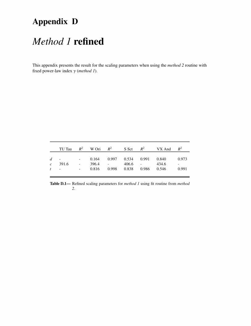
Appendix D

Method 1 refined

This appendix presents the result for the scaling parameters when using the method 2 routine withfixed power-law index γ (method 1).

TU Tau R2 W Ori R2 S Sct R2 VX And R2

d - - 0.164 0.997 0.534 0.991 0.840 0.973c 391.6 - 396.4 - 406.6 - 434.6 -t - - 0.816 0.998 0.838 0.986 0.546 0.991

Table D.1— Refined scaling parameters for method 1 using fit routine from method2.

106 APPENDIX D. METHOD 1 REFINED

Figure D.1— Resulting residual band emission when using method 2 with a fixedpower-law index of γ = 1 and W Ori as selected comparison star .

107

Figure D.2— Resulting residual band emission when using method 2 with a fixedpower-law index of γ = 1 and S Sct as selected comparison star .

108 APPENDIX D. METHOD 1 REFINED

Figure D.3— Resulting residual band emission when using method 2 with a fixedpower-law index of γ = 1 and VX And as selected comparison star .

christiaan boersma - kapteyn astronomical institute ... · project supervisors: ... these aspects...

Documents