CircuiTikZversion 0.2.3

Massimo A. Redaelli

November 18, 2009

Contents1 Introduction 2

1.1 About . . . . . . . . . . . . . . . . . . . . . . . . . . . . . . . . . 21.2 Loading the package . . . . . . . . . . . . . . . . . . . . . . . . . 31.3 License . . . . . . . . . . . . . . . . . . . . . . . . . . . . . . . . . 31.4 Feedback . . . . . . . . . . . . . . . . . . . . . . . . . . . . . . . 31.5 Requirements . . . . . . . . . . . . . . . . . . . . . . . . . . . . . 31.6 Incompatible packages . . . . . . . . . . . . . . . . . . . . . . . . 31.7 Introduction to version 0.2.3 . . . . . . . . . . . . . . . . . . . . . 31.8 ConTEXt compatibility . . . . . . . . . . . . . . . . . . . . . . . . 4

2 Options 4

3 The components 63.1 Monopoles . . . . . . . . . . . . . . . . . . . . . . . . . . . . . . . 63.2 Bipoles . . . . . . . . . . . . . . . . . . . . . . . . . . . . . . . . . 6

3.2.1 Instruments . . . . . . . . . . . . . . . . . . . . . . . . . . 63.2.2 Basic resistive bipoles . . . . . . . . . . . . . . . . . . . . 63.2.3 Resistors and the like . . . . . . . . . . . . . . . . . . . . 73.2.4 Stationary sources . . . . . . . . . . . . . . . . . . . . . . 83.2.5 Diodes and such . . . . . . . . . . . . . . . . . . . . . . . 93.2.6 Basic dynamical bipoles . . . . . . . . . . . . . . . . . . . 113.2.7 Sinusoidal sources . . . . . . . . . . . . . . . . . . . . . . 123.2.8 Switch . . . . . . . . . . . . . . . . . . . . . . . . . . . . . 12

3.3 Tripoles . . . . . . . . . . . . . . . . . . . . . . . . . . . . . . . . 123.3.1 Controlled sources . . . . . . . . . . . . . . . . . . . . . . 123.3.2 Transistors . . . . . . . . . . . . . . . . . . . . . . . . . . 133.3.3 Other bipole-like tripoles . . . . . . . . . . . . . . . . . . 16

3.4 Double bipoles . . . . . . . . . . . . . . . . . . . . . . . . . . . . 163.5 Logic gates . . . . . . . . . . . . . . . . . . . . . . . . . . . . . . 173.6 Operational Amplifier . . . . . . . . . . . . . . . . . . . . . . . . 193.7 Support shapes . . . . . . . . . . . . . . . . . . . . . . . . . . . . 20

1

4 Usage 204.1 Labels . . . . . . . . . . . . . . . . . . . . . . . . . . . . . . . . . 214.2 Currents . . . . . . . . . . . . . . . . . . . . . . . . . . . . . . . . 214.3 Voltages . . . . . . . . . . . . . . . . . . . . . . . . . . . . . . . . 22

4.3.1 European style . . . . . . . . . . . . . . . . . . . . . . . . 224.3.2 American style . . . . . . . . . . . . . . . . . . . . . . . . 22

4.4 Nodes . . . . . . . . . . . . . . . . . . . . . . . . . . . . . . . . . 234.5 Special components . . . . . . . . . . . . . . . . . . . . . . . . . . 234.6 Integration with siunitx . . . . . . . . . . . . . . . . . . . . . . 254.7 Mirroring . . . . . . . . . . . . . . . . . . . . . . . . . . . . . . . 264.8 Putting them together . . . . . . . . . . . . . . . . . . . . . . . . 26

5 Not only bipoles 275.1 Anchors . . . . . . . . . . . . . . . . . . . . . . . . . . . . . . . . 27

5.1.1 Logical ports . . . . . . . . . . . . . . . . . . . . . . . . . 275.1.2 Transistors . . . . . . . . . . . . . . . . . . . . . . . . . . 275.1.3 Other tripoles . . . . . . . . . . . . . . . . . . . . . . . . . 295.1.4 Operational amplifier . . . . . . . . . . . . . . . . . . . . 295.1.5 Double bipoles . . . . . . . . . . . . . . . . . . . . . . . . 30

5.2 Transistor paths . . . . . . . . . . . . . . . . . . . . . . . . . . . 30

6 Customization 316.1 Parameters . . . . . . . . . . . . . . . . . . . . . . . . . . . . . . 316.2 Components size . . . . . . . . . . . . . . . . . . . . . . . . . . . 326.3 Colors . . . . . . . . . . . . . . . . . . . . . . . . . . . . . . . . . 33

7 Examples 35

8 Revision history 37

1 IntroductionAfter two years of little exposure only on my personal website1, I did a majorrehauling of the code of CircuiTikZ, fixing several problems and convertingeverything to TikZ version 2.0.

I’m not too sure about the result, because my (La)TEX skills are much tobe improved, but it seems it’s time for more user feedback. So, here it is…

I know the documentation is somewhat scant. Hope to have time to improveit a bit.

1.1 AboutThis package provides a set of macros for naturally typesetting electrical and(somewhat less naturally, perhaps) electronical networks.

It was born mainly for writing my own exercise book and exams sheets forthe Elettrotecnica courses at Politecnico di Milano, Italy. I wanted a tool thatwas easy to use, with a lean syntax, native to LATEX, and supporting directlyPDF output format.

1http://home.dei.polimi.it/mredaelli.

2

So I based everything with the very impressive (if somewhat verbose attimes) TikZ package.

1.2 Loading the package\usepackagecircuitikz

TikZ will be automatically loaded.

1.3 LicenseCopyright © 2007–2009 Massimo Redaelli. This package is author-maintained.Permission is granted to copy, distribute and/or modify this software under theterms of the LATEXProject Public License, version 1.3.1, or the GNU PublicLicense. This software is provided ‘as is’, without warranty of any kind, eitherexpressed or implied, including, but not limited to, the implied warranties ofmerchantability and fitness for a particular purpose.

1.4 FeedbackMuch appreciated: mredaelli@elet.polimi.it. Although I don’t guaranteequick answers.

1.5 Requirements• tikz, version ≥ 2;

• xstring, not older than 2009/03/13;

• siunitx, if using siunitx option.

1.6 Incompatible packagesNone, as far as I know.

1.7 Introduction to version 0.2.3Having waited a long time before updating the package, many feature requestspiled on my desk. They should all be implemented now.

There are a number of backward incompatibilities—I’m sorry, but I had tomake a choice in order not to have a schizophrenic interface. They are mostly,in my opinion, minor problems that can be dealt with with appropriate packageoptions:

• potentiometer is now the standard resistor-with-arrow-in-the-middle; theold potentiometer is now known as variable resistor (or vR), similarlyto variable inductor and variable capacitor;

• american inductor was not really the standard american inductor. Theold american inductor has been renamed cute inductor;

• transformer, transformer core and variable inductor are now linkedwith the chosen type of inductor;

3

• styles for selecting shape variants (like [american resistors]) are nowin the plural to avoid conflict with paths (like to[american resistor]).

1.8 ConTEXt compatibilityAs requested by some users, I fixed the package for it to be compatible withConTEXt. Just use \usemodule[circuitikz] in your preamble and includethe code between \startcircuitikz and \endcircuitikz. Please notice thatthe package siunitx in not available for ConTEXt: the option siunitx simplydefines a few measurement units typical in electric sciences.

In actually using CircuiTikZ with TikZ version 2 in ConTEXt an error comesup, saying something like

! Undefined control sequence.\tikz@cc@mid@checks -> \pgfutil@ifnextchar!

The solution has been suggested to me by Aditya Mahajan, and involvesmodifying a file in TikZ:

Here is the fix. In tikzlibrarycalc.code.tex change

\def\tikz@cc@mid@checks\pgfutil@ifnextchar !%AM: Added space\tikz@cc@mid%

%\advance\pgf@xa by\tikz@cc@factor\pgf@xb%\advance\pgf@ya by\tikz@cc@factor\pgf@yb%\tikz@cc@parse% continue

%

\def\tikz@cc@mid !%AM Added space\pgfutil@ifnextchar(%\tikz@scan@one@point\tikz@cc@project%

%\tikz@cc@mid@num%

%

As far as I know, this is a bug in TikZ, and I notified the author, but untilhe fixes it, you know the workaround.

2 Options• europeanvoltages: uses arrows to define voltages, and uses european-

style voltage sources;

• americanvoltages: uses − and + to define voltages, and uses american-style voltage sources;

• europeancurrents: uses european-style current sources;

4

• americancurrents: uses american-style current sources;

• europeanresistors: uses rectangular empty shape for resistors, as pereuropean standards;

• americanresistors: uses zig-zag shape for resistors, as per americanstandards;

• europeaninductors: uses rectangular filled shape for inductors, as pereuropean standards;

• americaninductors: uses ”4-bumps” shape for inductors, as per americanstandards;

• cuteinductors: uses my personal favorite, ”pig-tailed” shape for induc-tors;

• americanports: uses triangular logic ports, as per american standards;

• europeanports: uses rectangular logic ports, as per european standards;

• european: equivalent to europeancurrents, europeanvoltages, europeanresistors,europeaninductors, europeanports;

• american: equivalent to americancurrents, americanvoltages, americanresistors,americaninductors, americanports;

• siunitx: integrates with SIunitx package. If labels, currents or voltagesare of the form #1<#2> then what is shown is actually \SI#1#2;

• nosiunitx: labels are not interpreted as above;

• fulldiodes: the various diodes are drawn and filled by default, i.e. whenusing styles such as diode, D, sD, …Un-filled diode can always be forcedwith Do, sDo, …

• emptydiodes: the various diodes are drawn but not filled by default, i.e.when using styles such as diode, D, sD, …Filled diode can always be forcedwith D*, sD*, …

• arrowmos: pmos and nmos have arrows analogous to those of pnp andnpn transistors;

• noarrowmos: pmos and nmos do not have arrows analogous to those ofpnp and npn transistors.

The old options in the singular (like american voltage) are still availablefor compatibility, but are discouraged.

Loading the package with no options is equivalent to my own personal liking,that is to the following options:[europeancurrents, europeanvoltages, americanresistors, cuteinductors,americanports, nosiunitx, noarrowmos].

In ConTEXt the options are similarly specified: current=european|american,voltage=european|american, resistor=american|european, inductor=cute|american|european,logic=american|european, siunitx=true|false, arrowmos=false|true.

5

3 The componentsHere follows the list of all the shapes defined by CircuiTikZ. These are all pgfnodes, so they are usable in both pgf and TikZ.

Each bipole (plus triac and thyristors) are shown using the following com-mand, where #1 is the name of the component2:

\begincenter\begincircuitikz \draw(0,0) to[ #1 ] (2,0)

; \endcircuitikz \endcenter

The other shapes are shown with:

\begincenter\begincircuitikz \draw(0,0) node[ #1 ]

; \endcircuitikz \endcenter

Please notice that for user convenience transistors can also be inputted usingthe syntax for bipoles. See section 5.2.

3.1 Monopoles• Ground (ground)

..

3.2 Bipoles3.2.1 Instruments

• Ammeter (ammeter)

. .A.

.

• Voltmeter (voltmeter)

. .V.

.

3.2.2 Basic resistive bipoles

• Short circuit (short)

. .

• Open circuit (open)2If #1 is the name of the bipole/the style, then the actual name of the shape is #1shape.

6

. .

• Lamp (lamp)

. .

• Generic (symmetric) bipole (generic)

. .

• Tunable generic bipole (tgeneric)

. .

• Generic asymmetric bipole (ageneric)

. .

• Generic asymmetric bipole (full) (fullgeneric)

. .

• Tunable generic bipole (full) (tfullgeneric)

. .

• Memristor (memristor, or Mr)

. .

3.2.3 Resistors and the like

If (default behaviour) americanresistors option is active (or the style [americanresistors] is used), the resistor is displayed as follows:

• Resistor (R, or american resistor)

. .

• Variable resistor (vR, or american variable resistor)

. .

7

• Potentiometer (pR, or american potentiometer)

. .

If instead europeanresistors option is active (or the style [europeanresistors] is used), the resistors, variable resistors and potentiometers aredisplayed as follows:

• Resistor (R, or european resistor)

. .

• Variable resistor (vR, or european variable resistor)

. .

• Potentiometer (pR, or european potentiometer)

. .

3.2.4 Stationary sources

• Battery (battery)

. .

• Voltage source (european style) (european voltage source)

. .

• Voltage source (american style) (american voltage source)

. .+.− .

• Current source (european style) (european current source)

. .

• Current source (american style) (american current source)

. ..

8

If (default behaviour) europeancurrents option is active (or the style[european currents] is used), the shorthands current source, isource,and I are equivalent to european current source. Otherwise, ifamericancurrents option is active (or the style [american currents]is used) they are equivalent to american current source.

Similarly, if (default behaviour) europeanvoltages option is active (orthe style [european voltages] is used), the shorthands voltage source,vsource, and V are equivalent to european voltage source. Otherwise,if americanvoltages option is active (or the style [american voltages]is used) they are equivalent to american voltage source.

3.2.5 Diodes and such

• Empty diode (empty diode, or Do)

. .

• Empty Schottky diode (empty Schottky diode, or sDo)

. .

• Empty Zener diode (empty Zener diode, or zDo)

. .

• Empty tunnel diode (empty tunnel diode, or tDo)

. .

• Empty photodiode (empty photodiode, or pDo)

. .

• Empty led (empty led, or leDo)

. .

• Empty varcap (empty varcap, or VCo)

. .

9

• Full diode (full diode, or D*)

. .

• Full Schottky diode (full Schottky diode, or sD*)

. .

• Full Zener diode (full Zener diode, or zD*)

. .

• Full tunnel diode (full tunnel diode, or tD*)

. .

• Full photodiode (full photodiode, or pD*)

. .

• Full led (full led, or leD*)

. .

• Full varcap (full varcap, or VC*)

. .

The options fulldiodes and emptydiodes (and the styles [fulldiodes] and [empty diodes]) define which shape will be used by ab-breviated commands such that D, sD, zD, tD, pD, leD, and VC.

10

3.2.6 Basic dynamical bipoles

• Capacitor (capacitor, or C)

. .

• Polar capacitor (polar capacitor, or pC)

. .

• Variable capacitor (variable capacitor, or vC)

. .

If (default behaviour) cuteinductors option is active (or the style [cuteinductors] is used), the inductors are displayed as follows:

• Inductor (L, or cute inductor)

. .

• Variable inductor (vL, or variable cute inductor)

. .

If americaninductors option is active (or the style [american inductors]is used), the inductors are displayed as follows:

• Inductor (L, or american inductor)

. .

• Variable inductor (vL, or variable american inductor)

. .

Finally, if europeaninductors option is active (or the style [europeaninductors] is used), the inductors are displayed as follows:

• Inductor (L, or european inductor)

. .

• Variable inductor (vL, or variable european inductor)

. .

11

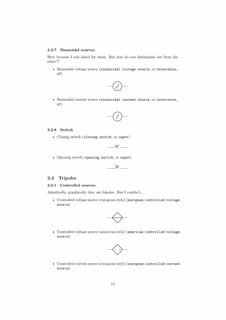
3.2.7 Sinusoidal sources

Here because I was asked for them. But how do you distinguish one from theother?!

• Sinusoidal voltage source (sinusoidal voltage source, or vsourcesin,sV)

. .

• Sinusoidal current source (sinusoidal current source, or isourcesin,sI)

. .

3.2.8 Switch

• Closing switch (closing switch, or cspst)

. .

• Opening switch (opening switch, or ospst)

. .

3.3 Tripoles3.3.1 Controlled sources

Admittedly, graphically they are bipoles. But I couldn’t…

• Controlled voltage source (european style) (european controlled voltagesource)

. .

• Controlled voltage source (american style) (american controlled voltagesource)

. .+.− .

• Controlled current source (european style) (european controlled currentsource)

12

. .

• Controlled current source (american style) (american controlled currentsource)

. ..

If (default behaviour) europeancurrents option is active (or the style[european currents] is used), the shorthands controlled currentsource, cisource, and cI are equivalent to european controlledcurrent source. Otherwise, if americancurrents option is active (orthe style [american currents] is used) they are equivalent to americancontrolled current source.

Similarly, if (default behaviour) europeanvoltages option is ac-tive (or the style [european voltages] is used), the shorthandscontrolled voltage source, cvsource, and cV are equivalent toeuropean controlled voltage source. Otherwise, if americanvoltagesoption is active (or the style [american voltages] is used) they are equiv-alent to american controlled voltage source.

• Controlled sinusoidal voltage source (controlled sinusoidal voltagesource, or controlled vsourcesin, cvsourcesin, csV)

. .

• Controlled sinusoidal current source (controlled sinusoidal currentsource, or controlled isourcesin, cisourcesin, csI)

. .

3.3.2 Transistors

• nmos (nmos)

..

• pmos (pmos)

13

..

• npn (npn)

..

.

• pnp (pnp)

.. .

• npigbt (nigbt)

..

.

• pigbt (pigbt)

.. .

If the option arrowmos is used (or after the commant \ctikzsettripoles/mos style/arrowsis given), this is the output:

• nmos (nmos)

..

.

• pmos (pmos)

.

. .

14

nfets and pfets have been incorporated based on code provided by ClemensHelfmeier and Theodor Borsche:

• nfet (nfet)

..

.

• nigfete (nigfete)

..

.

• nigfetd (nigfetd)

..

.

• pfet (pfet)

...

• pigfete (pigfete)

...

• pigfetd (pigfetd)

...

njfet and pjfet have been incorporated based on code provided by DaniloPiazzalunga:

• njfet (njfet)

15

..

.

• pjfet (pjfet)

.

. .

3.3.3 Other bipole-like tripoles

The following tripoles are entered with the usual command of the form

• triac (triac, or Tr)

. .

• thyristor (thyristor, or Ty)

. .

3.4 Double bipolesTransformers automatically use the inductor shape currently selected. Theseare the three possibilities:

• Transformer (cute inductor) (transformer).

. ..

• Transformer (american inductor) (transformer).

. ..

16

• Transformer (european inductor) (transformer).

. ..

Transformers with core are also available:

• Transformer core (cute inductor) (transformer core).

. ..

• Transformer core (american inductor) (transformer core).

. ..

• Transformer core (european inductor) (transformer core).

. ..

• Gyrator (gyrator).

.

3.5 Logic gates• American and port (american and port)

..

17

• American or port (american or port)

..

• American not port (american not port)

..

• American nand port (american nand port)

..

• American nor port (american nor port)

..

• American xor port (american xor port)

..

• American xnor port (american xnor port)

..

• European and port (european and port)

..&.

• European or port (european or port)

..≥ 1.

• European not port (european not port)

18

..1.

• European nand port (european nand port)

..&.

• European nor port (european nor port)

..≥ 1.

• European xor port (european xor port)

..= 1.

• European xnor port (european xnor port)

..= 1.

If (default behaviour) americanports option is active (or the style[american ports] is used), the shorthands and port, or port, not port,nand port, not port, xor port, and xnor port are equivalent to theamerican version of the respective logic port.

If otherwise europeanports option is active (or the style [europeanports] is used), the shorthands and port, or port, not port, nand port,not port, xor port, and xnor port are equivalent to the european versionof the respective logic port.

3.6 Operational Amplifier• Operational amplifier (op amp)

..−

.+.

19

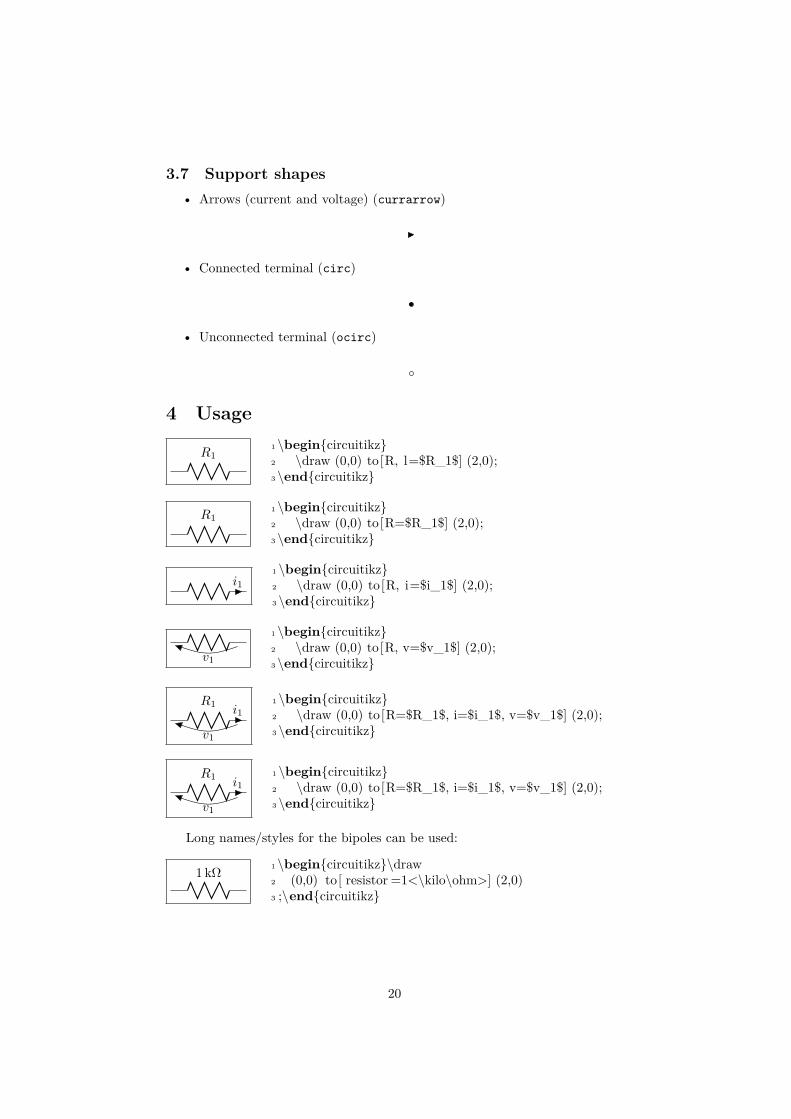
3.7 Support shapes• Arrows (current and voltage) (currarrow)

..

• Connected terminal (circ)

..

• Unconnected terminal (ocirc)

..

4 Usage

. ..R1

1 \begincircuitikz2 \draw (0,0) to[R, l=$R_1$] (2,0);3 \endcircuitikz

. ..R1

1 \begincircuitikz2 \draw (0,0) to[R=$R_1$] (2,0);3 \endcircuitikz

. . ..i11 \begincircuitikz2 \draw (0,0) to[R, i=$i_1$] (2,0);3 \endcircuitikz

. ..

.v1

1 \begincircuitikz2 \draw (0,0) to[R, v=$v_1$] (2,0);3 \endcircuitikz

. ..R1

.

.v1

..i11 \begincircuitikz2 \draw (0,0) to[R=$R_1$, i=$i_1$, v=$v_1$] (2,0);3 \endcircuitikz

. ..R1

.

.v1

..i11 \begincircuitikz2 \draw (0,0) to[R=$R_1$, i=$i_1$, v=$v_1$] (2,0);3 \endcircuitikz

Long names/styles for the bipoles can be used:

. ..1 kΩ

1 \begincircuitikz\draw2 (0,0) to[ resistor =1<\kilo\ohm>] (2,0)3 ;\endcircuitikz

20

4.1 Labels

. ..R1

1 \begincircuitikz2 \draw (0,0) to[R, l^=$R_1$] (2,0);3 \endcircuitikz

. ..R1

1 \begincircuitikz2 \draw (0,0) to[R, l_=$R_1$] (2,0);3 \endcircuitikz

4.2 Currents

. . ..i11 \begincircuitikz2 \draw (0,0) to[R, i^>=$i_1$] (2,0);3 \endcircuitikz

. . ..i1

1 \begincircuitikz2 \draw (0,0) to[R, i_>=$i_1$] (2,0);3 \endcircuitikz

. . ..i11 \begincircuitikz2 \draw (0,0) to[R, i^<=$i_1$] (2,0);3 \endcircuitikz

. . ..i1

1 \begincircuitikz2 \draw (0,0) to[R, i_<=$i_1$] (2,0);3 \endcircuitikz

. ...i11 \begincircuitikz2 \draw (0,0) to[R, i>^=$i_1$] (2,0);3 \endcircuitikz

. ...i1

1 \begincircuitikz2 \draw (0,0) to[R, i>_=$i_1$] (2,0);3 \endcircuitikz

. ...i11 \begincircuitikz2 \draw (0,0) to[R, i<^=$i_1$] (2,0);3 \endcircuitikz

. ..

.i11 \begincircuitikz2 \draw (0,0) to[R, i<_=$i_1$] (2,0);3 \endcircuitikz

Also

. . ..i11 \begincircuitikz2 \draw (0,0) to[R, i<=$i_1$] (2,0);3 \endcircuitikz

. . ..i11 \begincircuitikz2 \draw (0,0) to[R, i>=$i_1$] (2,0);3 \endcircuitikz

21

. . ..i11 \begincircuitikz2 \draw (0,0) to[R, i^=$i_1$] (2,0);3 \endcircuitikz

. . ..i1

1 \begincircuitikz2 \draw (0,0) to[R, i_=$i_1$] (2,0);3 \endcircuitikz

4.3 Voltages4.3.1 European style

The default, with arrows. Use option europeanvoltage or style [european voltages].

. . ..v1

1 \begincircuitikz[european voltages]2 \draw (0,0) to[R, v^>=$v_1$] (2,0);3 \endcircuitikz

. ..

.v11 \begincircuitikz[european voltages]2 \draw (0,0) to[R, v^<=$v_1$] (2,0);3 \endcircuitikz

. . ..v1

1 \begincircuitikz[european voltages]2 \draw (0,0) to[R, v_>=$v_1$] (2,0);3 \endcircuitikz

. ..

.v1

1 \begincircuitikz[european voltages]2 \draw (0,0) to[R, v_<=$v_1$] (2,0);3 \endcircuitikz

4.3.2 American style

For those who like it (not me). Use option americanvoltage or set [american voltages].

. ..− .+.v11 \begincircuitikz[american voltages]2 \draw (0,0) to[R, v^>=$v_1$] (2,0);3 \endcircuitikz

. ..+ .−.v11 \begincircuitikz[american voltages]2 \draw (0,0) to[R, v^<=$v_1$] (2,0);3 \endcircuitikz

. ..− .+.v1

1 \begincircuitikz[american voltages]2 \draw (0,0) to[R, v_>=$v_1$] (2,0);3 \endcircuitikz

. ..+ .−.v1

1 \begincircuitikz[american voltages]2 \draw (0,0) to[R, v_<=$v_1$] (2,0);3 \endcircuitikz

22

4.4 Nodes

. .. .1 \begincircuitikz2 \draw (0,0) to[R, o−o] (2,0);3 \endcircuitikz

. . .1 \begincircuitikz2 \draw (0,0) to[R, −o] (2,0);3 \endcircuitikz

. ..1 \begincircuitikz2 \draw (0,0) to[R, o−] (2,0);3 \endcircuitikz

. .. .1 \begincircuitikz2 \draw (0,0) to[R, *−*] (2,0);3 \endcircuitikz

. . .1 \begincircuitikz2 \draw (0,0) to[R, −*] (2,0);3 \endcircuitikz

. ..1 \begincircuitikz2 \draw (0,0) to[R, *−] (2,0);3 \endcircuitikz

. .. .1 \begincircuitikz2 \draw (0,0) to[R, o−*] (2,0);3 \endcircuitikz

. .. .1 \begincircuitikz2 \draw (0,0) to[R, *−o] (2,0);3 \endcircuitikz

4.5 Special componentsFor some components label, current and voltage behave as one would expect:

. . .

.a1 1 \begincircuitikz2 \draw (0,0) to[ I=$a_1$] (2,0);3 \endcircuitikz

. . .

.a1 1 \begincircuitikz2 \draw (0,0) to[ I , i=$a_1$] (2,0);3 \endcircuitikz

. . .

.k · a1 1 \begincircuitikz2 \draw (0,0) to[ cI=$k\cdot a_1$] (2,0);3 \endcircuitikz

23

. . .

.a1 1 \begincircuitikz2 \draw (0,0) to[ sI=$a_1$] (2,0);3 \endcircuitikz

. . .

.k · a1 1 \begincircuitikz2 \draw (0,0) to[ csI=$k\cdot a_1$] (2,0);3 \endcircuitikz

The following results from using the option americancurrent or using thestyle [american currents].

. ..

.a1 1 \begincircuitikz[american currents]2 \draw (0,0) to[ I=$a_1$] (2,0);3 \endcircuitikz

. ..

.a1 1 \begincircuitikz[american currents]2 \draw (0,0) to[ I , i=$a_1$] (2,0);3 \endcircuitikz

. ..

.k · a1 1 \begincircuitikz[american currents]2 \draw (0,0) to[ cI=$k\cdot a_1$] (2,0);3 \endcircuitikz

. .

.a1 1 \begincircuitikz[american currents]2 \draw (0,0) to[ sI=$a_1$] (2,0);3 \endcircuitikz

. .

.k · a1 1 \begincircuitikz[american currents]2 \draw (0,0) to[ csI=$k\cdot a_1$] (2,0);3 \endcircuitikz

The same holds for voltage sources:

. ...a1 1 \begincircuitikz

2 \draw (0,0) to[V=$a_1$] (2,0);3 \endcircuitikz

. ...a1 1 \begincircuitikz

2 \draw (0,0) to[V, v=$a_1$] (2,0);3 \endcircuitikz

. .

..k · a11 \begincircuitikz2 \draw (0,0) to[cV=$k\cdot a_1$] (2,0);3 \endcircuitikz

24

. ...a1 1 \begincircuitikz

2 \draw (0,0) to[sV=$a_1$] (2,0);3 \endcircuitikz

. .

..k · a11 \begincircuitikz2 \draw (0,0) to[csV=$k\cdot a_1$] (2,0);3 \endcircuitikz

The following results from using the option americanvoltage or the style[american voltages].

. .+.− ..a1 1 \begincircuitikz[american voltages]

2 \draw (0,0) to[V=$a_1$] (2,0);3 \endcircuitikz

. .+.− ..a1 1 \begincircuitikz[american voltages]

2 \draw (0,0) to[V, v=$a_1$] (2,0);3 \endcircuitikz

. .+.− .

.k · a1 1 \begincircuitikz[american voltages]2 \draw (0,0) to[cV=$k\cdot a_1$] (2,0);3 \endcircuitikz

. ..a1 1 \begincircuitikz[american voltages]

2 \draw (0,0) to[sV=$a_1$] (2,0);3 \endcircuitikz

. .

.k · a1 1 \begincircuitikz[american voltages]2 \draw (0,0) to[csV=$k\cdot a_1$] (2,0);3 \endcircuitikz

4.6 Integration with siunitxIf the option siunitx is active (and not in ConTEXt), then the following areequivalent:

. ..1 kΩ

1 \begincircuitikz2 \draw (0,0) to[R, l=1<\kilo\ohm>] (2,0);3 \endcircuitikz

. ..1 kΩ

1 \begincircuitikz2 \draw (0,0) to[R, l=$\SI1\kilo\ohm$] (2,0);3 \endcircuitikz

. . ..1 mA1 \begincircuitikz2 \draw (0,0) to[R, i=1<\milli\ampere>] (2,0);3 \endcircuitikz

25

. . ..1 mA1 \begincircuitikz2 \draw (0,0) to[R, i=$\SI1\milli\ampere$] (2,0);3 \endcircuitikz

. ..

.1 V

1 \begincircuitikz2 \draw (0,0) to[R, v=1<\volt>] (2,0);3 \endcircuitikz

. ..

.1 V

1 \begincircuitikz2 \draw (0,0) to[R, v=$\SI1\volt$] (2,0);3 \endcircuitikz

4.7 Mirroring

. .1 \begincircuitikz2 \draw (0,0) to[pD] (2,0);3 \endcircuitikz

. .1 \begincircuitikz2 \draw (0,0) to[pD, mirror] (2,0);3 \endcircuitikz

At the moment, placing labels and currents on mirrored bipoles works:

. ..T

1 \begincircuitikz2 \draw (0,0) to[ospst=T] (2,0);3 \endcircuitikz

. .

.T

..i1 1 \begincircuitikz2 \draw (0,0) to[ospst=T, mirror, i=$i_1$] (2,0);3 \endcircuitikz

But voltages don’t:

. .

.T

. .v 1 \begincircuitikz2 \draw (0,0) to[ospst=T, mirror, v=v] (2,0);3 \endcircuitikz

Sorry about that.

4.8 Putting them together

. ..1 kΩ

. ...1 mA

1 \begincircuitikz2 \draw (0,0) to[R=1<\kilo\ohm>,3 i>_=1<\milli\ampere>, o−*] (3,0);4 \endcircuitikz

. .. ..

.vD

..1 mA1 \begincircuitikz2 \draw (0,0) to[D*, v=$v_D$,3 i=1<\milli\ampere>, o−*] (3,0);4 \endcircuitikz

26

5 Not only bipolesSince only bipoles (but see section 5.2) can be placed ”along a line”, componentswith more than two terminals are placed as nodes:

..

.1 \tikz \node[npn] at (0,0) ;

5.1 AnchorsIn order to allow connections with other components, all components defineanchors.

5.1.1 Logical ports

All logical ports, except not, have to inputs and one output. They are calledrespectively in 1, in 2, out:

...1.2

.3

1 \begincircuitikz \draw2 (0,0) node[and port] (myand) 3 (myand.in 1) node[anchor=east] 14 (myand.in 2) node[anchor=east] 25 (myand.out) node[anchor=west] 36 ;\endcircuitikz

.

.

.

.

1 \begincircuitikz \draw2 (0,2) node[and port] (myand1) 3 (0,0) node[and port] (myand2) 4 (2,1) node[xnor port] (myxnor) 5 (myand1.out) −| (myxnor.in 1)6 (myand2.out) −| (myxnor.in 2)7 ;\endcircuitikz

In the case of not, there are only in and out (although for compatibilityreasons in 1 is still defined and equal to in):

. . .

.

.

1 \begincircuitikz \draw2 (1,0) node[not port] (not1) 3 (3,0) node[not port] (not2) 4 (0,0) −− (not1.in)5 (not2.in) −− (not1.out)6 ++(0,−1) node[ground] to[C] (not1.out)7 (not2.out) −| (4,1) −| (0,0)8 ;\endcircuitikz

5.1.2 Transistors

For nmos, pmos, nfet, nigfete, nigfetd, pfet, pigfete, and pigfetd tran-sistors one has base, gate, source and drain anchors (which can be abbreviatedwith B, G, S and D):

27

..

.B.G

.D

.S

1 \begincircuitikz \draw2 (0,0) node[nmos] (mos) 3 (mos.base) node[anchor=west] B4 (mos.gate) node[anchor=east] G5 (mos.drain) node[anchor=south] D6 (mos.source) node[anchor=north] S7 ;\endcircuitikz

....B

.G

.D

.S

1 \begincircuitikz \draw2 (0,0) node[pigfete ] ( pigfete ) 3 ( pigfete .B) node[anchor=west] B4 ( pigfete .G) node[anchor=east] G5 ( pigfete .D) node[anchor=south] D6 ( pigfete .S) node[anchor=north] S7 ;\endcircuitikz

Similarly njfet and pjfet have gate, source and drain anchors (whichcan be abbreviated with G, S and D):

.

. ..G

.D

.S 1 \begincircuitikz \draw2 (0,0) node[pjfet ] ( pjfet ) 3 (pjfet .G) node[anchor=east] G4 (pjfet .D) node[anchor=north] D5 (pjfet .S) node[anchor=south] S6 ;\endcircuitikz

For npn, pnp, nigbt, and pigbt transistors the anchors are base, emitterand collector anchors (which can be abbreviated with B, E and C):

..

..B

.C

.E

1 \begincircuitikz \draw2 (0,0) node[npn] (npn) 3 (npn.base) node[anchor=east] B4 (npn.collector ) node[anchor=south] C5 (npn.emitter) node[anchor=north] E6 ;\endcircuitikz

.. ..B

.C

.E 1 \begincircuitikz \draw2 (0,0) node[pigbt] (pigbt) 3 (pigbt.B) node[anchor=east] B4 (pigbt.C) node[anchor=north] C5 (pigbt.E) node[anchor=south] E6 ;\endcircuitikz

Here is one composite example (please notice that the xscale=-1 style wouldalso reflect the label of the transistors, so here a new node is added and its textis used, instead of that of pnp1):

28

.. .2...1

.

.

.

.

.

.

1 \begincircuitikz \draw2 (0,0) node[pnp] (pnp2) 23 (pnp2.B) node[pnp, xscale=−1, anchor=B] (pnp1) 4 (pnp1) node 15 (pnp1.C) node[npn, anchor=C] (npn1) 6 (pnp2.C) node[npn, xscale=−1, anchor=C] (npn2) 7 (pnp1.E) −− (pnp2.E) (npn1.E) −− (npn2.E)8 (pnp1.B) node[circ] |− (pnp2.C) node[circ] 9 ;\endcircuitikz

Similarly, transistors can be reflected vertically:

....B

.G

.D

.S1 \begincircuitikz \draw2 (0,0) node[pigfete , yscale=−1] (pigfete) 3 ( pigfete .B) node[anchor=west] B4 ( pigfete .G) node[anchor=east] G5 ( pigfete .D) node[anchor=north] D6 ( pigfete .S) node[anchor=south] S7 ;\endcircuitikz

5.1.3 Other tripoles

When inserting a thrystor, a triac or a potentiometer, one needs to refer to thethird node—gate (gate or G) for the former two; wiper (wiper or W) for thelatter one. This is done by giving a name to the bipole:

. . .

1 \begincircuitikz \draw2 (0,0) to[Tr, n=TRI] (2,0)3 to[pR, n=POT] (4,0);4 \draw[dashed] (TRI.G) −| (POT.wiper)5 ;\endcircuitikz

5.1.4 Operational amplifier

The op amp defines the inverting input (-), the non-inverting input (+) and theoutput (out) anchors:

..−

.+.

.v+

.v−.vo

1 \begincircuitikz \draw2 (0,0) node[op amp] (opamp) 3 (opamp.+) node[left] $v_+$4 (opamp.−) node[left] $v_−$5 (opamp.out) node[right] $v_o$6 ;\endcircuitikz

There are also two more anchors defined, up and down, for the power supplies:

29

..−

.+.

.v+

.v−.vo

.

.12 V

1 \begincircuitikz \draw2 (0,0) node[op amp] (opamp) 3 (opamp.+) node[left] $v_+$4 (opamp.−) node[left] $v_−$5 (opamp.out) node[right] $v_o$6 (opamp.down) node[ground] 7 (opamp.up) ++ (0,.5) node[above] \SI12\volt8 −− (opamp.up)9 ;\endcircuitikz

5.1.5 Double bipoles

All the (few, actually) double bipoles/quadrupoles have the four anchors, twofor each port. The first port, to the left, is port A, having the anchors A1 (up)and A2 (down); same for port B. They also expose the base anchor, for labelling:

.

. ..

.A1

.A2

.B1

.B2

.K1 \begincircuitikz \draw2 (0,0) node[transformer] (T) 3 (T.A1) node[anchor=east] A14 (T.A2) node[anchor=east] A25 (T.B1) node[anchor=west] B16 (T.B2) node[anchor=west] B27 (T.base) nodeK8 ;\endcircuitikz

.

.

.A1

.A2

.B1

.B2

.K1 \begincircuitikz \draw2 (0,0) node[gyrator] (G) 3 (G.A1) node[anchor=east] A14 (G.A2) node[anchor=east] A25 (G.B1) node[anchor=west] B16 (G.B2) node[anchor=west] B27 (G.base) nodeK8 ;\endcircuitikz

5.2 Transistor pathsFor syntactical convenience transistors can be placed using the normal pathnotation used for bipoles. The transitor type can be specified by simply addinga “T” (for transistor) in front of the node name of the transistor. It will beplaced with the base/gate orthogonal to the direction of the path:

..

.1

.

..2.

..3 1 \begincircuitikz \draw2 (0,0) node[njfet ] 13 (−1,2) to[Tnjfet=2] (1,2)4 to[Tnjfet=3, mirror] (3,2);5 ;\endcircuitikz

30

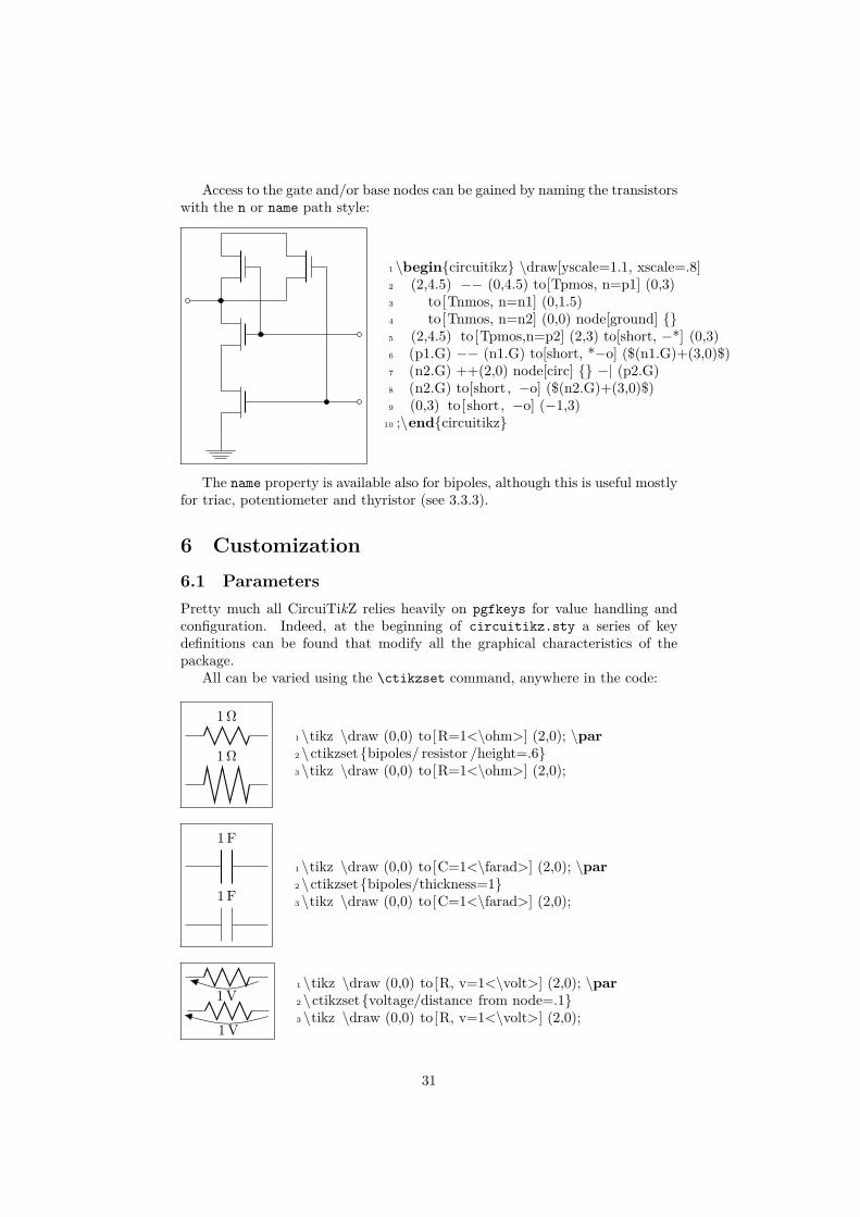
Access to the gate and/or base nodes can be gained by naming the transistorswith the n or name path style:

.

.

.

.

.

.

.

.

.

.

..

.. .

.. .

..

1 \begincircuitikz \draw[yscale=1.1, xscale=.8]2 (2,4.5) −− (0,4.5) to[Tpmos, n=p1] (0,3)3 to[Tnmos, n=n1] (0,1.5)4 to[Tnmos, n=n2] (0,0) node[ground] 5 (2,4.5) to[Tpmos,n=p2] (2,3) to[short, −*] (0,3)6 (p1.G) −− (n1.G) to[short, *−o] ($(n1.G)+(3,0)$)7 (n2.G) ++(2,0) node[circ] −| (p2.G)8 (n2.G) to[short, −o] ($(n2.G)+(3,0)$)9 (0,3) to[short, −o] (−1,3)

10 ;\endcircuitikz

The name property is available also for bipoles, although this is useful mostlyfor triac, potentiometer and thyristor (see 3.3.3).

6 Customization6.1 ParametersPretty much all CircuiTikZ relies heavily on pgfkeys for value handling andconfiguration. Indeed, at the beginning of circuitikz.sty a series of keydefinitions can be found that modify all the graphical characteristics of thepackage.

All can be varied using the \ctikzset command, anywhere in the code:

. ..1 Ω

. ..1 Ω

1 \tikz \draw (0,0) to[R=1<\ohm>] (2,0); \par2 \ctikzsetbipoles/ resistor /height=.63 \tikz \draw (0,0) to[R=1<\ohm>] (2,0);

. ..1 F

. ..1 F

1 \tikz \draw (0,0) to[C=1<\farad>] (2,0); \par2 \ctikzsetbipoles/thickness=13 \tikz \draw (0,0) to[C=1<\farad>] (2,0);

. ..

.1 V. ..

.1 V

1 \tikz \draw (0,0) to[R, v=1<\volt>] (2,0); \par2 \ctikzsetvoltage/distance from node=.13 \tikz \draw (0,0) to[R, v=1<\volt>] (2,0);

31

..

..

1 \tikz \draw (0,0) node[nand port] ; \par2 \ctikzset tripoles /american nand port/input height=.23 \ctikzset tripoles /american nand port/port width=.24 \tikz \draw (0,0) node[nand port] ;

. . ..ı

. . ..ı

1 \tikz \draw (0,0) to[C, i=$\imath$] (2,0); \par2 \ctikzsetcurrent/distance = .23 \tikz \draw (0,0) to[C, i=$\imath$] (2,0);

Admittedly, not all graphical properties have understandable names, but forthe time it will have to do:

.. ..1 \tikz \draw (0,0) node[xnor port] ;2 \ctikzset tripoles /american xnor port/aaa=.23 \ctikzset tripoles /american xnor port/bbb=.64 \tikz \draw (0,0) node[xnor port] ;

6.2 Components sizePerhaps the most important parameter is \circuitikzbasekey/bipoles/length,which can be interpreted as the length of a resistor (including reasonable con-nections): all other lenghts are relative to this value. For instance:

..B .. .

..20 Ω

.

. ..10 Ω

.

.vx

.

.

.

.

.S5vx

..5 Ω

.

....A

1 \ctikzsetbipoles/length=1.4cm2 \begincircuitikz[scale=1.2]\draw3 (0,0) node[anchor=east] B4 to[short, o−*] (1,0)5 to[R=20<\ohm>, *−*] (1,2)6 to[R=10<\ohm>, v=$v_x$] (3,2) −− (4,2)7 to[ cI=$\frac\siemens5 v_x$, *−*] (4,0) −− (3,0)8 to[R=5<\ohm>, *−*] (3,2)9 (3,0) −− (1,0)

10 (1,2) to[short, −o] (0,2) node[anchor=east]A11 ;\endcircuitikz

32

..B .. .

..20 Ω

.

. ..10 Ω

.

.vx

.

.

.

.

.S5vx

..5 Ω

.

....A

1 \ctikzsetbipoles/length=.8cm2 \begincircuitikz[scale=1.2]\draw3 (0,0) node[anchor=east] B4 to[short, o−*] (1,0)5 to[R=20<\ohm>, *−*] (1,2)6 to[R=10<\ohm>, v=$v_x$] (3,2) −− (4,2)7 to[ cI=$\frac\siemens5 v_x$, *−*] (4,0) −− (3,0)8 to[R=5<\ohm>, *−*] (3,2)9 (3,0) −− (1,0)

10 (1,2) to[short, −o] (0,2) node[anchor=east]A11 ;\endcircuitikz

6.3 ColorsThe color of the components is stores in the key \circuitikzbasekey/color.CircuiTikZ tries to follow the color set in TikZ, although sometimes it fails. Ifyou change color in the picture, please do not use just the color name as a style,like [red], but rather assign the style [color=red].

Compare for instance

.

.

.

.

1 \begincircuitikz \draw[red]2 (0,2) node[and port] (myand1) 3 (0,0) node[and port] (myand2) 4 (2,1) node[xnor port] (myxnor) 5 (myand1.out) −| (myxnor.in 1)6 (myand2.out) −| (myxnor.in 2)7 ;\endcircuitikz

and

.

.

.

.

1 \begincircuitikz \draw[color=red]2 (0,2) node[and port] (myand1) 3 (0,0) node[and port] (myand2) 4 (2,1) node[xnor port] (myxnor) 5 (myand1.out) −| (myxnor.in 1)6 (myand2.out) −| (myxnor.in 2)7 ;\endcircuitikz

One can of course change the color in medias res:

33

.. ...

.

.

.

.

.

.

1 \begincircuitikz \draw2 (0,0) node[pnp, color=blue] (pnp2) 3 (pnp2.B) node[pnp, xscale=−1, anchor=B, color=brown] (pnp1) 4 (pnp1.C) node[npn, anchor=C, color=green] (npn1) 5 (pnp2.C) node[npn, xscale=−1, anchor=C, color=magenta] (npn2) 6 (pnp1.E) −− (pnp2.E) (npn1.E) −− (npn2.E)7 (pnp1.B) node[circ] |− (pnp2.C) node[circ] 8 ;\endcircuitikz

The all-in-one stream of bipoles poses some challanges, as only the actualbody of the bipole, and not the connecting lines, will be rendered in the specifiedcolor. Also, please notice the curly braces around the to:

.

..

.1 V

..1 Ω

. .1 F

1 \begincircuitikz \draw2 (0,0) to[V=1<\volt>] (0,2)3 to[R=1<\ohm>, color=red] (2,2) 4 to[C=1<\farad>] (2,0) −− (0,0)5 ;\endcircuitikz

Which, for some bipoles, can be frustrating:

.

..

.1 V

..1 Ω

. .1 F

1 \begincircuitikz \draw2 (0,0)to[V=1<\volt>, color=red] (0,2) 3 to[R=1<\ohm>] (2,2)4 to[C=1<\farad>] (2,0) −− (0,0)5 ;\endcircuitikz

The only way out is to specify different paths:

.

..

.1 V

..1 Ω

. .1 F

1 \begincircuitikz \draw[color=red]2 (0,0) to[V=1<\volt>, color=red] (0,2);3 \draw (0,2) to[R=1<\ohm>] (2,2)4 to[C=1<\farad>] (2,0) −− (0,0)5 ;\endcircuitikz

And yes: this is a bug and not a feature…

34

7 Examples

.

..10 µF

..2.2 kΩ

. .12 mH. .i1

.

.

.

..1 kΩ

. .

..0.3 kΩi1

.

.

..1 mA

1 \begincircuitikz[scale=1.4]\draw2 (0,0) to[C, l=10<\micro\farad>] (0,2) −− (0,3)3 to[R, l=2.2<\kilo\ohm>] (4,3) −− (4,2)4 to[L, l=12<\milli\henry>, i=$i_1$] (4,0) −− (0,0)5 (4,2) to[D*, *−*, color=red] (2,0) 6 (0,2) to[R, l=1<\kilo\ohm>, *−] (2,2)7 to[cV, v=$\SI.3\kilo\ohm i_1$] (4,2)8 (2,0) to[ I , i=1<\milli\ampere>, −*] (2,2)9 ;\endcircuitikz

..

.

.

.

.

.e(t)

..4 nF

..1/4 kΩ

.

.

..1 kΩ

..2 nF

.

.

.

.

.

.a(t)

..2 mH

.1 .2 .3

1 \begincircuitikz[scale=1.2]\draw2 (0,0) node[ground] 3 to[V=$e(t)$, *−*] (0,2) to[C=4<\nano\farad>] (2,2)4 to[R, l_=1/4<\kilo\ohm>, *−*] (2,0)5 (2,2) to[R=1<\kilo\ohm>] (4,2)6 to[C, l_=2<\nano\farad>, *−*] (4,0)7 (5,0) to[ I , i_=$a(t)$, −*] (5,2) −− (4,2)8 (0,0) −− (5,0)9 (0,2) −− (0,3) to[L, l=2<\milli\henry>] (5,3) −− (5,2)

10

11 [anchor=south east] (0,2) node 1 (2,2) node 2 (4,2) node 312 ;\endcircuitikz

35

..B .. .

..20 Ω

.

. ..10 Ω

.

.vx

.

.

.

.

.S5vx

..5 Ω

.

....A

1 \begincircuitikz[scale=1.2]\draw2 (0,0) node[anchor=east] B3 to[short, o−*] (1,0)4 to[R=20<\ohm>, *−*] (1,2)5 to[R=10<\ohm>, v=$v_x$] (3,2) −− (4,2)6 to[ cI=$\frac\siemens5 v_x$, *−*] (4,0) −− (3,0)7 to[R=5<\ohm>, *−*] (3,2)8 (3,0) −− (1,0)9 (1,2) to[short, −o] (0,2) node[anchor=east]A

10 ;\endcircuitikz

36

.

...1 mA

..2 kΩ

.

. ..2 kΩ

.+

.−. .2 V

..t0

.

.+

.−

.v1

. .i1

.+.− .

.4 V

..1 kΩ

.v1[V]

.i1[mA]

.-2.2

.4

.-4

.4.-3

1 \begincircuitikz[scale=1.2, american]\draw2 (0,2) to[ I=1<\milli\ampere>] (2,2)3 to[R, l_=2<\kilo\ohm>, *−*] (0,0)4 to[R, l_=2<\kilo\ohm>] (2,0)5 to[V, v_=2<\volt>] (2,2)6 to[ cspst , l=$t_0$] (4,2) −− (4,1.5)7 to [ generic , i=$i_1$, v=$v_1$] (4,−.5) −− (4,−1.5)8 (0,2) −− (0,−1.5) to[V, v_=4<\volt>] (2,−1.5)9 to [R, l=1<\kilo\ohm>] (4,−1.5);

10

11 \beginscope[xshift=6.5cm, yshift=.5cm]12 \draw [−>] (−2,0) −− (2.5,0) node[anchor=west] $v_1 [\volt]$;13 \draw [−>] (0,−2) −− (0,2) node[anchor=west] $i_1 [\SI\milli\ampere]$ ;14 \draw (−1,0) node[anchor=north] −2 (1,0) node[anchor=south] 215 (0,1) node[anchor=west] 4 (0,−1) node[anchor=east] −416 (2,0) node[anchor=north west] 417 (−1.5,0) node[anchor=south east] −3;18 \draw [thick] (−2,−1) −− (−1,1) −− (1,−1) −− (2,0) −− (2.5,.5);19 \draw [dotted] (−1,1) −− (−1,0) (1,−1) −− (1,0)20 (−1,1) −− (0,1) (1,−1) −− (0,−1);21 \endscope22 \endcircuitikz

8 Revision historyversion 0.2.3 (20091118).

1. fixed compatibility problem with label option from tikz2. Fixed resizing problem for shape ground3. Variable capacitor4. polarized capacitor5. ConTeXt support (read the manual!)

37

6. nfet, nigfete, nigfetd, pfet, pigfete, pigfetd (contribution of ClemensHelfmeier and Theodor Borsche)

7. njfet, pjfet (contribution of Danilo Piazzalunga)8. pigbt, nigbt9. backward incompatibility potentiometer is now the standard resistor-

with-arrow-in-the-middle; the old potentiometer is now known asvariable resistor (or vR), similarly to variable inductor and variablecapacitor

10. triac, thyristor, memristor11. new property ”name” for bipoles12. fixed voltage problem for batteries in american voltage mode13. european logic gates14. backward incompatibility new american standard inductor. Old amer-

ican inductor now called ”cute inductor”15. backward incompatibility transformer now linked with the chosen type

of inductor, and version with core, too. Similarly for variable inductor16. backward incompatibility styles for selecting shape variants now end

are in the plural to avoid conflict with paths17. new placing option for some tripoles (mostly transistors)18. mirror path style

version 0.2.2 (20090520).

1. Added the shape for lamps.2. Added options europeanresistor, europeaninductor, americanresistor

and americaninductor, with corresponding styles.3. Fixed: error in transistor arrow positioning and direction under neg-

ative xscale and yscale.

version 0.2.1 (20090503).

1. Op-amps added.2. Added options arrowmos and noarrowmos.

version 0.2 First public release on CTAN (20090417).

1. Backward incompatibility: labels ending with :angle are notparsed for positioning anymore.

2. Full use of TikZ keyval features.3. White background is not filled anymore: now the network can be

drawn on a background picture as well.4. Several new components added (logical ports, transistors, double

bipoles, …).5. Color support.6. Integration with siunitx.7. Voltage, american style.8. Better code, perhaps. General cleanup at the very least.

version 0.1 First public release (2007).

38