Circulation and Vorticity Example: Rotation in the atmosphere – water vapor satellite animation Circulation – a macroscopic measure of rotation for a finite area of a fluid Vorticity – a microscopic measure of rotation at any point in a fluid Circulation is a scalar quantity while vorticity is a vector quantity. Circulation Theorem Circulation is defined as the line integral around a closed contour in a fluid of the velocity component tangent to the contour

By convention C is evaluated for counterclockwise integration around the contour. When will C be positive (negative)?

€

C ≡

U ⋅ d l ∫ =

U cosαdl∫

Consider a fluid in solid body rotation with angular velocity W.

For a circular ring of fluid with radius R: V = WR dl = Rdl Then the circulation is:

What is the relationship between C and angular momentum in this case? What is the relationship between C and angular velocity in this case? C can be used to describe the rotation in cases where it is difficult to define an axis of rotation and thus angular velocity. How will C change over time? Take total derivative of C in an inertial reference frame:

But: is just the line integral of the acceleration of wind:

,

where we have neglected the friction force, do not need to consider the Coriolis force for an inertial reference frame, and have expressed the gravitational force as a gradient of the geopotential.

€

C = ΩRdl = 2πΩR2∫

€

DaCa

Dt=

Da

Dt

U a ⋅ d l =

Da

U aDt

⋅ d l ∫ +

U a ⋅

Dad l

Dt∫∫

€

Da

U aDt

⋅ d l ∫

€

Da

U aDt

= −1ρ∇p −∇Φ

Noting that: then and:

Using this the change in absolute circulation following the motion is:

The line integral of the gravitational force is given by:

Then the change in circulation is given by:

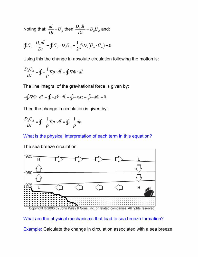
What is the physical interpretation of each term in this equation? The sea breeze circulation

What are the physical mechanisms that lead to sea breeze formation? Example: Calculate the change in circulation associated with a sea breeze

€

d l

Dt=

U a

€

Dad l

Dt= Da

U a

€

U a ⋅

Dad l

Dt∫ =

U a ⋅Da

U a∫ =12

Da

U a ⋅

U a( )∫ = 0

€

DaCa

Dt= −

1ρ∇p ⋅ d

l ∫ − ∇Φ⋅ d

l ∫

€

− ∇Φ⋅ d l ∫ = −g

k ⋅ d l ∫ = −gdz = −dΦ∫ = 0∫

€

DaCa

Dt= −

1ρ∇p ⋅ d

l ∫ = −

1ρ

dp∫

For a barotropic fluid r = r(p) and so:

and absolute circulation is conserved following the motion. This is known as Kelvin’s circulation theorem. What is the relationship between absolute and relative circulation? Ca – absolute circulation Ce – circulation due to the rotation of the Earth C – relative circulation Ca = Ce + C The circulation due to the rotation of the Earth is given by:

, where

is the velocity due to the rotation of the Earth Stokes’ theorem:

,

where is the unit vector normal to the area A and the direction of is defined by the right-hand rule for counterclockwise integration of the line integral. Using Stokes’ theorem we can rewrite our equation for Ce as:

€

−1ρdp∫ = 0

€

DaCa

Dt= 0

€

Ce =

U e ⋅ d l ∫

€

Ue = Ω × r

€

F ⋅ d s ∫ = ∇ ×

F ( ) ⋅ n dA

A∫∫

€

n

€

n

€

Ce =

U e ⋅ d l ∫ = ∇ ×

U e( ) ⋅ n dA

A∫∫

Using the vector identity:

For a horizontal plane is directed in the vertical direction and

, where we have used Then:

,

where Ae is the area projected onto the equatorial plane and: Ae = Asinf Then: C = Ca – Ce = Ca – 2WAsinf = Ca – 2WAe The relative circulation (C) is the difference between the absolute circulation (Ca) and the circulation due to the rotation of the Earth (Ce). Taking of this equation gives:

€

∇ ×

U e( ) =∇ × Ω × r ( ) =∇ ×

Ω × R ( ) =Ω∇ ⋅

R = 2

Ω

€

n

€

∇ ×

U e( ) ⋅ n = 2 Ω ⋅ n = 2Ωsinφ = f

€

Ω =Ωcosφ

j +Ωsinφ

k

Ce = ∇×Ue( ) ⋅ ndA

A∫∫ = 2ΩsinφA = 2ΩAe

€

D Dt

€

DCDt

=DCa

Dt− 2ΩDAe

DtDCDt

= −dpρ

∫ − 2ΩDAeDt

For a barotropic fluid this reduces to:

Integrating from an initial state (1) to a final state (2) gives:

What is the physical interpretation of this result? Vorticity Vorticity – a microscopic measure of rotation at any point in a fluid Vorticity is defined as the curl of the velocity ( ) Absolute vorticity: Relative vorticity:

It is typical to consider only the vertical component of the vorticity vector: Vertical component of absolute vorticity:

Vertical component of relative vorticity:

Under what conditions will z be positive?

€

DCDt

= −2ΩDAeDt

€

C2 −C1 = −2Ω Ae2 − Ae1( )= −2Ω A2 sinφ2 − A1 sinφ1( )

€

∇ ×

V

€

ω a =∇ ×

U a

€

ω =∇ ×

U

€

ω =∇ ×

U =

i j k

∂∂x

∂∂y

∂∂z

u v w

=∂w∂y

−∂v∂z

'

( )

*

+ , i + ∂u

∂z−∂w∂x

'

( )

*

+ , j + ∂v

∂x−∂u∂y

'

( )

*

+ , k

€

η ≡ k ⋅ ∇ ×

U a( )

€

ζ ≡ k ⋅ ∇ ×

U ( ) =

∂v∂x

−∂u∂y

What is the relationship between absolute and relative voriticity? Vertical component of planetary vorticity: Then:

The absolute vorticitiy is equal to the sum of the relative and planetary vorticity. What is the relationship between vorticity and circulation? Consider the circulation for flow around a rectangular area dxdy:

€

k ⋅ ∇ ×

U e( ) = 2Ωsinφ = f

€

η = ζ + f

€

δC = uδx + v+∂v∂xδx

$

% &

'

( ) δy− u +

∂u∂yδy

$

% &

'

( ) δx − vδy

δC =∂v∂x

−∂u∂y

$

% &

'

( ) δxδy

δC = ζδA

ζ =δCδA

We can also relate circulation and vorticity using Stokes’ theorem and the definition of vorticity:

This indicates that the average vorticity is equal to the circulation divided by the area enclosed by the contour used in calculating the circulation. For solid body rotation:

and

In this case the vorticity (z) is twice the angular velocity (W)

€

C =

U ⋅ d l ∫

C = ∇ ×

U ( ) ⋅ n dAA∫∫

C = ζdAA∫∫

C = ζ A

ζ =CA

€

C = 2ΩπR2

€

ζ = 2Ω

Vorticity in Natural Coordinates

From this figure the circulation is:

From the geometry shown in this figure:

, where db is the angular change in wind direction This then gives:

In the limit as :

Noting that then

What is the physical interpretation of this equation?

€

δC =V δs + d δs( )[ ] − V +∂V∂n

δn%

& '

(

) * δs

δC =Vd δs( ) − ∂V∂n

δnδs

€

d δs( ) = δβδn

€

δC =Vδβδn − ∂V∂n

δnδs

δC = V δβδs

−∂V∂n

&

' (

)

* + δnδs

δCδnδs

=V δβδs

−∂V∂n

€

δn,δs→ 0

€

δCδnδs

= ζ =V ∂β∂s

−∂V∂n

€

∂β∂s

=1Rs

€

ζ =VRs

−∂V∂n

Can purely straigthline flow have non-zero vorticity? Where would this occur in the real world? Can curved flow have zero vorticity?

Potential Vorticity Kelvin’s circulation theorem states that circulation is constant in a barotropic fluid. Can we expand this result to apply for less restrictive conditions? Density can be expressed as a function of p and q using the ideal gas law and the definition of q.

and

€

ρ =pRT

€

θ =T psp

#

$ %

&

' (

R cp

⇒ T = θpps

#

$ %

&

' (

R cp

Then:

On an isentropic surface r is only a function of p and the solenoidal term is given by:

Then for adiabatic motion a closed chain of fluid parcels on an isentropic surface satisfies Kelvin’s circulation theorem:

For an approximately horizontal isentropic surface: , where zq is the relative vorticity evaluated on an isentropic surface. Kelvin’s circulation theorem is then given by:

and

following the air parcel motion

€

ρ =pps

R cp

RθpR cp=p 1−R cp( )ps

R cp

Rθ=pcv cp ps

R cp

Rθ

€

dpρ∝ dp 1−cv cp( ) = 0∫∫

€

DCa

Dt=D C + 2ΩδAsinφ( )

Dt= 0

€

C ≈ ζθδA

€

D C + 2ΩδAsinφ( )Dt

=D δA ζθ + 2Ωsinφ( )[ ]

Dt=D δA ζθ + f( )[ ]

Dt= 0

€

δA ζθ + f( ) = Const.

Consider an air parcel of mass dM confined between two q surfaces:

From the hydrostatic equation and :

For dM conserved following the air parcel motion

Then:

where

Using this expression to replace dA in gives:

€

δpδz

= −ρg

€

δM = ρδV = ρδzδA

€

δM = −δpgδA

€

δM = −δpgδA = Const.

€

δA = −δMgδp

= −δθδp

%

& '

(

) * δMgδθ

%

& '

(

) * = Const.( )g −δθ

δp%

& '

(

) *

€

Const.= δMδθ

€

δA ζθ + f( ) = Const.

€

Const.( )g −δθδp

%

& '

(

) * ζθ + f( ) = Const.

Ertel’s Potential Vorticity (P) is defined as:

Ertel’s potential vorticity has units of K kg-1 m2 s-1 and is typically given as a potential vorticity unit (PVU = 10-6 K kg-1 m2 s-1) What is the sign of P in the Northern hemisphere? For adiabatic, frictionless flow P is conserved following the motion. The term potential vorticity is used for several similar quantities, but in all cases it refers to a quantity which is the ratio of the absolute vorticity to the vortex depth.

For Ertel’s potential vorticity the vortex depth is given by

How will change if the vortex depth increases (decreases)? Potential vorticity for an incompressible fluid For an incompressible fluid r is constant and the mass, M, is given by: M = rhdA, where h is the depth of the fluid being considered

Rearranging gives:

And the potential vorticity is given by:

As above, the potential voriticity is constant for frictionless flow following the air parcel motion.

€

P ≡ ζθ + f( ) −gδθδp

'

( )

*

+ ,

€

−δpδθ

€

ζθ + f

€

δA =Mρh

€

ζ + fh

For a constant depth fluid:

(absolute vorticity is conserved following the motion) This puts a strong constraint on the types of motion that are possible. Consider a zonal flow that has z0 = 0 initially so h0 = f0 Since , then at some later time z + f = h0 = f0 For a flow that turns to the north f > f0 and z = f0 – f < 0 For a flow that turns to south f < f0 and z = f0 – f > 0 Can these conditions be satisfied for both easterly and westerly flow?

€

ζ + f =η = Const.

€

ζ + f =η = Const.

For a fluid in which the depth can vary potential vorticity, rather than absolute voriticity, is conserved. Consider westerly flow over a mountain:

Air column

depth Increase

Decrease

Increase

Decrease (return to

original value) Change in

Decrease

Increase

Decrease

Increase (return to

original value)

Change in

Increase

Decrease

Increase

Decrease

Sign of z Positive Negative Positive Negative Resulting

motion northward southward lee side

trough southward

Change in Increase

Decrease

Increase

Decrease

€

δp ↑

€

δp ↓

€

δp ↑

€

δθδp

€

ζ + f

€

f

For easterly flow over a mountain:

Air column

depth Decrease (Return to

original value)

Increase

Decrease

Increase

Change in

Increase

(Return to original value)

Decrease

Increase

Decrease

Change in

Decrease

Increase

Decrease

Increase

Sign of z Zero Positive Negative Positive Resulting

motion westward northward southward southward

Change in

Return to original value

Increase

Decrease

Decrease

As was the case for flows in which absolute vorticity was conserved the flow responds differently for easterly and westerly flow.

€

δp ↓

€

δp ↑

€

δp ↑

€

δθδp

€

ζ + f

€

f

Vorticity Equation We are interested in being able to predict the time rate of change of vorticity without the constraints of adiabatic motion. To do this we will derive the vorticity equation.

Since vorticity is defined as:

We will subtract of the u momentum equation from of the v

momentum equation:

This gives:

Noting that:

the vorticity equation becomes:

€

ζ =∂v∂x

−∂u∂y

€

∂∂y

€

∂∂x

€

∂∂x

∂v∂t

+ u∂v∂x

+ v∂v∂y

+ w∂v∂z

+ fu = −1ρ∂p∂y

%

& '

(

) *

−∂∂y

∂u∂t

+ u∂u∂x

+ v∂u∂y

+ w∂u∂z

− fv = −1ρ∂p∂x

%

& '

(

) *

€

∂ζ∂t

+ u∂ζ∂x

+ v∂ζ∂y

+ w∂ζ∂z

+ ζ + f( ) ∂u∂x

+∂v∂y

$

% &

'

( ) +

∂w∂x

∂v∂z−∂w∂y

∂u∂z

$

% &

'

( ) + v

∂f∂y

=

1ρ2

∂ρ∂x∂p∂y

−∂ρ∂y∂p∂x

$

% &

'

( )

€

DfDt

=∂f∂t

+ u∂f∂x

+ v∂f∂y

+ w∂f∂z

= v∂f∂y

DζDt

=∂ζ∂t

+ u∂ζ∂x

+ v∂ζ∂y

+ w∂ζ∂z

€

D ζ + f( )Dt

= − ζ + f( ) ∂u∂x

+∂v∂y

%

& '

(

) * −

∂w∂x

∂v∂z−∂w∂y

∂u∂z

%

& '

(

) * +

1ρ2

∂ρ∂x∂p∂y

−∂ρ∂y∂p∂x

%

& '

(

) *

This equation indicates that changes in absolute vorticity following the motion is due to a: Convergence term Tilting term Solenoidal term What is the physical interpretation of each of these terms? How will the vorticity change under the influence of convergence? Physical interpretation of the tilting term:

What is the sign of and

in this example? Does this lead to an increase or decrease in absolute vorticity?

€

∂w∂x

€

∂v∂z

The solenoidal term is the microscopic equivalent of the solenoidal term from the circulation theorem. From the circulation theorem the solenoidal term is given by:

Applying Stokes’ theorem to this gives:

Using the vector identity gives:

Expansion of the cross product gives:

Since:

this gives:

€

−dpρ

= − α∇p ⋅ d l ∫∫

€

F ⋅ d s ∫ = ∇ ×

F ( ) ⋅ n dA

A∫∫

&

' (

)

* +

€

− α∇p ⋅ d l ∫ = − ∇ ×α∇p( ) ⋅

k dA

A∫∫

€

∇ ×α∇p =∇α ×∇p

€

− α∇p ⋅ d l ∫ = − ∇α ×∇p( ) ⋅

k dA

A∫∫

€

− ∇α ×∇p( ) ⋅ k = −∂α

∂x∂p∂y

+∂α∂y

∂p∂x

€

∂α∂x

=∂ρ−1

∂x= −

1ρ2

∂ρ∂x

∂α∂y

=∂ρ−1

∂y= −

1ρ2

∂ρ∂y

€

−∂α∂x

∂p∂y

+∂α∂y

∂p∂x

=1ρ2

∂ρ∂x∂p∂y

−1ρ2

∂ρ∂y∂p∂x

Then

Dividing this by the area gives the solenoidal term in the vorticity equation. Vorticity equation in isobaric coordinates

What do each of the terms in this equation represent? In isobaric coordinates there is no solenoidal term. Scale Analysis of the Vorticity Equation We can simplify the vorticity equation through scale analysis. Consider the scales for mid-latitude synoptic weather systems: Horizontal scale U 10 m s-1 Vertical scale W 10-2 m s-1 Length scale L 106 m Depth scale H 104 m Horizontal pressure scale dp 10 hPa Horizontal pressure scale dp/r 103 m2 s-2 Mean density r 1 kg m-3 Fractional density fluctuation dr/r 10-2 Time scale T = L/U 105 s Coriolis parameter F 10-4 s-1 “Beta” parameter b 10-11 m-1 s-1

€

− ∇α ×∇p( ) ⋅ k dA

A∫∫ =

1ρ2

∂ρ∂x∂p∂y

−1ρ2

∂ρ∂y∂p∂x

*

+ ,

-

. / A

€

∂ζ∂t

= − V ⋅∇ ζ + f( ) −ω ∂ζ

∂p− ζ + f( )∇ ⋅

V + k ⋅ ∂

V ∂p

×∇ω)

* +

,

- .

What is the magnitude of b in the mid-latitudes? z scales as:

,

where is used since may partially cancel

What is the relative magnitude of z compared to f0?

,

so z is often an order of magnitude smaller than f0 (the planetary vorticity) Using this we can approximate the convergence term as:

(i.e. we can neglect the relative vorticity contribution to the convergence term)

€

∂f∂y

= β =∂ 2Ωsinφ( )

∂y=∂ 2Ωsin y

a&

' (

)

* +

∂y

β =2Ωacos y

a=2Ωacosφ

€

ζ =∂v∂x

−∂u∂y

<~

UL

~ 10−5 s-1

€

<~

€

∂v∂x

and ∂u∂y

€

ζf0

<~

Uf0L

≡ Ro ~ 10−1

€

− ζ + f( ) ∂u∂x

+∂v∂y

%

& '

(

) * ≈ − f

∂u∂x

+∂v∂y

%

& '

(

) *

This approximation is not valid near the center of intense areas of low pressure where:

and then both relative and planetary vorticity must be considered in the convergence term. What is an example of a type of flow where we cannot neglect z? Scale analysis of the terms in the vorticity equation gives:

Note that is used for the last three terms in this list since portions of each of these terms may partially cancel.

€

ζf~ 1

€

∂ζ∂t

,u∂ζ∂x

,v∂ζ∂y

~ U2

L~ 10−10 s-2

w∂ζ∂z

~ WUL

~ 10−11 s-2

v∂f∂y

~Uβ ~ 10−10 s-2

f ∂u∂x

+∂v∂y

&

' (

)

* + <

~

f0UL

~ 10−9 s-2

∂w∂x

∂v∂z

+∂w∂y

∂u∂z

&

' (

)

* + <

~

WLUH

~ 10−11 s-2

1ρ2

∂ρ∂x∂p∂y

−∂ρ∂y∂p∂x

&

' (

)

* + <

~

δρρδpρ

1L2 ~ 10−11 s-2

€

<~

What is the largest term in the vorticity equation? In order for the vorticity equation to be satisfied:

which implies that the flow must be quasi non-divergent:

How does the magnitude of the divergence compare to the magnitude of the relative and planetary vorticity?

The horizontal divergence is two orders of magnitude smaller than the f and one order of magnitude smaller than z Retaining the largest terms (10-10 s-2) in the vorticity equation gives:

where

What is the physical interpretation of the scaled vorticity equation?

€

f ∂u∂x

+∂v∂y

#

$ %

&

' ( ~ 10−10 s-2 < 10−9 s-2

€

∂u∂x

+∂v∂y

#

$ %

&

' ( ~ 10−6 s-1 <

UL

~ 10−5 s-1

€

∂u∂x

+∂v∂y

#

$ %

&

' ( f0 <

~

10−6 s-1

10−4 s-1 ~ 10−2 ~ Ro2

∂u∂x

+∂v∂y

#

$ %

&

' ( ζ <

~

10−6 s-1

10−5 s-1 ~ 10−1 ~ Ro

€

∂ζ∂t

+ u∂ζ∂x

+ v∂ζ∂y

+ v∂f∂y

= − f ∂u∂x

+∂v∂y

%

& '

(

) *

Dh ζ + f( )Dt

= − f ∂u∂x

+∂v∂y

%

& '

(

) *

€

Dh

Dt≡∂∂t

+ u ∂∂x

+ v ∂∂y

Near the center of intense low pressure systems, where z and f have similar magnitude the scaled vorticity equation becomes:

Why can cyclonic systems become more intense than anticyclonic systems? This is consistent with our analysis of the gradient wind equation where we found that the intensity of high pressure systems was limited while the intensity of low pressure systems was not. Is the scaled vorticity equation appropriate in the vicinity of fronts? Near fronts: L~105 m and W~10-1 m s-1 Using these scales indicates that the vertical advection, tilting, and solenoidal terms in the vorticity equation may all be as large as the divergence term, and thus must all be retained. Vorticity in Barotropic Fluids Barotropic (Rossby) Potential Vorticity Equation Consider an atmosphere that is: Barotropic: r = r(p)

Incompressible:

With a depth h(x,y,t) = z2 – z1, where z2 and z1 are the heights of the upper and lower boundaries of the atmosphere

€

Dh ζ + f( )Dt

= − ζ + f( ) ∂u∂x

+∂v∂y

%

& '

(

) *

€

DρDt

= 0

For an incompressible fluid the continuity equation is:

Then the scaled vorticity equation becomes:

Approximating the vorticity (z) by the geostrophic vorticity (zg), where

gives:

In a barotropic fluid does not vary with height and the equation above can be integrated from height z1 to z2 to give:

Noting that gives:

€

∇ ⋅

U = 0∂u∂x

+∂v∂y

= −∂w∂z

€

Dh ζ + f( )Dt

= − ζ + f( ) ∂u∂x

+∂v∂y

%

& '

(

) * = ζ + f( )∂w

∂z

€

ζg =∂vg∂x

−∂ug∂y

€

Dh ζg + f( )Dt

= ζg + f( )∂w∂z

€

V g

€

Dh ζg + f( )Dt

∂zz1

z2

∫ = ζg + f( )∂wz1

z2

∫

Dh ζg + f( )Dt

z2 − z1( ) = ζg + f( ) w z2( ) − w z1( )[ ]

hDh ζg + f( )

Dt= ζg + f( ) w z2( ) − w z1( )[ ]

€

w ≡ DhzDt

and

so

Then:

Rossby potential vorticity: The Rossby potential vorticity is conserved following the motion. Barotropic Vorticity Equation For a barotropic, incompressible fluid with purely horizontal flow (w = 0) the vorticity equation becomes:

and the absolute vorticity (z + f) is conserved following the motion.

€

w z1( ) =Dhz1Dt

€

w z2( ) =Dhz2Dt

€

w z2( ) − w z1( ) =Dhz2Dt

−Dhz1Dt

=Dh z2 − z1( )

Dt=DhhDt

€

hDh ζg + f( )

Dt= ζg + f( )Dhh

Dt1

ζg + f( )Dh ζg + f( )

Dt=1hDhhDt

Dh ln ζg + f( )Dt

=Dh lnhDt

Dh ζg + f( ) h[ ]Dt

= 0

€

ζg + f( ) h

€

Dh ζ + f( )Dt

= − ζ + f( )∂w∂z

= 0

A more general result is that for a flow that has non-divergent horizontal

winds :

For a non-divergent flow the wind can be represented by a streamfunction

such that:

Example: Show that with this definition of the streamfunction the horizontal wind is non-divergent. The relative vorticity is then given by:

The vorticity equation can then be written as:

,

What is the physical interpretation of this equation? This equation can be solved numerically to predict the time evolution of y. V and z can then be calculated from y.

€

∂u∂x

+∂v∂y

= 0#

$ %

&

' (

€

Dh ζ + f( )Dt

= 0

€

ψ x,y( )[ ]

€

V ψ ≡

k ×∇ψ = −

∂ψ∂y i + ∂ψ

∂x j = u i + v j

€

ζ =∂v∂x

−∂u∂y

=∂ 2ψ∂x2

+∂ 2ψ∂y2

≡ ∇ 2ψ

€

Dh ζ + f( )Dt

= 0

Dh ∇ 2ψ + f( )Dt

=∂∇ 2ψ∂t

+

V ψ ⋅∇ ∇ 2ψ + f( ) = 0

∂∇ 2ψ∂t

= −

V ψ ⋅∇ ∇ 2ψ + f( )

The flow in the mid-troposphere (~500 mb) is often nearly non-divergent and this equation can be used to produce a reasonable prediction of the time evolution of the flow at this level. Baroclinic (Ertel) Potential Vorticity Equation Ertel potential vorticity is given by:

and is conserved following the motion for adiabatic, frictionless flow. We want to derive an equation for the time evolution of P in the presence of diabatic effects and friction. This equation can be derived by rewriting the horizontal momentum equation in isentropic coordinates. We can use q as a vertical coordinate in a stably stratified atmosphere since and q is a monotonic function of height. The vertical velocity in isentropic coordinates is defined as:

When will ? For an air parcel with mass dM:

,

where is the density in (x,y,q) space

€

P ≡ ζθ + f( ) −g∂θ∂p

'

( )

*

+ ,

€

∂θ ∂z > 0

€

˙ θ ≡DθDt

€

˙ θ = 0

€

δM = ρδAδz = δA −δpg

%

& '

(

) * =

δAg

−∂p∂θ

%

& '

(

) * δθ =σδAδθ

€

σ = −1g∂p∂θ

Then the governing equations in isentropic coordinates are given by: Horizontal momentum equation in isentropic coordinates:

,

where is the Montgomery streamfunction Continuity equation in isentropic coordinates:

Hydrostatic equation in isentropic coordinates:

,

where P is the Exner function Isentropic vorticity equation:

,

where is the total derivative following the horizontal motion

on an isentropic surface The continuity equation can be rewritten as:

€

∂

V ∂t

+∇θ

V ⋅ V

2+ Ψ

'

( )

*

+ , + ζθ + f( )

k ×

V = − ˙ θ ∂ V ∂θ

+ F r

€

Ψ = cpT +Φ

€

∂σ∂t

+∇θ ⋅ σ V ( ) = −

∂ σ ˙ θ ( )∂θ

€

∂Ψ∂θ

= Π p( ) ≡ cppps

'

( )

*

+ ,

R cp

= cpTθ

€

˜ D ζθ + f( )Dt

+ ζθ + f( )∇θ ⋅ V = k ⋅∇θ ×

F r − ˙ θ

∂ V ∂θ

)

* +

,

- .

€

˜ D Dt

=∂∂t

+ V ⋅∇θ

€

˜ D σ −1

Dt−σ −1∇θ ⋅

V =σ −2 ∂ σ

˙ θ ( )∂θ

Ertel potential vorticity equation

,

where Ertel’s potential vorticity is given by What is the physical interpretation of this equation?

For adiabatic, frictionless flow and P is conserved following the

motion.

€

˜ D PDt

=∂P∂t

+ V ⋅∇θ P =

Pσ

∂ σ ˙ θ ( )∂θ

+σ −1 k ⋅∇θ × F r − ˙ θ

∂ V ∂θ

)

* +

,

- .

€

P = ζθ + f( ) σ

€

˜ D PDt

= 0