Discussion Papers are a series of manuscripts in their draft form. They are not intended for

circulation or distribution except as indicated by the author. For that reason Discussion Papers may

not be reproduced or distributed without the written consent of the author.

CIRJE-F-101

A New Composite Index ofCoincident Economic Indicators in Japan:

How Can We Improve the Forecast Performance?Shin-ichi Fukuda

University of TokyoTakashi Onodera

Nihon Keizai Shimbun, Inc.

January 2001

A New Composite Index of Coincident Economic Indicators in Japan:

How can we improve the forecast performance? *

Shin-ichi Fukuda **

Faculty of Economics, The University of Tokyo

and

Takashi Onodera

Electronic Media Bureau, Nihon Keizai Shimbun, Inc.

Abstract

The purpose of this paper is to construct a new composite index of coincident economic indicators in

Japan and to demonstrate their usefulness in forecasting recent short-run economic fluctuations.

The method of construction is based on the single-index dynamic factor model. Our two types of

indexes are highly correlated with the traditional composite index compiled by the EPA over

business-cycle horizons. However, standard leading indicators, which failed to forecast the

traditional composite index, make a satisfactory performance in forecasting our indexes in the 1990s.

In addition, lagged values of our indexes help to improve the leading indicators’ performance in

forecasting the traditional composite index in the 1990s. The result is noteworthy because a large

number of research institutes made serious errors in forecasting recent recessions in Japan.

Key Words: Business cycles, Composite indicators, Macroeconomic forecasting, Kalman filter

* The authors wish to thank two anonymous referees, S. Saruyama, I. Nakagome, Y. Honda, and

other seminar participants at Japan Center for Economic Research for helpful comments and

suggestions. Fukuda’s research is supported by Japanese Government, Ministry of Education Aid

for Science Research on Priority Area (B) #12124203.

** Address any correspondence to Shin-ichi Fukuda: Faculty of Economics, The University of

Tokyo, Hongo Bunkyo-ku, Tokyo 113-0033, Japan (E-mail: sfukuda@e.u-tokyo.ac.jp).

2

1. Introduction

The composite index of coincident economic indicators (henceforth, CI) in Japan, currently

compiled by the Economic Planning Agency (EPA), is designed to measure the state of overall

economic activity in Japan. Putting aside some details, the compiling procedure is essentially the

same as that in the United States. The compiled index in Japan is, however, different from the U.S.

index in that it reflects larger number of macroeconomic variables than the CI in the United States.1

Loosely speaking, the index is constructed as a simple average of the growth rates of eleven key

macroeconomic time series.2 Table 1 is a list of eleven key macroeconomic time series that are

currently compiled for the CI in Japan. These variables include several variables related to

“industrial production”, three variables related to “trade sales”, and two variables related to

“employment”. However, these variables do not include the data on personal income that is one

of the major components in the CI in the United States.3 In addition, since nearly half of the

compiled variables are closely correlated with the index of industrial production, the simple average

might cause a bias that the CI’s movements are dominated by the industrial production index in

Japan.

The purpose of this paper is to construct a new composite index of coincident economic

indicators in Japan and to explore their usefulness in forecasting short-run economic fluctuations in

the 1990s. The method of construction is based on the single-index dynamic factor model that is

originally formulated by Stock and Watson (1989, 1991). The model follows the notion that the

co-movements in many macroeconomic variables have a common factor that can be captured by a

1 The Index of Coincident Economic Indicators in the United States, formerly compiled by the U.S.

Department of Commerce and currently maintained by the Conference Board, is constructed as a

weighted average of four key macroeconomic variables such as Industrial Production, Personal

Income, MFG & Trade Sales, and Employees on Non-agriculture Payrolls. 2 Strictly speaking, before the index is constructed as a simple average, eleven macroeconomic time

series are transformed and smoothed out. 3 One exceptional study that discussed arbitrariness in choosing the EPA’s coincident indicators in

Japan is Kano (1990).

3

single unobservable variable. In the estimation, we present a parametric model where a single

index, Ct, is an unobserved variable common to monthly macroeconomic time series. Because the

model is linear in the unobserved variable, the Kalman Filter can be used to construct the likelihood

function and thereby to estimate the new index of coincident indicators, Ct, in Japan.

The compiled data series are a part of the data set used to construct the CI compiled by the EPA

(henceforth, the EPA-CI). In the estimation, we constructed two types of indexes: type 1 index

that has a moderate correlation with the industrial index, and type 2 index that has a significant

correlation with the industrial production index. Despite compiling smaller number of data series,

our two types of indexes are highly correlated with the EPA-CI over business-cycle horizons. A

graphical comparison showed that the EPA-CI had more clear-cut ups and downs. However, the

EPA-CI series failed to detect some turning points, particularly the turning point in February 1991.

In contrast, our two types of indexes succeed in detecting the turning point in February 1991.

Comparing the performances of the composite indexes of coincident indicators, we investigate

how well several leading indicators can forecast alternative indexes of coincident indicators. A

particular interest of our exercise is to examine how we can improve forecast performances in the

1990s. In terms of economic forecasts in Japan, the 1990s was a special decade because public

and private research institutes made serious errors in forecasting business cycles and prolonged

recessions. For example, following Yamasawa et al. (1998), Figure 1 summarizes forecast

performances of major private research institutes in Japan since the 1970s. It plots the actual

growth rates of real GDP in Japan and the maximums, minimums, and averages of their forecasted

values. From the figure, we can easily see that the performances became poorer in the 1990s and

frequently failed to detect booms and recessions in the 1990s.4 This indicates that it is now urgent

to invent new indexes that help to improve forecast performances of leading indicators in Japan

since the 1990s.

In the paper, we first show that in forecasting various indexes of coincident indicators, standard

leading indicators performed well until the 1980s but that their performances became unsatisfactory

in the 1990s. In particular, we demonstrate that the performances of the standard leading

4 On causes of the long stagnation of Japan during the 1990s, see, for example, Bayoumi (1999),

Hoshi and Kashyap (2000), and Motonishi and Yoshikawa (1999).

4

indicators in forecasting the EPA-CI drastically deteriorated in the 1990s. However, we find that

the standard leading indicators still satisfactorily forecast our two types of indexes, even in the 1990s.

This implies that our new CIs have a stable relation with standard leading indicators. In addition,

when the lagged values of our indexes are included in multivariate leading indicator forecasts, they

could improve the performances in forecasting the EPA-CI even in the 1990s.

Needless to say, our approach is not the only way to construct a composite index of coincident

indicators. In fact, even focusing on factor models, a large number of studies proposed several

sophisticated methods and constructed different types of indexes in the United Sates.5 In addition,

our approach uses no filter other than the first-difference filter and allows no regime switch in the

model.6 However, in Japan, there were only limited attempts to construct a composite index of

coincident indicators based on a dynamic factor model in the 1990s. Among these limited studies,

Ohkusa (1992) and Mori et al. (1993) are the first attempts to apply the Stock-Watson method to the

Japanese economy. 7 They constructed the Stock-Watson type index in Japan based on annual

growth rates of four macroeconomic variables. But since their sample period was from January

1975 to October 1991, it is still far from clear what implications the Stock-Watson type index has on

the Japanese economy in the 1990s that is the main concern in the paper.

The paper proceeds as follows. Section 2 presents the single-index model by which our two

types of indexes are constructed in the following sections. Section 3 explains the data for our

empirical analysis. Section 4 examines how the constructed indexes are correlated with other

coincident indicators. Section 5 investigates performances of leading indicators in forecasting the

5 Factor models were generalized to dynamic environments by Sargent and Sims (1977), Geweke

(1977), and Watson and Engle (1983). Some recent contributions after Stock and Watson’s seminal

studies include Quah and Sargent (1993) and Diebold and Rudebusch (1996), among others. 6 For general survey, see Stock and Watson (1999). Among others, see also Hodrick and Prescott

(1980) and Baxter and King (1999) for more general filters and Hamilton (1989) and Kim and

Nelson (1999) for regime switch models. 7 In addition, NLI Research Institute made a preliminary estimate of the Stock-Watson type index in

Japan, and Japan Center for Economic Research constructed “Jcer Business Index” by the principal

component analysis.

5

coincident indexes. Section 6 summarizes our main results and refers to some possible

extensions.

2. The Single-Index Model

Let yi,t (i = 1, 2, …, M) denote the logarithm of a macroeconomic time-series variable that is

supposed to move contemporaneously with overall economic conditions. We assume that all of

the coincident series yi,t (i = 1, 2, …, M) have a unit root but that there is no co-integration among

these variables. Then, in terms of the changes of the variables, the single-index model is

formulated as follows.

(1) ∆yi,t = βi + γi ∆Ct + ui,t , (i = 1, 2, …, M)

(2) ∆Ct = φ1∆Ct-1 + φ2∆Ct-2 + … + φp∆Ct-p + ηt,

(3) ui,t = di,1ui,t-1 + di,2ui,t-2 + … + di,qui,t-q + εi,t, (i = 1, 2, …, M)

where ∆yi,t ≡ yi,t - yi,t-1.

The above single-index model states that the growth rate of the i-th macroeconomic variable, ∆yi,t,

consists of two stochastic components: the common unobserved scalar “index” ∆Ct and a

idiosyncratic shock, ui,t (i = 1, 2, …, M). Both the unobserved index and the idiosyncratic shocks

are modeled as having autoregressive stochastic processes, AR(p) in equation (2) and AR(q) in

equation (3), respectively.

Equation (2) implies that the mean of ∆Ct is implicitly assumed to be zero in the model. We

imposed the identifying constraint assuming that ∆Ct is represented as a deviation form. For a

normalization, the scale of ∆Ct is identified by setting var(ηt) = 1. Finally, we assume that ui,t and

∆Ct are mutually uncorrelated at all leads and lags for all i = 1, 2, …, M.

In estimating the above single-index model, we transform (1)-(3) into a state space form so that

the Kalman Filter can be used to evaluate the likelihood function. The state space form has both

the state equation and the measurement equation. The measurement equation relates the observed

variables, ∆yi,t (i = 1, 2, …, M), to the unobserved state vector which consists of ∆Ct, ui,t, Ct-1, and

6

their lags. The state equation describes the evolution of the state vector.

For example, when M = 5, p = 3, and q = 1, the measurement equation and the state equation are

respectively given by

(4)

∆∆∆

=

∆∆∆∆∆

−

−

−

1

,5

,4

,3

,2

,1

2

1

5

4

3

2

1

,5

,4

,3

,2

,1

0100000000100000000100000000100000000100

t

t

t

t

t

t

t

t

t

t

t

t

t

t

cuuuuuccc

yyyyy

γγγγγ

(5)

+

∆∆∆

=

∆∆∆

−

−

−

−

−

−

−

−

−

−

−

−

0

00

1000000010000000000000000000000000000000000000000000000010000000001000000

,5

,4

,3

,2

,1

2

1,5

1,4

1,3

1,2

1,1

3

2

1

1,5

1,4

1,3

1,2

1,1

321

1

,5

,4

,3

,2

,1

2

1

t

t

t

t

t

t

t

t

t

t

t

t

t

t

t

t

t

t

t

t

t

t

t

t

vvvvv

cuuuuu

ccc

dd

dd

d

cuuuuuccc εφφφ

Assuming that M = 5, p = 3, and q = 1, the following analysis uses the Kalman Filter to construct

the likelihood function of this state space form and to estimate the new index of coincident indicators,

Ct. Estimates based on the entire sample are computed both with and without Kalman smoother.

3. The Data for the Empirical Analysis

The purpose of this section is to explain the choice of data series to construct a new composite

7

index of coincident economic indicators in Japan. All candidates of our data series are from the

monthly data that are used to construct the CI compiled by the Economic Planning Agency in Japan

(henceforth, the EPA-CI). The data series reflect recent substantial revisions of industrial

production indexes in Japan.8 When the published data series are seasonally unadjusted, we

transformed them into seasonally adjusted series by the Census-X11. Since ten monthly series are

available, one possible choice for our data set might be to use all of these ten macroeconomic

variables.9 However, the use of ten macroeconomic variables is not only computationally costly

but also might cause biases for the following two reasons.

First, nearly half of these variables are highly correlated with “Index of Industrial Production”

(IIP95P). For example, Table 2 summarizes contemporaneous cross correlations among the

growth rates of the ten variables over the period 1973:2-1999:12. In the table, “Index of Industrial

Production” (IIP95P) has large positive correlations with four variables: “Index of Raw Materials

Consumption” (IIP95M), “Index of Operating Rate” (IIP95O), “Index of Producers' Shipments,

Investment Goods” (IIP95S), and “Sales of Small and Medium Size Companies” (SMSALE). It

also has correlations of about 0.5 with “Electric Power Consumption of Large Users” (CELL9) and

“Index of Wholesale Sales” (SCI95). This indicates that the use of these macroeconomic

variables, particularly the first four variables, might cause a bias that the constructed CI tends to be

dominated by the movements of industrial production.

Secondly, except for two employment variables, these monthly macroeconomic variables are

highly volatile and their growth rates have significant negative serial correlations over time. For

example, Table 3 summarizes how large the serial correlations of the growth rates of the ten

macroeconomic variables were in Japan over the period 1973:2-1999:12. It also reports the size

of a serial correlation the growth rates of industrial production index had in the United States over

the period 1975:1-2000:7. The results in Japan show that except for two labor market variables

(that is, HWINMF and ESRAO), the macro variables in Japan have significant negative serial

correlations in their growth rates. Among these eight variables, growth rates of “Index of

8 Following the revision, historical data series of the EPA-CI were also revised. 9 Although the EPA-CI is constructed by eleven macroeconomic variables listed in Table 1,

“Business Profit” is quarterly data.

8

Industrial Production” (IIP95P) have the third largest negative serial correlation. The result is in

marked contrast with industrial production index in the United States because it shows a significant

positive serial correlation in table 3. Recalling that the majority of the compiled data has large

contemporaneous correlations with IIP95P, this indicates that short-term volatility of the EPA-CI is

largely attributable to the highly volatile time-series property of the industrial production index in

Japan.

Because of these reasons, the following analysis selectively compiles five from among the ten

variables to estimate smoother and less biased indexes. The basic principle in selecting the series

is not only to use “industrial production index (IIP95P)” but also to use a variable related to “trade

sales” and a variable related to “labor market”. The principle comes from the fact that with a few

exceptions, these two types of variables have smaller contemporaneous cross correlations with

“IIP95P” and are less volatile than “IIP95P”.10 In addition, these two variables as well as

“IIP95P” are key variables in constructing the CI in the United States.11

Unless specified, the sample period of the monthly data is from 1973:2 to 1999:12 and all of the

data are obtained from the Nikkei NEEDS database.12 We specifically compile five time series

from the following two types of data sets.

Type 1 data set: (1) IIP95P, (2) SCI95, (3) ESRAO, (4) HWINMF, (5) CELL9.

10 For example, Table 2 shows that “Index of Non-scheduled Hours Worked” (HWINMF) and

“Ratio of Job Offers to Applicants” (ESRAO) have smaller correlation with “Index of Industrial

Production”, although each correlation is significantly positive, that is, about 0.3. In addition,

“Sales of Department Stores” (SDS) have little correlation with most of the variables, although they

have small correlation with “Index of Wholesale Sales” and “Sales of Small and Medium Size

Companies”. Thus, compiling these data series, we may construct a balanced CI where the

industrial production index does not have a dominant effect on it. 11 However, because of the lack of the data in the EPA’s series, we do not include the data on

“personal income” that is another component of the CI in the United States. 12 The sample period starts from 1973:2 because SCI95 and SMSALE are available only from

1973:1.

9

Type 2 data set: (1) IIP95P, (2) SMSALE, (3) HWINMF, (4) IIP95O, (5) IIP95M.

(See table 1 for the definitions of these variables.)

Both data sets satisfy the basic principle explained above. However, the type 1 data set was

chosen so as to include variables that are less correlated with IIP95P in Table 2. In addition, the

type 1 data set includes two employment variables both of which have significant positive serial

correlations in their growth rates. On the other hand, the type 2 data set was chosen so as to

include variables that have relatively larger correlations with IIP95P in Table 2. Except for

HWINMF, the variables in the type 2 data set have significantly negative serial correlations in their

growth rates.

As we show in the appendix, the Augmented Dickey-Fuller unit root test cannot reject the

hypothesis that the logarithm of each variable has a unit root at the 5% significance level in both data

sets. In addition, except for SMSALE, the Engle-Granger test cannot reject the hypothesis of no

cointegration among these variables at the 10% level. Even for SMSALE, we cannot reject no

cointegration at the 1% level. We thus estimate the single index model by using the logged series

in these data sets.

In both of these data sets, the errors uti are modeled as an AR(1), that is, q=1, for all i, and a third

order autoregressive specification was adopted for ∆Ct, that is, p=3.13 The parameters were

estimated over the period 1973:2-1999:12. The estimated parameters imply that ∆Ct satisfies the

following time-series properties.

For the type 1 data set with Kalman smoother:

(6a) ∆Ct = 0.265*∆Ct-1 + 0.100*∆Ct-2 + 0.257*∆Ct-3,

(0.054) (0.055) (0.052)

13 We tried a fourth order autoregressive specification for ∆Ct, that is, p=4. However, in both data

sets, the coefficients on the fourth order terms were not statistically significant. In addition,

preliminary test statistics showed little evidence that the errors uti are modeled as an AR(2), that is,

q=2, although the evidence was marginal for ESRAO.

10

for the type 1 data set without Kalman smoother:

(6b) ∆Ct = 0.151*∆Ct-1 + 0.132*∆Ct-2 + 0.379*∆Ct-3,

(0.052) (0.052) (0.052)

for the type 2 data set with Kalman smoother:

(7a) ∆Ct = -0.109*∆Ct-1 + 0.221*∆Ct-2 + 0.319*∆Ct-3,

(0.053) (0.052) (0.053)

for the type 2 data set without Kalman smoother:

(7b) ∆Ct = -0.126*∆Ct-1 + 0.252*∆Ct-2 + 0.323*∆Ct-3,

(0.053) (0.051) (0.053)

where standard errors are in the parentheses.

Equations (6a, b) and (7a, b) state that in each data set, ∆Ct follows a statistically significant third

order autoregressive model. The time-series properties look similar regardless of the choice of

Kalman smoother. However, comparing the above AR(3) processes, we can see that ∆Ct has a

positive serial correlation for the type 1 data set but has a negative serial correlation for the type 2

data set. This probably reflects the fact that the type 1 data set includes two labor market

variables that have significantly positive serial correlations in their growth rates, while most of

variables in the type 2 data set have significantly negative serial correlations in their growth rates.

4. The Correlations of the Estimated Indexes with Other Indexes

4.1. The compiled data series

The purpose of this section is to examine how our estimated indexes are correlated with other

11

coincident economic indicators. We first investigate how well each of our estimated indexes

could capture a common factor of the compiled coincident economic indicators. For the total

sample period (1973:2-1999:12) and three sub-sample periods (1973:2-1980:12, 1981:1-1989:12,

1990:1-1999:12), Table 4 summarizes contemporaneous cross correlations of ∆Ct with the growth

rates of five data series that are used to construct ∆Ct.

In the case of the type 1 data set, ∆Ct has relatively balanced correlations with five coincident

economic indicators. Throughout the periods, ∆Ct keeps significant correlations with the growth

rate of IIP95P (the industrial production index) as well as CELL9 (electric power consumption).

The correlations lie in a range between 0.6 and 0.8, although they tend to be smaller when Kalman

smoother is used. However, ∆Ct also has significant correlation with the growth rates of two

employment data, ESRAO and HWINMF, except in the 1980s. Regardless of the choice of

Kalman smoother, the correlations for the total sample period are 0.65 and 0.71 respectively, both of

which are almost equal to the correlation between ∆Ct and the growth rate of IIP95P. This implies

that in the type 1 data set, the industrial production index (IIP95P) does not have a dominant effect

on the movements of ∆Ct.

In contrast, in the case of the type 2 data set, ∆Ct generally has very large correlations only with

IIP95P, IIP95O, and IIP95M. The correlations are greater than 0.9 in most of the periods.

However, ∆Ct has only a mild correlation with HWINMF (the index of non-scheduled hours

worked). Recalling that IIP95P is highly correlated with both IIP95O and IIP95M but is less

correlated with HWINMF, this implies that the industrial production index has a dominant effect on

the movements of a common factor ∆Ct in the type 2 data set.

4.2. The EPA-CI

We next examine how similar our indexes of coincident economic indicators are to the CI

compiled by the Economic Planning Agency in Japan (the EPA-CI). For the total sample period

(1973:2-1999:12) and three sub-sample periods (1973:2-1980:12, 1981:1-1989:12, 1990:1-1999:12),

Table 5 summarizes contemporaneous cross correlations of each of our index ∆Ct with the growth

rates of the EPA-CI. From the table, we can see that for all of our indexes, the correlations are

nearly equal to 0.9. The correlations tend to be high when we compute the index without Kalman

smoother, particularly in the type 1 data set. Comparing the different sample periods, the

12

correlations are highest in the 1970s. However, the correlations are still greater than 0.8 even in

the other sub-periods.

The high correlations with the EPA-CI are particularly noteworthy for the type 1 index because

the type 1 index is less correlated with the industrial production index than the type 2 index and the

EPA-CI. This may imply that there exists a common factor of business cycles that is not

necessarily highly correlated with the industrial production index in Japan.

Graphical comparisons also reconfirm very high correlations of our indexes and the EPA-CI.

For example, Figures 2A-2B respectively plotted the rescaled series of our two types of indexes with

and without Kalman smoother by bold lines and the EPA-CI series by a thin line. In both figures,

the contraction periods are expressed by shaded areas. From the figures, we can see that our two

types of indexes and the EPA-CI exhibit essentially similar ups and downs regardless of the choice

of Kalman smoother.

Among four indexes, the type 2 index without Kalman smoother looks most similar to the EPA-CI,

although it shows large short-run volatility. On the other hand, the type 2 index with Kalman

smoother and the type 1 indexes are stable throughout the periods. In particular, even without

Kalman smoother, the type 1 index shows stable cycles, particularly in the 1990s. This reflects

the fact that the type 1 index has a larger correlation with two stable time series in the labor market

(i.e., HWINMF and ESRAO), while the type 2 index and the EPA-CI have larger correlations with

the industrial production index that is highly volatile in the short-run.

In general, the EPA-CI seems to have more clear-cut ups and downs than our indexes. However,

the EPA-CI series failed to detect some turning points, particularly the turning points in February

1991 and in October 1993.14 In contrast, all of our indexes succeed in detecting the turning point

in February 1991, although they failed to detect the bottom in October 1993.

5. Performances of Leading Indicators in Forecasting the Coincident Indexes

14 The turning points of business cycles have been judged by the committee members appointed by

the Economic Planning Agency in Japan.

13

5.1 The benchmark equation

The purpose of this section is to investigate how well various types of coincident indicators could

be forecasted by several leading indicators. A particular interest of our exercise is to examine

whether standard leading indicators in Japan had satisfactory performances in forecasting various

coincident indicators in the 1990s. The exercise is important because we experienced serious

errors in forecasting business cycles during this period in Japan.

The following exercise focuses on forecasting six-month growth rates of three coincident indexes

(zj,t; j = 1,2,3): the EPA-CI and our two types of indexes without Kalman smoother.15 In the

exercise, we compare the performances of several multivariate regression-based forecasts using

leading indicators. The data series of the leading indicators are the monthly data series that are

used to construct the leading CI compiled by the Economic Planning Agency in Japan. Table 6 is

a list of ten monthly macroeconomic time series that are currently compiled for the CI of leading

indicators in Japan.16 They include not only several indexes related to industrial production but

also a variety of variables such as money supply, business survey, and so on.

The estimated multivariate leading indicator forecasts are of the form

(8) ln(zj, t+6/zj, t) = αj + ∑ ∑= = −kq

hi itqiqj w1 1 ,,,δ +∑ = −−−

mi itjitjij zz1 1,,, )/ln(γ + vj, t,

where {wq,t} are leading indicators that are used to forecast six-month growth rates of a coincident

index, zj,t; j = 1,2,3.

For leading indicators wq,t’s, we took the growth rates of the leading indicators if not already in

rates. We also included lagged values of the dependent variables as predictors. Assuming that

h = 3 and m = 6, the coefficients of (8) were estimated by OLS. Unless specified, the sample

period of the data is from 1974:3 to 1999:12 and all of the data are obtained from the Nikkei NEEDS

15 Since indexes with Kalman smoother exploits future information, we did not use them in the

following forecasts. 16 “Judgement Survey of Small and Medium Size Companies” (SMFTA) is also included in the

leading indicators of the EPA. But since it is quarterly data, we did not use it in our analysis.

14

database. In forecasting six-month growth rates in the 1990s, we implemented both in-sample

forecast based on the parameters estimated over 1974:3 to 1999:12 and out-of-sample forecast based

on the parameters estimated over 1974:3 to 1989:12.

We first tentatively estimated the benchmark equation by using all of ten monthly leading

indicators, that is, k = 10. However, regardless of the choice of the data set, three leading

indicators were never statistically significant with any lags.17 We thus dropped these three

variables and re-estimated the benchmark equation by using the other seven leading indicators:

“Index of Producers' Inventory Ratio to Shipments” (IIP95R), “Index of Raw Materials Inventory”

(IIP95T), “New Job Offers” (ESNOP), “Orders Received for Machinery” (ONMPE), “Building

Construction Starts” (ICVMCS), “Nikkei Commodity Index” (CJ&V), and “Money Supply”

(MNQMACD).

5.2 Forecast performances

In the estimates for the total sample period over 1974:3 to 1999:12, performances of these seven

leading indicators were quite well in forecasting any of three types of coincident indexes. For

example, Table 7 reports the goodness of fit of the simulated in-sample forecasting experiments with

and without lagged dependent variables ln(zj,t-i/zj,t-1-i). It states that regardless of the type of

coincident index, seven leading indicators explained nearly 60% of the total variations when lagged

dependent variables were included in (8). Even without lagged dependent variables, the leading

indicators could explain more than half of fluctuations of all coincident indexes.

However, comparing the forecast performances of the EPA-CI for different sample periods, we

can find that performances of these seven leading indicators were deteriorated significantly in the

1990s for both in-sample and out-of-sample forecasts. For example, Table 8 summarizes the

mean squared errors (MSEs) of the candidate forecasting model for two sub-sample periods,

1976:1-1989:12 and 1990:1-1999:12, and their relative values (i.e., (2)/(1)).18 Comparing the

17 These three indicators are “New Dwelling Construction Started” (ICRFS), “Registration and

Notification of New Motor Vehicles” (JINVPT), and “Index of Investment Environemnts, Mfg.”

(IVIMF). 18 Reflecting the fact that the type 1 index is much smooher than other indexes, its MSEs are much

15

MSEs of the two sub-sample periods, we can easily see that the MSEs of the EPA-CI in

1990:1-1999:12 became much larger than the MSEs in 1976:1-1989:12. Even using in-sample

forecast, the MSE of the EPA-CI was almost doubled in the 1990s. This implies that there was a

substantial structural change in the forecasting model of the EPA-CI in the 1990s.

The result is consistent with the evidence that not a few research institutes in Japan made serious

errors in forecasting business cycles in the 1990s. One possible reason for the poor forecast

performances by the leading indicators may be attributable to the role of unexpected credit crunch

that caused a deep recession in the late 1990s. One may also point out the fact that standard

leading indicators do not include government expenditures that were continuously expanded

throughout the 1990s except in 1997.

However, compared with the EPA-CI, our two types of indexes have relatively modest rises of the

MSEs in the 1990s for both in-sample and out-of-sample forecasts. Even in out-of-sample

forecasts, we see that the rises of the MSEs in the 1990s were relatively small, that is, 1.46 for the

type 1 index and 1.33 for the type 2 index in Table 8.

In addition, when we additionally include lagged values of our indexes in (8), we can see that the

benchmark model can improve its performance even in forecasting six-month growth rates of the

EPA-CI in the 1990s. For example, Table 9 reports how lagged values of our indexes will

improve the performances of the benchmark model in forecasting six-month growth rates of the

EPA-CI. Although the inclusion of lagged values of our indexes in the benchmark models could

reduce the MSEs for some extents, the declines of the MSEs are relatively modest when lagged type

2 indexes are included. However, when lagged type 1 indexes are included, the EPA-CI showed a

substantial decline of the MSEs, particularly in 1990:1-1999:12.

It probably needs further researches to explain why our type 1 index could achieve such a

substantial improvement in forecasting the EPA-CI in the 1990s. However, we may conjecture

that a superior performance of the type 1 index in the 1990s might be attributable to the fact that the

type 1 index incorporates more information that is not related with the industrial production index.

Recalling that the Japanese economy underwent substantial changes of industrial structures in the

1990s, it is highly possible that the EPA-CI, whose movements are dominated by the industrial

smaller in the absolute values.

16

production index, became less relevant to capture business cycles in Japan. In such a case, our

type 1 index could have an important information content in forecasting business cycles in the 1990s,

including the cyclical movements of the EPA-CI.

6. Conclusions

This paper constructed a new composite index of coincident economic indicators in Japan and

demonstrated their usefulness in forecasting the short-run economic growth in the 1990s. The

traditional index by the EPA (i.e., the EPA-CI) is not satisfactory in that its movements are

dominated by the industrial production index. Despite using a smaller number of data series, our

two types of estimated indexes were highly correlated with the EPA-CI over business-cycle horizons.

However, several leading indicators, which failed to forecast the EPA-CI, could make a satisfactory

performance in forecasting our coincident indexes in the 1990s. In addition, one of our indexes

was useful to forecast the EPA-CI in the 1990s. The result is noteworthy because not a few

research institutes made serious errors in forecasting business cycles and prolonged recessions in the

1990s.

One possible reason for a superior performance of our indexes is that our indexes, particularly the

type 1 index, have significant correlations with variety of variables and are less correlated with the

industrial production index. Recalling that substantial structural changes are now going on in

Japan, this may indicate a necessity of constructing new composite indexes whose movements are

not dominated by the industrial production index.

Needless to say, our approach is not the only way to construct a composite index of coincident

indicators in Japan. We may be able to extent our analysis by using more general filtering

techniques than the first-difference filter or by allowing some regime switches in the model. Such

extensions are urgent issues in the construction of composite indexes of coincident indicators in

Japan.

17

Appendix Unit Root Test and Cointegration Test

In this appendix, we examine whether the logarithm of each variable in our data sets has a unit

root and is not cointegrated with the others in the same data set. Variables we examine are the

data series in the type 1 data set and in the type 2 data set. We apply the Augmented

Dickey-Fuller unit root test and the Engle-Granger co-integration test for these macro variables.

In both tests, we include time trend and take three lags. The sample period is 1973:2-1999:12.

Table A1 reports our results of the Augmented Dickey-Fuller test. They imply that except for

ESRAO, we cannot reject the hypothesis that the logarithm of each variable has a unit root at the

10% significance level. In case of ESRAO, our result depends on the choice of critical values.

We reject the hypothesis that the logarithm of ESRAO has a unit root at the 10% level. However,

we cannot reject the hypothesis that the logarithm of ESRAO has a unit root at the 5% level. This

indicates that although the result of ESRAO is marginal, it is appropriate to assume that eight

variables in our data sets have a unit root in logarithm.

Table A2 shows the Engle-Granger co-integration test. The test statistics show that except for

SMSALE, we cannot reject the hypothesis that the logarithm of each variable is not cointegrated

with the logarithms of the others in the same data set at the 10% level. In case of SMSALE, we

reject the hypothesis that the logarithm of SMSALE is not cointegrated with the logarithm of IIP95

at the 10% level and with the logarithm of IIP95O and with the logarithm of IIP95M at the 5% level.

However, we cannot reject the hypothesis that the logarithm of SMSALE is not cointegrated with the

logarithm of other three variables at the 1% level. This indicates that although the result of

SMSALE is marginal, it is appropriate to assume no cointegration among logged variables in the

same data set for our data sets, particularly for the type 1 data set.

18

References

Baxter, M., & King, R.G. (1999). Measuring Business Cycles: Approximate Band-Pass Filters for

Economic Time Series, Review of Economics and Statistics 81, 575-593.

Bayoumi, T. (1999). The Morning After: Explaining the Slowdown in Japanese Growth in the 1990s,

NBER Working Paper, no.7350.

Diebold, F.X., & Rudebusch, G.D. (1996). Measuring Business Cycles: A Modern Perspective,

Review of Economics and Statistics, 67-77.

Geweke, J., (1977). The Dynamic Factor Analysis of Economic Time-Series Models. In: D.J.

Aigner and A.S. Goldberger (eds.), Latent Variables in Socioeconomic Models. Amsterdam;

North-Holland, 365-383.

Hamilton, J., (1989). A New Approach to the Economic Analysis of Nonstationary Time Series and

the Business Cycle, Econometrica 57, 357-384.

Hodrick, R.J., & Prescott, E.C. (1980). Post-war U.S. Business Cycles: An Empirical Investigation,

working paper, Carnegie-Mellon University; printed in 1997 Journal of Money, Credit and

Banking 29, 1-16.

Hoshi, T., & Kashyap, A. (2000). The Japanese Banking Crisis: Where did it come from and how

will it end? NBER Macroeconomics Annual 1999, Cambridge; MIT Press, 129-201.

Kano, S. (1990). The Statistical Reconsideration of the EPA Diffusion Index, Journal of the Japanese

and International Economies 4, 139-156.

Kim, C-J., & Nelson, C. (1999). Has the US Economy Become More Stable? A Bayesian Approach

Based on a Markov-Switching Model of the Business Cycle, Review of Economics and Statistics

81, 608-616.

Mori, K., Satake, M. & Ohkusa, Y. (1993). Stock-Watson Type no Keiki Shisuu: Nihon Keizai he no

Ouyou (Stock-Watson Type Business Index: Application to Japanese Economy) (in Japanese),

Doushisha University Keizaigaku Ronsyu 45, 28-50.

Motonishi, T., & Yoshikawa, H., (1999). Causes of the Long Stagnation of Japan during the 1990s:

Financial or Real? Journal of the Japanese and International Economies 13, 181-200.

Ohkusa, Y., (1992). Nihon ni Okeru Kakuritsu-teki Keiki Shisuu no Kaihatsu (Constructing a

Stochastic Business Index in Japan) (in Japanese), Doushisha University Keizaigaku Ronsyu 44,

19

25-60.

Quah, D., & Sargent, T.J. (1993). A Dynamic Index Model for Large Cross Sections. In J.H. Stock

and M.W. Watson (eds.), Business Cycles, Indicators and Forecasting, Chicago; University of

Chicago Press, 285-310.

Sargent, T. J., & Sims, C. (1977). Business Cycle Modeling without Pretending to Have Too Much a

priori Theory. In: C. Sims (eds.), New Methods of Business Cycle Research, Minneapolis; Federal

Reserve Bank of Minneapolis.

Stock, J.H., & Watson. M.W. (1989). New Indexes of Coincident and Leading Economic Indicators.

In: O. Blanchard and S. Fischer(eds.), NBER Macroeconomic Annual:1989, Cambridge; MIT

Press, 351-394.

Stock, J.H., & Watson. M.W. (1991). A Probability Model of the Coincident Economic Indicators.

In: K. Lahiri and G.H. Moore (eds.), Leading Economic Indicators: New Approaches and

Forecasting Records, New York; Cambridge University Press, 63-85.

Stock, J.H., & Watson. M.W. (1999). Business Cycle Fluctuations in US Macroeconomic Time

Series. In: J.B. Taylor and M. Woodford (eds.), Handbook of Macroeconomics, volume 1,

Amsterdam; North-Holland, 3-64.

Watson, M.W., & Engle, R.F. (1983). Alternative Algorithms for the Estimation of Dynamic Factor,

Mimic and Varying Coefficient Models, Journal of Econometrics 15, 385-400.

Yamasawa, N., Akutsu, S., Kurashina, T., Sugiyama, T., Takahashi, K., Nishikawa, T., &

Murakami, N., (1998). Did Economic Forecasts Perform Well in Japan? (in Japanese), JCER

REVIEW vol.14.

Table 1. Definitions of Selected Coincident Indicators

1 IIP95P Index of Industrial Production, Mining and Mfg.2 IIP95M Index of Raw Materials Consumption, Mfg.3 CELL9 Electric Power Consumption of Large Users4 IIP95O Index of Operating Rate, Mfg.5 HWINMF Index of Non-scheduled Hours Worked, Mfg.6 IIP95S Index of Producers' Shipments, Investment Goods (Excl. Transportation Equipment)7 SCI95 Index of Wholesale Sales8 SMSALE Sales of Small and Medium Size Companies9 ESRAO Ratio of Job Offers to Applicants (Excl. New School Graduates)

10 SDS Sales of Department Stores11 ZBOAS Business Profit, All Industries

Note: Except for ZBOAS, all data are monthly data.

Table 2. Contemporaneous Correlations of the Growth Rates of Ten Macroeconomic Variables

IIP95P IIP95M CELL9 IIP95O HWINMF IIP95S SCI95 SMSALE ESRAO SDSIIP95P 1.000IIP95M 0.817 1.000CELL9 0.465 0.510 1.000IIP95O 0.880 0.843 0.493 1.000HWINMF 0.345 0.419 0.283 0.413 1.000IIP95S 0.635 0.416 0.265 0.508 0.207 1.000SCI95 0.452 0.355 0.334 0.360 0.026 0.313 1.000SMSALE 0.701 0.609 0.369 0.596 0.183 0.469 0.653 1.000ESRAO 0.317 0.334 0.268 0.329 0.561 0.292 0.088 0.226 1.000SDS 0.121 0.036 -0.009 0.039 -0.023 0.156 0.366 0.086 0.030 1.000

Note: See Table 1 for the definitions of variables.

Table 3. Serial Correlations of the Selected Variables

(1) Japancorrelation standard error

IIP95P -0.247 0.054IIP95M -0.153 0.055CELL9 -0.200 0.055IIP95O -0.232 0.054HWINMF 0.472 0.049IIP95S -0.270 0.054SCI95 -0.172 0.055SMSALE -0.085 0.055ESRAO 0.712 0.039SDS -0.556 0.046

(2) The United Statescorrelation standard error

IIP95P 0.292 0.053

Note: See Table 1 for the definitions of variables.

Table 4. Correlations of Our Index with the Compiled Coincident Indicators

(i) Type 1 data set with Kalman smoother

73:2-99:12 73:2-80:12 81:1-89:12 90:1-99:12

IIP95P 0.612 0.639 0.610 0.642SCI95 0.447 0.393 0.524 0.415ESRAO 0.647 0.691 0.528 0.643HWINMF 0.718 0.735 0.593 0.746CELL9 0.600 0.634 0.723 0.534

(ii) Type 1 data set without Kalman smoother

73:2-99:12 73:2-80:12 81:1-89:12 90:1-99:12

IIP95P 0.721 0.759 0.747 0.714SCI95 0.491 0.426 0.609 0.490ESRAO 0.647 0.709 0.469 0.628HWINMF 0.708 0.761 0.529 0.714CELL9 0.707 0.728 0.799 0.657

(iii) Type 2 data set with Kalman smoother

73:2-99:12 73:2-80:12 81:1-89:12 90:1-99:12

IIP95P 0.911 0.924 0.939 0.883SMSALE 0.777 0.727 0.902 0.780HWINMF 0.539 0.603 0.382 0.592IIP95O 0.905 0.894 0.914 0.916IIP95M 0.888 0.879 0.917 0.878

(iv) Type 2 data set with Kalman smoother

73:2-99:12 73:2-80:12 81:1-89:12 90:1-99:12

IIP95P 0.923 0.926 0.949 0.905SMSALE 0.773 0.741 0.895 0.748HWINMF 0.524 0.595 0.352 0.575IIP95O 0.921 0.889 0.940 0.944IIP95M 0.910 0.893 0.937 0.906

Note: See Table 1 for the definition of variables.

Table 5. Correlations of Our Indexes and the EPA-CI in the Growth Rates

(1) Type 1 data set1973:2-1999:12 1973:2-1980:12 1981:1-1989:12 1990:1-1999:12

with smoother 0.832 0.871 0.809 0.833without smoother 0.900 0.935 0.887 0.895

(2) Type 2 data set1973:2-1999:12 1973:2-1980:12 1981:1-1989:12 1990:1-1999:12

with smoother 0.884 0.923 0.887 0.865without smoother 0.891 0.930 0.883 0.880

Table 6. Definitions of Selected Leading Coincident Indicators

1 IIP95R Index of Producers' Inventory Ratio to Shipments, Final Demand Goods.2 IIP95T Index of Raw Materials Inventory, Mfg.3 ESNOP New Job Offers (Excl. New School Graduates)4 ONMPE Orders Received for Machinery, Private Excluding Vessels & Electric Power5 ICVMCS Building Construction Starts, Floor Area, Total6 ICRFS New Dwelling Construction Started, Floor Area7 JINVPT Registration and Notification of New Motor Vehicles8 CJ&V Nikkei Commodity Index (Average of 17)9 MNQMACD Money Supply (M2+CD, Average Balance during Month)

10 IVIMF Index of Investment Environments, Mfg.

Table 7. Forecast Performances of Leading Indicators

the percentage of the explainedtotal variation

the EPA-CI A 59.66%B 50.61%

Type 1 A 61.36%B 58.71%

Type 2 A 61.08%B 57.22%

Note: A = forecast with lagged dependent variables. B = forecast without lagged dependent variables.

Table 8. Comparisons of the MSEs for Alternative Forecasts

(1) In-sample forecast for the 1990sthe EPA-CI Type 1 Type 2

(1) MSEs in 76:1-89:12 6.696 7.423 2.794(2) MSEs in 90:1-99:12 12.919 8.542 2.750

(2)/(1) 1.929 1.151 0.984

(2) Out-of-sample forecast for the 1990sthe EPA-CI Type 1 Type 2

(1) MSEs in 76:1-89:12 6.217 7.370 2.788(2) MSEs in 90:1-99:12 16.762 10.798 3.713

(2)/(1) 2.696 1.465 1.332.

Note: For normarization, the MSEs of the EPA-CI and the type 2 index

are multiplied by 104 and those of the type 1 index are multiplied by 107.

Table 9. Improvements of the MSEs when including lagged values of our indexes

(1) In-sample forecast for the 1990s

76:1-89:12 90:1-99:12(1) MSEs without our index 6.696 12.919(2) MSEs with type 1 index 5.472 9.876(3) MSEs with type 2 index 6.442 11.944

(2)/(1) 0.817 0.764(3)/(1) 0.962 0.925

(2) Out-of-sample forecast for the 1990s

76:1-89:12 90:1-99:12(1) MSEs without our index 6.217 16.762(2) MSEs with type 1 index 5.404 13.9450(3) MSEs with type 2 index 6.039 16.6050

(2)/(1) 0.869 0.8319(3)/(1) 0.971 0.9906

Note: The MSEs are multiplied by 104 for normalization.

Table A1. The Augmented Dickey-Fuller Unit Root Tests

Test Stat.

IIP95 -1.57496SCI95 -1.79651ESRAO -3.19101 *HWINMF -2.92424CELL9 -2.37747SMSALE -2.1762IIP95O -2.82445IIP95M -3.10306

sample period: 1973:1 - 1999:12*: Significant at 10%**: Significant at 5%***: Significant at 1%

Table A2. Engel-Granger Cointegration Tests

SCI95 ESRAO HWINMF CELL9

IIP95 -3.20999 -1.55807 -0.66571 -0.9072SCI95 -1.93896 -2.91982 -1.81808ESRAO -1.9939 -2.19233HWINMF -2.00444

SMSALE HWINMF IIP95O IIP95M

IIP95 -3.75593 * -0.66571 -1.65804 -0.63294SMSALE -4.00249 ** -3.86432 ** -3.30248HWINMF -2.00688 -1.12506IIP95O -1.99016

sample period: 1973:1 - 1999:12*: Significant at 10%**: Significant at 5%***: Significant at 1%

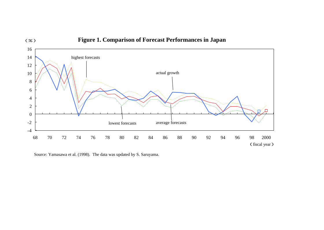
Figure 1. Comparison of Forecast Performances in Japan

-4

-2

0

2

4

6

8

10

12

14

16

68 70 72 74 76 78 80 82 84 86 88 90 92 94 96 98 2000

actual growthrates

highest forecasts

lowest forecasts

（fiscal year）

（％）

Source: Yamasawa et al. (1998). The data was updated by S. Saruyama.

average forecasts

Figure 2-A. A Comparison of Type 1 Index and the EPA-CI (1995=100)

60

80

100

120

140

1980:1 1982:1 1984:1 1986:1 1988:1 1990:1 1992:1 1994:1 1996:1 1998:195

100

105EPA-CI（left）

our indexwith smoother

(right)

shaded areas are thecontraction periods

our indexwithoutsmoother(right)

Figure 2-B. A Comparison of Type 2 Index and the EPA-CI (1995=100)

60

80

100

120

140

1980:1 1982:1 1984:1 1986:1 1988:1 1990:1 1992:1 1994:1 1996:1 1998:185

90

95

100

105

110EPA-CI（left）

our indexwith smoother

(right)

shaded areas are thecontraction periods

our indexwithoutsmoother(right)